


Abstract
The joint time–frequency (TF) distribution is a critical method of describing the instantaneous frequency that changes with time. To eliminate the errors caused by strong modulation and noise interference in the process of time-varying fault feature extraction, this paper proposes a novel approach called second-order time–frequency sparse representation (SOTFSR), which is based on convex optimization in the domain of second-order short-time Fourier transform (SOSTFT) where the TF feature manifests itself as a relative sparsity. According to the second-order local estimation of the phase function, SOSTFT can provide a sparse TF coefficient in the short-time Fourier transform (STFT) domain. To obtain the optimal TF coefficient matrix from noisy observations, it is innovatively formulated as a typical convex optimization problem. Subsequently, a multivariate generalized minimax concave penalty is employed to maintain the convexity of the least-squares cost function to be minimized. The aim of the proposed SOTFSR is to obtain the optimal STFT coefficient in the TF domain for extraction of time-varying features and for perfect signal reconstruction. To verify the superiority of the proposed method, we collect the multi-component simulation signals and the signals under variable speed from a rolling bearing with an inner ring fault. The experimental results show that the proposed method can effectively extract the time-varying fault characteristics.
Export citation and abstract BibTeX RIS
1. Introduction
As a traditional method of processing signals, spectrum analysis can diagnose and locate machine faults with the help of the characteristic frequency [1, 2]. It has been widely used in fault identification of rolling bearings [3, 4]. However, traditional spectrum analysis only applies to the stable working condition with fixed speed. The rotation frequency and fault characteristic frequency (FCF) of each component will often change with rotation speed in engineering practice. Therefore, traditional spectrum analysis fails to solve this problem [5]. For accurate fault identification and early warning, it is necessary to eliminate the influence of speed and load change. Time–frequency analysis (TFA) has close ties with the tendency for the frequency characteristics of a signal to change with time. Thus, TFA can be used as a powerful tool to analyze time-varying fault characteristics under non-stationary working conditions [6, 7].
Presently, there are advantages and disadvantages to the commonly used TFA methods. Traditional TFA technology has various defects, such as the Heisenberg uncertainty principle, cross terms and mode aliasing [8–10]. These defects seriously interfere with representations of the signal features, leading to difficulty in determining the time-varying rule. Thetwo typical methods are short-time Fourier transform (STFT) and empirical mode decomposition (EMD) [11, 12]. In theory, STFT is based on the inner product and on the idea of fixing sliding windows. Therefore, the choice of window function and window width has an influence on the correctness of the analysis results. EMD belongs to the algorithm of signal adaptive decomposition. Nevertheless, EMD and its upgraded versions such as ensemble EMD still have some problems, such as a lack of theoretical basis and mode aliasing [13]. Subsequently, variational mode decomposition and empirical wavelet transform have been successively proposed to achieve multi-component signal decomposition [14, 15]. However, parameter selection is still inevitable. Daubechie et al proposed the synchrosqueezed wavelet transform (SWT) [16], which plays an important role in improving the energy concentration of the time–frequency (TF) plane both theoretically and practically. In this method, the complex spectrum of wavelet transform is squeezed and rearranged along the frequency axis to obtain a more concentrated TF representation. SWT has expanded into the field of multivariable signal processing [17]. However, this method is poor in noise immunity and requires an accurate estimation of the instantaneous frequency (IF). Recently, based on the theoretical framework of the synchrosqueezing transform (SST), several TFA methods, such as STFT-based SST (FSST), second-order STFT-based SST (FSST2), four-order STFT-based SST (FSST4) [18], synchroextracting transform (SET) [19], synchroextracting chirplet transform [20] and high-order SST [21], have been put forward to address these problems. These synchrosqueezing-based methods are all post-processing processors and do not change the qualitative behavior of the TF representation. Objectively, the actual analysis result of this kind of method still depends on standard STFT or wavelet transform (WT). Based on the above descriptions, optimal STFT plays a significance role in time-varying feature identification from the TF plane, especially under the circumstances of outliers and strong interference. To address this common problem, this paper introduces high-order STFT which is based on the high-order derivative of amplitude and phase of the signal [22]. In particular, considering the calculation cost and the feasibility of practical application, we derive a second-order short-time Fourier transform (SOSTFT) to obtain a sparse TF coefficient, which is based on second-order local estimation of the phase function.
In contrast with the commonly used post-processing method, this paper focuses on obtaining the optimal STFT coefficients. The commonly improved STFT methods include adaptive STFT [11, 23] and multi-resolution STFT [24]. Usually, these methods work well under certain assumptions. Nevertheless, significant reconstruction errors will appear if these methods are used to deal with signals with strong amplitude modulation and frequency modulation (AM–FM). In particular, the signals collected from industrial equipment often contain noise and are in non-stationary working conditions, which often leads to unsatisfactory results. Recently, Zhu has proposed two sound methods to reconstruct multi-component signals [25]. The methods are aimed at eliminating the influence of strong noise and outliers with a better loss function. However, it cannot precisely reconstruct strong modulation signals under the condition of loud noise.
Inspired by the idea that the TF transformation coefficient is the local maximum of the signal energy in the TF plane, we can innovatively transform the problem of time-varying feature extraction into a typical convex optimization problem. In other words, our goal is to get a sparse approximate representation in the TF plane. Convex optimization, a subfield of mathematical optimization, studies the problem of minimizing convex functions defined in convex sets. Due to the sound properties of convex optimization, we can obtain the approximate solution for many non-convex optimization problems in our daily life [26, 27]. This paper proposes a robust approach called second-order time–frequency sparse representation (SOTFSR), which defines SOSTFT as the matrix operator and the optimal TF coefficients as an objective function of the convex optimization problem, in contrast to extant TFA methods like SST. Based on the Huber function and minimax concave (MC) penalty, this paper introduces a multivariate generalized minimax concave (GMC) penalty to guarantee the strict convexity of the regularized linear least-squares cost function [28–30]. Therefore, the obtainment of STFT coefficients of interest through our proposed SOTFSR method is critical for subsequent feature extraction and mode reconstruction.
The rest of this paper is arranged as follows: in section 2, we will give a theoretical introduction to SOSTFT and SOTFSR. In section 3, numerical analyses of simulation signals with multi-components will be presented to verify the feasibility of the proposed method in dealing with strong frequency modulation signals. In addition, the results provided by STFT, SST and SET will be used for comparison. In section 4, we will analyze gravitational wave signals and vibration signals of mechanical equipment with inner faults under variable speed, which will further demonstrate the feasibility of the proposed method. Our conclusions will be given in section 5.
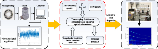
Figure 1. Flowchart of the proposed method. Download figure:
2. Theory description
2.1. Second-order short-time Fourier transform
The equation of a multi-component AM–FM signal is defined as follows:
where  is a positive integer representing the number of AM–FM components,
  and
and  are the instantaneous amplitude and instantaneous phase function of the
  component, respectively, and
  is determined as the IF. If we set
  as a real window function in the Schwartz class, the STFT of signal
  is expressed as:
The first-order approximation STFT of signal  can be written as follows:
where  is the Fourier transform of window function
  . From equation (3), the original signal
  can be easily obtained as:
The modified STFT of f(t) in equation (2) can be rewritten as:
Using the Taylor series approximation, the complex-valued function  can be estimated as:
where ![${\rho _n}\left( t \right) = {\left. {\frac{{{d^n}}}{{d{\mu ^n}}}\left[ {\frac{{f\left( {t + \mu } \right){e^{ - j\phi ^{\prime}(t)\mu }}}}{{f\left( t \right)}}} \right]} \right|_{\mu = 0}}$](https://content.cld.iop.org/journals/0957-0233/32/2/025116/revision3/mstabb50fieqn13.gif) . Substituting equation (6) into (5), we can obtain the high-order form of STFT. Details are as follows:
. Substituting equation (6) into (5), we can obtain the high-order form of STFT. Details are as follows:
where  denotes the nth-order derivative of
  and
and  . Equation (7) can obtain the Nth-order approximation of STFT and be expressed as follows:

where  is a feature analysis matrix and
  is an original signal matrix.
In further detail,  and
and  are respectively calculated as:

Then, the nth-order derivative of  can be estimated as:
Combining (8) and (11), and setting  ,
,  can be approximately calculated as:
For simplicity, equation (12) can be expressed as a matrix product:

From equation (13), the original signal can be reconstructed by the equation ![$f\,(t) \approx \left[ {\bar G_N^{ - 1}(1,1),\ldots,\bar G_N^{ - 1}(1,N + 1)} \right]{S_N}(t)$](https://content.cld.iop.org/journals/0957-0233/32/2/025116/revision3/mstabb50fieqn24.gif) .
.
Concretely speaking, when  , the second-order approximation of STFT for
  , i.e. SOSTFT, can be obtained from equation (8). It is derived to strike a balance between reducing computing costs and maintaining good TF analysis performance.
2.2. Second-order time–frequency sparse representation
Many signal-processing techniques can be regarded as a problem of the sparse approximation solution in the TF domain. Usually, the convex optimization scheme can be used to seek a sparse approximate solution to a system of linear equations. In this section, the SOTFSR method proposed herein introduces a novel non-convex penalty for sparse-regularized linear least squares, in order to strictly keep the minimized convexity of the least-squares cost function.
There is no doubt that standard STFT is an important theoretical basis for TFA. The STFT values of the analyzed signal are given at the sample points regarded as the approximate points of the time-varying fault features. Thus, the proposed SOTFSR can be promoted in the TF sparsity and transformed to solve the following cost function based on convex optimization:
where  is an actual measured vibration signal and
  is the STFT coefficients. In terms of the sparse transformation, the matrix
  represents the inverse SOSTFT operator defined in equation (8) and
  . The non-convex penalty
  is a sparsity-promoting penalty function, which is parameterized by a matrix B. The convexity of
  largely depends on B. It also should be pointed out that the choice of B will depend on A. l1 norm is a common penalty to introduce sparse representations, but it may produce local suboptimal solutions. This paper introduces a multivariate GMC penalty, which is based on the generalized Huber function [28–30].
Firstly, the Huber function  is defined as:
The MC penalty function is defined as:
Accordingly, the MC penalty can be expressed as:

The above equation for the MC penalty will be used to generalize the GMC penalty. Then, we will define scaled versions of the Huber function and MC penalty, respectively. The scaled Huber function is defined as:
Similar to equation (17), the scaled MC penalty function is defined as:

Letting  , we define the generalized Huber function as:
Subsequently, we introduce a multivariate generalization of the MC penalty (17), which is generated by using the l1 norm and the generalized Huber function defined in equation (20). The GMC penalty function is defined as:

where  corresponds to the generalized Huber function. Matrix B is used to accurately describe the convexity of G(c), and its selection is related to matrix A, namely
  .
.
Given the inverse SOSTFT coefficient matrix A, we can simply set:

 (22) where the parameter
  controls the convexity of the penalty
  . When
  , the penalty
  becomes the typical l1 norm. According to our experiment, better results can be obtained if the value of
  ranges from 0.5 to 0.8.
The minimum value of equation (14) can be solved by the forward/backward algorithm, which can be rewritten as a saddle point problem as shown below:

where  is the saddle function and the matrix
  is the optimal STFT coefficients by the proposed SOTFSR method. In addition,
  represents the auxiliary variable. When the local optimum value of equation (23) is obtained, the one-dimensional signal component of interest x can be obtained by
  .
.
Based on this, assuming that the number of modes K is known, we can achieve accurate estimation of the fault characteristic component in the method described in [31]. This technique heavily relies on the minimization of the following energy function:
where  is the estimation of different modes with time-varying fault characteristics.
  is one of the TF representations given by
  , which is provided in equation (23).
  and
and  are regularization parameters which can maximize the balance between smoothness of
  and energy. In general, the values of
  and
and  have little effect on the final analysis results.
3. Numerical simulation analysis
To verify the validity of the proposed method, numerical simulation analysis is firstly applied to multi-component signals. The ultimate goal is to accurately extract time-varying features and to reconstruct signals. The proposed method based on the convex optimization is employed to deal with noise signals. The analog simulation signal is expressed in the following form:


where  is a typical multi-component AM–FM signal. The IF corresponding to
  and
and  can be expressed as
  and
and  . To test noise immunity, Gaussian white noise is added to the signal
  and the signal-to-noise ratio (SNR) is calculated as 3 dB.
The time- and frequency-domain waveforms of multi-component signals are respectively plotted in figure 2. Judging from this, traditional signal-processing methods, like fast Fourier transform (FFT), cannot effectively reflect the rule that frequency changes with time. Meanwhile, noise will interfere with identification of multi-component signals. The ideal time-varying feature relevant to multi-component signals is shown in figure 3. The red and blue TF curves respectively correspond to IF1 and IF2. It clearly shows the law of a mode with sinusoidal phase and a linear chirp. Subsequently, figure 4 shows TF analysis results obtained by four different methods, including STFT, SST and SET. Due to the influence of noise, the results provided by STFT are ambiguous in the TF plane in figure 4(a). SST and SET are typical TF rearrangement algorithms based on IF estimation. The calculation results are shown in figures 4(b) and (c). The results show that SST has low energy aggregation and SET shows a dramatic improvement in performance. However, irrelevant signal components still exist in figure 4(c). Compared with SST and SET, the proposed SOTFSR has clear advantages in sharpening TF representations in figure 4(d).

Figure 2. Time and frequency domain waveform of simulated signal.
Download figure:
Standard image High-resolution image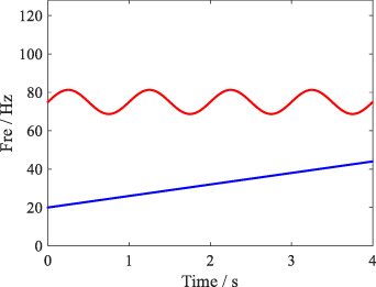
Figure 3. Ideal time–frequency curve of simulated signal.
Download figure:
Standard image High-resolution image
Figure 4. TF analysis results provided by four different methods.
Download figure:
Standard image High-resolution imageRenyi entropy is a means of quantitative evaluation of information uncertainty. The more random the signal is, the bigger the uncertainty and the corresponding entropy are, and vice versa. In the field of TF analysis, more concentrated TF energy means that the uncertainty is less and the Renyi entropy value is smaller. To quantitatively evaluate the effectiveness of TFA, we choose Renyi entropy as an assessment criterion [19]. The results obtained in different TF methods are listed in table 1. The proposed method clearly has a smaller Renyi entropy, which indicates that this method is better in TF energy aggregation.
Table 1. Comparison of Renyi entropy between different TF methods.
| Methods | STFT | SST | SET | Proposed SOTFSR |
|---|---|---|---|---|
| Renyi entropy | 18.08 | 14.09 | 12.24 | 11.06 |
To demonstrate the robustness to noise of the proposed method, we provide the SNR obtained by the three methods in different SNR simulation signals. Figure 5 represents the SNR changing curves obtained in these three methods. The vertical coordinate denotes the SNR after signal reconstruction. A larger SNR value in the vertical coordinate of figure 5 means a better performance in feature extraction. From the comparison shown in figure 5, we can conclude that the proposed method is superior in signal reconstruction.
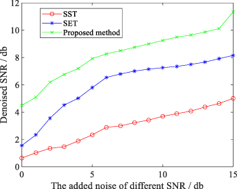
Figure 5. Comparison of reconstruction performance in different SNRs.
Download figure:
Standard image High-resolution image4. Experimental data analysis
5. Case 1: application to gravitational wave signal
Gravitational waves are one of the most important predictions of general relativity [32]. After nearly a century of efforts, GW150914 was the first gravitational wave signalsuccessfully detected on September 14th 2015. The received signal proves that the prediction of general relativity is right. There are two black hole systems in the universe which may be combined into a larger one. We will use the method proposed in this paper to analyze gravitational wave signals. It is aimed at recognizing the law that gravitational wave intensity changes with time and frequency, which is observed by a Laser Interferometer Gravitational-Wave Observatory detector.
The observed initial Hanford signal has a length of 4096 samples and the corresponding time-domain waveform is shown in figure 6(a). Then, the TFA by means of STFT is plotted in figure 6(b). It is observed that the TF blur seriously affects the resolution of feature recognition. Then, gravitational wave signals are analyzed by an advanced method FSST2, and by the proposed method. The main reason for choosing FSST2 as the comparison method is that its computational complexity is acceptable. The analysis results are shown in figure 7. Clearly, the result provided by the proposed SOTFSR in figure 7(b) has fewer cross-interference phenomena and clearer TF representations.
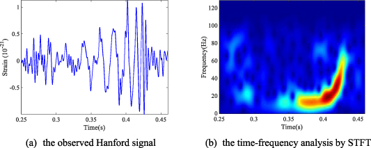
Figure 6. Original TF representations of gravitational waves.
Download figure:
Standard image High-resolution image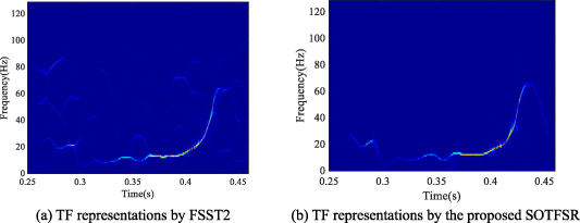
Figure 7. TF representations provided by FSST2 and the proposed SOTFSR.
Download figure:
Standard image High-resolution imageThen, the time-varying feature extraction is applied to figure 7 and the corresponding result is shown in figure 8. Theoretically, FSST4 can obtain more accurate estimations of the instantaneous frequencies of the modes making up the signal by using higher-order approximations for both the amplitude and phase. However, FSST4 will make calculation more complex, influencing its practical application in engineering. The TF representations generated by FSST4 are shown in figure 9. In the field of TF analysis, smaller Renyi entropy indicates the concentrated TF representation is better [19]. Through calculation, the Renyi entropy corresponding to figures 8 and 9 is 13.2889, 11.1412 and 12.0375, which demonstrates that the proposed method has satisfactory performance. We believe that the proposed method can detect the changing feature more effectively. The extracted feature is highlighted in green and manganese purple in the TF plane. Based on the time-varying feature extraction, the mode reconstruction is achieved. For the purpose of evaluation, we consider the difference between the reconstructed signal and the numerical relativity waveform obtained through independent calculation based on [32]. On the basis of the Baumgarte–Shapiro–Shibata–Nakamura formulation of Einstein's equations, Campanelli presents a new algorithm for obtaining the numerical relativity waveform [33]. Thus, numerical relativity waveforms can be considered as theoretical true values. The reconstruction error of the two TF methods is expressed in figure 10. It is certain that the proposed SOTFSR in this paper has a smaller reconstruction error and better performance.
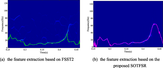
Figure 8. Performance comparison between FSST2 and SOTFSR.
Download figure:
Standard image High-resolution image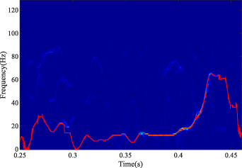
Figure 9. Feature extraction provided by FSST4 in the TF plane.
Download figure:
Standard image High-resolution image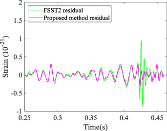
Figure 10. Reconstruction error by different TF methods.
Download figure:
Standard image High-resolution image6. Case 2: application to mechanical equipment failure signal
To verify the feasibility of the approach, this study conducts vibration signal analysis under time-varying rotational speed [34, 35]. This is aimed at achieving high-resolution representation of fault characteristic components in the TF plane under variable conditions. The data are collected by an ICP accelerometer placed on the faulty bearing of a SpectraQuest machinery fault simulator (MFS-PK5M) and the specific experimental equipment is shown in figure 11. A motor is used to drive the shaft and the rotational speed is adjusted by an AC drive. Two ER16 K ball bearings are located at the end of the shaft. It should be pointed out that the left bearing is in good condition while the right one requires replacement, i.e. is faulty. Table 2 clearly shows the structure parameters of the rolling bearings under study. The fault characteristic coefficient (FCC) corresponding to the outer race fault (FCCo) and the inner race fault (FCCI) can be calculated as follows [36].
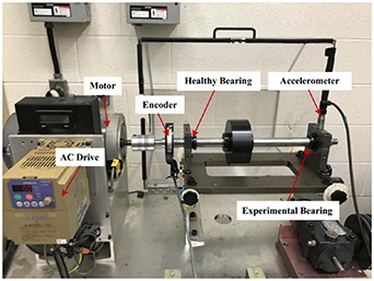
Figure 11. Experimental equipment.
Download figure:
Standard image High-resolution imageTable 2. Parameters of bearings.
| Bearing type | Pitch diameter | Ball diameter | Number of balls | FCCI | FCCO |
|---|---|---|---|---|---|
| ER16K | 38.52 mm | 7.94 mm | 9 | 5.43 | 3.57 |
where nb
is the number of rolling elements, d is the diameter of the rolling element, D is the pitch diameter of the bearing, and  is the angle of the load from the radial plane. It is clear that FCC (FCCo or FCCI) is the ratio of the FCF to the shaft rotational frequency (SRF). Under time-varying speed conditions, the FCC can be used to identify the failure mode because it is determined by the bearing structural parameters and also immune to velocity variation. By identifying the instantaneous fault characteristic frequency (IFCF) and the instantaneous shaft rotational frequency (ISRF) from the extracted TF curves, the average curve-to-curve ratio can be determined by theoretical calculation. By comparing the actual calculated curve-to-curve ratio with the FCC determined by the bearing structural parameters, the bearing faults can be diagnosed under the condition of time-varying speed without using a tachometer to measure the rotational speed.
Moreover, an encoder, which is regarded as a tool for comparative analysis, is employed to measure the shaft rotational speed. The sampling frequency of the analyzed signals is set as 200 kHz at 10 s intervals. Down-sampling must be performed because the high sampling rate results in high data volume. In order to verify that this method is effective in many areas, we collect the vibration signals from a faulty bearing with an inner race defect and decrease the rotational speed from 25.1 to 13.1 Hz.
The down-sampled bearing vibration signal is shown in figure 12. From the calculation results of FFT operation plotted in figure 12(b), we cannot inspect the FCF component. Envelope spectrum analysis is a common method of vibration signal analysis of mechanical equipment and the corresponding results are shown in figure 13. Unfortunately, we still cannot effectively identify the fault characteristics, either from the time-domain waveform or spectrum analysis results.
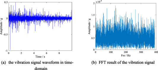
Figure 12. Down-sampled bearing signal shown in time and frequency domains.
Download figure:
Standard image High-resolution image
Figure 13. Envelope spectrum of the down-sampled bearing vibration signal.
Download figure:
Standard image High-resolution imageThe results provided by the envelope spectrum of the signal after 1 k high-pass filter are plotted in figure 14. The FCF, its harmonics, and the SRF cannot be identified in the spectrum analysis results. Generally, bearing faults can be diagnosed through identifying the FCF in the frequency spectrum of the vibration signals. However, under the time-varying rotational speed, the fault characteristics of bearings are often non-stationary. Therefore, traditional spectral analysis methods based on Fourier transform will be ineffective.
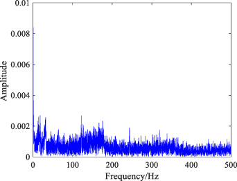
Figure 14. Frequency spectrum provided by high-pass filter and envelope analysis.
Download figure:
Standard image High-resolution imageParametric TFA is an important technical means of realizing fault diagnosis of mechanical equipment under variable working conditions. To date, the traditional TF method STFT and its advanced version, second-order STFT-based SST (FSST2), still plays an important role in TF representations of multi-component signals in noisy environments. At the same time, STFT and FSST2 are chosen as analysis tools of comparison, so as to reduce calculation. The results generated by STFT and FSST2 are shown in figure 15.
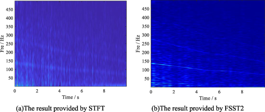
Figure 15. TF analysis results provided by STFT and FSST2.
Download figure:
Standard image High-resolution imageDue to the defects of the theory, a blur of TF occurs in the method of STFT, with a high level of noise in the TF plane displayed in figure 15(a). Therefore, it is necessary to improve the TF resolution of STFT. According to figure 15(b), in contrast to STFT, FSST2, which is based on the SST framework, is better at dealing with non-stationary vibration signals. However, the time-varying feature corresponding to the FCC is indistinct and the low-frequency speed signal is not recognized. In other words, the performance of FSST2 still cannot meet the analysis requirements in sharpening TF representation. Next, we adopt a new method, SOTFSR, which uses the second-order STFT framework and convex optimization scheme, with the results plotted in figure 16. Fortunately, FCCs and rotational speed signals are successfully extracted by the proposed method. Compared with figures 15 and 16, we can conclude that the proposed approach is better at fault feature extraction of complex multicomponent vibration signals.
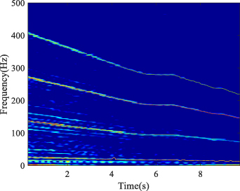
Figure 16. Results provided by the proposed SOTFSR.
Download figure:
Standard image High-resolution imageThe number of feature curves that require extracting is set as 4. Subsequently, figure 17 shows the extraction of time-varying feature curves by the proposed SOTFSR. Through the extracted time-varying features, it is estimated that the bottom TF curve and the second-lowest TF curve respectively stand for ISRF and IFCF. By theoretical calculation, the average curve-to-curve ratio is determined as 5.47, which matches the FCCI. The two highest curves in figure 17 are related to the FCFs twice and three times (2FCCI and 3FCCI). For clarity, figure 18(a) demonstrates the estimated ISRF and the identified IFCF. Moreover, the shaft encoder signal can provide the measured ISRF. Figure 18(b) shows a comparison between the estimated ISRF and the measured ISRF. The average error, |estimated ISRF–measured ISRF|/measured ISRF, is close to 2.41%. Thus, based on the proposed method of SOTFSR, the conclusion can be drawn that the identified failure mode belongs to the inner ring fault, which is consistent with the actual situation. Additionally, the estimated ISRF is so accurate that we can analyze orders without a tachometer in future work.

Figure 17. Extracted curves from the TFR by SOTFSR.
Download figure:
Standard image High-resolution image
Figure 18. Extracted time-varying features corresponding to ISRF and IFCF.
Download figure:
Standard image High-resolution image
7. Conclusions
Time-varying fault feature extraction is an important technique of TF analysis and signal reconstruction. However, its performance relies on signal modulation and noise interference. To resolve these problems, we use GMC penalty functions with the help of a convex optimization to promote the TF sparsity of the coefficients in the SOSTFT domain. The main contents of this paper are summarized as follows: (1) we introduce a SOSTFT which is based on second-order local estimation of the phase function. The aim of SOSTFT is to obtain a high-resolution TF representation and set a TF transform operator in the following convex optimization scheme; (2) subsequently, the work of time-varying feature extraction can be innovatively transformed to a typical convex optimization problem. GMC penalty is introduced to maintain the convexity of the objective function so as to obtain the STFT coefficient of interest in the TF domain. On this basis, accurate time-varying feature identification can be accomplished by the proposed method of SOTFSR; (3) to verify the feasibility of this approach, we carry out the numerical simulation of multi-component signals from a faulty bearing under variable speed. It is worth mentioning that the extracted feature corresponding to ISRF can be used for order-tracking analysis in the process of dealing with practical engineering signals. Consequently, the result proves that the proposed SOTFSR has clear superiority in dealing with vibration signals of mechanical equipment.
Acknowledgments
This work was supported by the National Natural Science Foundation of China under Grant No. 51805382.
Competing Interests
The authors declare that there are no conflict of interests regarding the publication of this article.