Article

Assessment of DUACS Sentinel-3A Altimetry Data in the Coastal Band of the European Seas: Comparison with Tide Gauge Measurements

by
Antonio Sánchez-Román
1,*,
Ananda Pascual
1,
Marie-Isabelle Pujol
2,
Guillaume Taburet
2,
Marta Marcos
1,3 and
Yannice Faugère
2
1
Instituto Mediterráneo de Estudios Avanzados, C/Miquel Marquès, 21, 07190 Esporles, Spain
2
Collecte Localisation Satellites, Parc Technologique du Canal, 8-10 rue Hermès, 31520 Ramonville-Saint-Agne, France
3
Departament de Física, Universitat de les Illes Balears, Cra. de Valldemossa, km 7.5, 07122 Palma, Spain
*
Author to whom correspondence should be addressed.
Remote Sens. 2020, 12(23), 3970; https://doi.org/10.3390/rs12233970
Submission received: 26 October 2020 / Revised: 23 November 2020 / Accepted: 1 December 2020 / Published: 4 December 2020
(This article belongs to the Special Issue Calibration and Validation of Satellite Altimetry)

Abstract

:
The quality of the Data Unification and Altimeter Combination System (DUACS) Sentinel-3A altimeter data in the coastal area of the European seas is investigated through a comparison with in situ tide gauge measurements. The comparison was also conducted using altimetry data from Jason-3 for inter-comparison purposes. We found that Sentinel-3A improved the root mean square differences (RMSD) by 13% with respect to the Jason-3 mission. In addition, the variance in the differences between the two datasets was reduced by 25%. To explain the improved capture of Sea Level Anomaly by Sentinel-3A in the coastal band, the impact of the measurement noise on the synthetic aperture radar altimeter, the distance to the coast, and Long Wave Error correction applied on altimetry data were checked. The results confirmed that the synthetic aperture radar altimeter instrument onboard the Sentinel-3A mission better solves the signal in the coastal band. Moreover, the Long Wave Error processing contributes to reduce the errors in altimetry, enhancing the consistency between the altimeter and in situ datasets.

Graphical Abstract

1. Introduction

Since 1992, altimeter missions have been providing accurate measurements of sea surface height (SSH) [1]. However, there is still a degree of uncertainty in altimeter measurements and in the geophysical corrections applied in the SSH computation [2,3,4,5]. Traditional altimetry retrievals have often been unable to produce meaningful signals of sea level change in the coastal zone due to the typically shallower water, bathymetric gradients, and shoreline shapes, among other things [6].
In the recent past, a lively international community of scientists has been involved in the research and development of techniques for coastal altimetry, with substantial support from space agencies such as the European Space Agency (ESA), the Centre National d’Études Spatiales (CNES), and other research institutions [7]. Efforts have aimed at extending the capabilities of current altimeters closer to the coastal zone. This includes the application of improved geophysical corrections, data recovery strategies near the coast using new editing criteria, and high-frequency along-track sampling associated with updated quality control procedures [6,7,8,9]. Concerning the geophysical corrections, one of the major improvements is in the tide models where the tidal component is not part of the observed signal [10] and needs to be removed [7].
In parallel with these efforts, the Sentinel-3A satellite was launched in February 2016 as part of the European Union Copernicus Programme. It became fully operational in July 2016. The Sentinel-3 mission is jointly operated by the ESA and the European Organisation for the Exploitation of Meteorological Satellites (EUMETSAT) to deliver, among other things, operational ocean observation services [11]. The Sentinel-3A onboard altimeter, a synthetic aperture radar altimeter (SRAL), is based on a principle proposed by [12]: the synthetic aperture radar mode (SARM). The SRAL has two advantages over the conventional altimeter: (i) a finer spatial resolution in the along-track dimension [13] and (ii) the higher signal-to-noise ratio of the received signal and lower speckle noise from SAR waveforms [14,15], providing enhanced Sea Level Anomaly (SLA) measurements in the coastal zone [15].
The Sentinel-3A data are processed by EUMETSAT (https://www.eumetsat.int), which freely distributes level 1 and level 2 products. These products are in a second step reprocessed through the Data Unification and Altimeter Combination System (DUACS) altimeter multi-mission processing system (https://duacs.cls.fr). The DUACS system provides directly usable, high-quality near-real-time and delayed time (DT) global and regional altimeter products [1,5]. The main processing steps include product homogenisation, data editing, orbit error correction, reduction in Long Wavelength Errors (LWE), and the production of along-track and mapped sea level anomalies. The DUACS processing [3] is based on the altimeter standards given by L2P (Level-2 Plus) products (see e.g., [16]). They include the most recent standards recommended for altimeter global products by agencies and expert groups such as the Ocean Surface Topography Science Team (OSTST) and the ESA Quality Working groups.
More than 25 years of level-3 (L3) and level-4 (L4) altimetry products were reprocessed and recently delivered as the DUACS DT 2018 version [5]. L3 products for repetitive altimeter missions are based on the use of a mean profile [3,17] that allows collocating the SSH of the repetitive tracks and retrieving a precise mean reference to compute SLAs [5]. SLAs are often used instead of absolute dynamic topography, defined as the differences between SSH and the geoid height, because the geoid is not perfectly known at scales smaller than 150 km from space gravity missions [17]. To solve this, a mean sea surface model based on altimetry data that contains the sum of the geoid height and the mean dynamic topography is used [17].
The along-track SLA products are affected by the uncertainties in the geoid surface model and also by (i) instrumental errors, (ii) environmental and sea state errors, and (iii) the precision of geophysical corrections. These elements introduce errors in the measurements [18]. To minimise their impact, DUACS-DT2018 re-processing considers the most up-to-date altimetry corrections, such as (a) dry and wet troposphere corrections, (b) ionospheric correction, (c) sea state bias correction, (d) dynamic atmospheric correction (DAC), and (e) the ocean tide. Some of these instrumental and environmental errors remain in the along-track products delivered to final users, mainly due to the imprecision of the corrections applied.
Altimeter data are widely calibrated and validated by comparison with in situ timeseries [19]. Tide gauge measurements are commonly used. In situ and altimetric observations are complementary and are often assumed to observe the same signals (e.g., [20]). The comparisons with in situ observations allow us to obtain altimetry errors relative to the external measurements and provide an improved picture of SSH. The paper [5] assessed gridded products in coastal areas through a comparison with monthly tide gauge measurements from the Permanent Service for Mean Sea Level (PSMSL) Network [21]. The procedure described in [19,22] was used. The paper [5] reported a global reduction of 0.6% in variance when using the DUACS-DT2018 data with respect to the previous DUACS-DT2014 dataset [3], with a clear improvement along the Indian coast, Oceania, and Northern Europe.
The consistency between altimeter gridded products and tide gauge data in the coastal region was also investigated at global [23,24] and regional (Mediterranean basin) scales [25,
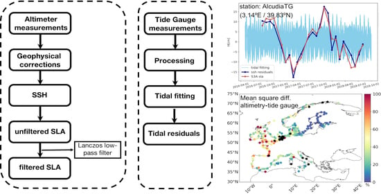
26]. Mean square differences between tide gauge and gridded altimetry (see Section 3.1 in the text) ranging between 30% and 90% were obtained by [23] in the European coasts, whilst these differences were reduced to around 40% [24] thanks to improved geophysical corrections (i.e., a new DAC) applied to altimetry data with root mean square differences (RMSD) between gridded altimetry and tide gauges of 4.43 cm in the Atlantic Ocean. The paper [25] found a median value for the correlation altimetry—a tide gauge of 0.79 in the Mediterranean Sea.
These works used low-pass filtered (monthly averaged) tide gauge records from PSMSL and the Global Sea Level Observing System (GLOSS)/Climate Variability and Predictability (CLIVAR) [27] to remove high frequencies not resolved by the altimetry gridded products used for inter-comparisons. Thus, a comparison at higher frequencies between a specific regional product for the whole European coast and a high-density tide gauge dataset is, to our knowledge, still lacking.
Here, we present an assessment of the Copernicus Marine Environment Monitoring Service (CMEMS)/DUACS along-track (L3) altimeter regional operational products in the European seas using in situ tide gauges from the Copernicus Marine Environment Monitoring Service (CMEMS) catalogue. The aim is to validate the Sentinel-3A SAR mode SLAs against the equivalent in situ tide gauge measurements. Six-hour time series of tide gauge measurements will be compared with the 1 Hz along-track altimetry data from the Sentinel-3A satellite mission, this strongly enhancing both the spatial and temporal resolution of the results reported by [5]. We expect to obtain a more detailed assessment of DUACS-DT2018 products in the European seas at the both regional and sub-regional level. This inter-comparison has been also conducted by using SLA from the Jason-3 satellite mission to investigate the improvements of the Sentinel-3A mission over the latter in the coastal band.

2. Materials and Methods

2.1. Sea Level Anomalies from Altimetry

The DUACS-DT2018 along-track (L3) regional altimetry products for the European seas were released by CMEMS in 2018. We use delayed-time (quality controlled) reprocessed altimeter along-track SLA products computed with respect to a twenty-year (1993–2012) mean for the satellite missions Jason-3 and Sentinel-3A. These products have a spatial sampling of around 7 km, corresponding to the upstream 1 Hz products sampling. Filtered and unfiltered SLA measurements are provided. In this work, we have used both. Unfiltered SLA is the raw SLA (i.e., not filtered) measured by the instrument. Unless otherwise stated, SLA will refer to unfiltered SLA throughout the text, except for Section 3.3, where we specifically compare the results obtained from both SLAs.
Filtered SLA is computed for regional Europe products in the DUACS procedure by applying a Lanczos low-pass filter with a cut-off wavelength of around 40 km to SLA measurements (e.g., [13]). The aim is to remove the noise signal and the short wavelengths affected by the noise [18]. This procedure is discussed in [3]. This low-pass cut-off length is the minimal one that can be applied to along-track SLA to reduce noise effects and preserve as much as possible the physical signal. Filtered SLA is not sub-sampled to keep the 1 Hz full resolution. We decided to focus on the reference low-rate (1 Hz) SLAs instead of high-rate (i.e., 20 Hz) SLAs, because the former are produced by DUACS and delivered by CMEMS to the entire oceanographic community. The high-frequency 20 Hz products are not available for most users. Figure 1 shows a flowchart explaining the DUACS procedure applied to the altimetry data.
The time period analysed spans from May 2016 to September 2018. The areas investigated are the whole European coast, the Baltic Sea, the Arctic Sea, North-West Shelves (NWS) region, the Iberian-Biscay-Irish (IBI) region, and the central-western Mediterranean Sea (Figure 2).

2.2. Tide Gauge Observations

The sea-level records used to compare with satellite altimetry were obtained from the CMEMS In Situ Thematic Assembly Centre (TAC) data repository. The Copernicus catalogue provides data of 485 tide gauge stations along the World Ocean coasts, which are updated within a few weeks or a few months. This dataset covers the time period spanning from January 2010 to the present. Six-hourly tide gauge records were used according to the following procedure (Figure 1): the 445 tide gauge stations located in the European seas’ domain were initially considered for this study. The quality flags of the tide gauge records were checked and observations with anomalous SSH data (values larger than three times the standard deviation of the time series) or changes in the vertical reference of the tide gauge were rejected. Additionally, tide gauge time series exhibiting a large variance (more than 20 cm2) with respect to altimetry data were removed, as they are considered not representative of ocean sea level changes and are likely related to local features (e.g., river discharge). Only tide gauges with at least a 70% yearly data coverage were selected in order to allow the analysis of the seasonal signal.
The final set consists of 370 stations (Figure 2). The stations and their information are listed in Table A1. Before they can be compared with altimeter data, tide gauge measurements have to be processed [7,19] to remove oceanographic signals whose temporal periods are not resolved by altimetry, thus avoiding important aliasing errors [6]. First, tidal components were removed from the sea level records using the u-tide software [28]. The annual and semiannual frequencies, mainly driven by steric effect, are kept in the tidal residuals since they are included in the altimetry data.
For consistency with the satellite altimetry data, the atmospherically induced sea level caused by the action of atmospheric pressure and wind was removed from the tidal residuals [7,25,29]. This high-frequency oceanic signal is badly sampled by altimeter measurements. To solve this problem, a combination of high frequencies of a barotropic model forced by pressure and wind (MOG2D) and low frequencies of a classical Inverted Barometer model was applied [30]. We used the DAC available at the Archiving, Validation, and Interpretation of Satellite Oceanographic Data (AVISO) website. The DAC data are provided as 6 h sea level fields on a 1/4° × 1/4° regular grid covering the global oceans. For each tide gauge site, the nearest grid point was selected and used to remove the atmospherically induced sea level from observations, previously converted into 6-hourly records [25]. Finally, the 6-hourly tidal residuals were corrected for vertical movements associated with glacial isostatic adjustment (GIA). Indeed, many studies have demonstrated the need for tide gauges to be corrected for vertical crustal land motion when compared to altimeter data, since tide gauges measure the relative sea level with respect to the land where they are grounded [19]. We considered GIA as the only source of vertical land motions and removed its effects from the tidal residuals using the Peltier mantle viscosity model (VM2) [31,32].

2.3. Method for Comparing Altimeter and In Situ Tide Gauge Records

The comparison method of altimetry with tide gauges consisted of co-locating both datasets in time and space. It was based on a particular track point selected for each tide gauge location as follows: we computed the correlations between each tide gauge record (tidal residuals) and SLA time series corresponding to track points within a radius of 1 degree around the tide gauge site and choose the most correlated track point. A minimum length of time series of 10 months (corresponding to approximately 10 cycles of Sentinel-3A) was set up to allow statistical significance [14]. Statistical analyses were performed between both datasets using all available data pairs (altimetry-tide gauge) for a given region.
The co-located altimeter and tide gauge measurements were analysed in terms of the RMSD and variance of the time series. The RMSD metric is commonly used to examine along-track altimeter data quality [14]. In addition, the robustness of the results was investigated according to [33] using a bootstrap method [34], which allows us to estimate quantities related to a dataset by averaging estimates from multiple data samples. To do that, the dataset is iteratively resampled with replacement. A total of 103 iterations were used to ensure that meaningful statistics such as standard deviation could be calculated on the sample of estimated values, thus allowing us to assign measures of accuracy to sample estimates.

2.4. Ancillary Data

The Global, Self-consistent, Hierarchical, and High-resolution Geography database (GSHHG) was used to estimate the nearest distance to the coast of the altimetry track points used to compare with tide gauges. The aim was to investigate the degradation of the altimetric signal as we approach the coast. The shorelines in the GSHHG database are constructed entirely from hierarchically arranged closed polygons and are available in five geographical resolutions. The early processing and assembly of the shoreline data is described in [35]. We used the latest data files for version 2.3.7 presently available and released on 15 June 2017 with the original full data resolution.

3. Results

3.1. Comparison of Sentinel-3A and Tide Gauges along the European Coasts

This section presents the statistics of the comparisons performed between the Sentinel-3A altimetry data and the tide gauge observations from the CMEMS catalogue in the coastal region in terms of errors (RMSD) and the variance of the differences between both datasets. The analysis has been conducted for the entire European coast and the following sub-regions: the Mediterranean Sea, the IBI and NWS regions, and the Baltic Sea (Figure 2). SLA measurements without filtering (Figure 1) were used. The bootstrapping technique [34] was applied to gain an estimation of the standard errors of the differences between both datasets.
The mean value of the RMSD between the Sentinel-3A satellite altimetry and tide gauges is 6.97 cm. The mean distance between the location of the tide gauge and the location of the corresponding altimeter data with the highest correlation is 80 km with a standard deviation of 33 km. Data from 342 tide gauge stations were compared with the Sentinel-3A data. Thus, 28 stations were rejected from the computation according with the selection criteria described in the previous section. These stations are located in the NWS region, the Mediterranean Sea, and the Arctic Sea (Table A1).
The rejected tide gauge time series showing a variance much larger than that found in the corresponding altimetry time series (RMSD between both datasets larger than 20 cm) were further investigated. We checked the shape of their time series, together with the quality flag data related to SSH, tide gauge position, and recorded atmospheric pressure. The aim was to investigate the presence of outliers in the tide gauge time series due to poor quality control not captured by satellite altimetry responsible for such large discrepancies, which could be corrected by the data providers. A subset of twenty-four tide gauge stations (Table A2) showed abnormal values in variance due to poor quality control that induced substantial RMSD when compared to the Sentinel-3A and Jason-3 altimetry data. This represents 5% of the tide gauge dataset in the European coasts.
Figure 3 shows the consistency between the altimetry and tide gauge data computed as follows:
variance ( tide   gauge altimeter ) variance ( tide   gauge )   ×   100 ,
where the variance of the tide gauge is associated with the variance of the signal. Consistency is expressed here as the mean square differences between both datasets, computed as the variance of the differences (altimetry—tide gauge) in terms of percentage of the tide gauge variance. This approach has already been applied by [23,24] to compare the satellite altimetry and tide gauge measurements at a global scale.
Overall, mean square differences lower than 10% are observed in most of the Baltic Sea (Figure 3b). Larger mean square differences of around 25% are observed in the Gulf of Finland, whereas they reach values between 15% and 50% and even larger values when in connection region with the North Atlantic Ocean. The mean square differences are between 20% and 50% for stations located in the Mediterranean Sea and the NWS region (Figure 3a).
If we analyse the results in terms of the RMSD (figure not shown), minimum mean errors of 3.41 cm were obtained in the Mediterranean Sea, whilst they increased until 10.72 cm for the NWS region. These results can be explained by the larger spatio-temporal variability observed in the NWS region (SLA mean variance of 206 cm2) with respect to that found in the Mediterranean basin (SLA mean variance of 47 cm2). Non-tidal variance, which is also larger in the former [36], contributes to the larger RMSD obtained in the NWS region.
The largest errors, which reach 100%, are mainly found in the Atlantic shore of the IBI region. This could be due to the imprecisions of the corrections applied (i.e., ocean tide) to the altimeter data.

3.2. Improvements of Sentinel-3A over Jason-3 Satellite Mission

In this section, we conduct an equivalent analysis on Jason-3 data. The Jason-3 satellite mission has an orbit repeat cycle of 9.91 days, whilst Sentinel-3A presents a repeat cycle of 27 days. To make the inter-comparisons between both satellite missions with in situ tide gauge observations comparable, SLA from Jason-3 was sub-sampled to retain every third point along the tracks to emulate the Sentinel-3A cycle. The tide gauge stations (270 stations) common to both satellite missions were used. The results obtained for the whole European coasts are summarised in Table 1.
Notice that the rejected tide gauge stations in the inter-comparison with Jason-3 are mainly located in the central part of the Mediterranean Sea, the Gulf of Finland, the easternmost part of the Baltic Sea, and along most of the Norwegian coast. As a consequence of this, the Arctic region will not be investigated here due to the lack of valid data (Figure A1).
The RMSD between the Jason-3 and tide gauge time series shows a mean value of 7.97 cm, whereas it is reduced to 6.89 cm for the inter-comparison using the Sentinel-3A dataset. Overall, the results from the Jason-3 satellite mission are consistent with those obtained for Sentinel-3A in terms of spatial distribution (Figure A1).
In the IBI and NWS regions, 81 and 55 common tide gauge stations to Sentinel-3A and Jason-3 missions were respectively identified from the whole tide gauge dataset (Table 2). The analysis conducted with these stations shows a mean RMSD of 6.62 cm and 10.31 cm, respectively, for the comparison with Sentinel-3A, whilst the mean values for the inter-comparison using the Jason-3 dataset are 7.31 cm for the IBI region and 12.22 cm for the NWS region. Thus, the Sentinel-3A satellite mission improves, respectively, the errors with tide gauges in both regions by 9% and 15%.
In the Baltic and Mediterranean seas (Table 2), where generally lower errors are observed, we identified, respectively, 88 and 38 tide gauge stations common to both missions, showing a mean RMSD of 5.69 cm and 3.47 cm for the comparison with Sentinel-3A, whilst the mean values for the inter-comparison using the Jason-3 data are 6.24 cm and 4.49 cm, respectively. Thus, the Sentinel-3A satellite mission improves the errors with tide gauges in both regions by 9% (23%) in the Baltic (Mediterranean) Sea.
Notice that the mean distance between tide gauge sites and the most correlated altimetry track points is shorter for the Sentinel-3A mission in all the sub-basins investigated except for the Baltic Sea, where the same mean distance is obtained for both satellite missions (Table 2). At first sight, this fact may contribute to the better results obtained for the Sentinel-3A mission. However, a shorter distance between tide gauge and the altimeter co-location point does not always result in a lower RMSD and variance of the differences (tide gauge—altimetry). This fact can be observed in the Baltic Sea, where an overall improvement of Sentinel-3A over Jason-3 is found despite the same mean distance tide gauge—altimetry for both missions. Therefore, this parameter has not a strong impact on the better results obtained with Sentinel-3A, and other reasons for the higher performance of the SAR technology in the coastal zone must be given.
To further investigate the impact of SAR technology on the quality of the Sentinel-3A data close to the coast, we analyse in the following sections how the measurement noise and the approach to the coast affect the retrieval of SLA in both the Sentinel-3A and Jason-3 missions. Moreover, the impact of the LWE processing, associated with geographically correlated errors between neighbouring tracks from different sensors, on the quality of altimetry along-track products will be assessed. The LWE is an empirical correction that aims at removing residual ocean tide and DAC signal, as well as residual orbit error (residual signals induced by the imperfection of the solution used for these corrections).

3.3. Impact of the Measurement Noise on the Retrieval of SLA in the Coastal Area

To check the impact of the measurement noise on the SRAL instrument onboard the Sentinel-3A mission, the inter-comparison between satellite altimetry and in situ tidal records in the European coasts is repeated but using the Lanczos low-pass filtered SLA available in CMEMS altimetric products (Section 2.1 and Figure 1). The outcomes are then compared with the inter-comparison conducted in the previous section. The same tide gauge sites and data points for the inter-comparisons using filtered SLA and SLA measurements without filtering from the Sentinel-3A mission were used to make the outcomes comparable. As a consequence, the statistics for the SLA measurements displayed in Table 3 slightly differ from those shown in Table 1 due to the different tide gauge sites and data pairs used.
The variance of the Sentinel-3A altimetry data diminished by 2% when using the filtered data (Table 3). This is an expected result due to higher frequencies being subtracted from the SLA time series in the filtering procedure. This fact decreased the RMSD by 0.3% when comparing the filtered SLA with tide gauge records with respect to that obtained when using the SLA without filtering. The variance of the differences (altimetry—tide gauge) was also reduced by 1% when using the Sentinel-3A filtered data. However, it is worth noting that the improvements in the inter-comparisons (RMSD reduction) when using filtered SLA are negligible.
This procedure was repeated using the Jason-3 dataset (Table 3). A reduction threefold larger (6%) in the variance of the filtered SLA with respect to the SLA without filtering is observed. This underscores the expected larger measurement noise in the unfiltered SLA from the Jason-3 Low Resolution Mode mission compared to the SAR mission [37,38]. As a result, a reduction of 2.3% in the RMSD was obtained when using filtered data. Additionally, the variance of the differences (altimetry—tide gauge) diminished by 5% when using the Jason-3 filtered data.

3.4. Effects of the Coastal Distance on Altimeter Data

The quality of retrieved altimeter signal decays with closer distance to the coast, because radar return from the land and bright target causes the typical shape of waveform to deviate [14,39]. To investigate the degradation of the altimeter signal and its performance as we approach the coast, an additional comparison between satellite altimetry from both Sentinel-3A and Jason-3 and in situ tidal records in the European coasts was conducted.
First, we estimated the distance to the coast of all track points within a radius of 1 degree around a given tide gauge by using the GSHHG dataset. Then, the closest altimetry track point to the coast (ctp hereafter) and the most correlated altimetry point (mcp hereafter) along the track of the ctp were identified. This provides two altimeter time series from track points along the same track from a given mission but with a different or equal distance to the coast (the latter if ctp and mcp match up) to compare against the same tide gauge. SLA measurements without filtering (Figure 1) were used. Finally, statistics (RMSD and variance) for the inter-comparisons of satellite ctp and mcp with tide gauges were obtained. Differences between statistics when using the altimetry mcp and ctp against the same tide gauge will provide an estimation of the degradation of the altimetry signal as we approach the coast.
To obtain comparable results between the Sentinel-3A and Jason-3 missions, tide gauge sites exhibiting altimetry ctp with a similar distance to coast for both missions were identified. A maximum difference for the distance to the coast of ctp from the Sentinel-3A and Jason-3 missions for a given tide gauge site of 1 km was allowed. Only tide gauge sites showing a distance to coast of the altimetry mcp lower than 40 km were kept. This ensures the analysis in the nearest coastal zone of the European Seas, where the data quality can be affected by the impact of land and islands near the coast. Twenty-seven common tide gauge stations keeping the aforementioned selection criteria were identified.
Overall, the inter-comparisons between SLA measurements and tidal residuals improved in terms of RMSD and variance when using the altimetry mcp time series for both missions. This is an expected result, although the altimetry ctp is located closer to tide gauges and also closer to coast than the altimetry mcp for both missions (Table 4).
The mean distance to tide gauges is lower for the Sentinel-3A dataset for both the mcp and ctp due to the reduction in the cross-track distance in the Sentinel-3A orbit with respect to Jason-3. The RMSD increased from 6.78 cm to 7.95 cm when we approach the coast (from the mcp location to the ctp location) for the Sentinel-3A dataset and from 7.91 cm to 8.74 cm for the Jason-3 dataset. These results suggest an impact of the distance to coast on the data quality for both missions.
The degradation of the altimeter signal, estimated here as the difference in the percentage of statistics between the altimetry mcp and ctp computations for a single mission, shows a mean value for the RMSD of 15% for the Sentinel-3A mission when we approach the coast from around 13 km to 5 km and of 10% for the Jason-3 mission. The degradation in the variance of the differences (altimetry—tide gauge) was 22% for Sentinel-3A and 20% for the Jason-3 dataset. Despite this lower degradation in the Jason-3 dataset, a superior performance of the Sentinel-3A dataset in terms of the lower along-track RMSD and a lower variance of the differences (altimetry—tide gauge) against the same tide gauges was obtained, also showing a mean distance of the ctp 300 m closer to coast than that of the Jason-3 dataset (Table 4). The number of points used for both altimeters is similar, at 456 for Sentinel-3A and 442 for Jason-3, this suggesting a reasonable comparison.
The altimetry variance exhibited an enhancement of 5% for the Sentinel-3A dataset when we approached the coast, whilst it reached 10% for the Jason-3 mission (Table 4). This twofold increase in the latter can be associated with a larger impact of the measurement noise on altimeters onboard the Jason-3 close to coast, as was shown in the previous section. This fact again confirms that the SRAL instrument better solves the signal in the coastal band.

3.5. Impact of the Long Wavelength Error Correction Applied on Satellite Altimetry

SLA in DUACS-DT2018 processing is provided to data users after removing several disturbances affecting the altimeter measurements such as high-frequency oceanic signals, ocean tides, and Long Wavelength Error correction (LWE). The LWE is an empirical correction that aims at removing residual ocean tide and DAC signal as well as residual orbit error. An LWE reduction algorithm based on Optimal Interpolation (see for instance [1,3]) is applied. This optimal-interpolation based empirical correction contributes to remove high-frequency variability in the altimetry SLA due to noise (errors in corrections) and high-frequency signals close to the coast that are not fully corrected by the application of the corrections to minimise the other two aforementioned errors [40].
In this section, we investigate the possible impact of the LWE correction applied to Sentinel-3A and Jason-3 datasets on both the retrieval of SLA in the coastal zone and the inter-comparisons with in situ measurements performed. To do that, LWE correction applied to SLA was subtracted from the altimetry time series to obtain uncorrected SLA as follows:
SLA uncorr = SLA LWE
Then, the SLA uncorr time series were compared with tide gauge records according to the procedure described in previous sections. Finally, the outcomes from this new computation were compared with the inter-comparison conducted by using the corrected SLA. In this analysis, SLA measurements without filtering have been used.
The variance associated with the LWE correction applied on SLA from Sentinel-3A mission (Figure 4) shows low values close to 0 cm2 for most of the tide gauge sites located in the Baltic and Mediterranean Seas and in the southernmost part of the IBI region; whereas a larger variability exhibiting values larger than 25 cm2 was found in the north-easternmost part of the latter and in the NWS region. Such variability is associated with the LWE absorbing part of the residual errors in ocean tide correction and DAC and also part of the remaining “long-wavelength” signal that can contribute to the SLA discrepancy between neighbouring tracks. Similar results were obtained for the LWE correction applied to SLA from the Jason-3 mission (figure not shown).
The RMSD between the corrected SLA from Sentinel-3A (Jason-3) and the tide gauge records (Table 5) diminished by 10% (3%) with respect to that obtained when using uncorrected SLA. In addition, the variance of the differences between both datasets reduced by 18% (5%) when using corrected SLA. Thus, LWE correction leads to a better agreement between the altimeter datasets and the tide gauges. As we did for the comparisons conducted in the previous sections, here we have considered the same tide gauge sites and data points for the inter-comparisons using corrected and uncorrected SLA from the Sentinel-3A mission to make the outcomes comparable. Thus, the statistics for corrected SLA displayed in Table 5 slightly differ from those shown in Table 1 due to the different tide gauge sites and data points used. The same applies to the Jason-3 dataset.

4. Discussion

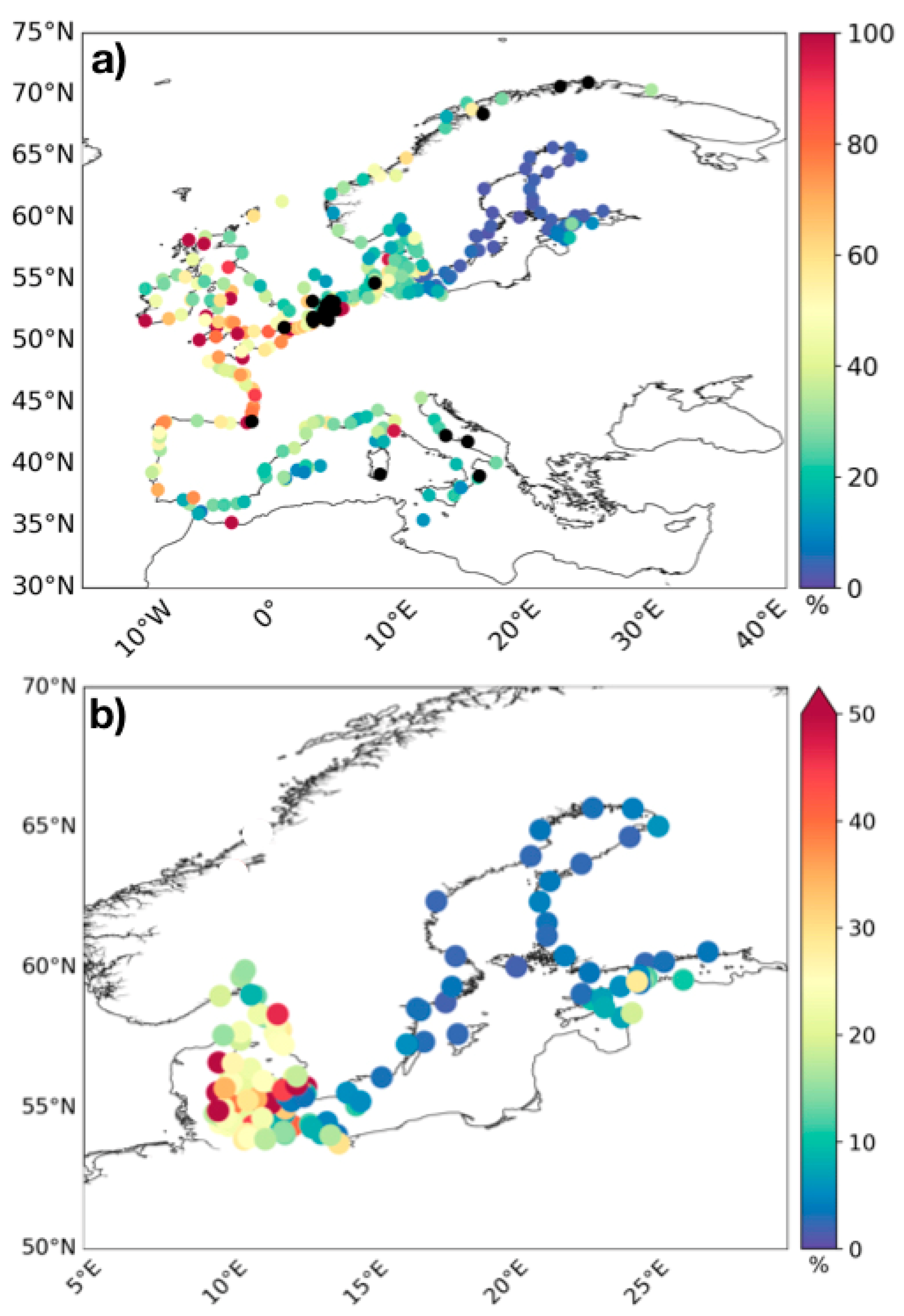
The quality of DUACS Sentinel-3A SAR altimetric 1 Hz in the coastal band of the European Seas, estimated here through comparison with independent tide gauge measurements, revealed a mean RMSD between both datasets lower than 7 cm for the whole region, with mean values ranging around less than 4 cm in the Mediterranean basin and around 10 cm for the NWS region.
Previous works have compared in situ measurements from tide gauges and altimetry data in the European coasts. The tide gauge records from the PSMSL—i.e., [5,20,25] or GLOSS/CLIVAR [23,24,26]—have been mainly considered. The PSMSL repository presents a dense tide gauge network in the European coasts similar to that found in the CMEMS repository, but it is based on monthly average sea level records. [41,42] conducted a regional calibration of the Sentinel-3A data at higher temporal scales by using tide gauge measurements included in the CMEMS repository, but it was focused on the German coasts of the German Bight and of the Baltic Sea. Thus, to our present knowledge, this is the first time that the dense CMEMS tide gauge dataset is used to compare with Sentinel-3A data in the whole European coasts.
The performance of the Sentinel-3A data in the coastal zone of the Gulf of Finland (Baltic Sea) was investigated by [43] through the comparison with tide gauge records from the Estonian Environment Agency. Such records are not included in the CMEMS repository. These authors found an overall RMSD between both datasets of 7 cm based on the inter-comparison with three tide gauge sites. This RMSD is larger than the one obtained here for the Baltic Sea (5.69 cm, Table 2). However, we used 88 tide gauge stations distributed along the whole basin, this allowing a more robust computation.
Ref. [42] compared, among others, the tide gauge sites of Kiel and Warnemünde with the 1 Hz Sentinel-3A data. The tide gauge processing included the tidal correction, whilst DAC and GIA correction were not applied. These authors found a standard deviation of altimeter and tide gauge difference of 3.3 (3.8) cm for the Kiel (Warnemünde) tide gauge station, which is slightly different to those obtained here, 4.0 (6.8) cm, for the same stations. This is probably due to the different tide gauge processing applied and stresses the impact of such processing on the consistency with altimetry data.
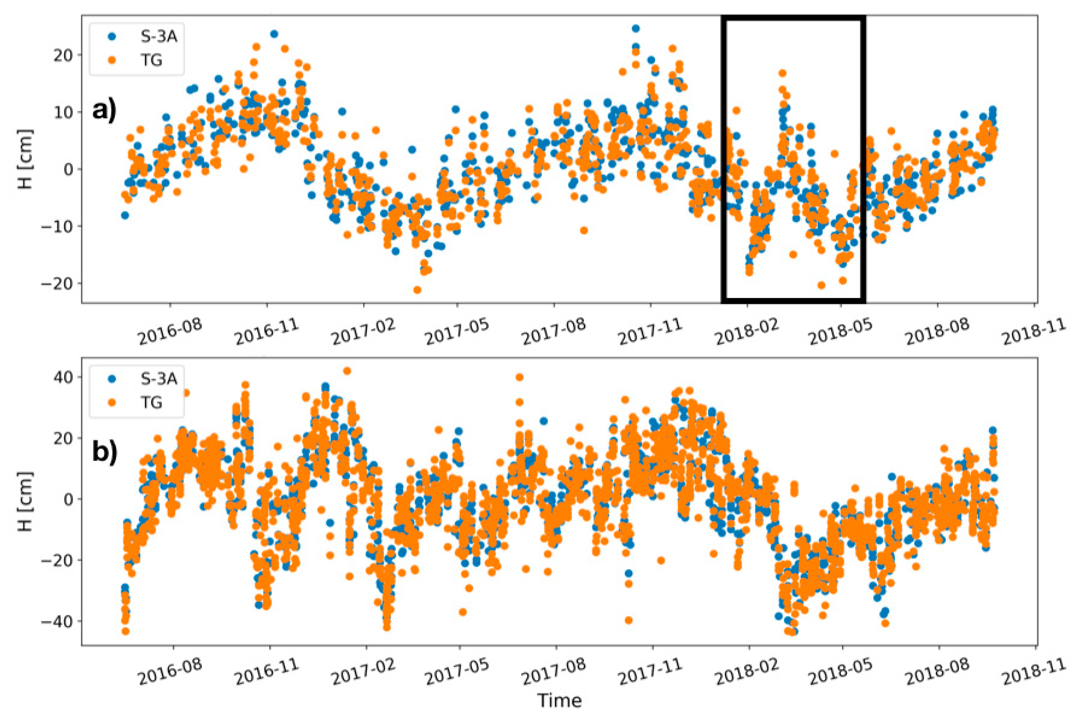
To investigate more in depth the quality of the Sentinel-3A data, a time series for the inter-comparisons conducted in the Mediterranean and Baltic seas is plotted in Figure 5. The tide gauge time series in the former (panel a) shows an annual cycle peaking in October, with an amplitude close to 30 cm. This is an expected result related to the steric effect in the basin that is properly captured by the Sentinel-3A altimetry data. However, this is out of the scope of this paper, because the length of the time series analysed is very short for properly investigating seasonal variability, so in the following we briefly summarise the features found.
A sudden increase in SLA is observed in spring 2018 (black square in Figure 5), promoting a second maximum around March 2018 which is not observed in the previous year, being probably related to some inter-annual variability. This rise in SSH is captured by the Sentinel-3A dataset and also by in situ tide gauge measurements. As a consequence, the annual minimum in SLA observed in previous years in March-April is located in 2018 in May. This signal has not been detected in the other sub-regions investigated by either altimetry or tide gauge measurements.
The tide gauge time series in the Baltic Sea (Figure 5b) show an annual cycle peaking close to December with an amplitude of around 60 cm; this is quite similar to that found for the NWS region (figure not shown). The tide gauge time series exhibit much more inter-annual variability than that of the Mediterranean Sea. The larger seasonal signal observed in the Baltic Sea is attributed to water mass variations within the basin linked to steric changes in the nearby North Atlantic Ocean and river discharges, as well as meteorological forcing, and amplified due to the presence of shallow waters [44].
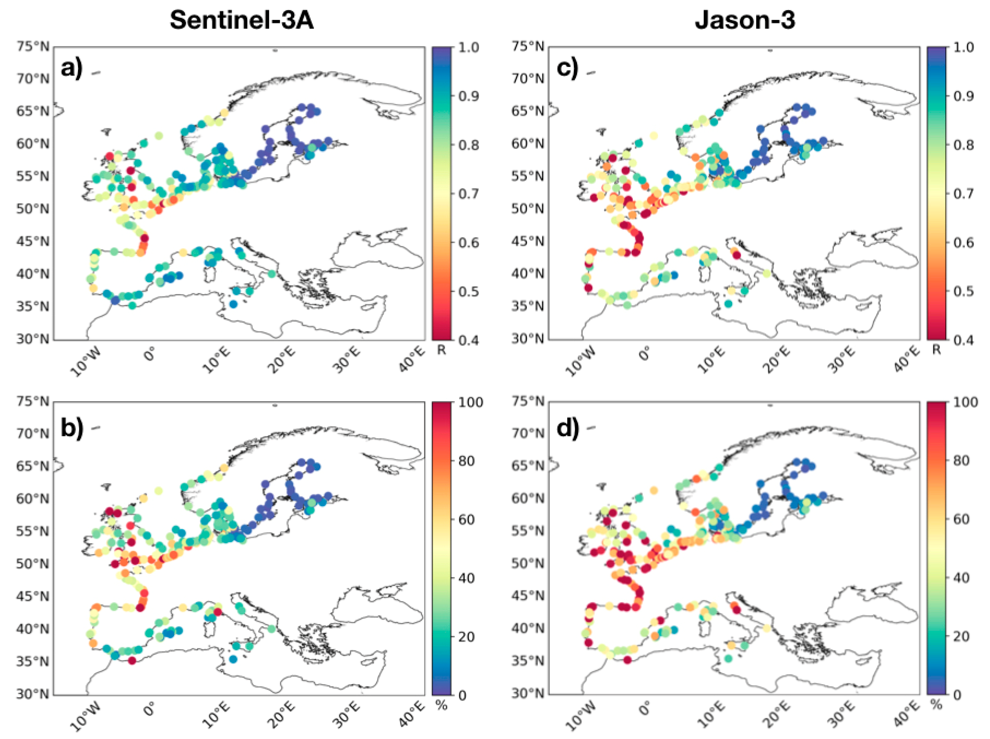
The quality of the Sentinel-3A dataset was also assessed by comparing it with the Jason-3 performance (RMSD and variance) obtained for the inter-comparisons with tide gauges conducted for the entire European coast and the different sub-regions investigated. The results are reported in Table 1 for the whole domain and in Table 2 for the different sub-basins clearly show the superior performance of the Sentinel-3A dataset with respect to Jason-3 in the coastal band in terms of the lower along-track RMSD and lower variance in the differences (altimetry—tide gauge) against the same tide gauges, despite their different ground tracks.
The Sentinel-3A satellite mission improves both the RMSD by 13% and the variance (altimetry—tide gauge) by 25% with respect to the Jason-3 dataset in the European coasts. Figure 6 shows an example of the comparison between Jason-3 and tidal residuals at the tide gauge site of Aranmore (IBI region). A low correlation between both datasets was obtained, thus leading to poorer results than those for the Sentinel-3A mission (figure not shown). Additionally, the mean of the distance between the tide gauge sites and the most correlated altimetry track points used to conduct the inter-comparison reduced by 9% when using the Sentinel-3A altimetry data. This is due to the reduction in the cross-track distance in the Sentinel-3A orbit with respect to Jason-3, which promotes a higher probability of finding a Sentinel-3A track closer to a given tide gauge station. Similar results were found for the different sub-regions investigated.
Lanczos low-pass filtered SLA from Sentinel-3A and Jason-3 were compared with tidal records from the tide gauge sites common to both missions. Overall, the inter-comparisons between the filtered SLA and in situ measurements improved when using the altimetry data from Sentinel-3A in all the regions investigated (Table 6). For the entire European coast, the RMSD was reduced 12% more for the Sentinel-3A satellite mission than for the Jason-3 one. The variance of the differences between both datasets reduced 22% more for the Sentinel-3A mission.
These results confirm that the SRAL instrument better solves the signal in the coastal band than altimeters onboard Jason-3 even when filtered SLA is used. The improvement of Sentinel-3A is higher for the NWS region with respect to the surrounding areas due to poorer performance (not shown) obtained for the Jason-3 mission in the region, which is probably related to the higher significant wave height signal and thus higher noise measurement (1 Hz bump; [17]) for this mission. Similar results were found for the inter-comparison conducted in the Baltic Sea and IBI region, indicating a poorer improvement of Sentinel-3A over Jason-3 in the area. The reduced noise measurement observed in Sentinel-3A contributes to improving the consistency with tide gauge measurements, but it does not explain by itself the improved performances of the Sentinel-3A mission compared to Jason-3.
To further investigate this, the LWE correction applied to the altimetry was checked. We found that the LWE correction diminished the variance of the SLA time series from Sentinel-3A used to compare with tide gauges by 21% in the European coasts (Table 5). This fact translates to better results in terms of the RMSD and variance of the differences (altimetry—tide gauge) when compared with tidal residuals. Similar results were obtained from the Jason-3 dataset. If we compare the outcomes reported in Table 5 for both satellite missions, a larger improvement in statistics was obtained for the Sentinel-3A dataset with respect to Jason-3. This leads to an overall larger impact of LWE correction on SLA from the Sentinel-3A mission.
If the LWE correction is not applied to both altimetry datasets, better results in terms of lower RMSD and variance (altimetry—tide gauge) were still obtained for the Sentinel-3A mission for all the regions investigated (Table 7). If these results are compared with those reported in Table 1 and Table 2, computed from the LWE-corrected SLA, we observe an overall lower improvement in Sentinel-3A over Jason-3 when LWE-uncorrected SLA is used for all the regions investigated except for the IBI region. This fact stresses the higher residual high-frequency LWE for the Sentinel-3A mission shown in Table 5.
The opposite behaviour found in the IBI region—that is, the lightly larger improvement in the Sentinel-3A mission with respect to Jason-3 when using the LWE-uncorrected SLA—could be due to the different location and number of altimetry points used to compare with tide gauges. However, the improvements obtained were only in the range of 1–2%.
These results demonstrate that LWE processing contributes to reducing errors in altimetry, enhancing the consistency between the altimeter and in situ datasets. However, it does not explain alone the better results obtained for the SAR technology in the retrieval of SLA close to the coast. Nonetheless, these outcomes again confirm the better capabilities of SRAL with respect to the altimeters onboard Jason-3 in the retrieval of SLA close to the coast in the European seas.
We have given the reasons why we decided to focus on the reference 1 Hz altimetry data instead of using high-rate (i.e., 20 Hz) SLAs. We realise that the use of high-frequency 20 Hz products could produce better results, and this analysis is in our future plans when these products will be available for the whole oceanographic community.

5. Conclusions

We have performed an assessment of the Sentinel-3A L3 along-track DUACS dataset in the coastal area of the European seas over a period of two and half years from May 2016 to September 2018. This validation was conducted by comparing the equivalent SLAs derived from 6-h sampled tide gauges over the same period in the whole domain and the following sub-regions: the Mediterranean and Baltic Seas and the IBI and NWS regions. Tide gauge records disseminated on CMEMS were used.
The mean value of the RMSD between 1 Hz SLA from Sentinel-3A and tide gauges for the whole European coasts was 6.97 cm. This showed some variability according to the different regions investigated: minimum mean values of 3.41 cm were observed in the Mediterranean Sea and maximum ones (10.72 cm) in the NWS region. These results can be explained by the larger spatio-temporal variability observed in the NWS region with respect to that found in the Mediterranean basin. Non-tidal variance, which is also larger in the former, contributes to the larger RMSD obtained in the NWS region. The assessment was also conducted using altimetry data from Jason-3 for inter-comparison purposes. The Sentinel-3A dataset showed a lower RMSD and variance of the differences (altimetry—tide gauge) in the European coasts.
The impact of the measurement noise on the SRAL instrument was checked by repeating the inter-comparisons but using filtered SLA. The results showed that the variance of altimetry data diminished by 2% when using filtered SLA from Sentinel-3A due to higher frequencies being subtracted from the SLA time series in the filtering procedure. As a consequence, an error 0.3% lower when comparing filtered SLA with tide gauge records with respect to that obtained when using the unfiltered data was obtained. Additionally, the variance of the differences between both datasets reduced by 1% when using the filtered data.
The outcomes from the Jason-3 dataset confirmed the better results obtained from filtered SLA, although much larger discrepancies were found between filtered and unfiltered SLA when comparing with tide gauge records with respect to those obtained for the Sentinel-3A mission. This fact emphasises that the Jason-3 dataset is affected by a higher measurement noise than Sentinel-3A, and also that SRAL instrument onboard the Sentinel-3A mission better solves the signal in the coastal band. This was doubly confirmed from the computations conducted using only filtered SLA from the Sentinel-3A and Jason-3 missions, and also from the analysis of the signal degradation when we approach the coast.
The impact of the LWE correction applied to satellite altimetry was also assessed. The RMSD between the LWE-corrected SLA from the Sentinel-3A and tide gauge records was 10% lower than that obtained when using uncorrected SLA, and the variance of the differences (altimetry—tide gauge) was also reduced by 18%. This is due to a depletion in the variance of SLA due to the LWE correction, which contributes to filtering out part of the residual high-frequency signals not removed after applying other geophysical corrections with respect to uncorrected data. The results for the whole domain and the four sub-regions investigated showed an overall improvement of the Sentinel-3A over Jason-3 when using the LWE-uncorrected SLA for all the regions. Thus, the Sentinel-3A mission still provided better results than the Jason-3 along the European coasts even if the LWE correction was not applied to both.

Author Contributions

Conceptualisation: A.S.-R., M.-I.P., A.P. and Y.F.; altimetry data processing: G.T. and M.-I.P.; tide gauge data processing: A.S.-R. and M.M.; statistical analysis: A.S.-R. and A.P.; manuscript writing: A.S.-R., with inputs from all co-authors. All authors have read and agreed to the published version of the manuscript.

Funding

This study was funded by the Copernicus Marine Environment Monitoring Service (CMEMS) Sea Level Thematic Assembly Centre (SL-TAC). A.P. acknowledges support from the Spanish Research Agency and the European Regional Development Fund (Award no. CTM2016-78607-P). M.M. acknowledges a grant funded by Ministerio de Ciencia e Innovación and Agencia Estatal de Investigación (grant number IED2019-000985-I).

Acknowledgments

This study has been conducted in the frame of the CMEMS SL-TAC and In Situ TAC (INS-TAC) projects. The CMEMS, led by Mercator-Ocean, is based on a distributed model of service production, relying on the expertise of a wide network of participating European organisations involved in operational oceanography. We acknowledge the regional in situ data production centres responsible for the collection and distribution of the tide gauge data used in this study: Puertos del Estado (Spain) for the Iberia-Biscay-Ireland region; HCMR (Greece) for the Mediterranean Sea; IOBAS (Bulgaria) for the Black Sea; IMR (Norway) for the Arctic; SMHI (Sweden) for the Baltic Sea; BSH (Germany) for the North-West Shelves region; Coriolis (France) for the global ocean. This work represents a contribution to CSIC Thematic Interdisciplinary Platform PTI TELEDETECT.

Conflicts of Interest

The authors declare no conflict of interest.

Data Availability

Altimetry datasets are available from the CMEMS web portal (http://marine.copernicus.eu/services-portfolio/access-to-products/, last access: 19 March 2019). Level 2P (L2P) products are distributed by different agencies: NASA, NSOAS, ISRO, ESA, CNES, EUMETSAT. The L3 products for the Sentinel-3A altimetry mission are processed at CLS on behalf of EUMETSAT, funded by the European Union. Tide gauge measurements are available from the CMEMS INS-TAC data repository web portal (www.marineinsitu.eu, last access: 21 May 2019). Tide gauge data are provided by the following regional in situ data production centres: Puertos del Estado (Spain) for the Iberia-Biscay-Ireland region; HCMR (Greece) for the Mediterranean Sea; IOBAS (Bulgaria) for the Black Sea; IMR (Norway) for the Arctic; SMHI (Sweden) for the Baltic Sea; BSH (Germany) for the North-West Shelves region; Coriolis (France) for the global ocean. The ancillary data used to compute the nearest distance to coast of along-track altimetry points are available at the following webpage: https://www.soest.hawaii.edu/pwessel/gshhg/, last access: 5 June 2020).

Appendix A

Table A1. List of tide gauge records with their location and the time period analysed. Bold stations were used in the inter-comparisons with altimetry data, whilst non-bold ones were rejected because they presented spurious data and/or did not keep the selection criteria described in the text.
RegionStation NameLon (°E)Lat (°N)Period Analysed RegionStation NameLon (°E)Lat (°N)Period Analysed
1Baltic SeaAarhus10.2256.1505/2016–09/201832 Heiligenhafen11.0154.3705/2016–09/2018
2 Althagen12.4254.3805/2016–09/201833 Helsinki24.9660.1505/2016–09/2018
3 Arko16.9658.4805/2016–09/201834 Heltermaa23.0558.8705/2016–09/2018
4 Assens9.8855.2705/2016–09/201835 Hesnaes12.1354.8205/2016–09/2018
5 Bagenkop10.6854.7505/2016–09/201836 HirtshalsTG9.9757.605/2016–09/2018
6 Ballen10.6455.8205/2016–09/201837 Hobro9.856.6305/2016–09/2018
7 Bandholm11.4854.8305/2016–09/201838 Holbaek11.7255.7205/2016–09/2018
8 Barhoeft13.0354.4405/2016–09/201839 Hornbaek12.4756.105/2016–09/2018
9 Barseback12.955.7605/2016–09/201840 Hov10.2755.9205/2016–09/2018
10 Bogense10.0855.5705/2016–09/201841 Juelsminde10.0255.7205/2016–09/2018
11 Degerby20.3860.0305/2016–09/201842 Kalix23.165.705/2016–09/2018
12 Dragor12.6855.605/2016–09/201843 Kalkgrund9.8954.8205/2016–09/2018
13 Drogden12.7155.5405/2016–09/201844 Kalvehave12.1755,0005/2016–09/2018
14 Eckernfoerde9.8454.4705/2016–09/201845 Kappeln9.9454.6605/2016–09/2018
15 Eisma26.3159.5705/2016–09/201846 Karrebaeksminde11.6555.1805/2016–09/2018
16 Faaborg10.2555.105/2016–09/201847 Kaskinen21.2162.3405/2016–09/2018
17 Forsmark18.2160.4105/2016–09/201848 Kelnase25.0159.6405/2016–09/2018
18 Fredericia9.7555.5705/2016–09/201849 Kemi24.5265.6705/2016–09/2018
19 Frederikshavn10.5757.4305/2016–09/201850 KielHoltenau10.1654.3705/2016–09/2018
20 Furuogrund21.2364.9205/2016–09/201851 KielLT10.2754.505/2016–09/2018
21 Fynshav9.9855,0005/2016–09/201852 Klagshamn12.8955.5205/2016–09/2018
22 Gedser11.9354.5705/2016–09/201853 Koege12.255.4505/2016–09/2018
23 GoteborgAgnesberg12.0157.7905/2016–09/201854 Korsor11.1355.3305/2016–09/2018
24 GoteborgEriksberg11.9157.705/2016–09/201855 Koserow14,0054.0605/2016–09/2018
25 GoteborgLarjeholm12.0157.7705/2016–09/201856 Kristineberg111.4558.2505/2016–09/2018
26 GoteborgTingstadstunneln11.9957.7205/2016–09/201857 Kungsholmsfort15.5956.1105/2016–09/2018
27 GoteborgTorshamnen11.7957.6805/2016–09/201858 Kungsvik11.1359,0005/2016–09/2018
28 Greifswald13.4554.0905/2016–09/201859 LandsortNorra17.8658.7705/2016–09/2018
29 Grena10.9356.4105/2016–09/201860 Langballigau9.6554.8205/2016–09/2018
30 Hamina27.1860.5605/2016–09/201861 Lehtma22.759.0705/2016–09/2019
31 Hanko22.9859.8205/2016–09/201862 Leppneeme24.8759.5505/2016–09/2019
RegionStation nameLon (°E)Lat (°N)Period analysed RegionStation nameLon (°E)Lat (°N)Period analysed
63 Luebeck10.753.8905/2016–09/201898 Stenungsund11.8358.0905/2016–09/2018
64 Marviken16.8458.5505/2016–09/201899 Stockholm18.0859.3205/2016–09/2018
65 Munalaid24.1258.2305/2016–09/2018100 Stralsund13.154.3205/2016–09/2018
66 Neustadt10.8154.105/2016–09/2018101 Tallinn24.7659.4405/2016–09/2018
67 NordreRose12.6955.6405/2016–09/2018102 Tallinnamadal24.7359.7105/2016–09/2018
68 OlandsNorraUdde17.157.3705/2016–09/2018103 Tejn14.8355.2505/2016–09/2018
69 Onsala11.9257.3905/2016–09/2018104 TimmendorfPoel11.3853.9905/2016–09/2018
70 OscarsborgTG10.659.6805/2016–09/2018105 Travemuende10.8753.9605/2016–09/2018
71 Oskarshamn16.4857.2805/2016–09/2018106 Turku22.160.4305/2016–09/2018
72 Oulu25.4265.0405/2016–09/2018107 Udbyhoej10.356.605/2016–09/2018
73 Paldiski24.0859.3305/2016–09/2018108 Uddevalla11.8958.3505/2016–09/2018
74 Parnu24.4958.3905/2016–09/2018109 Ueckermuende14.0753.7505/2016–09/2018
75 Pietarsaari22.6963.7105/2016–09/2018110 Vaasa21.5763.0805/2016–09/2018
76 Pori21.4661.5905/2016–09/2018111 Vahemadal24.6759.5105/2016–09/2018
77 Porvoo25.6360.2105/2016–09/2018112 Vedbaek12.5755.8505/2016–09/2018
78 Raahe24.4164.6705/2016–09/2018113 Viken12.5856.1405/2016–09/2018
79 Ratan20.963.9905/2016–09/2018114 VikerTG10.9559.0405/2016–09/2018
80 Rauma21.4661.1305/2016–09/2018115 Virtsu23.5158.5805/2016–09/2018
81 Ringhals12.1157.2505/2016–09/2018116 Visby18.2857.6405/2016–09/2018
82 Rodby11.3554.6505/2016–09/2018117 Warnemuende12.154.1705/2016–09/2018
83 Rodvig12.3755.2505/2016–09/2018118 Wismar11.4653.905/2016–09/2018
84 Rohukula23.4258.905/2016–09/2018119 Wolgast13.7754.0405/2016–09/2018
85 Ronne14.6855.105/2016–09/2018120North-West ShelvesA121TG3.8155.405/2016–09/2018
86 Roskilde12.0855.6505/2016–09/2018121AalesundTG6.1562.4705/2016–09/2018
87 Rostock12.1554.0805/2016–09/2018122 AlteWeserTG8.1353.8605/2016–09/2019
88 Sassnitz13.6454.5105/2016–09/2018123 AndenesTG16.1369.3305/2016–09/2020
89 Schleimuende10.0454.6705/2016–09/2018124 AWGTG5.9453.4905/2016–09/2021
90 Simrishamn14.3655.5605/2016–09/2018125 BallumTG8.6955.1305/2016–09/2018
91 SjaellandsOdde11.3755.9705/2016–09/2018126 BergenTG5.3260.405/2016–09/2018
92 Skagen10.5957.7205/2016–09/2018127 BodoeTG14.3967.2905/2016–09/2018
93 Skanor12.8355.4205/2016–09/2018128 BorkumTG6.7553.5605/2016–09/2018
94 Slipshavn10.8355.2805/2016–09/2018129 BoulogneSurMerTG1.5850.7305/2016–09/2018
95 Smogen11.2258.3505/2016–09/2018130 BremerhavenTG8.5753.5405/2016–09/2018
96 Sonderborg9.7854.9205/2016–09/2018131 Brouwershavensegat8TG3.6251.7705/2016–09/2018
97 Spikarna17.5362.3605/2016–09/2018132 BuesumTG8.8654.1205/2016–09/2018
RegionStation nameLon (°E)Lat (°N)Period analysed RegionStation nameLon (°E)Lat (°N)Period analysed
133 CadzandTG3.3851.3805/2016–09/2018168 J61TG5.9453.4905/2016–09/2018
134 CalaisTG1.8750.9705/2016–09/2018169 K13aTG3.2253.2205/2016–09/2018
135 CuxhavenTG8.7253.8705/2016–09/2018170 K141TG3.6353.2705/2016–09/2018
136 D151TG2.9354.3205/2016–09/2018171 KabelvaagTG14.4868.2105/2016–09/2018
137 DagebuellTG8.6954.7305/2016–09/2018172 KeizersveerTG4.8951.7205/2016–09/2018
138 DelfzijlTG6.9353.3305/2016–09/2018173 KornwerderzandTG5.3453.0705/2016–09/2018
139 DenHelderTG4.7552.9705/2016–09/2018174 KrabbersgatsluizenNoordTG5.2852.6905/2016–09/2018
140 DenOeverBinnenTG5.0552.9305/2016–09/2018175 KristiansundTG7.7363.1105/2016–09/2018
141 DenOeverBuitenTG5.0552.9305/2016–09/2018176 L91TG4.8753.5705/2016–09/2018
142 DenOeverTG5.0552.9305/2016–09/2018177 LauwersoogTG6.253.4105/2016–09/2018
143 DordrechtTG4.6751.8205/2016–09/2018178 LemmerTG5.7152.8405/2016–09/2018
144 DunkerqueTG2.3751.0505/2016–09/2018179 Lerwick−1.1460.1505/2016–09/2018
145 EemshavenTG6.8453.4605/2016–09/2018180 LichteilandGoeree1TG3.6751.9305/2016–09/2018
146 EiderSPTG8.8454.2705/2016–09/2018181 ListTG8.4455.0205/2016–09/2018
147 EsbjergTG8.4355.4705/2016–09/2018182 MaloyTG5.1161.9305/2016–09/2018
148 EuroplatformTG3.2852,0005/2016–09/2018183 MausundTG8.6763.8705/2016–09/2018
149 F3platformTG4.7254.8505/2016–09/2018184 NarvikTG17.4368.4305/2016–09/2018
150 HammerfestTG23.6870.6605/2016–09/2018185 NesTG5.7653.4305/2016–09/2018
151 HanstholmTG8.657.1205/2016–09/2018186 NieuwpoortTG2.7351.1505/2016–09/2018
152 Haringvliet10TG3.8651.8605/2016–09/2018187 NorderneyTG7.1653.705/2016–09/2018
153 HarlingenTG5.4153.1805/2016–09/2018188 NorthCormorantTG1.1661.3405/2016–09/2018
154 HarstadTG16.5568.805/2016–09/2018189 Ny-AlesundTG11.9478.9305/2016–09/2018
155 HavnebyTG8.5755.0905/2016–09/2018190 OostendeTG2.9251.2305/2016–09/2018
156 HeimsjoeTG9.163.4305/2016–09/2018191 Oosterschelde11TG3.4851.6405/2016–09/2018
157 HelgeroaTG9.8659,0005/2016–09/2018192 OsloTG10.7359.9105/2016–09/2018
158 HelgolandTG7.8954.1805/2016–09/2018193 OudeSchildTG4.8553.0405/2016–09/2018
159 HoekVanHollandTG4.1251.9805/2016–09/2018194 Q11TG4.1552.9205/2016–09/2018
160 HoernumTG8.354.7605/2016–09/2018195 RibeTG8.6855.3305/2016–09/2018
161 HonningsvaagTG25.9770.9805/2016–09/2018196 RoggebotsluisNoordTG5.8652.5505/2016–09/2018
162 HoutribsluizenNoordTG5.4352.5305/2016–09/2018197 RoompotBuitenTG3.6851.6205/2016–09/2018
163 HuibertgatTG6.453.5705/2016–09/2018198 RorvikTG11.2364.8605/2016–09/2018
164 HusumTG9.0254.4705/2016–09/2018199 ScheveningenTG4.2652.105/2016–09/2018
165 HvideSandeKystTG8.1156,0005/2016–09/2018200 SchiermonnikoogWaddenTG6.253.4705/2016–09/2018
166 IJmondstroompaalTG4.5252.4605/2016–09/2018201 SpijkenisseTG4.3351.8605/2016–09/2018
167 IjmuidenTG4.5652.4605/2016–09/2018202 StavangerTG5.7358.9705/2016–09/2018
RegionStation nameLon (°E)Lat (°N)Period analysed RegionStation nameLon (°E)Lat (°N)Period analysed
203 TerschellingNoordzeeTG5.3353.4405/2016–09/2018238 BarcelonaTG2.1641.3405/2016–09/2018
204 ThyboronKystTG8.2156.7105/2016–09/2018239 CarbonerasTG−1.936.9705/2016–09/2018
205 TorsmindeKystTG8.2156.7105/2016–09/2018240 FormenteraTG1.4238.7305/2016–09/2018
206 TregdeTG7.5558.0105/2016–09/2018241 GandiaTG−0.1538.9905/2016–09/2018
207 TromsoeTG18.9669.6505/2016–09/2018242 IbizaTG1.4538.9105/2016–09/2018
208 TrondheimTG10.3963.4405/2016–09/2018243 MahonTG4.2739.8905/2016–09/2018
209 VardoeTG31.170.3705/2016–09/2018244 MalagaTG−4.4236.7105/2016–09/2018
210 VidaaTG8.6754.9705/2016–09/2018245 MelillaTG−2.9235.2905/2016–09/2018
211 VlakteVdRaanTG3.2451.505/2016–09/2018246 MotrilTG−3.5236.7205/2016–09/2018
212 VlielandHavenTG5.0953.305/2016–09/2018247 PalmadeMallorcaTG2.6439.5605/2016–09/2018
213 VlissingenTG3.651.4505/2016–09/2018248 SaguntoTG−0.2139.6305/2016–09/2018
214 WangeroogeTG7.9353.8105/2016–09/2018249 TarifaTG−5.636.0105/2016–09/2018
215 WestkapelleTG3.4451.5205/2016–09/2018250 TarragonaTG1.2141.0805/2016–09/2018
216 WierumergrondenTG5.9653.5205/2016–09/2018251 ValenciaTG−0.3339.4605/2016–09/2018
217 WilhelmshavenTG8.1553.5105/2016–09/2018252 ANDRATX2.3839.5405/2016–09/2018
218 WittduenTG8.3854.6305/2016–09/2018253 COLONIA-SANT-PERE3.2739.7405/2016–09/2018
219 ZeebruggeTG3.251.3505/2016–09/2018254 POLLENSA3.0939.905/2016–09/2018
220 ZwartsluisTG6.0852.6405/2016–09/2018255 RMN-Ancona13.5143.6205/2016–09/2018
221Med. Sea AjaccioTG8.7641.9205/2016–09/2018256 RMN-Cagliari9.1139.2105/2016–09/2018
222 CenturiTG9.3542.9705/2016–09/2018257 RMN-Catania15.0937.505/2016–09/2018
223 FosSurMerTG4.8943.405/2016–09/2018258 RMN-Crotone17.1439.0805/2016–09/2018
224 IleRousseTG8.9442.6405/2016–09/2018259 RMN-Genova8.9344.4105/2016–09/2018
225 LaFigueiretteTG6.9343.4805/2016–09/2018260 RMN-Imperia28.0243.8805/2016–09/2018
226 MarseilleTG5.3543.2805/2016–09/2018261 RMN-Lampedusa12.635.505/2016–09/2018
227 MonacoTG7.4243.7305/2016–09/2018262 RMN-LeCastella17.0338.9105/2016–09/2018
228 NiceTG7.2943.705/2016–09/2018263 RMN-Livorno10.343.5505/2016–09/2018
229 PortCamargueTG4.1343.5205/2016–09/2018264 RMN-MarinaDiCampo10.2442.7405/2016–09/2018
230 PortFerreolTG6.7243.3605/2016–09/2018265 RMN-Messina15.5638.205/2016–09/2018
231 PortLaNouvelleTG3.0643.0105/2016–09/2018266 RMN-Ortona14.4142.3605/2016–09/2018
232 PortVendresTG3.1142.5205/2016–09/2018267 RMN-Otranto18.540.1505/2016–09/2018
233 SeteTG3.743.405/2016–09/2018268 RMN-Palinuro15.2840.0305/2016–09/2018
234 SolenzaraTG9.441.8605/2016–09/2018269 RMN-ReggioCalabria15.6538.1205/2016–09/2018
235 AlcudiaTG3.1439.8305/2016–09/2018270 RMN-SBenedettoDelTronto13.8942.9605/2016–09/2018
236 AlgecirasTG−5.436.1805/2016–09/2018271 RMN-Sciacca13.0837.505/2016–09/2018
237 AlmeriaTG−2.4836.8305/2016–09/2018272 RMN-Venice12.4345.4205/2016–09/2018
RegionStation nameLon (°E)Lat (°N)Period analysed RegionStation nameLon (°E)Lat (°N)Period analysed
273 RMN-Vieste16.1841.8905/2016–09/2018308 Hinkley−3.1351.2205/2016–09/2018
274 SANT-ANTONI1.338.9805/2016–09/2018309 Holyhead−4.6253.3205/2016–09/2018
275 SA-RAPITA2.9539.3605/2016–09/2018310 Howth−6.0753.3905/2016–09/2018
276Iberian-Biscay-Irish SeasAberdeen−2.0857.1505/2016–09/2018311 HuelvaTG−6.8337.1305/2016–09/2018
277AngletConvergentTG−1.5143.5305/2016–09/2018312 IleDAixTG−1.1746.0105/2016–09/2018
278Aranmore−8.554.9905/2016–09/2018313 Ilfracombe−4.1251.2205/2016–09/2018
279 ArcachonEyracTG−1.1644.6705/2016–09/2018314 Immingham−0.1853.6305/2016–09/2018
280 Ballycotton−8,0051.8305/2016–09/2018315 Killybegs−8.3954.6405/2016–09/2018
281 Ballyglass−9.8954.2505/2016–09/2018316 Kinlochbervie−5.0558.4605/2016–09/2018
282 Bangor−5.6754.6705/2016–09/2018317 LangosteiraTG−8.5343.3505/2016–09/2018
283 Barmouth−4.0352.7205/2016–09/2018318 LaRochelleTG−1.2346.1505/2016–09/2018
284 BayonneBoucauTG−1.5243.5305/2016–09/2018319 LeConquetTG−4.7848.3605/2016–09/2018
285 BilbaoTG−3.0543.3605/2016–09/2018320 LeCrouestyTG−2.947.5405/2016–09/2018
286 BonanzaTG−6.3436.805/2016–09/2018321 LeHavreTG0.1149.4805/2016–09/2018
287 Bournemouth−1.8750.7105/2016–09/2018322 Leith−3.1855.9905/2016–09/2018
288 BrestTG−4.548.3805/2016–09/2018323 LeixoesTG−8.741.1905/2016–09/2018
289 Castletownbere−9.951.6505/2016–09/2018324 LesSablesDOlonneTG−1.7946.505/2016–09/2018
290 CherbourgTG−1.6449.6505/2016–09/2018325 Liverpool−3.0253.4505/2016–09/2018
291 CiboureTG−1.6643.3905/2016–09/2018326 Llandudno−3.8253.3105/2016–09/2018
292 ConcarneauTG−3.9147.8705/2016–09/2018327 Lowestoft1.7552.4705/2016–09/2018
293 CordemaisTG−1.8947.2805/2016–09/2018328 MalinHead−7.3355.3705/2016–09/2018
294 CorunaTG−8.3943.3605/2016–09/2018329 MarinTG−8.6942.4105/2016–09/2018
295 Cromer1.352.9305/2016–09/2018330 Milford−5.0551.7205/2016–09/2018
296 DieppeTG1.0949.9305/2016–09/2018331 Millport−4.955.7505/2016–09/2018
297 Dover1.3251.1205/2016–09/2018332 MimizanTG−1.344.2105/2016–09/2018
298 DublinPort−6.2253.3505/2016–09/2018333 MontoirDeBretagneTG−2.1147.3105/2016–09/2018
299 Dunmore−6.9952.1505/2016–09/2018334 Mumbles−3.9751.5705/2016–09/2018
300 Ferrol2TG−8.2543.4805/2016–09/2018335 NazareTG−9.0739.5905/2016–09/2018
301 FerrolTG−8.3343.4605/2016–09/2018336 Newhaven0.0750.7805/2016–09/2018
302 Fishguard−4.9852.0205/2016–09/2018337 Newlyn−5.5350.105/2016–09/2018
303 GalwayPort−9.0553.2705/2016–09/2018338 Newport−2.9951.5505/2016–09/2018
304 GijonTG−5.743.5605/2016–09/2018339 NorthShields−1.4355,0005/2016–09/2018
305 Harwich1.2951.9505/2016–09/2018340 OuistrehamTG−0.2549.2805/2016–09/2018
306 HerbaudiereTG−2.347.0205/2016–09/2018341 PaimboeufTG−2,0047.2905/2016–09/2018
307 Heysham−2.9254.0305/2016–09/2018342 PenicheTG−9.3739.3505/2016–09/2018
RegionStation nameLon (°E)Lat (°N)Period analysed
343 Plymouth−4.1950.3705/2016–09/2018
344 PortBlocTG−1.0645.5705/2016–09/2018
345 Portbury−2.7351.505/2016–09/2018
346 Portpatrick−5.1254.8405/2016–09/2018
347 Portrush−6.6755.205/2016–09/2018
348 Portsmouth−1.1150.805/2016–09/2018
349 PortTudyTG−3.4547.6405/2016–09/2018
350 RoscoffTG−3.9748.7205/2016–09/2018
351 RoyanTG−1.0345.6205/2016–09/2018
352 SaintMaloTG−2.0348.6405/2016–09/2018
353 SaintNazaireTG−2.247.2705/2016–09/2018
354 SantanderTG−3.7943.4605/2016–09/2018
355 Sevilla2TG−6.0137.3205/2016–09/2018
356 Sheerness0.7551.4505/2016–09/2018
357 SinesTG−8.8937.9505/2016–09/2018
358 SocoaTG−1.6743.405/2016–09/2018
359 StHelier−2.1249.1805/2016–09/2018
360 Stornoway−6.3858.2205/2016–09/2018
361 Tobermory−6.0656.6205/2016–09/2018
362 Ullapool−5.1657.905/2016–09/2018
363 UrtTG−1.343.505/2016–09/2018
364 VianaDoCasteloTG−8.8441.6905/2016–09/2018
365 VigoTG−8.7342.2405/2016–09/2018
366 VillagarciaTG−8.7742.605/2016–09/2018
367 Weymouth−2.4550.6105/2016–09/2018
368 Whitby−0.6254.4805/2016–09/2018
369 Wick−3.0858.4305/2016–09/2018
370 Workington−3.5754.6505/2016–09/2018

Appendix B

Table A2. Tide gauge stations from the CMEMS catalogue in the European Seas showing abnormal variance values in the inter-comparison with altimetry data.
No.Tide Gauge StationLon (°E)Lat (°N)
1AiguillonSurMer−1.3146.33
2BayonnePontBlanc−1.4743.48
3BayonneQuaiDeLesseps−1.4743.49
4Bordeaux−0.5544.86
5Bremen8.7153.12
6Dielette−1.8649.55
7Emden7.1853.33
8Flensburg9.4354.79
9Kampen5.9252.55
10Kobenhavn12.6055.70
11KrabbersgatsluizenZuid5.2852.69
12KrimpenAdLek4.6251.89
13LaCotiniere−1.3245.91
14LePellerin−1.7647.20
15Mangalia28.5943.80
16NantesSalorges−1.5747.20
17NantesUsineBrulee−1.6347.19
18NieuweStatenzijl7.2053.23
19PontDuBrault−1.0846.31
20Rochefort−0.9545.94
21Schleswig9.5654.51
22StMarys−6.3149.91
23StPauli9.9753.54
24Villefranque−1.4643.43

Appendix C

Figure A1 shows the spatial distribution of correlations between tide gauge stations and the Sentinel-3A (left column) and Jason-3 (right column) datasets and the mean square differences between the tide gauge and SLA [variation(tide gauge–altimeter)]/variation(tide gauge). Units are the percent of the tide gauge variance. The common tide gauge stations to both satellite missions have been used for comparison purposes.
Figure A1. Spatial distribution of the correlations (panels a,c) and relative variance reduction between tide gauge and SLA [variation(tide gauge–altimeter)]/variation(tide gauge); units are the percent of the tide gauge variance (panels b,d) for the inter-comparisons between Sentinel-3A (left column) and Jason-3 (right column) with tide gauge time series conducted in the European coasts. Unfiltered SLA and tide gauge stations common to both satellite missions have been used.
Remotesensing 12 03970 g0a1

References

  1. Le Traon, P.Y. From satellite altimetry to Argo and operational oceanography: Three revolutions in oceanography. Ocean Sci. 2013, 9, 901–915. [Google Scholar] [CrossRef] [Green Version]
  2. Couhert, A.; Cerri, L.; Legeais, J.F.; Ablain, M.; Zelensky, P.; Haines, N.P.; Lemoine, B.J.; Bertiger, F.G.; Desai, D.; Otten, M. Towards the 1 mm/y stability of the radial orbit error at regional scales. Adv. Space Res. 2015, 55, 2–23. [Google Scholar] [CrossRef]
  3. Pujol, M.-I.; Faugère, Y.; Taburet, G.; Dupuy, S.; Pelloquin, C.; Ablain, M.; Picot, N. DUACS DT2014: The new multi-mission altimeter data set reprocessed over 20 years. Ocean Sci. 2016, 12, 1067–1090. [Google Scholar] [CrossRef] [Green Version]
  4. Morrow, R.; Carret, A.; Birol, F.; Nino, F.; Valladeau, G.; Boy, F.; Bachelier, C.; Zakardjian, B. Observability of fine-scale ocean dynamics in the northwestern Mediterranean Sea. Ocean Sci. 2017, 13, 13–29. [Google Scholar] [CrossRef] [Green Version]
  5. Taburet, G.; Sanchez-Roman, A.; Ballarotta, M.; Pujol, M.-I.; Legeais, J.-F.; Fournier, F.; Faugere, Y.; Dibarboure, G. DUACS DT2018: 25 years of reprocessed sea level altimetry products. Ocean Sci. 2019, 15, 1207–1224. [Google Scholar] [CrossRef] [Green Version]
  6. Vignudelli, S.; Birol, F.; Benveniste, J.; Fu, L.-L.; Picot, N.; Raynal, M.; Roinard, H. Satellite Altimetry Measurements of Sea Level in the Coastal Zone. Surv. Geophys. 2019, 40, 1319–1349. [Google Scholar] [CrossRef]
  7. Cipollini, P.; Calafat, F.-M.; Jevrejeva, S.; Melet, A.; Prandi, P. Monitoring sea level in the coastal zone with satellite altimetry and tide gauges. Surv. Geophys. 2017, 38, 33–57. [Google Scholar] [CrossRef] [Green Version]
  8. Restano, M.; Passaro, M.; Benveniste, J. New achievements in coastal altimetry. Eos 2018. [Google Scholar] [CrossRef]
  9. Birol, F.; Fuller, N.; Lyard, F.; Cancet, M.; Niño, F.; Delebecque, C.; Fleury, S.; Toublanc, F.; Melet, A.; Saraceno, M.; et al. Coastal applications from nadir altimetry: Example of the X-TRACK regional products. Adv. Space Res. 2017, 59, 936–953. [Google Scholar] [CrossRef]
  10. Ray, R.-D.; Egbert, G.-D.; Erofeeva, S.-Y. Tide predictions in shelf and coastal waters: Status and prospects. In Coastal Altimetry; Vignudelli, S., Kostianoy, A.G., Cipollini, P., Benveniste, J., Eds.; Springer: Berlin, Germany, 2011; pp. 191–216. [Google Scholar]
  11. Bonekamp, H.; Montagner, F.; Santacesaria, V.; Nogueira Loddo, C.; Wannop, S.; Tomazic, I.; O’Carroll, A.; Kwiatkowska, E.; Scharroo, R.; Wilson, H. Core operational Sentinel-3 marine data product services as part of the Copernicus Space Component. Ocean Sci. 2016, 12, 787–795. [Google Scholar] [CrossRef] [Green Version]
  12. Raney, R.K. The delay/Doppler radar altimeter. IEEE Trans. Geosci. Remote Sens. 1998, 36, 1578–1588. [Google Scholar] [CrossRef]
  13. Heslop, E.-E.; Sánchez-Román, A.; Pascual, A.; Rodríguez, D.; Reeve, K.-A.; Faugère, Y.; Raynal, M. Sentinel-3A views ocean variability more accurately at finer resolution. Geophys. Res. Lett. 2017, 44. [Google Scholar] [CrossRef] [Green Version]
  14. Peng, F.; Deng, X. Validation of Sentinel-3A SAR mode sea level anomalies around the Australian coastal region. Remote Sens. Environ. 2020, 237, 111548. [Google Scholar] [CrossRef]
  15. Dinardo, S.; Fenoglio-Marc, L.; Buchhaupt, C.; Becker, M.; Scharroo, R.; Fernandes, M.J.; Benveniste, J. Coastal SAR and PLRM altimetry in German Bight and west Baltic Sea. Adv. Space Res. 2018, 62, 1371–1404. [Google Scholar] [CrossRef]
  16. AVISO+, Along-Track Level-2+ (L2P) SLA Product Handbook, v1.0. 2017. Available online: https://www.aviso.altimetry.fr/fileadmin/documents/data/tools/hdbk_L2P_all_missions_except_S3.pdf (accessed on 6 July 2020).
  17. Dibarboure, G.; Pujol, M.-I. Improving the quality of Sentinel-3A with a hybrid mean sea surface model, and implications for Sentinel-3B and SWOT. Adv. Space Res. 2019. [Google Scholar] [CrossRef]
  18. CMEMS. QUID for Sea Level TAC DUACS Products. 2020. Available online: https://resources.marine.copernicus.eu/documents/QUID/CMEMS-SL-QUID-008-032-062.pdf (accessed on 25 August 2020).
  19. Valladeau, G.; Legeais, J.-F.; Ablain, M.; Guinehut, S.; Picot, N. Comparing Altimetry with Tide Gauges and Argo Profiling Floats for Data Quality Assessment and Mean Sea Level Studies. Mar. Geod. 2012, 35, 42–60. [Google Scholar] [CrossRef]
  20. Wöppelmann, G.; Marcos, M. Vertical land motion as a key to understanding sea level change and variability. Rev. Geophys. 2016, 54, 64–92. [Google Scholar] [CrossRef] [Green Version]
  21. PSMSL. Permanent Service for Mean Sea Level: “Tide Gauge Data”. 2016. Available online: http://www.psmsl.org/data/obtaining/ (accessed on 10 July 2020).
  22. SALP Annual Report (2017) of Mean Sea Level Activities, Edn. 1.0. 2018. Available online: https://www.aviso.altimetry.fr/fileadmin/documents/calval/validation_report/SALP-RP-MA-EA-23189-CLS_AnnualReport_2017_MSL.pdf (accessed on 4 October 2018).
  23. Pascual, A.; Faugère, Y.; Larnicol, G.; Le Traon, P.-Y. Improved description of the ocean mesoscale variability by combining four satellite altimeters. Geophys. Res. Lett. 2006, 33, L02611. [Google Scholar] [CrossRef] [Green Version]
  24. Pascual, A.; Boone, C.; Larnicol, G.; Le Traon, P.Y. On the quality of real-time altimeter gridded fields: Comparison with in situ data. J. Atmos. Ocean. Technol. 2009, 26, 556–569. [Google Scholar] [CrossRef] [Green Version]
  25. Marcos, M.; Pascual, A.; Pujol, I. Improved satellite altimeter mapped sea level anomalies in the Mediterranean Sea: A comparison with tide gauges. Adv. Space Res. 2015, 56, 596–604. [Google Scholar] [CrossRef] [Green Version]
  26. Pascual, A.; Pujol, M.I.; Larnicol, G.; Le Traon, P.-Y. Mesoscale mapping capabilities of multisatellite altimeter missions: First results with real data in the Mediterranean Sea. J. Mar. Syst. 2007, 65, 190–211. [Google Scholar] [CrossRef]
  27. Caldwell, P.C.; Merrifield, M.A.; Thompson, P.R. Sea Level Measured by Tide Gauges from Global Oceans—The Joint Archive for Sea Level Holdings; (NCEI Accession 0019568); Version 5.5; NOAA National Centers for Environmental Information: Asheville, NC, USA, 2015. [Google Scholar] [CrossRef]
  28. Codiga, D.L. Unified Tidal Analysis and Prediction Using the UTide Matlab Functions; Technical Report 2011-01; Graduate School of Oceanography, University of Rhode Island: Narragansett, RI, USA, 2011; p. 59. [Google Scholar]
  29. Carrère, L.; Lyard, F. Modeling the barotropic response of the global ocean to atmospheric wind and pressure forcing—Comparisons with observations. Geophys. Res. Lett. 2003, 30, 1275. [Google Scholar] [CrossRef] [Green Version]
  30. Carrère, L.; Faugère, Y.; Bronner, E.; Benveniste, J. Improving the dynamic atmospheric correction for mean sea level and operational applications of altimetry. In Proceedings of the 2011 Ocean Surface Topography Science Team (OSTST) meeting, San Diego, CA, USA, 19–21 October 2011. [Google Scholar]
  31. Peltier, W.R. Postglacial Variations in the Level of the Sea: Implications for Climate Dynamics and Solid-Earth Geophysics. Rev. Geophys. 1998, 36, 603–689. [Google Scholar] [CrossRef]
  32. Peltier, W.R. Global Glacial Isostasy and the Surface of the Ice-Age Earth: The ICE-5G(VM2) model and GRACE. Ann. Rev. Earth Planet. Sci. 2004, 32, 111–149. [Google Scholar] [CrossRef]
  33. Sánchez-Román, A.; Ruiz, S.; Pascual, A.; Mourre, B.; Guinehut, S. On the mesoscale monitoring capability of Argo floats in the Mediterranean Sea. Ocean Sci. 2017, 13, 223–234. [Google Scholar] [CrossRef] [Green Version]
  34. Efron, B.; Tibshirani, R. Bootstrap Methods for Standard Errors, Confidence Intervals, and Other Measures of Statistical Accuracy. Stat. Sci. 1986, 1, 54–77. Available online: https://projecteuclid.org/euclid.ss/1177013815 (accessed on 2 July 2020). [CrossRef]
  35. Wessel, P.; Smith, W.H.F. A Global Self-consistent, Hierarchical, High-resolution Shoreline Database. J. Geophys. Res. 1996, 101, 8741–8743. [Google Scholar] [CrossRef] [Green Version]
  36. Von Schuckmann, K.; Le Traon, P.-Y.; Smith, N.; Pascual, A.; Brasseur, P.; Fennel, K.; Djavidnia, S.; Aaboe, S.; Fanjul, E.A.; Autret, E.; et al. Copernicus Marine Service Ocean State Report. J. Oper. Ocean. 2018, 11, S1–S142. [Google Scholar] [CrossRef] [Green Version]
  37. Raynal, M.; Labroue, S.; Orsztynowicz, M.; Picot, N.; Guillot, A.; Boy, F. Sentinel-6A Delay Doppler Processing: Assessment over the Global Ocean. In Proceedings of the SAR Workshop 2016, La Rochelle, France, 31 October–4 November 2016. [Google Scholar]
  38. Moreau, T.; Cadier, E.; Boy, F.; Aublanc, J.; Rieu, P.; Raynal, M.; Labroue, S.; Thibaut, P.; Dibarboure, G.; Picot, N.; et al. High-performance altimeter Doppler processing for measuring sea level height under varying sea state conditions. Adv. Space Res. 2020. Under review. [Google Scholar]
  39. Gommenginger, C.; Thibaut, P.; Fenoglio-Marc, L.; Quartly, G.; Deng, X.L.; Gómez-Enri, J.; Challenor, P.; Gao, Y.G. Retracking altimeter waveforms near the coasts. In Coastal Altimetry; Vignudelli, S., Kostianoy, A., Cipollini, P., Benveniste, J., Eds.; Springer: Berlin, Germany, 2011; pp. 61–101. [Google Scholar] [CrossRef]
  40. CMEMS INS QUID for Near Real Time IN SITU Products. 2019. Available online: http://marine.copernicus.eu/documents/QUID/CMEMS-INS-QUID-013-030-036.pdf (accessed on 6 July 2020).
  41. Fenoglio, L.; Dinardo, S.; Uebbing, B.; Buchhaupt, C.; Scharroo, R.; Kusche, J.; Benveniste, J. Water level retreival from Sentinel-3. In Proceedings of the 5th S3VT Meeting, Frascati, Rome, Italy, 7–9 May 2019. [Google Scholar]
  42. Fenoglio, L.; Dinardo, S.; Buchhaupt, C.; Uebbing, B.; Scharroo, R.; Kusche, J.; Becker, M.; Benveniste, J. Calibrating CryoSat-2 and Sentinel-3A Sea Surface Heights along the German coast. In Fiducial Reference Measurements for Altimetry. International Association of Geodesy Symposia; Mertikas, S., Pail, R., Eds.; Springer: Berlin, Germany, 2019; Volume 150, ISBN 978-3-030-39437-0. [Google Scholar] [CrossRef]
  43. Birgiel, E.; Ellmann, A.; Delpeche-Ellmann, N. Examining the Performance of the Sentinel-3 Coastal Altimetry in the Baltic Sea Using a Regional High- Resolution Geoid Model. In Proceedings of the 2018 Baltic Geodetic Congress (Geomatics), University of Warmia and Mazury in Olsztyn, Olsztyn, Poland, 21–23 June 2018. [Google Scholar]
  44. Stramska, M.; Kowalewska-Kalkowska, H.; Świrgon, M. Seasonal variability of the Baltic Sea level. Oceanologia 2013, 55, 787–807. Available online: https://www.sciencedirect.com/science/article/pii/S0078323413500406 (accessed on 21 October 2020). [CrossRef]
Figure 1. Flowchart of the Data Unification and Altimeter Combination System (DUACS) procedure applied to altimetry data and the processing of the tide gauge data used to compare with altimetry.
Remotesensing 12 03970 g001
Figure 2. Location of the 370 tide gauges of the global product in the Copernicus catalogue along the European coasts and the western Mediterranean Sea used to compare with altimetry data after applying the selection criteria described in the text. Colours indicate the length of the time series of the concurrent tide gauge data and altimeter data. The black squares denote the sub-regions used for the inter-comparisons (see the text for details).
Remotesensing 12 03970 g002
Figure 3. Spatial distribution of the mean square differences between the tide gauge and altimetry sea level from Sentinel-3A in the European coasts (panel (a)). Black dots denote the location of the tide gauge sites rejected from the computation according with the selection criteria described in the text. Panel (b) shows a detailed view of the Baltic Sea region. Sea Level Anomaly (SLA) measurements without filtering have been used. Units are the percent of tide gauge variance.
Remotesensing 12 03970 g003
Figure 4. Spatial distribution of the variance (cm2) of Long Wavelength Error (LWE) correction applied on SLA measurements (without filtering) from the Sentinel-3A dataset along the European coasts. Black dots denote the location of the tide gauge sites rejected from the computation according with the selection criteria described in the text.
Remotesensing 12 03970 g004
Figure 5. Time series of SLA (cm) obtained from the Sentinel-3A most correlated track points (blue dots) and tidal residuals (orange dots) time series at each station site for (a) the Mediterranean basin and (b) the Baltic Sea. Black square denotes the time period showing a second maximum in 2018 for SLA. The mean value of each time series has been subtracted for comparison purposes.
Remotesensing 12 03970 g005
Figure 6. Time series of SLA (cm) obtained from the Jason-3 most correlated track points (dotted purple line) and tidal residuals (dotted black line) time series at the tide gauge site of Aranmore located at coordinates: −8.5° E/54.99° N (northern cost of Ireland—IBI region). The mean value of each time series has been subtracted for comparison purposes.
Remotesensing 12 03970 g006
Table 1. Inter-comparison of the satellite altimetry and tide gauge data from the European coasts in terms of the RMSD (cm) and variance (cm2) of the differences between both datasets. The number of tide gauge stations used in the comparison, the mean distance between tide gauges and the most correlated along-track altimetry points, and the number of total data pairs (altimetry-tide gauge) used in the computation are displayed. The common tide gauge stations for the Sentinel-3A and Jason-3 satellite missions were used. Values in parenthesis show the uncertainties (error bars) computed for the RMSD and variance from the bootstrap method using 103 iterations. Finally, the improvement (%) of the Sentinel-3A data in comparison with tide gauges in terms of lower RMSD, lower variance of the differences (altimetry-tide gauge), and lower mean distance between the most correlated altimetry point and tide gauges with respect to Jason-3 is also displayed. SLA measurements without filtering have been used.
European CoastsSentinel-3AJason-3Improvement
RMSD (cm)6.89 (0.17)7.97 (0.21)13%
var TG (cm2)150 (6)138 (5)
var ALT (cm2)124 (5)117 (5)
var TG-ALT (cm2)47 (3)64 (3)25%
data pairs60376172
stations270270
distance TG (km) 79 ± 33 87 ± 339%
Table 2. The same as Table 1 but for the different sub-regions investigated: Mediterranean Sea, Iberian-Biscay-Irish (IBI) region, North-West Shelves (NWS) region, and Baltic Sea.
Sub-RegionsSentinel-3AJason-3Improvement S-3A
Mediterranean Sea
RMSD (cm)3.47 (0.22)4.49 (0.28)23%
var TG (cm2)53 (5)46 (4)
var ALT (cm2)52 (5)49 (4)
var TG-ALT (cm2)12 (1)20 (3)40%
data pairs743836
stations3838
distance TG (km) 67 ± 3074 ± 409%
IBI region
RMSD (cm)6.62 (0.30)7.31 (0.28)9%
var TG (cm2)72 (5)63 (4)
var ALT (cm2)56 (4)51 (4)
var TG-ALT (cm2)44 (4)53 (4)18%
data pairs19271920
stations8181
distance TG (km)80 ± 3089 ± 3310%
NWS region
RMSD (cm)10.31 (0.53)12.22 (0.60)15%
var TG (cm2)268 (22)264 (20)
var ALT (cm2)201 (18)185 (16)
var TG-ALT (cm2)106 (11)149 (14)29%
data pairs12561416
stations5555
distance TG (km)84 ± 35101± 2717%
Baltic Sea
RMSD (cm)5.69 (0.28)6.24 (0.28)9%
var TG (cm2)217 (13)199 (12)
var ALT (cm2)190 (11)184 (12)
var TG-ALT (cm2)32 (3)39 (3)17%
data pairs19401856
stations8888
distance TG (km)78 ± 33 78 ± 31---
Table 3. The same as Table 1 but for the inter-comparison using Lanczos low-pass filtered SLA and SLA measurements without filtering for the Sentinel-3A and Jason-3 satellite missions. Common tide gauge stations for each satellite mission have been used.
European CoastsSentinel-3AImprov. Filtered S-3AJason-3Improv. Filtered J-3
UnfilteredFilteredUnfilteredFiltered
RMSD (cm)6.97 (0.19)6.95 (0.19)0.3%8.72 (0.25)8.52 (0.25)2.3%
var TG (cm2)149 (5) 146 (6)
var ALT (cm2)121(7)119 (7)−2%121 (5)114 (5)−6%
var TG-ALT (cm2)49 (3)48 (3)1%76 (4)72 (4)5%
data pairs7119 6228
stations340 277
distance TG (km)80 ± 36 87 ± 34
Table 4. The same as Table 1 but for the inter-comparison using the altimetry closest track point to coast (ctp) and the most correlated altimetry point (mcp) with tide gauge records computed along the satellite track of ctp (see text for details) for the twenty-seven common tide gauge stations showing a similar distance with the altimetry ctp for Sentinel-3A and Jason-3 (a maximum difference of 1 km is allowed). The distance (km) of mcp and ctp to both tide gauges (TG) and coast and the degradation (in percentage) of the altimetry signal, computed as the differences between mcp and ctp, are also shown.
European CoastsSentinel-3AJason-3Degrad. S-3ADegrad. J-3
mcpctpmcpctp
RMSD (cm)6.787.957.918.7415%10%
var TG (cm2)173172
var ALT (cm2)1211271251395%10%
var TG-ALT (cm2)62808110122%20%
distance TG (km)6046877523%14%
distance coast (km)13.55.112.25.462%56%
data pairs456442
stations27
Table 5. Inter-comparison of the LWE-corrected and -uncorrected SLA from the Sentinel-3A and Jason-3 satellite missions and tide gauge data in the European coasts in terms of the RMSD (cm) and variance (cm2) of the differences between the datasets. The number of tide gauge stations used in the comparison, the mean distance between tide gauges and the most correlated along-track altimetry points, and the number of total data pairs (altimetry-tide gauge) used in the computation are displayed. The common tide gauge stations for each satellite mission have been used. Values in parentheses show the uncertainties (error bars) computed for the RMSD and variance from the bootstrap method using 103 iterations. Finally, the improvement (%) of the LWE-corrected SLA data from Sentinel-3A and Jason-3 in the comparison with tide gauges, in terms of the lower RMSD and lower variance of the differences (altimetry-tide gauge) with respect to the LWE-uncorrected SLA data, is also displayed. SLA measurements without filtering have been used.
European CoastsSentinel-3AImprov. Corrected S3AJason-3Improv. Corrected J3
LWE CorrectedLWE UncorrectedLWE CorrectedLWE Uncorrected
RMSD (cm)6.94 (0.19)7.67 (0.20)10%8.61 (0.24)8.84 (0.25)3%
var TG (cm2)148 (5)159 (6) 145 (6)147 (6)
var ALT (cm2)120 (5)152 (6)−21%120 (5)144 (6)−16%
var TG-ALT (cm2)48 (3)59 (3)18%74 (4)78 (4)5%
data pairs7170 6386
stations337 278
distance TG (km) 80 ± 33 87 ± 33
Table 6. Summary of the improvements (%) of the Sentinel-3A mission in comparison with tide gauges in terms of the lower RMSD, lower variance of the differences (altimetry—tide gauge), and lower mean distance between the most correlated altimetry point and tide gauges with respect to Jason-3 in the European coasts and the different sub-regions investigated. The analysis is similar to that shown in Table 1 and Table 2 (last column), but using filtered SLA data.
European CoastsMed. SeaIBI RegionNWS RegionBaltic Sea
% reduction in RMSD12%13%9%12%9%
% reduction in variance
(TG-ALT)
22%24%17%22%17%
% reduction in distance to TG7%---8%14%---
Table 7. Summary of the improvements (%) of the Sentinel-3A mission in the comparison with tide gauges in terms of the lower RMSD, lower variance of the differences (altimetry—tide gauge), and lower mean distance between the most correlated altimetry point and tide gauges with respect to Jason-3 in the European coasts, and the different sub-regions investigated. The analysis is similar to that shown in Table 1 and Table 2 (last column) but using LWE-uncorrected SLA data.
European CoastsMed. SeaIBI RegionNWS RegionBaltic Sea
% reduction in RMSD7%14%10%3%7%
% reduction in variance (TG-ALT)13%24%19%6%14%
% reduction in distance to TG8%13%15%---13%
Publisher’s Note: MDPI stays neutral with regard to jurisdictional claims in published maps and institutional affiliations.

