About Validation-Comparison of Burned Area Products
by
 , ,
, ,
Germán M. Valencia
1,2,* ,
,
Jesús A. Anaya
2,
Éver A. Velásquez
3,
Rubén Ramo
4 and
Francisco J. Caro-Lopera
3 1
Facultad de Ingenierías, Universidad de San Buenaventura, Medellín 050010, Colombia
2
Facultad de Ingenierías, Universidad de Medellín, Medellín 050026, Colombia
3
Facultad de Ciencias Básicas, Universidad de Medellín, Medellín 050026, Colombia
4
Departamento de Geología, Geografía y Medio Ambiente, Universidad de Alcalá, Colegios 2, 28801 Alcalá de Henares, Spain
*
Author to whom correspondence should be addressed.
Remote Sens. 2020, 12(23), 3972; https://doi.org/10.3390/rs12233972
Submission received: 27 July 2020
/
Revised: 28 August 2020
/
Accepted: 5 September 2020
/
Published: 4 December 2020
Abstract
:This paper proposes a validation-comparison method for burned area (BA) products. The technique considers: (1) bootstrapping of scenes for validation-comparison and (2) permutation tests for validation. The research focuses on the tropical regions of Northern Hemisphere South America and Northern Hemisphere Africa and studies the accuracy of the BA products: MCD45, MCD64C5.1, MCD64C6, Fire CCI C4.1, and Fire CCI C5.0. The first and second parts consider methods based on random matrix theory for zone differentiation and multiple ancillary variables such as BA, the number of burned fragments, ecosystem type, land cover, and burned biomass. The first method studies the zone effect using bootstrapping of Riemannian, full Procrustes, and partial Procrustes distances. The second method explores the validation by using distance permutation tests under uncertainty. The results refer to Fire CCI 5.0 with the best BA description, followed by MCD64C6, MCD64C5.1, MCD45, and Fire CCI 4.1. It was also found that biomass, total BA, and the number of fragments affect the BA product accuracy.
1. Introduction
Burning of biomass is one of the main sources of aerosol and greenhouse gas emissions in the atmosphere [1]. This influences strongly carbon cycles and plant succession processes [2]. According to Giglio et al. [3], each year on average 348 million hectares of biomass are burned around the world. For the most part, this quantity is detected by means of satellite remote sensing in the optical region: red (620–670 nm), NIR (1230–1250 nm), and SWIR (2105–2155 nm) [4]. However, in geographical areas like the tropics, the identification of burning on this spectral zone is complex due to extensive cloud cover [5] and the size of the fires [6], probably due to the moisture content in the forests [7], and in the case of the savannas, the rapid movement (and short-lived) of fire and relatively low fuel levels [8], which limit the detection of fires. These elements have an impact on emissions estimates and on reports of burned area (BA). Chuvieco et al. [9] reported a greater amount of area burned in the world compared to those of Giglio et al. [3] and estimated that between 324 and 416 million hectares are burned annually around the world.
Tropical regions have the largest deposits of aboveground biomass [10,11,12]. They also involve a high percentage of the biomass burned in the world [13], contributing to the main concentrations of carbon emissions in the atmosphere since 1750 to 2015 [14]. Therefore, assessing the accuracy of BA products in tropical regions is required in order to monitor vegetation changes and the greenhouse gas emissions.
Several validation analyses have been proposed in different regions around the world [2,15,16]. Specifically, in tropical regions of Northern Hemisphere South America (NHSA) and Northern Hemisphere Africa (NHAF) the attention has focused only on validation of tropical savannas [17]. However, the analysis of other ecosystems should provide new insights about the performance of the burned area (BA) products. Additionally, the large omission of BA detection in tropical regions (35% of the global BA values [6]) is known to be related to the short duration of fires [18], or cloud cover [7], or forest phytophysiognomies [19].
Chu & Guo et al. [20] mention the problems in the automation of cartography and modeling of BA detection, attributed mainly to the complexity of the variables involved. The fire regime, climatic and environmental conditions, and the different optical sensors influence the quality of the products. Indeed, Palomino & Anaya [21] presented some of these difficulties in their validation study of the MCD45 BA product, carried out in the tropical savannah of Northern South America. They argued that the spatial resolution, the large cloud content and the type of vegetation are some of the problems faced when mapping burned areas. In the same way, Roy et al. [22] compared the MCD45 BA product with MOD14 hotspots at a global level. They found that difficulties are associated with environmental variables such as clouds, aerosols, vegetation type, fragment distribution, spatial sensor resolution, temporal resolution, and sensor passing time. Accordingly, these elements influence the size of the burned areas detected by the global products and consequently the data accuracy.
Two techniques are used for the validation of BA products. The first technique involves global concordance measurements via error matrix [23]: bias scaled relative to the reference burning area, Dice coefficient, commission errors, omission errors [2,15,24]. Another method considers goodness of fit in least-squares models (R2) [9,25,26,27,28,29,30,31,32]. Each method has constraints to be considered in the applications. The least squares model requires verification of the Gauss–Markov theorem. If the regression diagnostics fail, then the inference of the linear model and the common R2 cannot be used for supporting validation [33,34,35]. Moreover, to assume that diagnoses are fulfilled by only taking into account a high R2 but not interception, it is not in agreement with the Gauss-Markov theorem based on a model with intercept [36]. It is difficult to set a priori that a least square linear validation model has intercept, because we expect that an ideal BA product must match perfectly with reference data; the ideal product should report zero omissions and commissions errors and equal proportions of burned and non-burned pixels in the reference data [37,38,39]. Other difficult situations involve sample scatterplots of separated clusters and cones with vertex at the origin [40]. Additionally, the linear model of a BA product versus reference data demands an independent predictor (reference data). Otherwise, the Gauss–Markov theorem cannot be applied. A recent alternative for dealing with such problem involves a statistical calibration with bootstrapping and a Simulation Extrapolation method (SIMEX) [41].
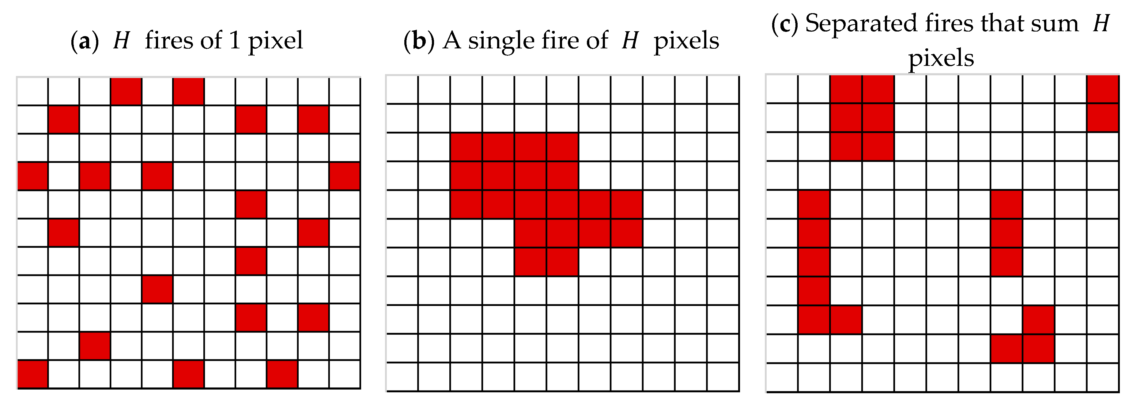
The error matrix collects the agreement, disagreement, omission and commission proportions with reference. However, different fire morphologies reported by reference data provide the same error matrix as is shown in the Figure 1. Then, considering the number of burned fragments and the associated statistics can enrich the accuracy assessment. Further analysis can consider ecosystem multiple variables, transportation and correlation of the fragments.
This work proposes a method for validation and comparison of five BA products with reference data by including the location, biomass, land cover, fire size, and the number of fires in 44 scenes of the tropics in Northern Hemisphere South America (NHSA) and Northern Hemisphere Africa (NHAF). The method includes two parts: (1) a comparison and validation of BA products by bootstrapping; (2) randomness and permutation tests for validation of BA products.
2. Materials and Methods
2.1. Study Area
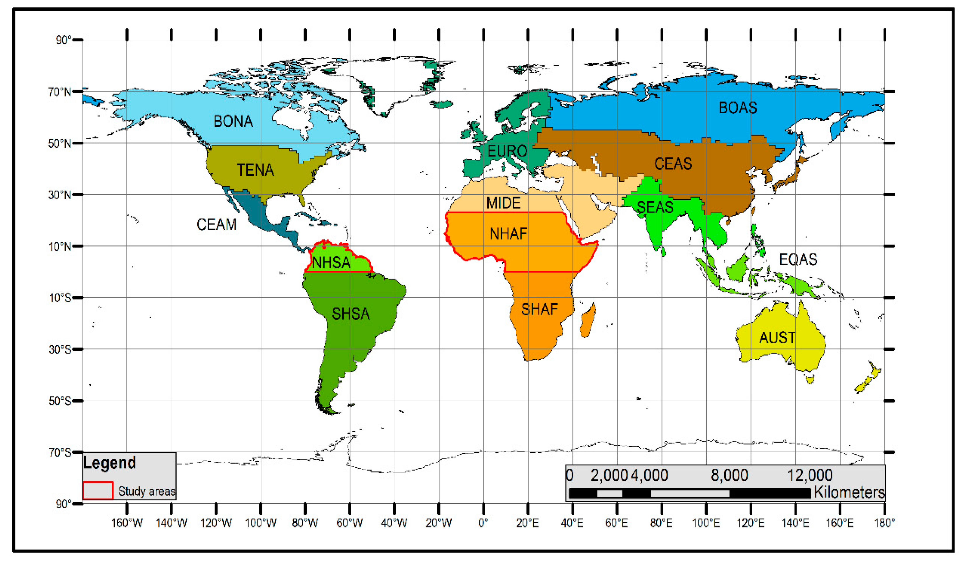
Giglio et al. [42] divided the continents into regions of fire using a study of five temporal metrics as shown in Figure 2. In this paper we will focus on two regions: Northern Hemisphere South America (NHSA) and Northern Hemisphere Africa (NHAF). Both regions are highly affected by fires [43,44,45,46,47,48].
Contributions about sample size and error for validation scenes can be found in Supplementary Material Section S1.1. Likewise, the location of sample scenes are described in Supplementary Material Section S1.2. This information was not included in the paper to avoid any confusion with the main purpose of validation-comparison of BA products. However, the addressed methods given in the Supplementary Material consider innovations that an interested reader can use in similar verification works. For example, they hold for quality validation of cartographic products and accuracy assessment of land cover products.
2.2. Data
2.2.1. Reference Data
In 2009, Boschetti, et al. [24], defined a standard protocol that is used by the CEOS Cal-Val (attached to the CEOS-WGCV) for the process of validating the quality of the cartographic products. An adjustment to this protocol was implemented to restrict the fire perimeters for the years 2007–2008, a period with a significant increment of fires in NHSA and NHAF regions according to report emissions GFED model (Global Fire Emissions Database, see https://www.globalfiredata.org/). In Supplementary Material (SM) Section S1.3, we propose a method for processing the reference data with a hybrid method combining the BAMS model, based on LANDSAT 5 (TM) and 7 (ETM+) [50], with cloud masking, cloud shadows and water masks based on temporal stability proposed by Valencia et al. [40]. The last one was based on the LEDAPS model by Masek et al. [51]. The results were verified with a good level of confidence according to Claverie et al. [52].
The addressed hybrid method derived by Valencia et al. [37] is based on the fact that the LEDAPS cloud mask is more accurate than BAMS cloud mask (see SM Section S1.3). Moreover, it also considers a validation of the seeds obtained by the BAMS model, because some polygons can appear as burned areas due to changes in soil moisture.
2.2.2. BA Products Considered for Validation and Comparison
The BA products evaluated in this study (Table 1) include: MCD64 Collections 5 and 6, derived from the NASA MODIS Land science Team; MCD45; Fire-CCI 4.1, and 5.0, from the European Space Agency.
2.2.3. Ancillary Information
The analysis of this work includes quantitative and qualitative variables in order to describe the ecosystems and the BA phenomenon. We consider the spatial location of the LANDSAT scenes (WRS2 path and row), land cover, continent, biomass, average fire size, and number of burned fragments. Additionally, vegetation cartographic layers studied by Avitabile et al. [10], Olson et al. [54], and ESA [55] were also included in our research (see Table 2).
2.3. Statistical Methods for Validation and Comparison of BA Products
In the validation process, the error matrix and the associated statistics provide percentages of omission, commission, agreement and discrepancy and measurements of global accuracy (see SM Section S2 validation results using descriptive statistics of error matrices). According to Figure 1, the descriptive statistics of SM Section S2.1 (Equations (3)–(8)) do not include the topology and dynamics of the fire. In general, they cannot measure effects about location of the reference images, their interdependence and relationship with other important variables such as: number of burned fragments, amount of BA, type of ecosystem or amount of biomass.
This section provides two methods for validation and comparison of BA products based on random matrix theory, in order to consider some ancillary variables and georeferenced data. The exposition is organized as follows: Section 2.3.1 describes the perturbation model, then Section 2.3.2 defines the implemented distances, and Section 2.3.3 derives the two proposed methods of the paper.
2.3.1. Perturbation Model and Desirable Properties for a Matrix Distance in the Validation Context
First the perturbation model is described. In this setting the information of variables (error matrix, land cover, continent, biomass, average fire size, and/or number of burned fragments) registered by reference data and the BA products in scenes (location), can be storage in matrices. In the model is assumed that there are much more scenes than variables (). Additionally, the LANDSAT information is considered as the reference data. Let be the corresponding matrix, storing the values provided by reference data. In this case corresponds to the information about the j-th variable in the i-th zone, where and . Reference data collected by LANDSAT means that L is a deterministic matrix instead of a random matrix.
Now, let , the corresponding matrices associated to the measurements registered by q amount of BA products in the same scenes and variables. In this case, the matrices are perturbations of L. Then, our model takes the form:
where is a perturbation matrix with unknown elements.
The validation process uses distances between two matrices for searching the “best” product () closest to , compared with the remaining BA products. In other words, the method finds the minimum value of , where denotes the distance of and in certain space. Then, in our notation for all .
For a validation context, and under the assumption that there are much more scenes than variables (), the distance between the matrices and must satisfy the following two important properties:
Property 1: The distance strongly depends on the perturbations (small or large) of the reference data matrix . In other words, let a certain BA product; if the perturbation matrix tends to a null matrix, under a set tolerance given by the precission of the data, then must be small. Otherwise, if is a big perturbation of , then must be large relative to the first case.
Property 2: The distance is sensible to permutations of rows (scenes). Technically, let and where denotes the same matrix but with permuted rows according to certain permutation . If the permuted scenes have similar information in all the variables, then , otherwise the distances must be large, relative to the first case. This restriction is important because allows a georeferenced validation including the location and information of the variables of interest in such scenes.
2.3.2. Riemannian, Full and Partial Procrustes Distances: Definitions and Comparison
There are several important distances satisfying the above properties. Three of them emerging from the shape theory are the Riemannian distance, the full Procrustes distance, and the partial Procrustes distance [40,56]. The shape theory belongs to the spectral theory, an old and very popular technique in science. Such theory appears, for example, in eigenvalue problems, principal component analysis for clustering, or principal components regression for variable selection in linear models, etc. [36]. Recently, Riemannian distance has been used in experimental physics and chemistry studies in order to discriminate populations on plasma physics evolution [57], determination of equilibrium structures in nanoclusters [58], and spectroscopy shape analysis [59], showing the applicability to scientific studies.
Next, the Riemannian distance (RD), the full Procrustes distance (FPD), and the partial Procrustes distance (PPD) are defined according to [56].
The Riemannian distance between any BA product, represented by the matrix and reference data, represented by is an angle in radians ranged from zero (equality between and ) to (maximum difference between and ). Explicitly:
where are the square roots of the eigenvalues of the matrix .
if and only if . For notations in these expressions, and B represent matrices of adequate orders, where and denote the transpose and the determinant of the matrix , respectively; meanwhile and , represents the identity matrix of order K and a column vector of 1′s, respectively. Here, is the Euclidean norm of , where denotes the trace of matrix .
A second useful comparison is the full Procrustes distance. It oscillates between and , and is given by:
The third comparison function used in this paper is the partial Procrustes distance which ranges from to , and is given by:
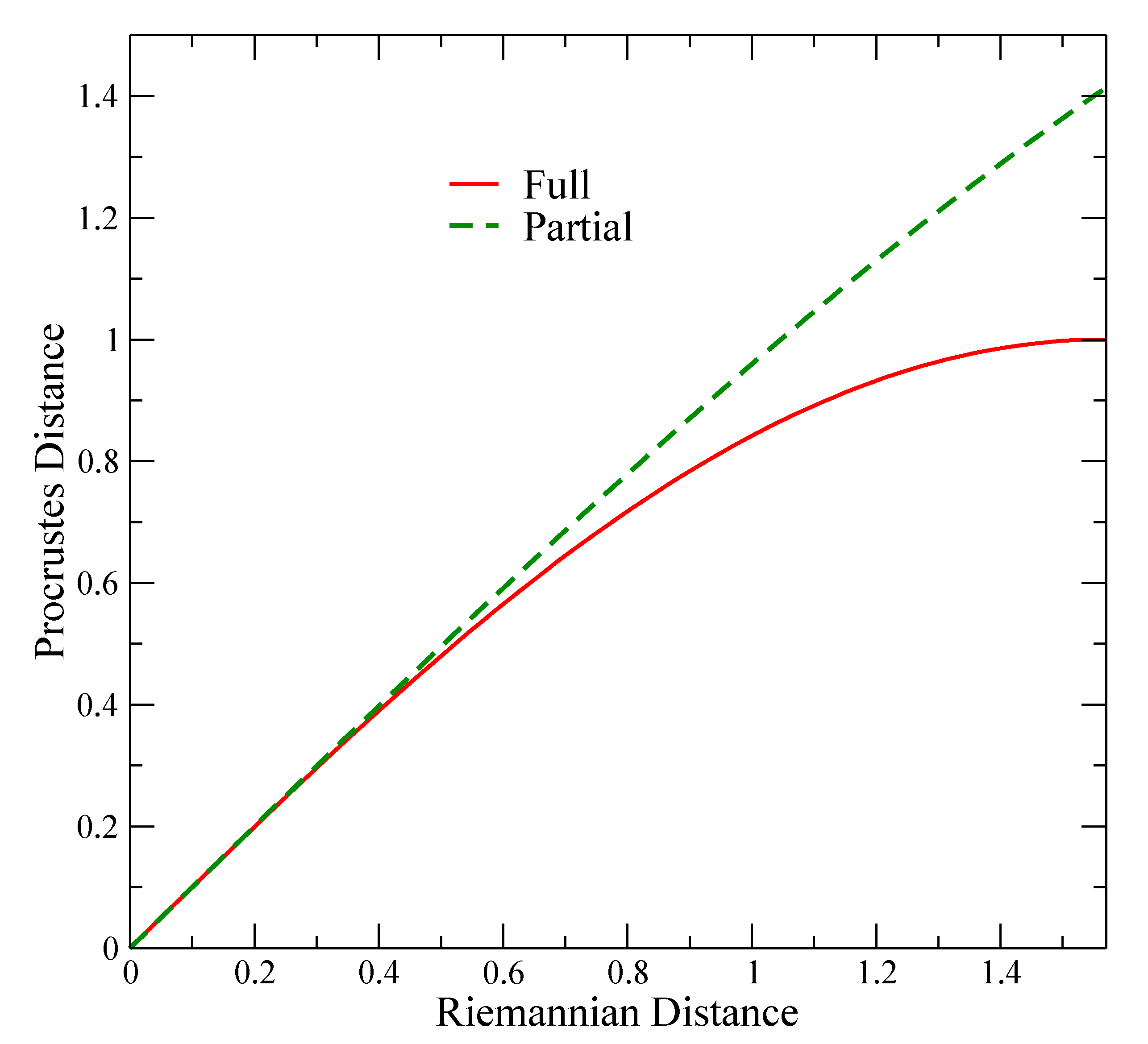
Thus, the validation with reference data (LANDSAT) of BA products are summarized in angles which can be order for establishing hierarchies of the products. Meanwhile, the full Procrustes distance is the Sine of the Riemannian distance; the partial Procrustes distance is the duplication of the sine of the half Riemannian distance. As shown in Figure 3, the trigonometrical relation between distances the full (Equation (3)) and partial Procrustes (Equation (4)) respect to the Riemannian distance are very similar for small angles (<0.90 approximately). It means that they behave similarly in presence of BA products near to reference data. Our interest pursues the same conclusion about the best product using the three distances. When the products are very different from reference data, the Riemannian, full, and partial Procrustes distances are near to , 1 or respectively, and this case is not of interest because the randomness of the measure exceeds the expertise of the product.
SM Section S3 shows a verification of the addressed properties by a simulation of the perturbation model. It shows the behavior of the three distances around the referred Properties 1 and 2 described in Section 2.3.1. Several simulations of the perturbation model were implemented in order to clarify each property.
2.3.3. Proposed Methods Based on Distances of Matrices
Following SM Section S3, we could continue with a number of simulations by changing the distributions in , and checking the behavior of the Riemannian, full, and partial Procrustes distances , but we do not know the true distributions of the perturbations. Instead, we use a method with the same power of simulations but considering resampling of the data that we really know. The bootstrap technique learns from the data and provides empirical distributions for the perturbations and the matrix distances as previously used in other contexts of remote sensing validation [40].
First Method: Comparison and Validation of BA Products by Bootstrap of Riemannian, Full or Partial Procrustes Distances
A simple comparison among the products is obtained by ordering the distances of all possible pairs of the five matrices related to each BA product: MCD64C6, MCD64C5, MCD45, Fire-CCI 4.1 (MERIS) and Fire-CCI 5.0 (MODIS). Then, we can establish similar or different performance according to the variables included in the columns. Now, a notorious discrepancy of two products can be explained from different sources. This can be attributed to dissimilarity in a few scenes or numerous scenes. One of the techniques refers to a more complex study of bootstrap exploring the distributions of the distances.
The method for validation works as follows:
- (1)
- Consider real BA products measure in the same scenes and variables of reference data. For each , we extract a sample with replacement of the scenes in the variables of interest and permute the rows of the product according that resample.
- (2)
- Let be the new resample product by rows.
- (3)
- Compute .
- (4)
- We repeat 1,000,000 times the above steps, then we obtain , and we can find the empirical probability density function of the Riemannian, Full or Partial Procrustes distances, under resampling of the rows. Then, inference and probability computations can be performed by using the real Riemannian or Procrustes distances .
The above method can also be used for comparison among the products. In this case we find empirical distributions for all the possible pairs of BA products .
The bootstrap method is carried out under resampling of the rows (scenes) allowing big differences (or similarities) without removing extreme data. If the discrepancy corresponds to few scenes, the resample tends to repeat equalities with similar performance, and there are more small differences than large ones. Thus, the distribution tends to be leptokurtic (unimodal, peaked, and narrow) and biased to the right, because the extremal differences are rare, then one can conclude that both BA products are statistically similar in most validation scenes, and a confidence interval of 95% and median estimation can be provided for the explanations and conclusions. Otherwise, when the discrepancy obeys several scenes, the bootstrap method tends to replace concordance scenes with extremely different performances and the distribution of the distance tends to be spread (platykurtic) and biased to the left. This indicates that both products are statistically different, and the addressed interval and median locations can support that conclusion. In the same way, it can explain the behavior of two products with a Riemannian, full, or partial Procrustes distances close to zero and the expected empirical distribution via bootstrap method. With the same philosophy, given that LANDSAT provides the reference data, a comparison with each BA product by using the bootstrap method reflects the statistical validation of the corresponding product according to the variables and scenes of interest. Certainly, the selection of well-defined variables, summarizing information of the local and proper characteristics of the BA, provides robust comparisons among the BA products and reference data validation. When a variable does not represent the field truth, the bootstrap method does not separate properly the corresponding performance. It is important to highlight that the bootstrap method is not constrained by Gaussian distributions, and is thus a robust statistical technique flexible to the distance distribution emerged from each pair under comparison or validation.
Second Method: Randomness and Permutation Tests for Validation of BA Products
The bootstrapping under zone resampling is a method for comparison and validation without deleting extreme discrepancies and similarity. Now, as a complementary analysis, one can focus on the implicit randomness of the measures by using a recent powerful statistical technique called permutation test [36]. The method explores the randomness in the measures of the BA products, in the scenes and ancillary variables under consideration. Namely, how much of the collected data of a BA product obeys the randomness than the expert theory behind the remote sensing technology.
The method is described as follows:
- (1)
- Consider a BA product and the usual reference data matrix .
- (2)
- Compute the true Riemannian, full, or partial distance .
- (3)
- Let the same matrix but with permuted rows according to certain permutation .
- (4)
- Compute .
- (5)
- Repeat times the steps (3) and (4). Then find the random Riemannian, Full or Partial Procrustes distances are obtained. Thus, the associated empirical probability density function of the Riemannian, full, or partial Procrustes distances are found.
- (6)
- Compute the probability that a random product reaches the true distance, i.e., .
- (7)
- Set the significant level of the permutation test as . If , then the permutation test rejects the hypothesis that the collected data by product are generated by randomness. Otherwise if the permutation test concludes that the data registered by are widely random and the true Riemannian, full, or partial Procrustes distances with can be obtained easily by a non expert technology.
- (8)
- Repeat the algorithm for all the products . The smallest p-value provides the “best” product according to the Property 1 of the Riemannian, full, or partial Procrustes distance described in the perturbation model of Section 2.3.1.
3. Results
3.1. Sample Size and Location of Sample Scenes
The application of SM Sections S1.1 and S1.2 provides 44 areas of validation on both continents: 17 in NHSA and 27 in NHAF. These scenes are marked by the black boxes in Figure 4a,b. The procedure and the results to calculate the sample size, provide identification of the validation scenes, and support the processing for the generation of the reference information can be found in SM Section S1.
3.2. First Method: Comparison and Validation of BA Products via Riemannian, Full and Partial Procrustes Distance Bootstraping
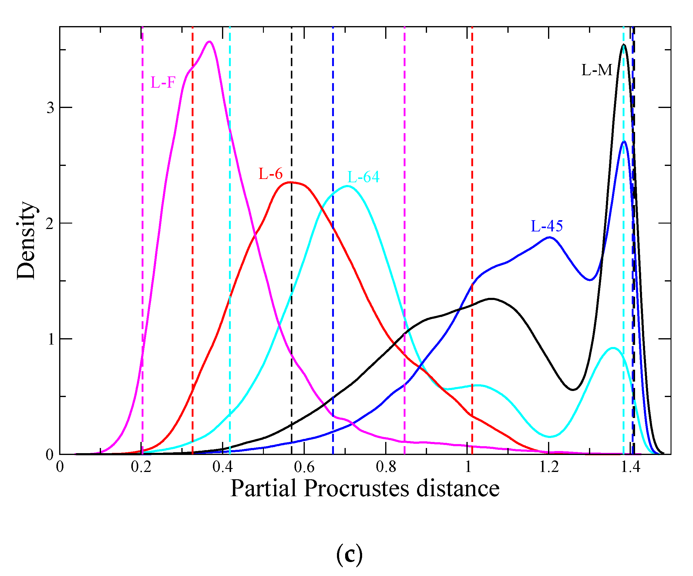
Now, we focus on the problem of comparison and validation of BA products by bootstrap of the Riemannian, full, and partial distances. Figure 5. Best global product using Bootstrap validation processes via matrix distances: (a) Riemannian, (b) Full Procrustes, (c) Partial Procrustes. The functions represent the smoothing of the frequency histogram of the three distances. In all cases, the magenta color (L-F) distribution ratifies that the Fire CCI 5.0 product is very near to the reference data (LANDSAT images). This distribution has a leptokurtic behavior, and the mean is also closer to the zero value. was obtained by applying the method of Section 2.3.3 (First Method). It reports the empirical probability density functions and 95% confidence intervals of the Riemannian distance bootstraping between the five pairs of validations BA products and reference data. In this case, we have considered the biomass sum, total BA, number of fires, P11, P12, P21, and P22 in the 44 scenes. Here, P11 is the proportion of BA according to both the product and the reference validation data (LANDSAT), P12 is the commission error area proportion, P21 is the omission error area proportion and P22 is the unburned area proportion according to both the product and the reference validation data (See SM Sections S2 and S2.1).
Each pair in the figure is shortly denoted, for example, L-F, corresponds to the density of all the Riemannian distances of reference data with the Fire-CCI 5.0 product under the 1,000,000 resampling experiment.
Note that similar validation conclusions of Riemannian distance (Figure 5a) are reached by using the full Procrustes distance (Figure 5b) and the partial Procrustes distance (Figure 5c).
These results suggest that the same method, based on Riemannian (Full or Partial Procrustes) distance bootstrapping, can be used for comparison and validation of several variables and subsets of the scenes. For example, we considered the validation and comparison of BA products with ecosystem variables, including biomass on each land cover, etc., and the most important results can be seen in SM Section S4 Table S4-1.
SM Section S4 Table S4-1 gives the results of 1050 simulations under several combinations of variables and regions. Each combination involves 10 pairs for comparison among the products and five pairs for validation with reference data. The selected variables include: Total BA, four components of error matrix, biomass sum, number of fires, fire size mean, three land cover types and two BIOME Olson types. Each simulation summarizes an intensive computational Riemannian distance bootstrapping of 100,000 resamples with replacement of the scenes. For space reasons, instead of providing the 1050 distribution functions as depicted in Figure 5. Best global product using Bootstrap validation processes via matrix distances: (a) Riemannian, (b) Full Procrustes, (c) Partial Procrustes. The functions represent the smoothing of the frequency histogram of the three distances. In all cases, the magenta color (L-F) distribution ratifies that the Fire CCI 5.0 product is very near to the reference data (LANDSAT images). This distribution has a leptokurtic behavior, and the mean is also closer to the zero value. a, we report the Riemannian distance mean of the corresponding empirical probability density function for each possible pair. The mean explains sufficiently the comparison of validation. A reported mean near to zero reflects equality for the pair because the distribution tends to be leptokurtic. Otherwise, a large mean is explained by highly platykurtic distribution due to strong differences in the leverage of the corresponding scenes of the pair. Note that the reported means for validation also define an order for the product performance. Similar computations for full and partial Procrutes distances were not included in the SM but they arrived at the same conclusions.
3.3. Second Method: Randomness and Permutation Tests for Validation of BA Products
In this section, we have applied the method of Section 2.3.3 (Second Method) for measuring the implicit randomness of the validation under different scenarios. Again, we present only the results about the Riemannian distance. The full and partial Procrustes distance gave similar results.
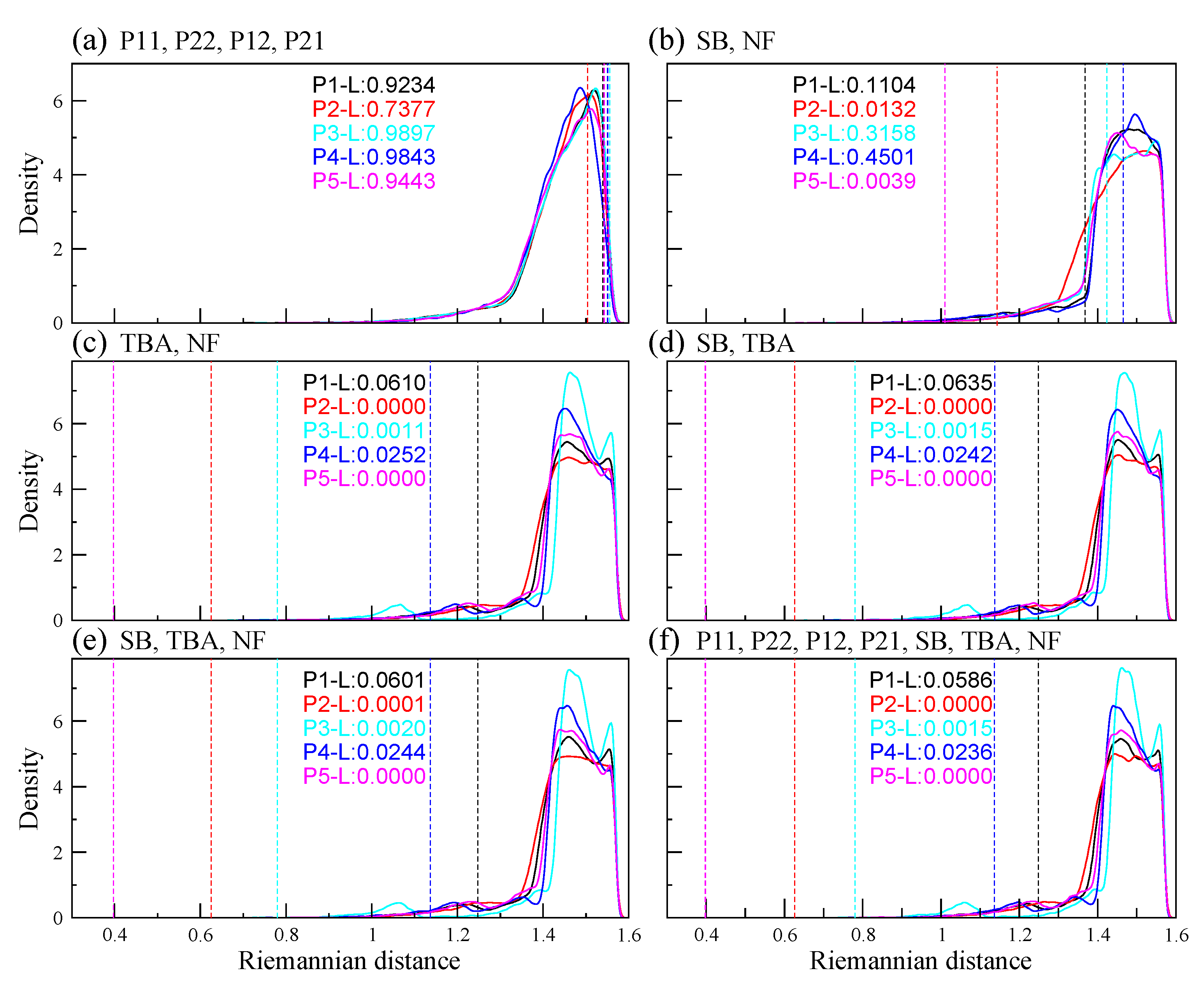
The Figure 6a–f depicts the empirical probability density function of the Riemannian distances associated to 100,000 random permutations of all the 44 scenes under study. Here. P1, P2, P3, P4, P5, and L stand for MCD64C5.1, MCD64C6, MCD45, Fire CCI 4.1, Fire CCI 5.0, and reference data. Also, we use the notation P11, P12, P21, and P22 for the elements of the error matrix. SB, TBA, and NF denote the sum of biomass, total BA, and number of fires, respectively. First, consider validation processes based on error matrices (Figure 6a). According to the discussion Figure 6a, the permutation tests fails for all the products, because the probability behind the observed true Riemannian distance with reference data is near to 1. However, once the sum of biomass and number of fires are considered, the permutation tests changes drastically by rejecting the null hypothesis. Then an order for the BA products can be established in terms of small p-values, see Figure 6b. Now, Figure 6c preserves a similar conclusion about the best two products, under the number of fires and total BA. When the sum of biomass and total BA are considered, both permutation tests of Figure 6c,d arrive at the same order for the BA products. Finally, Figure 6e shows the expected unified conclusion of Figure 6b–d for the three ancillary variables in the permutation tests. Note that the order, under a 0.0000 p-value and small distances, is preserved in the three referred combinations. The best product is Fire CCI 5.0, followed by MCD64C6. Observe that Figure 6f is consequent with Figure 6a,e. The inclusion of error matrix does not represent a significant improvement of the permutation tests under sum of biomass, total BA, and number of fires. The order of the performances preserved the conclusion of Figure 6e.
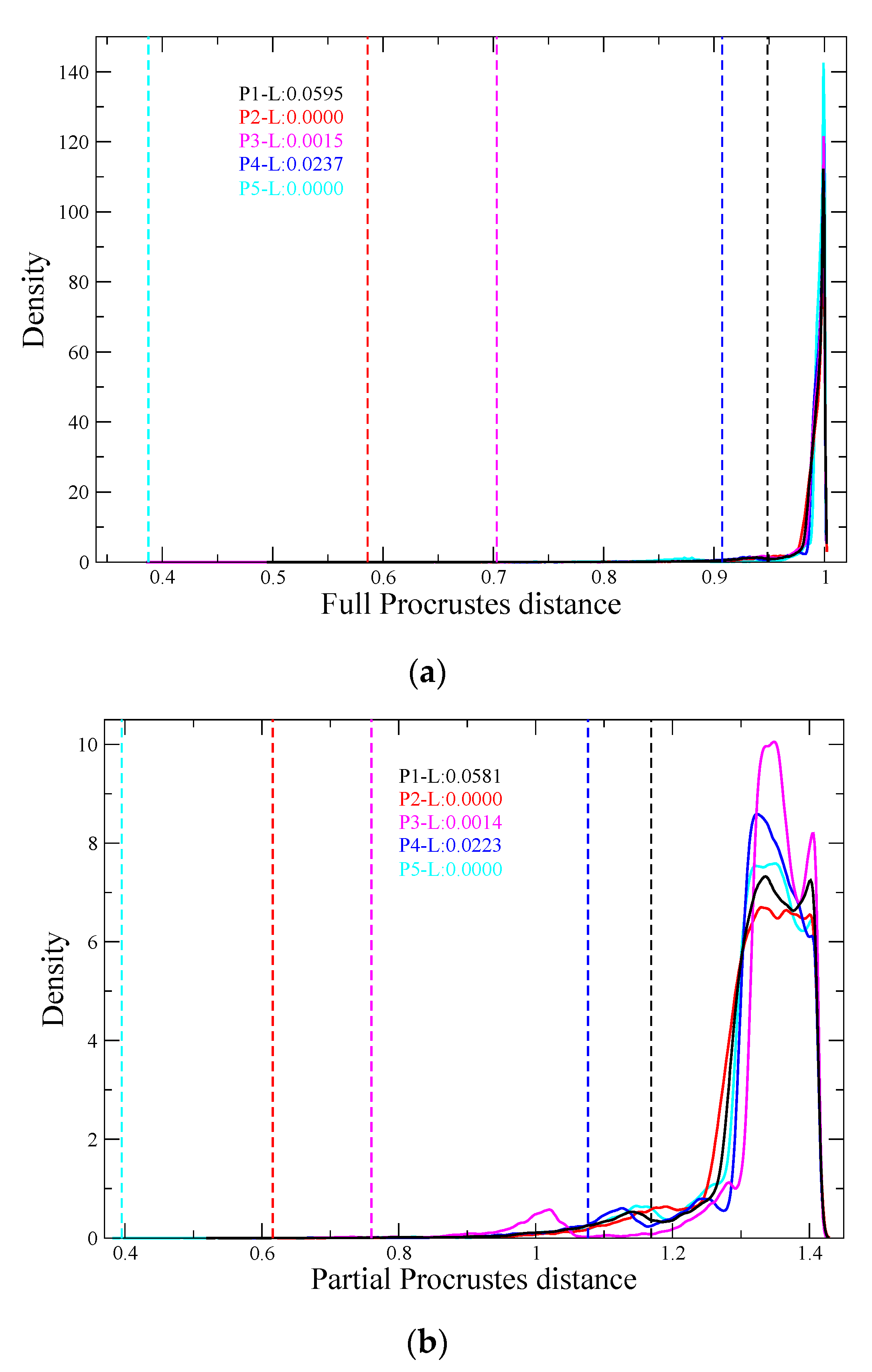
A similar conclusion to Figure 6e is obtained for the full Procrustes distance under the variables sum of biomass, total BA, and number of fires (see Figure 7a). Figure 7b shows a similar behavior of the permutation test of partial Procrustes distance under the same variables.
The results about the full and partial Procrustes distances are very similar. We highlight the best representative tests in Figure 6e.
The validation analysis is complemented with several permutation tests under different variables and continents. In order to include morphological and ecosystem information of the fires, we will focus on SB, TBA, and NF, but we will present the error matrix (P11, P22, P21, P12), (SB, NF). and (TBA, NF) for correctness (see Table 3.).
Explicitly, Table 3 and SM Section S5 (Table S5-1) give 260 permutation tests for validation of BA products under several combinations of variables and regions. The combinations include: validation scenes, three ecosystem types, and two BIOME Olson type. Each cell of the table collects the p-value of the Riemannian distance permutation test associated with an intensive computational exercise of 100.000 permutations of the scenes of the product. The p-value reports the probability that a non-expert product ruled by uncertainty can reach the same precision of the observed value in the validation scenes. The statistics of each test is given by the observed Riemannian distance between the BA product and reference data.
Certainly, there are several combinations of variables and scenes that can be considering for permutation tests and the corresponding conclusions can promote a future work. SM Section S5 shows some of those combinations involving continent, ecosystem type and Olson’s biomes.
4. Discussion and Assessment of Findings
The results of the paper have verified that comparison of BA products and their validation with reference data depend strongly of the quality of sampling, processing of the reference images, fire morphology, ecosystem variables, and constraints of the statistical models. Each issue can promote a deep investigation. However, we tried to propose a method with new insights of each one.
4.1. Sample Size Simulation, Zone Allocation and Descriptive Statistic Validation
For completeness and relations with traditional analysis, the SM Sections S1, S1.1–S1.3, S2, and S2.1 provide a number of results about information processing, sample size, validation zone allocation, and descriptive statistics with error matrix.
In both continents, the selected sample size was in agreement with the expert recommendation of Boschetti et al. [16].
Descriptive statistics of the error matrices given in SM Section S2 show high omission and commission errors. Then, it is impossible to order the global performance of the products. Each analysis using that matrix is highly randomly explained. As the reader can check in Supplementary Figures S2-1, S2-2, S2-3, and S2-4 and Supplementary Tables S2-1–2-5, the global behavior of the statistics is ruled by high randomness. As we have discussed, they lack of any geographical, morphological and ecosystem information for validation. The proposed methods include those variables and allow a classification for the products.
We have also noted that the classical method for a 500-m resolution in BA products is validated with LANDSAT images of 30-m resolution. Then, a significant underestimation appeared in the descriptive statistics Bias and RelBias, because small burned areas are not included. Although the Fire CCI Collection 4.1 product has 300 m of spatial resolution, a quality inherited from the MERIS sensor, a significantly lower temporal resolution was found compared to the data from MODIS. Using MODIS, information about the earth surface and atmospheric conditions can be obtained 2 times per day and twice at night, if we consider the swath its Terra and Aqua platforms over the course of a day. This also influenced the results.
By relating statistics like Oe, Ce, and RelB with the amount of burned area (in terms of LANDSAT burned pixels or reference data), it can be seen that all products have a tendency towards omission, and also that, in areas with a lower number of burned pixels, the products tend to omit 100% of the area that is actually burned.
The results obtained using traditional statistics indicated that high values for product accuracy when employing the global overall accuracy (OA) statistic are accompanied by little variability between the products analyzed. This reflects problems with the OA metric, as no one product is more representative than another. It can be observed that, in areas with few burnt pixels, all of the models used here are affected by the precision of the “unburned” class which causes an overestimation of the overall accuracy. Similar overvaluation using OA has been reported by References [2,6,30,60].
4.2. First Method: Comparison and Validation of BA Products via Riemannian, Full and Partial Procrustes Distance Bootstraping
The first contribution gives an alternative method for comparison of BA products and validation with reference data (LANDSAT images) by a stochastic modeling of the leverage of the scenes in each pair of interest. We have noted that storing the information of BA products and reference in a matrix can retain the dependency between the scenes and variables with respect to the Riemannian, full, or partial Procrustes distances. Given that the Riemannian distance is an angle (ranged from 0° to 90°) in a hypersphere then we can define an order for the validation of the BA products. The Full and Partial Procrustes distances have also a simple interpretation because they are similar with the Riemannian distance for BA products near to reference data. In that case, the products are not governed by randomness and all the conclusions are unified. When a product is very far from the reference data, the three distances are large and the comparison among then is not of interest. The distances were sensitive to changes in the matrix entries. In the simulations and the empirical distributions with real data, we have noted strong discrepancies and similarities of products with reference data, but it depended on the variables and continent, such that a useful order could be obtained for each case. The spatial analysis in the matrix distance setting showed a certain advantage over the use of the addressed descriptive statistics of bias, Relbias, OE, CE, AB, etc.
We have found also that ancillary variables have improved statistically the validation procedure, (see Supplementary Table S4-1). The results for comparison between the products and validation with reference data show the performance of the proposed method under several variables.
In general, the validation techniques based on Riemannian distance bootstraping identified Fire CCI 5.0 as the most accurate product, according to the empirical probability density function and the 95% confidence interval of distances. The list continues with MCD64C6, MCD64C5.1, MCD45 and Fire-CCI 4.1, Figure 5. Best global product using Bootstrap validation processes via matrix distances: (a) Riemannian, (b) Full Procrustes, (c) Partial Procrustes. The functions represent the smoothing of the frequency histogram of the three distances. In all cases, the magenta color (L-F) distribution ratifies that the Fire CCI 5.0 product is very near to the reference data (LANDSAT images). This distribution has a leptokurtic behavior, and the mean is also closer to the zero value, and SM (Supplementary Table S4-1 and S5-1). Note that the results for the validation of the BA products allow several classifications according to their performance by continents and ancillary variables. For example, in terms of the new variable total BA, the validation process refers to Fire CCI 5.0. The order continues with MCD64C6, MCD64C5.1, MCD45, and Fire CCI 4.1, (see Supplementary Table S4-1). However, if it is included the error matrix variables, all the products differ strongly from the reference values. Under the error matrix variables, if an order is required, despite the strong differences with reference data, the shape theory quotes that MCD45 is the nearest product to reference in NHSA. Then, the order follows with Fire-CCI 4.1, MCD64C6, MCD64C5.1, and Fire CCI 5.0. In NHAF, the selected variables maintain the discrepancies with reference data, but the order changes as follows: Fire CCI 5.0, MCD45, MCD64C5.1, MCD64C6, and Fire CCI 4.1 (see Supplementary Table S4-1).
If a new variable is incorporated, such as burned biomass, the Riemannian distance probability density function of Fire CCI 5.0 and reference data gets more leptokurtic, the mean tends to zero, and 95% confidence intervals are narrow. Meanwhile, the distribution of the remaining pairs tends to be more spread, multimodal, and platykurtic. If an order is required the list continues with: MCD64C6, MCD64C5.1, MCD45 and Fire CCI 4.1 (Supplementary Table S4-1). The same analysis by continent shows the following decreasing performance in NHSA: Fire CCI 5.0, MCD64C6, MCD64C5.1, Fire CCI 4.1, and MCD45 (see Supplementary Table S4-1). In NHAF, the results of the validation asses statistically that Fire CCI 5.0 is the nearest product of reference data. In fact, the remaining products are far from Fire CCI 5.0; the results propose the following decreasing order: Fire CCI 4.1, MCD64C6, MCD64C5.1, and MCD45 (see Supplementary Table S4-1).
The results agree with the technology behind Fire CCI 5.0 and the remaining BA products. When a product with different spatial resolution (250, 300, or 500 m) is validated with the reference, the spatial and thematic quality of the product influence the statistical results. In this case, BA product with less positional and thematic accuracy, incorporates more uncertainty.
The use of the shape theory also allowed for the inclusion of land cover variables and their relationship with the burned areas. It can be check that the cover in savannas was well detected by the five validated products, but Fire CCI 5.0 received the major statistical significance, followed by MCD64C6 (see SM S4 Table S4-1). Similarly, soils with crops mixed variables had a similar behavior for validation in NHAF. In fact, Fire CCI 5.0 and MCD products head the list of performance validation, but the results usually moved Fire CCI 4.1 Collection to the end. For the detection and quantification of fires in perennial forests, the statistical methods ratify the same conclusion: Fire CCI 5.0 is followed by similar MCD products and Fire CCI 4.1 is placed at the end. However, the statistical results in some scenes and variables give a wide gap when they are compared strictly with reference data.
The statistical methods also included validation of BA products under ecosystem variables. The results address a major statistical significance for Fire CCI 5.0 in savannas of NHSA; the remaining products share a similar detection resolution. Several validation scenes included the ecosystem type Sahela Acacia Savanna, the validation process provided a similar statistical significance to all the BA products. However, in the West Savanna ecosystem, the product Fire CCI 5.0 reached the main statistical significance, followed by both collections of MCD64; and according to the Riemannian distance bootstrapping the data collected by products MCD45 and Fire CCI 4.1 where located at the end of the statistical classification (see Supplementary Table S4-1).
Once the number of burned fragments is included in the validation, the collections of Fire CCI receives the main statistical significance in NHSA and NHAF. Similarly, if the burned biomass, then Fire CCI 5.0 resembles the reference data with the major statistical significance. Supplementary Table S4-1 also considers a combination of cover type variables with biomass, then the statistical results increase the significance for the BA products classification. Each one of the 1050 simulations enrich the analysis for comparison or validation and opens a future research.
When the Riemannian distance was replaced by Partial and Full Procrustes distances, the results were similar, then a robust conclusion about validation and comparison can be supported.
4.3. Second Method: Permutation Tests and Implicit Randomness of the Products in the Validation Process
We focused only in the validation process, but the technique can also be applied in comparison of products. The approach concerned the quantification of the randomness in the validation process. The permutation test of the Riemannian, full, or partial Procrustes distance of each pair product reference data suggested a measure of the randomness in the validation process under several combinations of variables and regions. It is based on the fact that a matching of expert data of a BA product with reference cannot be explained by uncertainty. It is a measure of the quality of the product and it is resistant to the usual Gaussian constraint. This second contribution of our study also provided several combinations of ecosystem variables with number of fires (related with fire morphology). It opens a perspective for validation beyond the general descriptive statistics of the proportions given in the error matrices.
The work also derived dozens of results which can be used for future validation routines. The addressed bootstrap with resampling of scenes and permutation tests for random explanation, consolidate two complementary methods for the validation of a BA product with reference data.
We highlight that 57 of the 65 permutation tests based on error matrices variables do not reject the null hypothesis of random explanation of the reference. Table 3 and Supplementary Table S5-1 show that the observed Riemannian distance (the value in parenthesis) between the BA product and reference data is large; then an arbitrary permutation of the scenes in the product can reach easily the same distance with the reference, and then the p-value of the test is high. Only a few pairs in ecosystem Sahelian Acacia Savanna rejected the null hypothesis with a 5% level.
However, if we use ancillary variables SB, TBA, NF, most of the permutation tests gives at least a product with low p-value (observed Riemannian distance near to zero) and a statistically significant order of the products can be given. For example, Fire CCI 5.0 resembled the reference data with a statistically significant level of 5% in most of the combinations. MCD64C6 was the second product with a meaningful statistical performance. When all the ecosystem and Biome Olson variables are included, the permutation tests of Table 3 provide a statistical significance for at least one product. Only the validation of products under the Sahelian Acacia Savanna ecosystem in NHAF cannot reject the corresponding null hypothesis.
Permutations test are useful for suggesting meaningful variables. If we consider the number of fires and total BA, the Riemannian distances of the products are closer to reference data (see Figure 6c). If we remove the strong randomness of P11, P22, P12, and P21 the differences among the products became clear and are agree with the results of the previous section based on bootstrapping) Figure 6b–f). The same results were obtained with the full and partial Procrustes distances, as shown in Figure 7a,b.
Finally, a few combinations in Table 3 and Supplementary Table S5-1 provide problems for the validation of all the products. Thus, a research concerning the detection of some ecosystem and Biome Olson types will open interesting perspectives in future.
We highlight that the results given in Section 3.2 and Section 3.3 agree with simulations of the perturbation model given in SM Section S3.
5. Conclusions
This work proposed two methods for validation-comparison of BA products: (1) a Riemannian, full and partial Procrustes distance distribution bootstrapping was used for the comparison of BA products and their validation with reference data, and (2) a second technique for the validation of BA products was studied under Riemannian, full, and partial Procrustes distance permutation tests. The description of the Riemannian, full, and partial Procrustes distance was also examined under controlled simulations, and the real data verified the behavior under perturbations and row resample of the reference data matrix.
Each part of the method studied the literature context of the existing techniques. Part 1 studied the empirical probability density function of Riemannian, full, and partial distance of the matrices indexed by the validation scenes and new ancillary variables. Then, part 2 considered the implicit randomness of the products under permutation of the validation scenes. A list of hierarchies for BA products was obtained by the three distances under several combinations of ancillary variables, continents, land cover, and biome Olson type.
Error matrix and associated descriptive statistics are based on general proportions of omission, commission, agreement and disagreement. These proportions cannot describe the morphological, ancillary and location variables. They offer a local validation that hardly defines the best product when there are different validation scenes with morphological variables and wide ecosystems. Additionally, they do not include the spatial location of the validation scenes, eliminating the statistical richness provided by georeferenced systems. When the proportions of the error matrix are included together with the ancillary variables in our method, the proportions lose weight in the comparison-validation because the new descriptors are georeferenced and describe the morphological truth and the particular ecosystem.
Our methods suggested the inclusion of the scene location, the number of fires by pixel and several ancillary variables such as biomass, ecosystem type and biome Olson type. Parts (1) and (2) summarized the data in matrices collecting the scenes and variables, then the products and reference are compared by using three different distances. The distances behave equally under BA products near to the reference. When the products are far from the reference, the distances are large, and the randomness rules their performance and explanation of the truth. Part 1 measured the leverage of the validation scenes by studying the empirical probability density function of a bootstrap for the Riemannian, Full and Partial Procrustes distances. Then, the best product emerged from unimodal, peaked, and narrow distributions and an order for the performance can be proposed. Further, part 2 explored the validation under arbitrary permutations of the validation scenes with the same distances. A test for implicit randomness of the products can be performed. Then, a p-value near to zero refers a BA product with the best performance under the studied variables. Hundreds of intensive computational simulations were performed under several regions, ancillary variables, and distances. Both methods suggested that Fire CCI 5.0 has the major statistical significance under several combinations of ecosystem, biomass, BA, and number of fires. MCD64C6 led the statistical significance in some experiments. In general, all the computations have collected multiple similarities and differences of the BA products that can be explored in a future research.
Moreover, new insights involving the dynamics and connexity of fires will be part of a subsequent work.
The methods for validation and comparison here derived and those mentioned in the Supplementary Material can be used in other contexts of remote sensing, such as the accuracy assessment of land cover products and quality validation of cartographic products.
Supplementary Materials
The following are available online at https://www.mdpi.com/2072-4292/12/23/3972/s1, from S1 to S5, Figure S1-1. (a) Distribution for the commission errors in a pilot experiment in order to model the sample size and errors for validation scenes in NHSA. (b) Implemented method based on a pilot experiment and optimization of Equation (1a). The optimal Equations (1b) and (1c) are used to define 17 validations scenes in NHSA with associated error of 22%. A similar procedure suggests a sample size of 27 scenes for NHAF, Figure S1-2. Distribution of active fires from the Fire Information for Resource Management System (FIRMS) [8].Study area NHSA. December 2015, Figure S1-3: Validation zones in the Andean region of the NHSA. a) Validation zones generated from the BAMS model. b) Validation zones generated from the BAMS model and including cloud mask and cloud shadows of the LEDAPS model. 7/4/3 RGB color cannon (LANDSAT 7) March 2007, Figure S2-1. Omission and commission of BA products. Green squares at zero RelB% correspond to the reference area. The points represent the statistics of each validation zone. The RelB statistic of a product gives the tendency to omission (−) or commission (+), Figure S2-2. Patterns of omission and commission for each BA product. The size of each point represents the coincident BA (m2) between the BA product and the reference. The points represent the statistics of each validation zone. The square in green shows the reference with commission/omission error free. Observe the extreme concentration of errors above the 50%, Figure S2-3. Comparison between omission and commission by continent. The points represent the statistics of each validation zone. Note again the high concentration of errors above the 50%., Figure S2-4. Representativeness of validated products according to the type of ecosystem. Ecosystem type reference information extracted from the Olson biomes. This graph shows the amount of total BA in km2 detected by each of the validated products and their reference (LANDSAT). Note that in the NHSA the ecosystem “Llanos” is the most affected by burning. While in the NHAF the most affected ecosystem was “Northern Congolian forest savanna mosaic “, Figure S3-1. Simulated Riemannian distance of 93 products perturbed from matrix L from a sample of 10.000 non-central t-distribution of 2 degrees of freedom and non centrality parameter of 3% to 93%. (a) Property (1) of Riemannian distance, red, black and green symbols corresponds to minimum, maximum and median values. (b) Property (2) of Riemannian distance, Figure S3-2. Simulated Full Procrustes Distance of 93 products perturbed from matrix L from a sample of 10.000 non central t distribution of 2 degrees of freedom and non centrality parameter of 3% to 93%. (a) Property (1) of Full Procrustes Distance, red, black and green symbols corresponds to minimum, maximum and median values. (b) Property (2) of Full Procrustes Distance, Figure S3-3. Simulated Partial Procrustes distance of 93 products perturbed from matrix L from a sample of 10.000 non-central t-distribution of 2 degrees of freedom and non centrality parameter of 3% to 93%. (a) Property (1) of Partial Procrustes Distance, red, black and green symbols corresponds to minimum, maximum and median values. (b) Property (2) of Partial Procrustes Distance, Table S2-1. Descriptive statistics of error matrices for Fire CCI 4.1, Table S2-2. Descriptive statistics of error matrices for MCD45C5.1, Table S2-3. Descriptive statistics of error matrices for MCD64C5.1, Table S2-4. Descriptive statistics of error matrices for MCD64C6.0, Table S2-5. Descriptive statistics of error matrices for Fire CCI 5.0 Product, Table S4-1. Riemannian distance comparison per variable in each validation zone, Table S5-1. Permutation test and Riemannian distance comparison per variable in each validation zone.
Author Contributions
Conceptualization, G.M.V., F.J.C.-L., and J.A.A.; data curation, G.M.V., F.J.C.-L., and R.R.; Formal analysis, G.M.V., F.J.C.-L., J.A.A., and É.A.V.; Funding acquisition, G.M.V.; Investigation, G.M.V., F.J.C.-L., and R.R.; Methodology, G.M.V., and F.J.C.-L.; Writing—original draft, G.M.V.; Writing—review & editing, F.J.C.-L., J.A.A., and É.A.V. All authors have read and agreed to the published version of the manuscript.
Funding
This research was funded by Universidad de San Buenaventura-Colombia, Colciencias-Colombia Doctoral Scholarship Program 567, code PDBCNAL 71331711, and Universidad de Medellín-Colombia.
Acknowledgments
The authors wish to acknowledge the contributions of the MODIS, MERIS, Fire CCI, FIRMS, and LANDSAT programs. They are also grateful to Universidad de San Buenaventura-Medellín through its postgraduate program specializing in Geographic Information Systems and its MSc in Geoinformatics, the Universidad de Medellín through his PhD in Engineering and PhD in Modeling and Scientific Computing, and the University of Alcalá through his PhD in Geographic Information Technologies and its Laboratory of Environmental Remote Sensing. We also thank Colciencias- Colombia project for its significant support to the training of PhD research, Doctoral Scholarship Program 567. Finally, we want to give special thanks to Emilio Chuvieco for his support, inspiration and accompaniment, during the doctoral internship of the researcher Germán Valencia.
Conflicts of Interest
The authors declare no conflict of interest.
References
- Van Der Werf, G.R.; Randerson, J.T.; Giglio, L.; Collatz, G.J.; Mu, M.; Kasibhatla, P.; Morton, D.C.; DeFries, R.S.; Jin, Y.; Van Leeuwen, T.T. Global fire emissions and the contribution of deforestation, savanna, forest, agricultural, and peat fires (1997–2009). Atmos. Chem. Phys. Discuss. 2010, 10, 11707–11735. [Google Scholar] [CrossRef] [Green Version]
- Padilla-Parellada, M.; Stehman, S.; Ramo, R.; Corti, D.; Hantson, S.; Oliva, P.; Alonso-Canas, I.; Bradley, A.V.; Tansey, K.; Mota, B.W.; et al. Comparing the accuracies of remote sensing global burned area products using stratified random sampling and estimation. Remote. Sens. Environ. 2015, 160, 114–121. [Google Scholar] [CrossRef] [Green Version]
- Giglio, L.; Randerson, J.T.; Van Der Werf, G.R. Analysis of daily, monthly, and annual burned area using the fourth-generation global fire emissions database (GFED4). J. Geophys. Res. Biogeosci. 2013, 118, 317–328. [Google Scholar] [CrossRef] [Green Version]
- Giglio, L.; Boschetti, L.; Roy, D.P.; Humber, M.L.; Justice, C. The Collection 6 MODIS burned area mapping algorithm and product. Remote Sens. Environ. 2018, 217, 72–85. [Google Scholar] [CrossRef] [PubMed]
- Anaya-Acevedo, J.A.; Colditz, R.R.; Valencia, G.M. Land Cover Mapping of a Tropical Region by Integrating Multi-Year Data into an Annual Time Series. Remote Sens. 2015, 7, 16274–16292. [Google Scholar] [CrossRef] [Green Version]
- Randerson, J.T.; Chen, Y.; Van Der Werf, G.R.; Rogers, B.M.; Morton, D.C. Global burned area and biomass burning emissions from small fires. J. Geophys. Res. Space Phys. 2012, 117. [Google Scholar] [CrossRef]
- Juárez-Orozco, S.M.; Siebe, C.; Fernández, D.F.Y. Causes and Effects of Forest Fires in Tropical Rainforests: A Bibliometric Approach. Trop. Conserv. Sci. 2017, 10. [Google Scholar] [CrossRef]
- Giglio, L.; Randerson, J.T.; Van Der Werf, G.R.; Kasibhatla, P.; Collatz, G.J.; Morton, D.C.; DeFries, R.S. Assessing variability and long-term trends in burned area by merging multiple satellite fire products. Biogeosciences 2010, 7, 1171–1186. [Google Scholar] [CrossRef] [Green Version]
- Chuvieco, E.; Lizundia-Loiola, J.; Pettinari, M.L.; Ramo, R.; Padilla, M.; Tansey, K.; Mouillot, F.; Laurent, P.; Storm, T.; Heil, A.; et al. Generation and analysis of a new global burned area product based on MODIS 250 m reflectance bands and thermal anomalies. Earth Syst. Sci. Data 2018, 10, 2015–2031. [Google Scholar] [CrossRef] [Green Version]
- Avitabile, V.; Herold, M.; Heuvelink, G.B.M.; Lewis, S.L.; Phillips, O.L.; Asner, G.P.; Armston, J.D.; Ashton, P.S.; Banin, L.; Bayol, N.; et al. An integrated pan-tropical biomass map using multiple reference datasets. Glob. Chang. Boil. 2016, 22, 1406–1420. [Google Scholar] [CrossRef] [Green Version]
- Hu, T.; Su, Y.; Xue, B.; Liu, J.; Zhao, X.; Fang, J.; Guo, Q. Mapping Global Forest Aboveground Biomass with Spaceborne LiDAR, Optical Imagery, and Forest Inventory Data. Remote Sens. 2016, 8, 565. [Google Scholar] [CrossRef] [Green Version]
- Rodríguez-Veiga, P.; Wheeler, J.; Louis, V.; Tansey, K.; Balzter, H. Quantifying Forest Biomass Carbon Stocks From Space. Curr. Rep. 2017, 3, 1–18. [Google Scholar] [CrossRef] [Green Version]
- Van Der Werf, G.R.; Randerson, J.T.; Giglio, L.; Van Leeuwen, T.T.; Chen, Y.; Rogers, B.M.; Marle, M.; Morton, M.J.E.; Collatz, D.C.; James, G.; et al. Global fire emissions estimates during 1997–2016. Earth Syst. Sci. Data 2017, 9, 697–720. [Google Scholar] [CrossRef] [Green Version]
- Van Marle, M.; Kloster, S.; Magi, B.I.; Marlon, J.; Daniau, A.-L.; Field, R.D.; Arneth, A.; Forrest, M.; Hantson, S.; Kehrwald, N.M.; et al. Historic global biomass burning emissions for CMIP6 (BB4CMIP) based on merging satellite observations with proxies and fire models (1750–2015). Geosci. Model. Dev. 2017, 10, 3329–3357. [Google Scholar] [CrossRef] [Green Version]
- Padilla, M.; Stehman, S.V.; Chuvieco, E. Validation of the 2008 MODIS-MCD45 global burned area product using stratified random sampling. Remote Sens. Environ. 2014, 144, 187–196. [Google Scholar] [CrossRef]
- Boschetti, L.; Stehman, S.V.; Roy, D.P. A stratified random sampling design in space and time for regional to global scale burned area product validation. Remote Sens. Environ. 2016, 186, 465–478. [Google Scholar] [CrossRef]
- Armenteras, D.; Gibbes, C.; Anaya-Acevedo, J.A.; Dávalos, L.M. Integrating remotely sensed fires for predicting deforestation for REDD+. Ecol. Appl. 2017, 27, 1294–1304. [Google Scholar] [CrossRef]
- Andela, N.; Van Der Werf, G.R.; Kaiser, J.W.; Van Leeuwen, T.T.; Wooster, M.J.; Lehmann, C. Biomass burning fuel consumption dynamics in the tropics and subtropics assessed from satellite. Biogeosciences 2016, 13, 3717–3734. [Google Scholar] [CrossRef] [Green Version]
- Santana, L.D.; Ribeiro, J.H.C.; Berg, E.V.D.; Carvalho, F.A. Impact on soil and tree community of a threatened subtropical phytophysiognomy after a forest fire. Folia Geobot. Et Phytotaxon. 2020. [Google Scholar] [CrossRef]
- Chu, T.; Guo, X. Remote Sensing Techniques in Monitoring Post-Fire Effects and Patterns of Forest Recovery in Boreal Forest Regions: A Review. Remote Sens. 2013, 6, 470–520. [Google Scholar] [CrossRef] [Green Version]
- Palomino, S.; Anaya, J.A. Evaluation of the Causes of Error in the Mcd45 Burned-Area Product for the Savannas of Northern South America. Dyna Colomb. 2012, 79, 35–44. [Google Scholar]
- Roy, D.; Boschetti, L.; Justice, C.O.; Ju, J. The collection 5 MODIS burned area product—Global evaluation by comparison with the MODIS active fire product. Remote Sens. Environ. 2008, 112, 3690–3707. [Google Scholar] [CrossRef]
- Congalton, R.G.; Green, K. Assessing the Accuracy of Remotely Sensed Data: Principles and Practices, 2nd ed.; Lewis Publishers: Sound Parkway-Boca Raton, FL, USA, 2009. [Google Scholar]
- Boschetti, L.; Roy, D.P.; Justice, C.O. CEOS International Global Burned Area Satellite Product Validation Protocol, Part I—Production and Standardization of Validation Reference Data. 2010. Available online: https://lpvs.gsfc.nasa.gov/PDF/BurnedAreaValidationProtocol.pdf (accessed on 7 March 2019).
- Schepers, L.; Haest, B.; Veraverbeke, S.; Spanhove, T.; Borre, J.V.; Goossens, R. Burned Area Detection and Burn Severity Assessment of a Heathland Fire in Belgium Using Airborne Imaging Spectroscopy (APEX). Remote Sens. 2014, 6, 1803–1826. [Google Scholar] [CrossRef] [Green Version]
- Nogueira, J.; Ruffault, J.; Chuvieco, E.; Mouillot, F. Can We Go Beyond Burned Area in the Assessment of Global Remote Sensing Products with Fire Patch Metrics? Remote Sens. 2016, 9, 7. [Google Scholar] [CrossRef] [Green Version]
- Singh, G. A Multi-Sensor Approach For. Burned Area Extraction Due to Crop. Residue Burning Using Multi-Temporal Satellite Data. Degre of Master of Science in Geo-information Science and Earth Observation, ITC Netherlands and IIRS India. 2008. Available online: http://www.iirs.gov.in/iirs/sites/default/files/StudentThesis/gurdeep.pdf (accessed on 21 May 2019).
- Long, T.; Zhang, Z.; He, G.; Jiao, W.; Tang, C.; Wu, B.; Zhang, X.; Wang, G.; Yin, R. 30 m Resolution Global Annual Burned Area Mapping Based on Landsat Images and Google Earth Engine. Remote Sens. 2019, 11, 489. [Google Scholar] [CrossRef] [Green Version]
- Roy, D.P.; Frost, P.G.H.; Justice, C.O.; Landmann, T.; Le Roux, J.L.; Gumbo, K.; Makungwa, S.; Dunham, K.; Du Toit, R.; Mhwandagara, K.; et al. The Southern Africa Fire Network (SAFNet) regional burned-area product-validation protocol. Int. J. Remote Sens. 2005, 26, 4265–4292. [Google Scholar] [CrossRef]
- Roy, D.; Boschetti, L. Southern Africa Validation of the MODIS, L3JRC, and GlobCarbon Burned-Area Products. IEEE Trans. Geosci. Remote Sens. 2009, 47, 1032–1044. [Google Scholar] [CrossRef]
- De Santis, A.; Chuvieco, E.; Vaughan, P.J. Short-term assessment of burn severity using the inversion of PROSPECT and GeoSail models. Remote Sens. Environ. 2009, 113, 126–136. [Google Scholar] [CrossRef]
- Negri, J.A. Evaluation and Validation of Multiple Predictive Models Applied to Post-Wildfire Debris-Flow Hazards. Degree of Master of Science (Geological Engineering), Colorado School of Mines. 2016. Available online: https://mountainscholar.org/handle/11124/170086?show=full (accessed on 8 August 2020).
- Ghasemi, A.; Zahediasl, S. Normality Tests for Statistical Analysis: A Guide for Non-Statisticians. Int. J. Endocrinol. Metab. 2012, 10, 486–489. [Google Scholar] [CrossRef] [Green Version]
- Limpert, E.; Stahel, W.A. Problems with Using the Normal Distribution—And Ways to Improve Quality and Efficiency of Data Analysis. PLoS ONE 2011, 6, e21403. [Google Scholar] [CrossRef] [Green Version]
- Stahl, S. Evolution of the Normal Distribution. In Mathematics Magazine; Taylor & Francis: Beloit, WI, USA, 2014; pp. 96–113. [Google Scholar]
- Faraway, J.J. Linear Models with R; Texts in Statistical Science Series; Chapman & Hall/CRC: Boca Raton, FL, USA, 2005. [Google Scholar]
- Roteta, E.; Bastarrika, A.; Padilla, M.; Storm, T.; Chuvieco, E. Development of a Sentinel-2 burned area algorithm: Generation of a small fire database for sub-Saharan Africa. Remote Sens. Environ. 2019, 222, 1–17. [Google Scholar] [CrossRef]
- Roy, D.P.; Huang, H.; Boschetti, L.; Giglio, L.; Yan, L.; Zhang, H.K.; Li, Z. Landsat-8 and Sentinel-2 burned area mapping—A combined sensor multi-temporal change detection approach. Remote Sens. Environ. 2019, 231, 111254. [Google Scholar] [CrossRef]
- Boschetti, L.; Roy, D.P.; Giglio, L.; Huang, H.; Zubkova, M.; Humber, M.L. Global validation of the collection 6 MODIS burned area product. Remote Sens. Environ. 2019, 235, 111490. [Google Scholar] [CrossRef] [PubMed]
- Valencia, G.M.; Anaya-Acevedo, J.A.; Caro-Lopera, F.J. Implementación y evaluación del modelo Landsat Ecosystem Disturbance Adaptive Processing System (LEDAPS): Estudio de caso en los Andes colombianos. Rev. Teledetección 2016, 46, 83. [Google Scholar] [CrossRef] [Green Version]
- Cook, J.R.; Stefanski, L.A. Simulation-Extrapolation Estimation in Parametric Simulation-Extrapolation Estimation in Parametric Measurement Error Models. J. Am. Stat. Assoc. 1994, 89, 1314–1328. [Google Scholar] [CrossRef]
- Giglio, L.; Csiszar, I.; Justice, C.O. Global distribution and seasonality of active fires as observed with the Terra and Aqua Moderate Resolution Imaging Spectroradiometer (MODIS) sensors. J. Geophys. Res. Space Phys. 2006, 111, 1–12. [Google Scholar] [CrossRef]
- Alvarado, S.T.; Fornazari, T.; Costola, A.; Morellato, L.P.C.; Silva, T. Drivers of fire occurrence in a mountainous Brazilian cerrado savanna: Tracking long-term fire regimes using remote sensing. Ecol. Indic. 2017, 78, 270–281. [Google Scholar] [CrossRef] [Green Version]
- Alvarado, S.T.; Silva, T.; Archibald, S.A. Management impacts on fire occurrence: A comparison of fire regimes of African and South American tropical savannas in different protected areas. J. Environ. Manag. 2018, 218, 79–87. [Google Scholar] [CrossRef] [Green Version]
- Dong, X.; Fu, J.S.; Huang, K.; Lin, N.-H.; Wang, S.-H.; Yang, C.-E. Analysis of the Co-existence of Long-range Transport Biomass Burning and Dust in the Subtropical West Pacific Region. Sci. Rep. 2018, 8, 8962. [Google Scholar] [CrossRef] [Green Version]
- Hurteau, M.D.; Liang, S.; Westerling, A.L.; Wiedinmyer, C. Vegetation-fire feedback reduces projected area burned under climate change. Sci. Rep. 2019, 9, 2838. [Google Scholar] [CrossRef] [Green Version]
- Kettridge, N.; Lukenbach, M.; Hokanson, K.; Hopkinson, C.; Devito, K.; Petrone, R.; Mendoza, C.; Waddington, J.M. Extreme wildfire exposes remnant peat carbon stocks to increased post-fire drying. In Proceedings of the 20th EGU General Assembly Conference Abstracts EGU2018, Vienna, Austria, 4–13 April 2018; Volume 20, p. 8399. [Google Scholar]
- Mouillot, F.; Schultz, M.G.; Yue, C.; Cadule, P.; Tansey, K.; Ciais, P.; Chuvieco, E. Ten years of global burned area products from spaceborne remote sensing—A review: Analysis of user needs and recommendations for future developments. Int. J. Appl. Earth Obs. Geoinf. 2014, 26, 64–79. [Google Scholar] [CrossRef] [Green Version]
- Giglio, L.; Van Der Werf, G.R.; Randerson, J.T.; Collatz, G.J.; Kasibhatla, P. Global estimation of burned area using MODIS active fire observations. Atmos. Chem. Phys. Discuss. 2005, 5, 11091–11141. [Google Scholar] [CrossRef] [Green Version]
- Bastarrika, A.; Alvarado, M.; Artano, K.; Martínez, M.P.; Mesanza-Moraza, A.; Torre-Tojal, L.; Ramo, R.; Chuvieco, E. BAMS: A Tool for Supervised Burned Area Mapping Using Landsat Data. Remote Sens. 2014, 6, 12360–12380. [Google Scholar] [CrossRef] [Green Version]
- Masek, J.G.; Vermote, E.F.; Saleous, N.E.; Wolfe, R.; Hall, F.G.; Huemmrich, K.F.; Gao, F.; Kutler, J.; Lim, T.K. A Landsat Surface Reflectance Dataset for North America, 1990–2000. IEEE Geosci. Remote Sens. Lett. 2006, 3, 68–72. [Google Scholar] [CrossRef]
- Claverie, M.; Vermote, E.; Franch, B.; Masek, J.G. Evaluation of the Landsat-5 TM and Landsat-7 ETM+ surface reflectance products. Remote Sens. Environ. 2015, 169, 390–403. [Google Scholar] [CrossRef]
- Chuvieco, E.; Yue, C.; Heil, A.; Mouillot, F.; Alonso-Canas, I.; Padilla, M.; Pereira, J.M.C.; Oom, D.; Tansey, K. A new global burned area product for climate assessment of fire impacts. Glob. Ecol. Biogeogr. 2016, 25, 619–629. [Google Scholar] [CrossRef] [Green Version]
- Olson, D.M.; Dinerstein, E.; Wikramanayake, E.D.; Burgess, N.D.; Powell, G.V.; Underwood, E.C.; D’amico, J.A.; Itoua, I.; Strand, H.E.; Morrison, J.C.; et al. Terrestrial Ecoregions of the World: A New Map of Life on Earth. Bioscience 2001, 51, 933–938. [Google Scholar] [CrossRef]
- ESA. Land Cover CCI Product User Guide Version 2. Tech. Rep. 2017. Available online: http://maps.elie.ucl.ac.be/CCI/viewer/download/ESACCI-LC-Ph2-PUGv2_2.0.pdf (accessed on 8 August 2020).
- Dryden, I.L.; Mardia, K.V. Statistical Shape Analysis, with Applications in R.; Wiley: Chichester, West Sussex, UK, 2016. [Google Scholar]
- Quintero, J.H.; Mariño, A.; Šiller, L.; Restrepo-Parra, E.; Caro-Lopera, F. Rocking curves of gold nitride species prepared by arc pulsed—Physical assisted plasma vapor deposition. Surf. Coat. Technol. 2017, 309, 249–257. [Google Scholar] [CrossRef]
- Arias, E.; Caro-Lopera, F.J.; Florez, E.; Pérez-Torres, J.F. Two Novel Approaches Based on the Thompson Theory and Shape Analysis for Determination of Equilibrium Structures of Nanoclusters: Cu8, Ag8 and Ag18 as study cases. J. Phys. Conf. Ser. 2019, 1247, 012008. [Google Scholar] [CrossRef]
- Villarreal-Rios, A.L.; Calle, A.H.B.; Caro-Lopera, F.J.; Ortiz-Méndez, U.; García-Méndez, M.; Pérez-Ramírez, F.O. Ultrathin tunable conducting oxide films for near-IR applications: An introduction to spectroscopy shape theory. SN Appl. Sci. 2019, 1, 1553. [Google Scholar] [CrossRef] [Green Version]
- Boschetti, L.; Roy, D.P.; Justice, C.; Humber, M.L. MODIS–Landsat fusion for large area 30m burned area mapping. Remote Sens. Environ. 2015, 161, 27–42. [Google Scholar] [CrossRef]
Figure 1.
Different fire morphologies can provide the same error matrix. Reports of products with (a) area burned of - fires- of 1 pixel, versus—(b) A single fire- of pixels, or (c) separated fires that sum pixels.
Figure 1.
Different fire morphologies can provide the same error matrix. Reports of products with (a) area burned of - fires- of 1 pixel, versus—(b) A single fire- of pixels, or (c) separated fires that sum pixels.

Figure 2.
Map of the 14 GFED regions. Regions defined in studies of L. Giglio et al., (2006, 2010) [8,42,49].

Figure 3.
Relation between the Riemannian distance and the Procrustes distances (Full and Partial). The three distances behave similar in presence of BA products close to reference data (LANDSAT).
Figure 3.
Relation between the Riemannian distance and the Procrustes distances (Full and Partial). The three distances behave similar in presence of BA products close to reference data (LANDSAT).

Figure 4.
Study area, 44 Validation scenes are shown as black rectangles that correspond to the extent of a LANDSAT image. (a) NHSA, (b) NHAF. The different land cover types art shown in a map from the CCI-LC project of (ESA) http://maps.elie.ucl.ac.be/CCI/viewer/.
Figure 4.
Study area, 44 Validation scenes are shown as black rectangles that correspond to the extent of a LANDSAT image. (a) NHSA, (b) NHAF. The different land cover types art shown in a map from the CCI-LC project of (ESA) http://maps.elie.ucl.ac.be/CCI/viewer/.

Figure 5.
Best global product using Bootstrap validation processes via matrix distances: (a) Riemannian, (b) Full Procrustes, (c) Partial Procrustes. The functions represent the smoothing of the frequency histogram of the three distances. In all cases, the magenta color (L-F) distribution ratifies that the Fire CCI 5.0 product is very near to the reference data (LANDSAT images). This distribution has a leptokurtic behavior, and the mean is also closer to the zero value. The validation performances of the remaining products, under the three distances, are easily identified by the locus of the mean value and the confidence limits. Here L-6, L-64, L-45 and L-M, stand for the validation of MCD64C6, MCD64C5.1, MCD45 and Fire CCI 4.1, respectively. The last two products show a platykurtic behavior, with high tendency to dissimilarity (big biased to pi/2).


Figure 6.
Behavior of the permutation test applying bootstrap simulation and Riemannian distances on different validation variables. (a) elements of the error matrix P11, P22, P12 and P21. (b) sum of biomass and number of fires. (c) number of fires and total BA. (d) sum of biomass and total BA. (e) sum of biomass, total BA, and number of fires. (f) all the elements of the error matrix: P11, P22, P12 and P21, sum of biomass, total BA, and number of fires. Here P1, P2, P3, P4, P5 and L stand for MCD64C5.1, MCD64C6, MCD45, Fire CCI 4.1, Fire CCI 5.0 and reference data.

Figure 7.
Randomness and permutation tests for validation of BA products via Procrustes distances. (a) Permutation test for Full Procrustes Distance and the variables P11, P22, P12, P21, sum of biomass, total BA, and number of fires. (b) Permutation test for Partial Procrustes Distance under the variables P11, P22, P12, P21, sum of biomass, total BA, and number of fires.


Table 1.
List of BA products analyzed in this study.
| Product Name | Sensor | Reference | Source |
|---|---|---|---|
| MCD45A1 Collection 5.1 | Generated from MODIS 500m images | MCD45 [22] | University of Maryland |
| MCD64A1 Collection 5.1 | Generated from MODIS 500 m Collection 5 images, and information about thermal anomalies in the same sensor | MCD64C5.1 [3] | University of Maryland |
| MCD64A1 Collection 6 | Generated from MODIS 500 m Collection 6 images, and information about thermal anomalies in the same sensor plus information from the VIIRS sensor | MCD64C6 [4] | University of Maryland |
| Fire CCI 4.1 | Generated from Envisat-MERIS 300 m images, and thermal anomaly information detected with the MODIS sensor | Fire CCI 4.1 [53] | University of Alcalá, CCI program |
| Fire CCI 5.0 | Generated from the Red and NIR bands of the MODIS 250 m sensor, and information about thermal anomalies detected with the MODIS sensor, | Fire CCI 5.0 [9] | University of Alcalá, CCI program |
Table 2.
Ancillary variables considered in the global analysis.
| Variable | Product | Observation |
|---|---|---|
| Land cover | CCI Global Land Cover [55] | Download site: https://www.esa-landcover-cci.org/ |
| Biomass | Pan-tropical map of aboveground woody biomass [10] | Download site: https://www.wur.nl/en/Research-Results/Chair-groups/Environmental-Sciences/Laboratory-of-Geo-information-Science-and-Remote-Sensing/Research/Integrated-land-monitoring/Forest_Biomass.htm |
| Ecoregions | Terrestrial Ecoregions of the World (TEW) [54] | Download site: https://www.worldwildlife.org/publications/terrestrial-ecoregions-of-the-world |
| Number of burned fragments (LANDSAT) | Validation Polygons generated from LANDSAT image processing | |
| Total BA LANDSAT | Total BA obtained from LANDSAT image processing |
Table 3.
p-values of permutation test for validation under different scenarios and variables. The statistic of the test is the true Riemannian distance (in parenthesis) between the product and reference matrices. Note that the true Riemannian distances near to zero are associated with p-values close to zero. Rejecting the permutation test with such small p-value means that a random generator cannot obtain the same observed values for the product. The opposite conclusion can be addressed when true Riemannian distance is very far from zero, then the permutation test, with a p value near to 1, cannot be rejected. It means that the data measured by the product can be easily obtained by a random generator, without any technological expertise. P-values of the table also serves for ordering the product respect the performance under the variables of interest. The tests also allow ordering among statistical significant groups of variables.
| Variables | Scenes | Type of Ecosystem | BIOME Olson | P1-L | P2-L | P3-L | P4-L | P5-L |
|---|---|---|---|---|---|---|---|---|
| Error matrix | NHSA-NHAF | All | All | 0.9276 (1.540) | 0.7360 (1.504) | 0.9905 (1.556) | 0.9867 (1.551) | 0.9461 (1.542) |
| SB, TBA, NF | All | All | All | 0.0575 (1.248) | 0.0000 (0.626) | 0.0018 (0.780) | 0.0216 (1.137) | 0.0000 (0.398) |
| SB, NF | All | All | All | 0.1047 (1.367) | 0.0117 (1.143) | 0.3124 (1.423) | 0.4619 (1.465) | 0.0042 (1.009) |
| TBA, NF | All | All | All | 0.0586 (1.248) | 0.0000 (0.626) | 0.0019 (0.780) | 0.0231 (1.137) | 0.0000 (0.398) |
| Error matrix | NHSA | All | All | 0.9116 (1.506) | 0.7468 (1.457) | 0.8439 (1.486) | 0.8119 (1.480) | 0.9486 (1.523) |
| SB, TBA, NF | NHSA | All | All | 0.0270 (0.961) | 0.0000 (0.349) | 0.0007 (0.643) | 0.0693 (0.929) | 0.0000 (0.258) |
| SB, NF | NHSA | All | All | 0.7069 (1.454) | 0.1841 (1.234) | 0.8775 (1.484) | 0.6093 (1.426) | 0.0425 (1.070) |
| TBA, NF | NHSA | All | All | 0.0306 (0.961) | 0.0000 (0.348) | 0.0008 (0.643) | 0.0739 (0.929) | 0.0000 (0.258) |
| Error matrix | NHAF | All | All | 0.8602 (1.519) | 0.8597 (1.511) | 0.8196 (1.511) | 0.9318 (1.516) | 0.5723 (1.444) |
| TBA, NF | NHAF | All | All | 0.0464 (1.128) | 0.0420 (1.071) | 0.0552 (1.219) | 0.0171 (0.967) | 0.0273 (1.022) |
| SB, TBA, NF | NHAF | All | All | 0.0433 (1.128) | 0.0397 (1.071) | 0.0541 (1.219) | 0.0158 (0.967) | 0.0278 (1.022) |
| SB, NF | NHAF | All | All | 0.0011 (0.664) | 0.0000 (0.599) | 0.2868 (1.435) | 0.0001 (0.445) | 0.0013 (0.382) |
Publisher’s Note: MDPI stays neutral with regard to jurisdictional claims in published maps and institutional affiliations. |
© 2020 by the authors. Licensee MDPI, Basel, Switzerland. This article is an open access article distributed under the terms and conditions of the Creative Commons Attribution (CC BY) license (http://creativecommons.org/licenses/by/4.0/).
Share and Cite
MDPI and ACS Style
Valencia, G.M.; Anaya, J.A.; Velásquez, É.A.; Ramo, R.; Caro-Lopera, F.J. About Validation-Comparison of Burned Area Products. Remote Sens. 2020, 12, 3972. https://doi.org/10.3390/rs12233972
AMA Style
Valencia GM, Anaya JA, Velásquez ÉA, Ramo R, Caro-Lopera FJ. About Validation-Comparison of Burned Area Products. Remote Sensing. 2020; 12(23):3972. https://doi.org/10.3390/rs12233972
Chicago/Turabian StyleValencia, Germán M., Jesús A. Anaya, Éver A. Velásquez, Rubén Ramo, and Francisco J. Caro-Lopera. 2020. "About Validation-Comparison of Burned Area Products" Remote Sensing 12, no. 23: 3972. https://doi.org/10.3390/rs12233972
Note that from the first issue of 2016, this journal uses article numbers instead of page numbers. See further details here.