Article

An Assessment of the Hydrological Trends Using Synergistic Approaches of Remote Sensing and Model Evaluations over Global Arid and Semi-Arid Regions

1
Schmid College of Science and Technology, Chapman University, Orange, CA 92866, USA
2
Center of Excellence in Earth Systems Modeling and Observations, Chapman University, CA 92866, USA
3
Department of Environmental Sciences, Faculty of Science, Alexandria University, Moharem Bek, Alexandria 21522, Egypt
4
Computational and Data Sciences Graduate Program, Schmid College of Science and Technology, Chapman University, Orange, CA 92866, USA
5
Center for Environment and Water, The Research Institute, King Fahd University of Petroleum & Minerals (KFUPM), Dhahran 31261, Saudi Arabia
*
Author to whom correspondence should be addressed.
Remote Sens. 2020, 12(23), 3973; https://doi.org/10.3390/rs12233973
Submission received: 10 November 2020 / Revised: 30 November 2020 / Accepted: 2 December 2020 / Published: 4 December 2020
(This article belongs to the Special Issue Advances of Remote Sensing in Mapping Arid/Semi-arid Environment)

Abstract

:
Drylands cover about 40% of the world’s land area and support two billion people, most of them living in developing countries that are at risk due to land degradation. Over the last few decades, there has been warming, with an escalation of drought and rapid population growth. This will further intensify the risk of desertification, which will seriously affect the local ecological environment, food security and people’s lives. The goal of this research is to analyze the hydrological and land cover characteristics and variability over global arid and semi-arid regions over the last decade (2010–2019) using an integrative approach of remotely sensed and physical process-based numerical modeling (e.g., Global Land Data Assimilation System (GLDAS) and Famine Early Warning Systems Network (FEWS NET) Land Data Assimilation System (FLDAS) models) data. Interaction between hydrological and ecological indicators including precipitation, evapotranspiration, surface soil moisture and vegetation indices are presented in the global four types of arid and semi-arid areas. The trends followed by precipitation, evapotranspiration and surface soil moisture over the decade are also mapped using harmonic analysis. This study also shows that some hotspots in these global drylands, which exhibit different processes of land cover change, demonstrate strong coherency with noted groundwater variations. Various types of statistical measures are computed using the satellite and model derived values over global arid and semi-arid regions. Comparisons between satellite- (NASA-USDA Surface Soil Moisture and MODIS Evapotranspiration data) and model (FLDAS and GLDAS)-derived values over arid regions (BSh, BSk, BWh and BWk) have shown the over and underestimation with low accuracy. Moreover, general consistency is apparent in most of the regions between GLDAS and FLDAS model, while a strong discrepancy is also observed in some regions, especially appearing in the Nile Basin downstream hyper-arid region. Data-driven modelling approaches are thus used to enhance the models’ performance in this region, which shows improved results in multiple statistical measures ((RMSE), bias ( ψ ), the mean absolute percentage difference ( | ψ | ) ) and the linear regression coefficients (i.e., slope, intercept, and coefficient of determination (R2)).

Graphical Abstract

1. Introduction

Arid and semi-arid regions, also known as drylands, are areas where the annual total surface evaporation and vegetation transpiration substantially exceeds precipitation. Recent studies show that they account for about 40% of the Earth’s land surface [1] and play an important role in the process of global climate change as a regulator of trends and variabilities of atmospheric carbon dioxide (CO2) concentrations [2,3,4,5]. Anders et al. [2] showed that the mean sink, trend, and interannual variability in CO2 uptake by terrestrial ecosystems are influenced by diverse biogeographic regions where the trend and interannual variability of the sink are largely influenced by semi-arid ecosystems. In fact, Joel et al. [3] suggested that the contribution of the dryland regions towards the changing regional and global CO2 exchange may be three to five times larger than current estimates. Benjamin et al. [5] found that the global carbon cycle inter-annual variability is driven by the carbon pools in semi-arid biomes. Due to the lack of water supplies, low vegetation coverage, and fragile ecological environment in these areas, these regions are suitable for activities with lower annual productivity and more sensitive and rapid in response to external forces. In the past 100 years, the arid and semi-arid regions have been the areas with the most significant land temperature increase and area expansion [6,7]. The situation is projected to intensify, as indicated by climate models [8,9], likely resulting in an increase in aridity, warming, along with land degradation and desertification in the drylands of developing countries [7]. The drylands would also undergo the consequences of climate change through emissions from humid lands [7,10].
Nowadays, more than two billion people live in these regions, with about 90% of them from developing countries where people’s living standards and technological capabilities lag far behind developed countries [1]. The interaction of anthropogenic activities (e.g., farming, grazing and irrigation) and natural processes is suggested to have a strong influence on the water balance. The increasing demand for water resources in support of these activities can exacerbate the severity of existing drought conditions. Mitigation actions such as groundwater exploitation for irrigation and industry would alleviate the ongoing situation yet increase the vulnerability for upcoming droughts. Therefore, moderate to severe droughts, combined with the depletion of surface and groundwater resources, pose significant risks to water and food security, leading to wide-ranging and long-term impacts, including conflicts among dryland countries over shared transboundary river basins. As a result, there is a pressing need to improve our understanding of the ongoing situations and the future trends of hydrological parameters in these global arid and semi-arid regions to perform proper mitigation assessments for these important and vulnerable ecosystems.
Dryland vegetation is strongly governed by the spatial and temporal variation of water availability. These variables show apparent links between hydrology and ecology in these regions, where the temporal variation of precipitation is more substantial than other areas at different scales (diurnal, seasonal and interannual). Generally, precipitation pulses trigger a cascade of pulsed ecosystem responses to end dry periods. Meanwhile, they can also lead to a rapid increase in evapotranspiration (ET), which consists mainly of evaporation (E) from plant and soil surfaces and plant transpiration (T) through leaf stomata. Consequently, transpiration can contribute significantly to total ET if the water added is adequate to wet the root zone, indicated by the surface/sub-surface soil moistures [3,11,12,13,14]. In drylands, ET is an effective indicator of vegetation resilience and resistance to drought conditions, since water is the major constraint on plant productivity [15,16]. In the hydrological cycle, ET also serves as a key process that links energy, carbon and water cycles [17].
Ground-based observation networks, mainly from eddy covariance flux towers, have been established to estimate various variables such as ET and gross primary productivity (GPP). Some typical networks include FLUXNET [18], AmeriFlux [19], ILTER [20] and NEON [21]. These sites are mostly situated in more humid and developed areas, while large drylands in Africa, South America, Middle East, and central Asia have limited representation. Remote sensing has been functional in demonstrating the role of GPP and ET, as well as ecosystem structure within the context of the broader Earth system [4,5]. Favorable atmospheric conditions (lower cloud coverage) in drylands offer advantages for optical remote sensing and increase the chances of high-quality observations. In addition, pioneering technologies were developed in drylands, including the retrieval of surface reflectance [22,23], as well as quantitative estimates of vegetation conditions and photosynthetic capacity in the rangelands of the Great Plains [24]. The later research afterward became the Normalized Difference Vegetation Index (NDVI) [25], calculated as NDVI = (NIR − R)/(NIR + R), which is generally based on the high reflectivity of plants in the near-infrared (NIR) wavelength range and the high absorption by plants in the red (R) wavelength range for photosynthesis. With spectral normalization, NDVI minimizes effects from topographic variation, sun-sensor geometry and shadows [26], thus becoming one of the most widely used vegetation indices [26,27,28]. The long-term and high-frequency NDVI time series retrievals, like the 23 year time series generated for long-term studies of the Sahel region [26], enhanced our understanding of the long-term trends and driving forces behind regional dryland dynamics. In Australia, an analysis to check whether vegetation cover increased was conducted using calibrated advanced very high-resolution radiometer data spanning 1981–2006 [27]. In the same region, an analysis of the decadal time-scale changes was conducted using AVHRR GIMMS NDVI dataset to check the relationship between a proxy for vegetation productivity and annual rainfall [28]. Subsequently, Randall et al. [29] observed a greening of the globe over recent decades which they attributed to CO2 fertilization effect. A study by Ramus et al. [30] to analyze trends in vegetation greenness of semi-arid areas showed an increase in greenness found both in semi-arid areas where precipitation is the dominating limiting factor for plant production and where air temperature is the primary growth constraint. Similarly, Ulf et al. [31] in their research using NOAA AVHRR data in Mediterranean basin, the Sahel from the Atlantic to the Red Sea, major parts of the drylands of Southern Africa, China–Mongolia and the drylands of South America showed a greening-up. Other studies conducted by Kolby et al. [32], which showed an increase in net primary productivity (NPP), and by Zaichun et al. [33], which discussed the greening of earth and its drivers, attributed the major cause to be CO2 fertilization. These investigations recently elucidated that global drylands greening is largely due to CO2 fertilization’s effects in the context of global climate change [29,30,31,32,33]. Since the 2000s, there has been an exponential increase in the volume of remote sensing data, resulting from newly launched sensors and products, as well as higher resolution domains (spatial, temporal, and spectral). Such expansion of big data revolutionized our understanding of the Earth system, while posing a higher request for advances in data management and processing capability. Accordingly, increasing the availability of cloud-based computing and analytical platforms, such as Amazon Web Service (AWS) and Google Earth Engine [34], is being widely used for dryland research [35,36,37,38,39,40]. Using the tools within Google Earth Engine, it was found that global dryland tree cover was significantly underrated and recent estimates exceeded previous ones by over 40% [41].
The goal of this paper is to evaluate hydrologic and land cover changes in global arid/semi-arid regions over the last decade (2010–2019), through time series and trends analysis, correlation and interactions of multiple hydrological indicators and vegetation indices. Another key point of this research is to evaluate two major process-based land surface modeling and data assimilation models (GLDAS and FLDAS) by satellite-based hydrological products. Additional analysis displayed an overestimation of surface soil moisture (SSM) and an underestimation of evapotranspiration (ET), as well as a discovery of a strong discrepancy observed in Egypt by the aforementioned models. To mitigate this discrepancy, machine learning models using extra data from satellites (Moderate Resolution Imaging Spectroradiometer (MODIS)) were developed which increased the process-based model performance significantly and provided results with lower RMSE and bias. This optimization effort highlights the promising applications of the synergistic approach of data-driven and process-based modeling for hydrological studies.
This paper is organized into four sections. The information regarding the study area, data sources and methods are described in Section 2. Section 3.1 illustrates the time series boxplots of multiple hydrological parameters used over arid regions. In Section 3.2, the trends of ET, soil moisture and precipitation during the period of 2010–2019 over global drylands are presented. Section 3.3 shows the landcover and water storage changes of selected areas. In Section 3.4, the comparison between FLDAS and GLDAS surface soil moisture and ET products is shown by correlation maps, followed by the approach of data-driven modelling of the aforementioned products. Finally, the results are discussed in detail in Section 4 and a conclusion in Section 5 is provided for the paper.

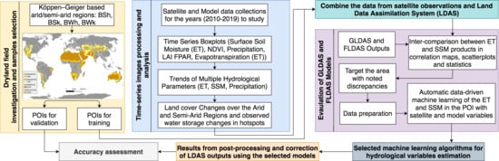
2. Materials and Methods
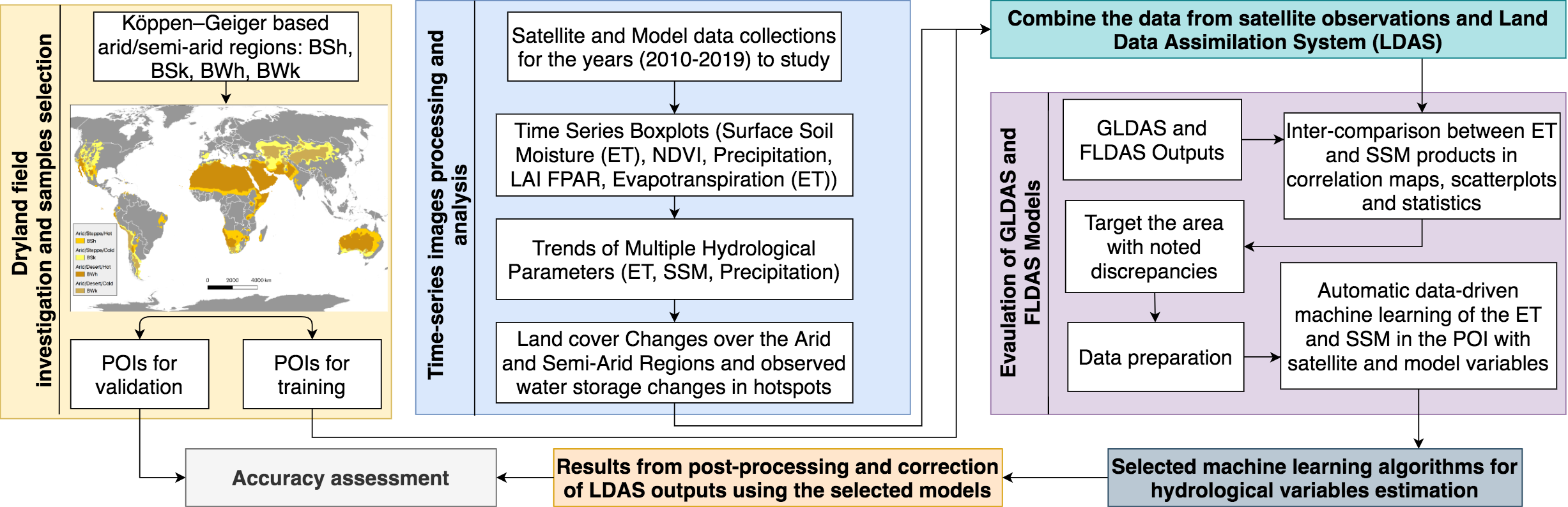
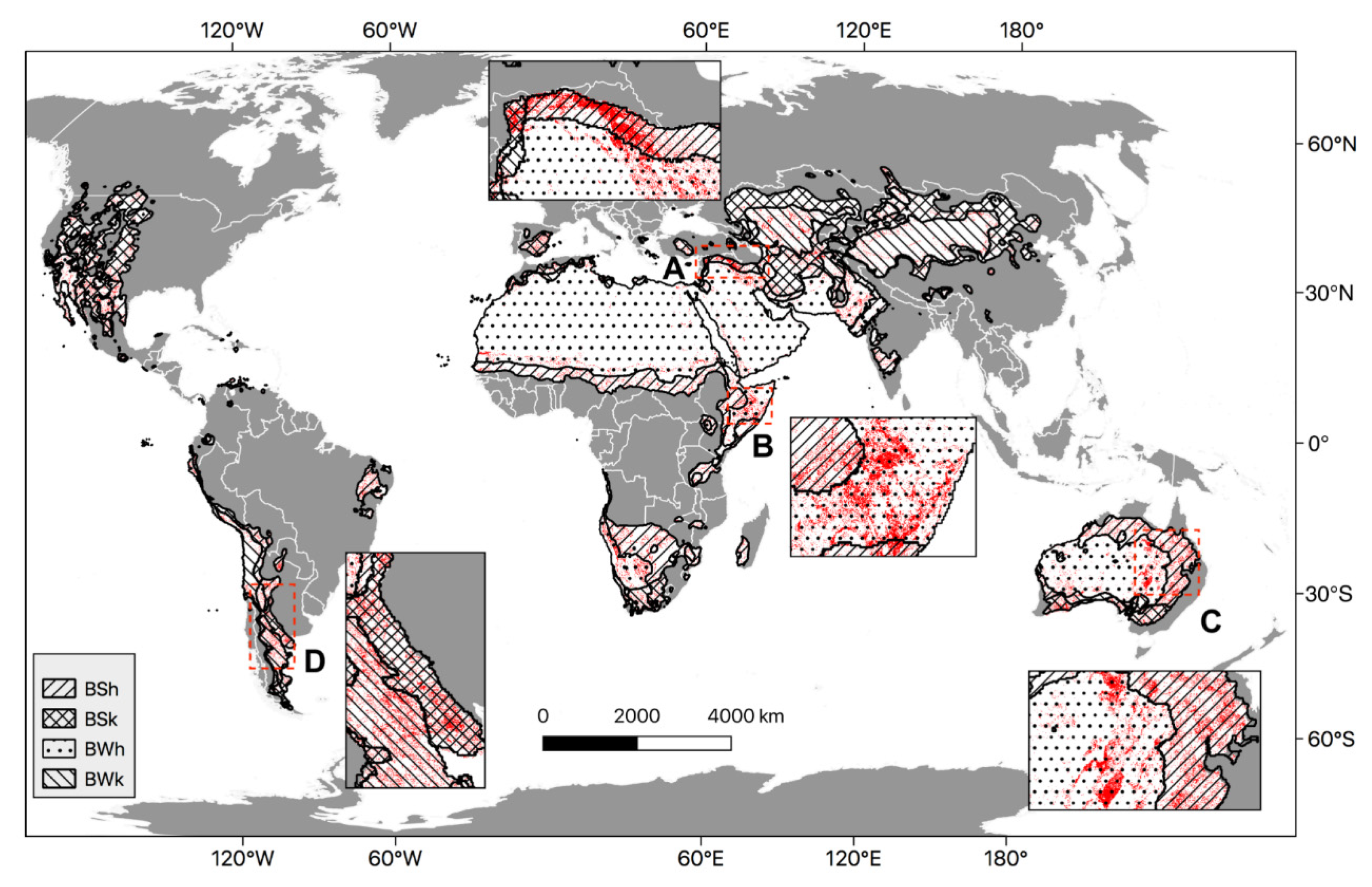
2.1. Study Area

The global arid and semi-arid regions were selected from the updated version of the Köppen–Geiger climate map [42], which shows five main climate groups, with sub-division of each group based on seasonal precipitation and temperature patterns. The five main groups are A (tropical), B (dry), C (temperate), D (continental), and E (polar). In this research, the subgroups starting with the letter “B” (dry) were identified as arid and semi-arid classes, namely, BWh (hot desert climates), BWk (cold desert climates), BSh (hot steppe climates) and BSk (cold steppe climates) (Figure 1a). The corresponding biome type distribution over these regions is also presented in Figure 1b using OpenLandMap Potential distribution of biomes dataset [43].

2.2. Data

2.2.1. Data from Remote Sensing Observations

  • Precipitation Data
The precipitation data used in this study were obtained from the Climate Hazards Group Infrared Precipitation with Station (CHIRPS) dataset (version 2.0) [44], with 0.05° spatial resolution satellite imagery, and were converted into monthly temporal resolution. Developed by Earth Resource Observation and Science Center and the United States Geological Survey (USGS), CHIRPS is a 30+ year quasi-global rainfall dataset incorporating satellite and station data and to create gridded precipitation time series for hydrology monitoring and correlational and trend studies.
  • Surface Soil Moisture Data
The surface soil moisture data were obtained from the National Aeronautics and Space Administration (NASA)–United States Department of Agriculture (USDA) Global Soil Moisture Dataset [45,46,47,48], with 0.25° spatial resolution and monthly temporal resolution. This dataset is generated through the data assimilation approach using a modified two-layer Palmer model using a 1-D ensemble Kalman filter (EnKF) to integrate the satellite-derived soil moisture observations. This dataset includes products of soil moisture profile (%), surface and subsurface soil moisture, as well as their standardized anomalies values computed using a 31 day moving window.
  • Water Storage Data
The changes in groundwater storage are represented by the variations in the water equivalent height (in cm) observed from the Gravity Recovery and Climate Experiment (GRACE) and GRACE Follow-on mission monthly gravitational anomalies datasets [49,50,51] in 1° spatial resolution. GRACE is a twin satellite setup that measures global changes in water anomalies. These anomalies depict the changes in the total water column represented by water equivalent height, which includes surface, sub-surface, and groundwater components.
  • Vegetation Indices Data
The Moderate Resolution Imaging Spectroradiometer (MODIS) sensor onboard of Terra satellite provides three vegetation index products: evapotranspiration (ET) [52], NDVI [53], Leaf Area Index (LAI) and fraction of absorbed photosynthetically active radiation (FPAR) [54]. All the products are regridded and converted into monthly data over 1 km spatial resolution. The calculation of MODIS ET is affected by other variables, including albedo, biomes type and LAI [52]. LAI is defined as half the total leaf area per unit ground area [55]. FPAR is defined as the fraction of the incoming solar radiation that is absorbed by a photosynthetic organism in the photosynthetically active radiation spectral region. The MODIS products are proved to effectively capture the dominant seasonal LAI and FPAR patterns in many arid and semi-arid ecosystems [56].

2.2.2. Data from Process-Based Models

The Land Data Assimilation Systems (LDAS) use data from multiple ground and space observations that are integrated with advanced numerical models of physical processes to simulate fields of water and energy states and fluxes, which helps in filling gaps and minimizing errors in the observations. Different projects (e.g., NLDAS, GLDAS, FLDAS) of LDAS have been configured for specific domains and purposes [57]. There are some known issues with GLDAS version 1 data, which might present some challenges in the runoff, soil moisture and ET analysis performed with the GLDAS model. These issues are suggested to be solved in the newer version (GLDAS version 2.1) used in this study. The GLDAS 2.1 simulation started on 1 January 2000 using the conditions from the GLDAS version 2.0 simulation. The GLDAS-2.1 is revised with upgraded models using National Oceanic and Atmospheric Administration (NOAA)/Global Data Assimilation System (GDAS) atmospheric analysis fields [58], the disaggregated Global Precipitation Climatology Project (GPCP) precipitation fields [59] and the Air Force Weather Agency’s AGRiculturalMETeorological modeling system (AGRMET) radiation fields. In this study, the surface soil moisture and evapotranspiration were selected from the GLDAS-2.1 Noah model from 2010 to 2019, with its 0.25 degree spatial resolution and monthly temporal resolution.
FLDAS [60] is designed for semi-arid, food-insecure regions of Africa. Unlike GLDAS, which relies on global rainfall products (e.g., CMAP [61] and Princeton [62]), FLDAS uses a combination of the forcing data from Modern-Era Retrospective analysis for Research and Applications version 2 (MERRA-2) data and CHIRPS [44], which is designed for seasonal drought monitoring and trend analysis. In this study, the surface soil moisture and evapotranspiration were selected from the FLDAS dataset in Noah version 3.6.1 from 2010 to 2019, with its 0.1 degree spatial resolution and monthly temporal resolution.

2.3. Methods

2.3.1. Harmonic Analysis

Harmonic analysis is a method of expressing a function or signal as a superposition of fundamental waves as Equation (1). In this study, to estimate the variation of multiple variables (e.g., SSM, precipitation), a harmonic model H(t) was built with elements of a constant band (β0), a linear term of slope (β1) and harmonic terms of amplitudes (β2, β3, β4 and β5). The constant band β0 represents the extent of consistency of the time series. β1 shows linear trend of a time series in spite of seasonal variations. Therefore, the term β1 represents the annually increasing/decreasing trend. Additionally, f represents the fundamental frequency and harmonic terms of amplitudes (β2, β3, β4 and β5) are used to simulate seasonal variations.
H ( t )   =   β 0   +   β 1 t   +   β 2   cos ( 2 π f t )   +   β 3   sin ( 2 π f t )   +   β 4   cos ( 4 π f t )   +   β 5   sin ( 4 π f t )
Following the methods in [38,39], harmonic analysis was applied to show a yearly trend followed by precipitation, ET and surface soil moisture in global drylands from 1 January 2000 to 31 December 2019 using monthly values (units in mm). The units of SSM/ET outputs from FLDAS and GLDAS products were also transformed into mm to compare with MODIS products.

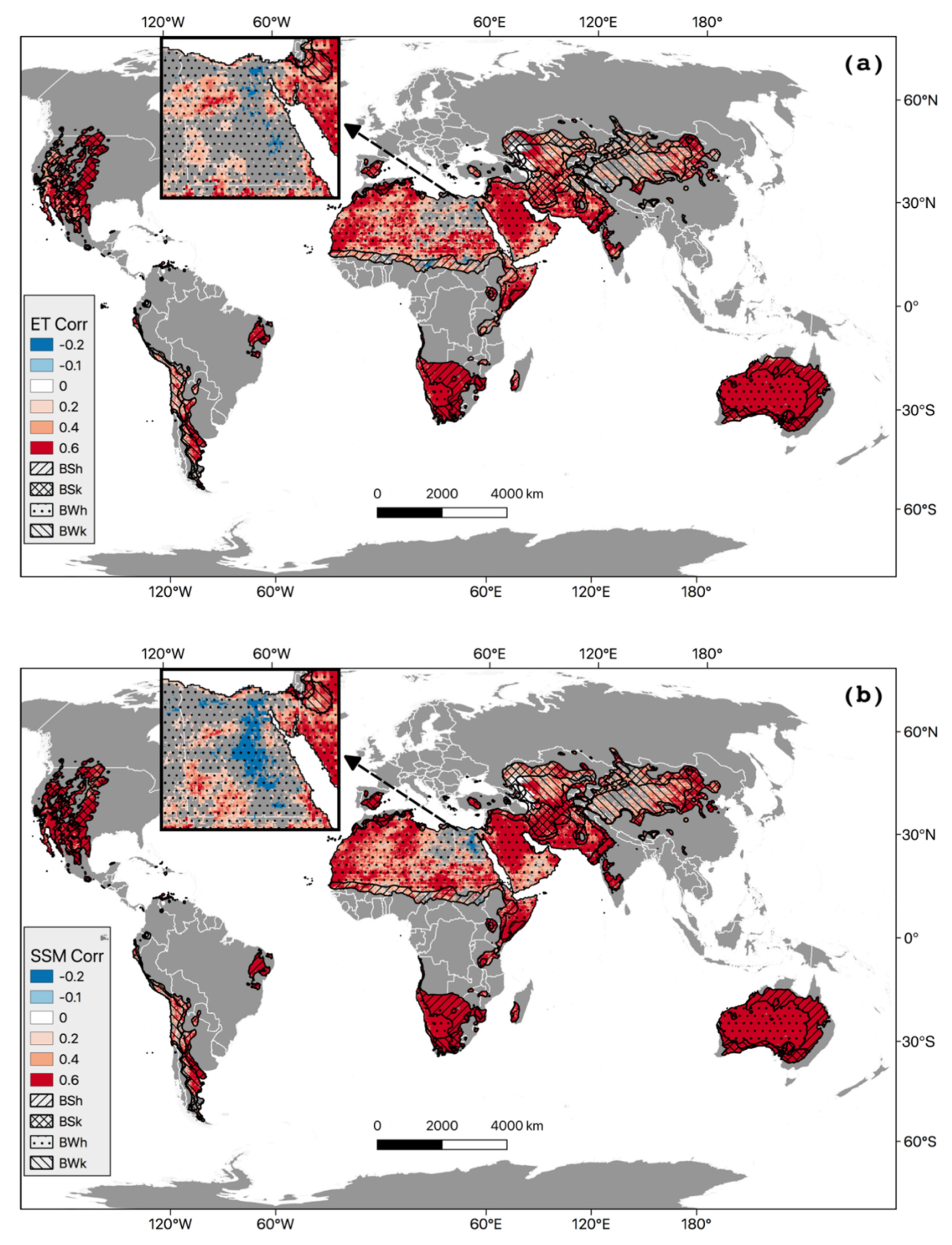
2.3.2. Correlational Analysis

For the purpose of finding the correlational relationship between the multiple variables, correlation maps were developed to show the standard correlation using the Pearson correlation coefficient ( r ) in the range from −1 (anti-correlation) to +1 (perfect correlation), between these two monthly time series x and y, with N elements as Equation (2):
r = i = 1 N ( x i x ¯ ) ( y i y ¯ ) i = 1 N ( x i x ¯ ) 2 i = 1 N ( y i y ¯ ) 2 = Cov ( x , y ) σ x σ y
with Cov being the covariance function, x ¯ and y ¯ the average and σ x and σ y the standard deviations for x and y, respectively.
In this study, the association between the GLDAS and FLDAS products in both SSM and ET variables over global arid and semi-arid regions was studied by the Pearson correlation analysis using their anomalies value X a calculated as Equation (3):
X a = X   X ¯
with X as the monthly value and X ¯ as the monthly mean value. The anomalies value X a can better demonstrate the effect of the change in a variable on the corresponding variable in the correlational analysis, especially when both variables have same pattern of seasonal variations. For instance, the correlation maps between the monthly anomalies values of Chlorophyll-a concentrations and environmental variables provided a better representation of their connections than simply using monthly mean values in [63,64].

2.3.3. Data-Driven Modelling of Selected Variables

In this study, the monthly data from dryland area in Egypt (mainly the Nile Delta region) during the years 2010 to 2019 were sampled and selected for the SSM and ET model development and evaluation. This region has 50 randomly selected sampling locations with a 10 km scale. A total of 29 parameters, including MODIS SSM and ET (modeling objective), as well as GLDAS and FLDAS outputs (e.g., Heat flux, specific humidity, total precipitation rate, soil temperature, wind speed, etc.) were used in the modelling (see comprehensive list in Table S1). The modelling dataset (~3000 records) was randomly split into a training set and testing set, with a ratio of 8:2, respectively.
Traditionally, intensive manual experiments are needed for model selection and parameterization, because it is difficult to know which model is most suitable for the problem before researchers try all the models. Therefore, the automatic optimization methods were proposed to overcome this issue, which try to train and evaluate model groups by parameters sequentially, and then include new parameter groups according to the updated results. In this study, automated model selection and tuning techniques were performed using Bayesian parameter optimization on the OptiML platform (https://bigml.com/api/optimls), which tried different supervised models (101 in total) for the regression tasks, including one linear regression, 89 tree models, 9 ensembles (up to 256 trees), and two deep neural networks. During the process, the platform used the Monte Carlo cross-validation [65], which iteratively generated new original data sets of training and test segmentation for the upper half of the model, and discarded the remaining half of the model due to poor performance. Therefore, this approach has an advantage over k-fold cross validation for the training and validation subsets, in that it is independent of the number of iterations. For both SSM and ET, deep neural networks outperformed other candidate models with R2 values of 0.87 and 0.81 (see comprehensive metrics in Table S2), respectively, and thus applied for the simulation.

2.3.4. Model Accuracy Assessment

Following [66], accuracy assessments of the algorithms are presented through standard statistical errors (root mean square error (RMSE), bias ( ψ ), the mean absolute percentage difference (|ψ|)), and the linear regression (i.e., slope, intercept, and coefficient of determination (R2)). Mathematically, the value of ψ is derived from the following:
ψ = 1 N i = 1 N ψ i
where N is the number of data points and ψ i is derived from:
ψ i = ( X s i m u l a t i o n   ( i ) X o b s   ( i ) X o b s   ( i ) ) × 100
In addition, the value of | ψ | is calculated from the following:
| ψ | = 1 N i = 1 N | ψ i |
The quantity ψ determines the bias, while | ψ | illustrates the scattering of data points.

3. Results

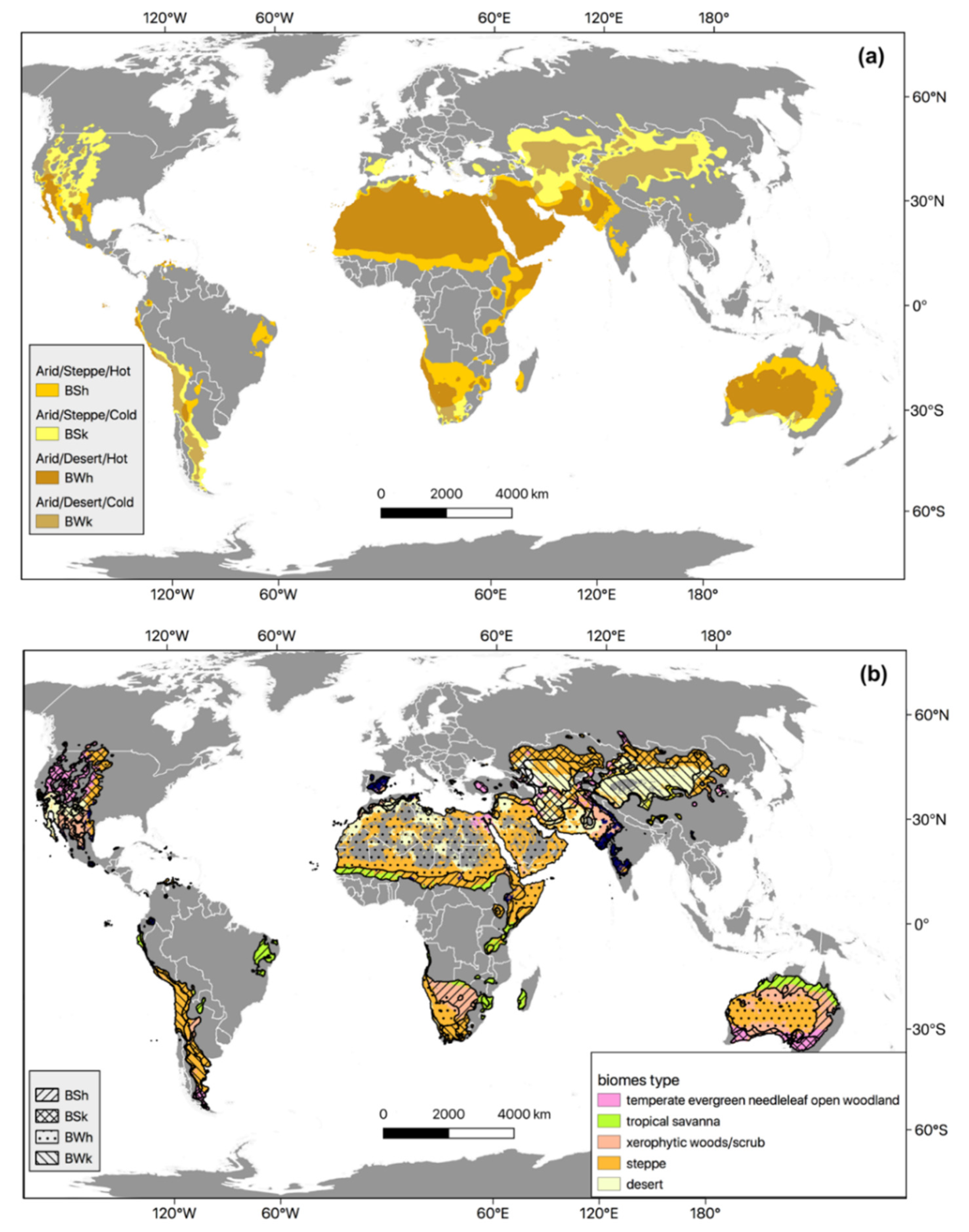
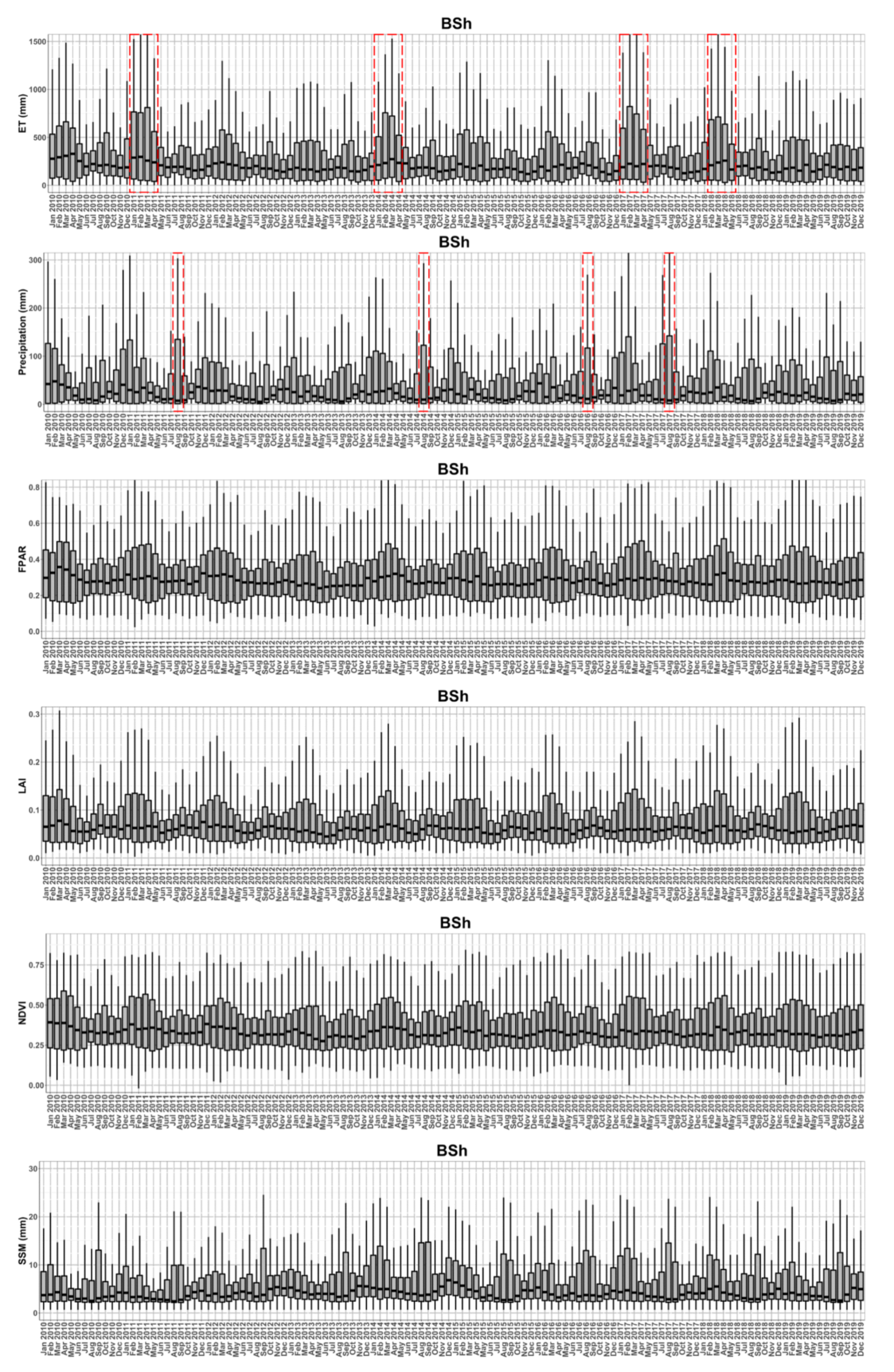
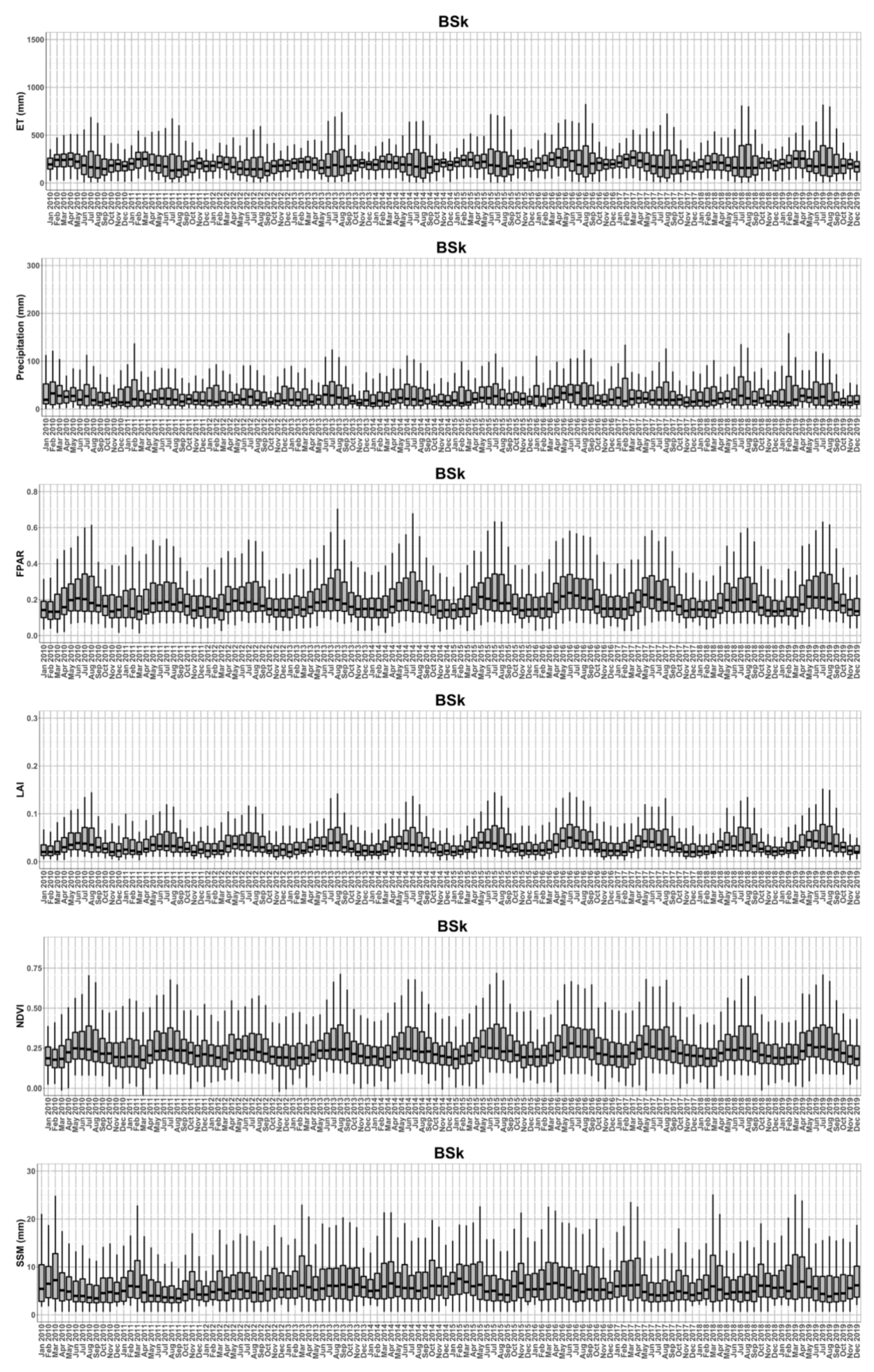
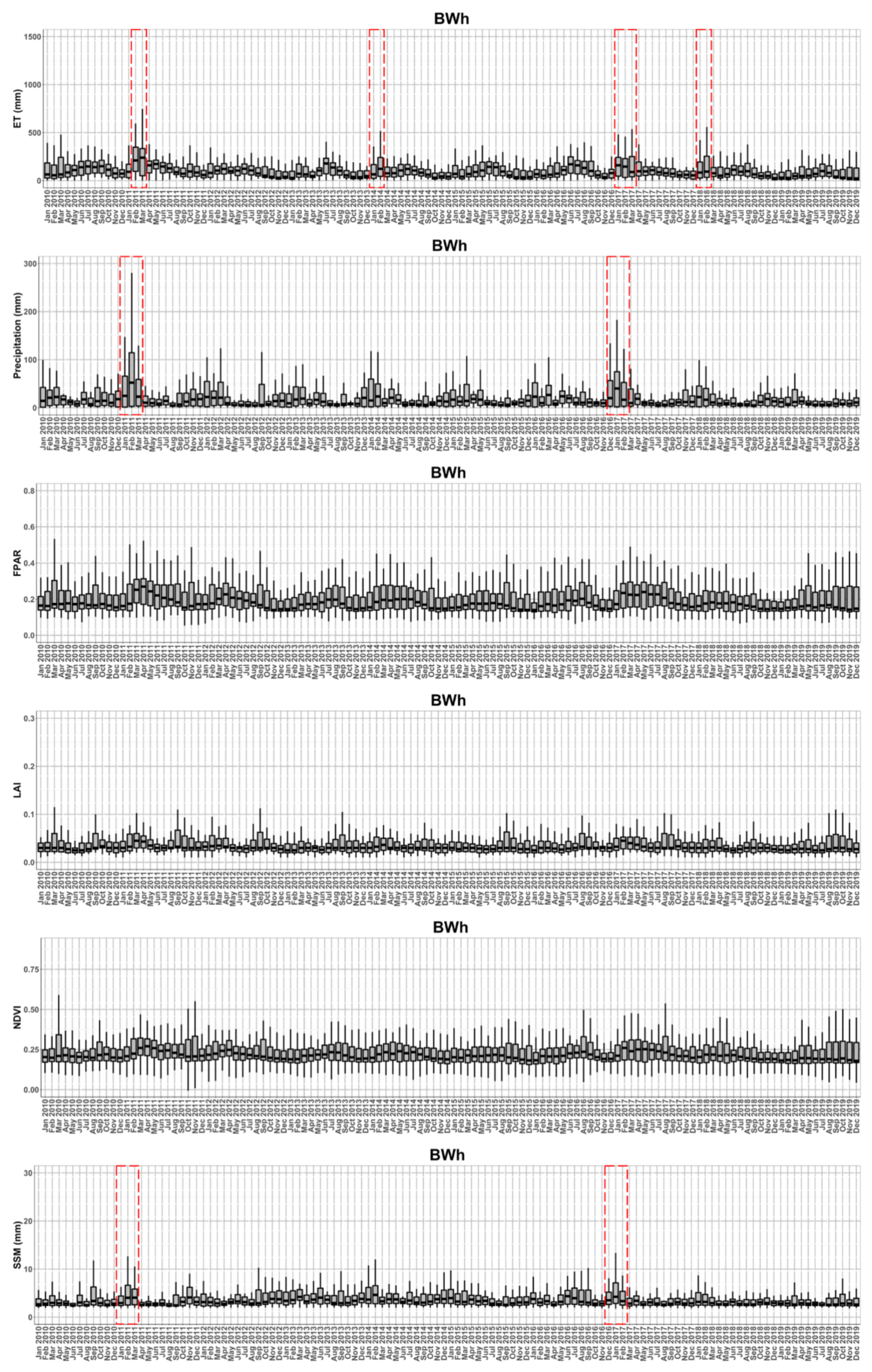
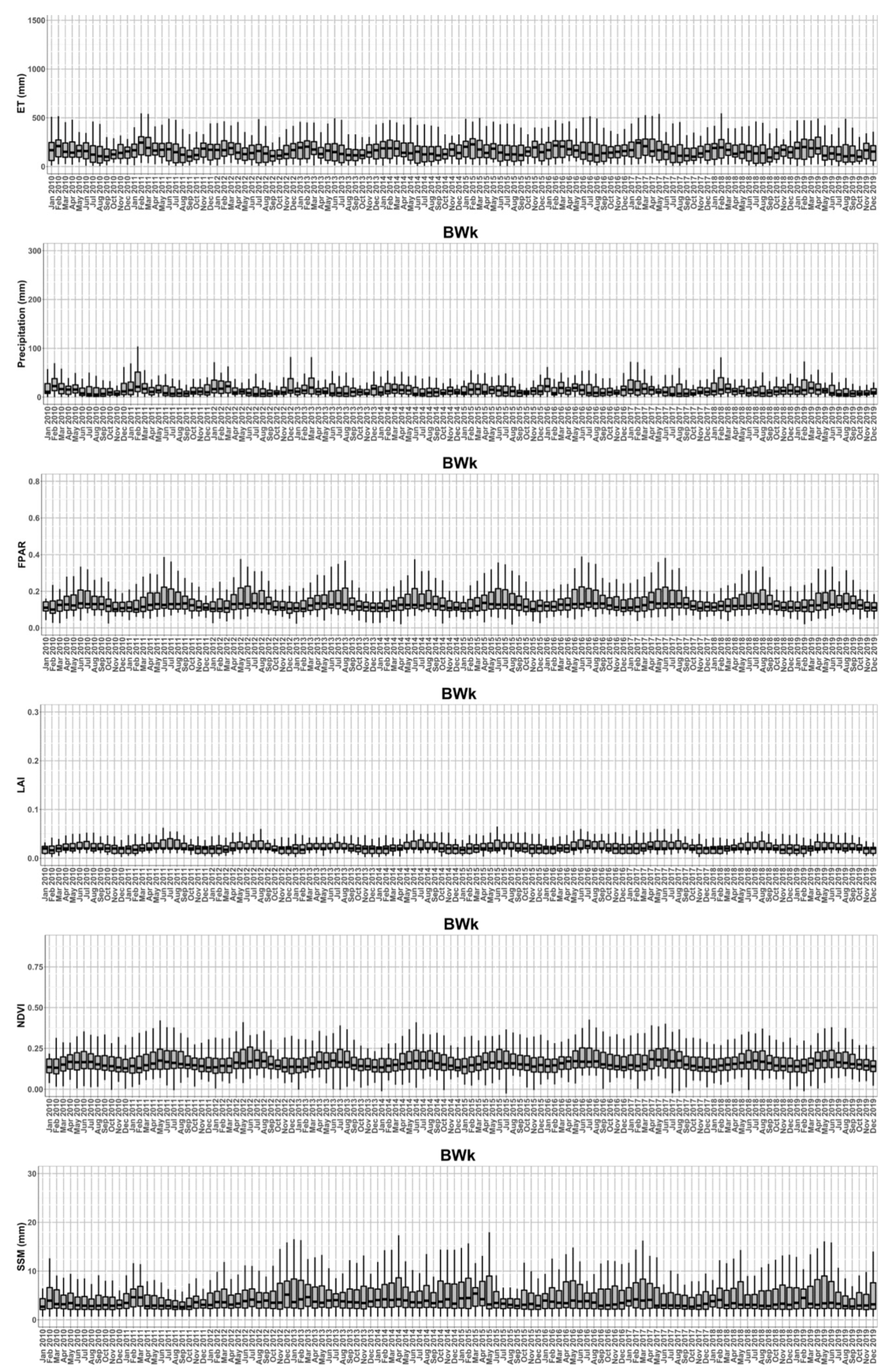
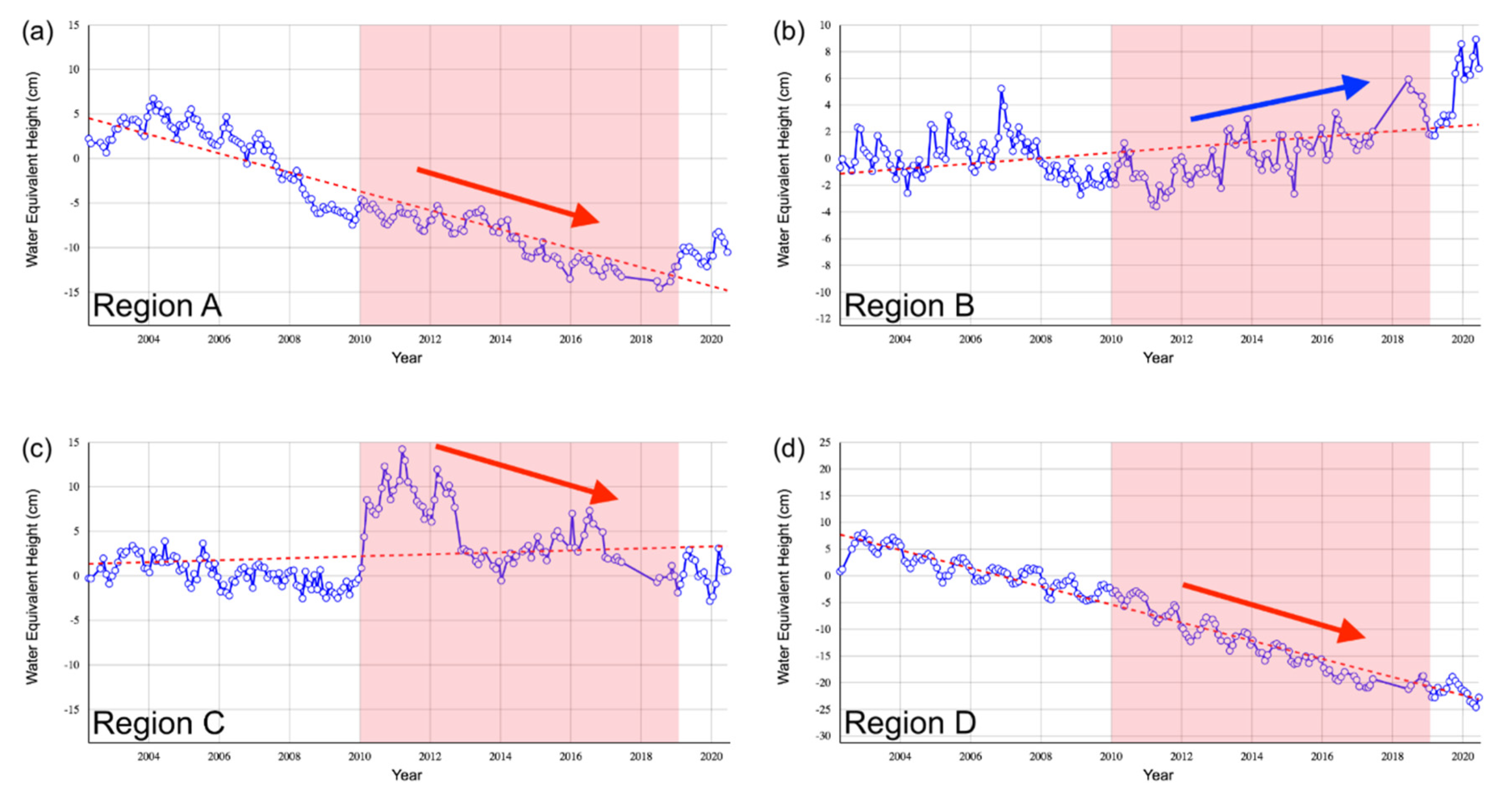
3.1. The Time Series of Multiple Hydrological Parameters

Time series boxplots of multiple variables, in the order of ET, precipitation, FPAR, LAI, NDVI and SSM (surface soil moisture), are presented in Figure 2, Figure 3, Figure 4 and Figure 5 for the BSh, BSk, BWh and BWk regions, respectively. Generally, the BSh region exhibits the highest values for all variables. On the other hand, the BWh region has the lowest ET and SSM, whereas the BWk region has the lowest FPAR, LAI, NDVI and precipitation. For BSh (Figure 2), strong seasonal patterns of ET are represented by maximum and upper quartile values: (1) highest in spring (February and March); (2) second highest in early fall (August and September); (3) lowest in June, July, October and November. Such patterns can also be found by median values, yet without peaks in early fall. The years of 2011, 2014, 2017 and 2018 (highlighted in Figure 2) show higher ET compared with other years. The seasonal variation is also shown in precipitation records, while the double peaks of maximum/upper quartile values are slightly changed, occurring often in winter (December to March) and later summer. The summer precipitation peaks sometimes surpassed the spring peaks (e.g., August in 2011, 2014, 2016 and 2017) (highlighted in Figure 2). For BSk (Figure 3), ET maximum/upper quartile values show a different seasonal pattern: (1) highest in summer (June, July and August); and (2) lowest in winter (December and January), indicating temperature as the controlling factor for ET. For both BSh and BSk, the FPAR, LAI and NDVI likely have the same patterns of seasonality as shown in ET and precipitation, while their SSM has comparably irregular seasonality patterns.
For BWh (Figure 4), due to lower overall ET, the seasonal pattern of median value is less noted, showing highest ET in summer (June and July), with occasional pulses in later winter and early spring (e.g., 2011, 2014, 2017 and 2018) (highlighted in Figure 4). The precipitation maximum and upper quartile values of BWh are highest in later winter and early spring. The strong precipitation pulses in 2011 and 2017 explain the ET surges at the same time. In contrast, BWk (Figure 5) has the highest ET in spring (February and March). In addition, the SSM of BWk indicates a dry period of 3 years from 2010 to 2012. For both BWh and BWk, their FPAR, LAI and NDVI do not show such seasonality pattern as shown by ET. However, the precipitation pulses in 2011 and 2017 are not reflected in these variables.

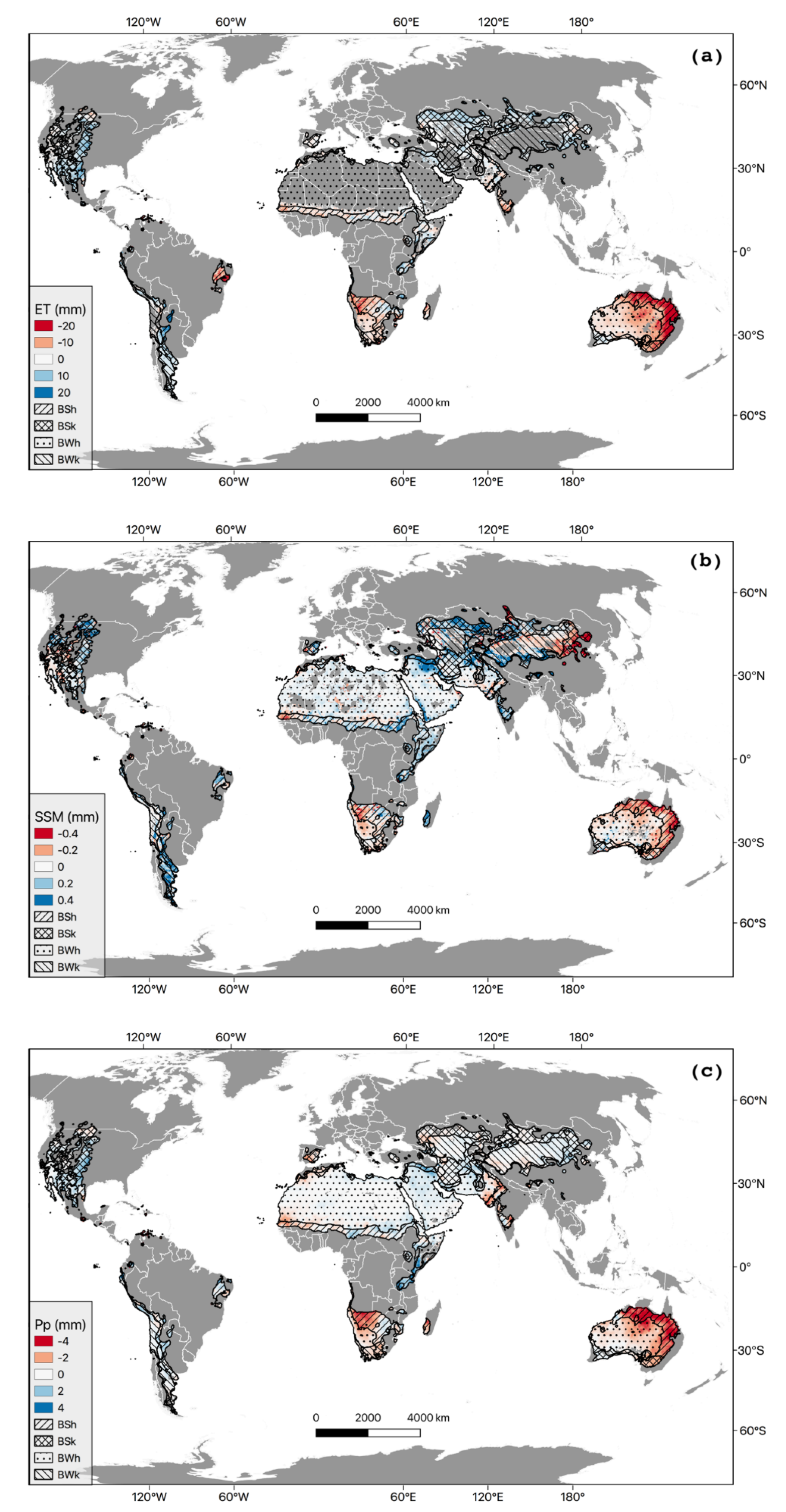
3.2. Trends of Multiple Hydrological Parameters

Figure 6 illustrates the trends followed by multiple variables, including ET (Figure 6a), SSM (Figure 6b) and precipitation (Pp) (Figure 6c) over BSh, BSk, BWh and BWk regions calculated based on harmonic analysis during the period between 2010 and 2019, only showing regions where the linear trend was statistically significant at the 95% confidence level. Comparing these data with Figure 1b, typical vegetation types of tropical savanna and scrub (BSh regions in the south of Africa and east of Australia) faced a rapid decreasing trend for all variables, indicating serious drought conditions. SSM also dropped in the north of China. Meanwhile, some regions experienced an increase in: (1) ET in the south of Argentina and Paraguay; (2) SSM in Eastern Europe and North America; (3) precipitation in North America (middle of the United States) and Eastern Africa (Tanzania). Colossal regions of the Middle East and North Africa (MENA), as well as the western desert of China, are absent in ET maps, due to the calculated trend not reaching the statistical significance level.

3.3. The Landcover and Water Storage Changes

Figure 7 shows the land cover changes between 2010 and 2019 over BSh, BSk, BWh and BWk regions. Table 1 shows the pixel count of the areas that changed and the percentages for each type: BSh has the highest change of 10.57%, while BWh has the lowest change of 3.92%. It is noted that such changes are most plausible in four regions: (1) Region A: north of Syria and Iraq in the Mesopotamia area; (2) Region B: east of Ethiopia and Somalia in Eastern Africa; (3) middle and east of Australia; and (4) Region D: south of Argentina. The time series plots in Figure 8 illustrate the GRACE Water Equivalent Height values in each region with the pink areas covering the periods from 2010 to 2019, which indicate different types of water storage changes: (1) Region A had a steady decrease from 2010 to 2019 until recent recovery in 2020; (2) Region B has been increasing since 2010; (3) Region C decreased from the historical peak in 2011 and returned to the average level; (4) Region D has experienced a continuous decrease since 2002.

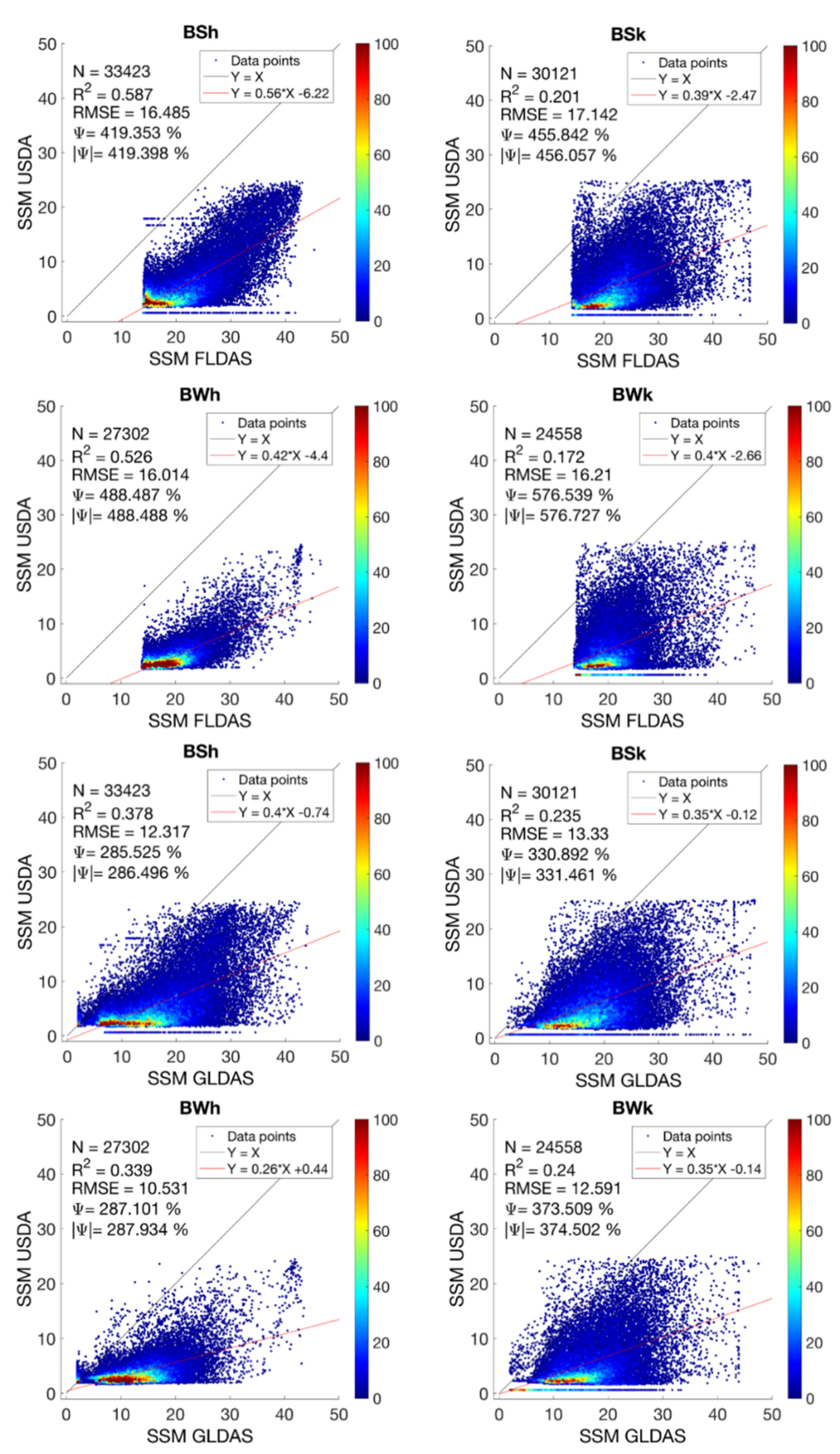
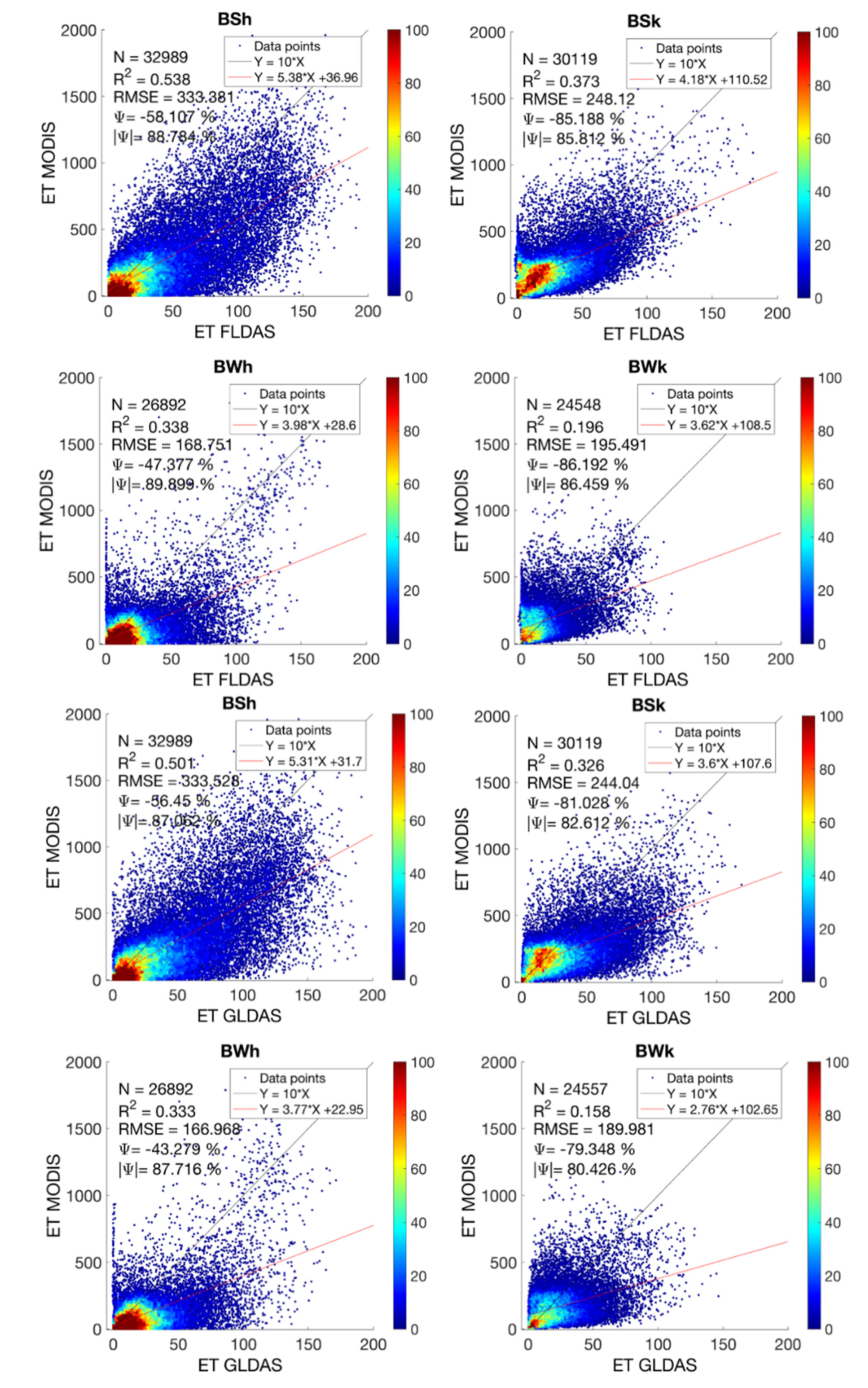
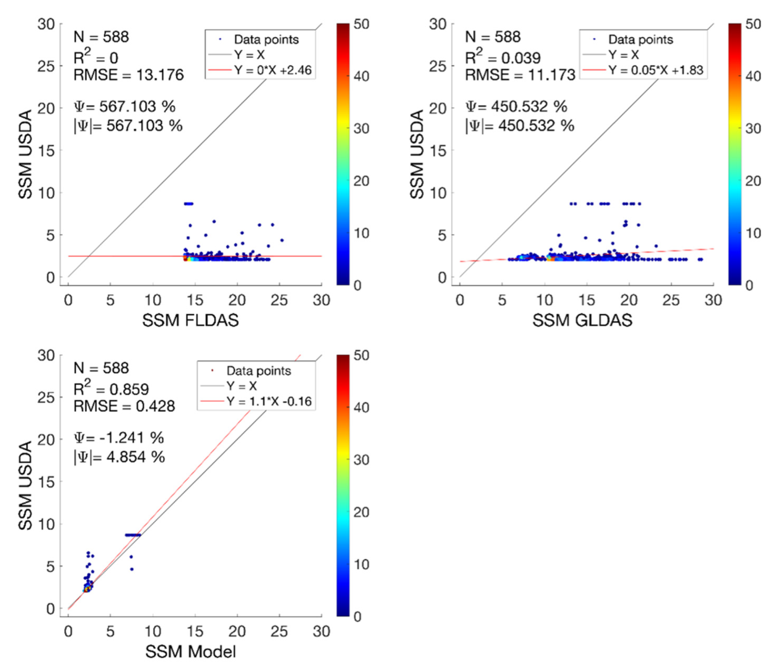
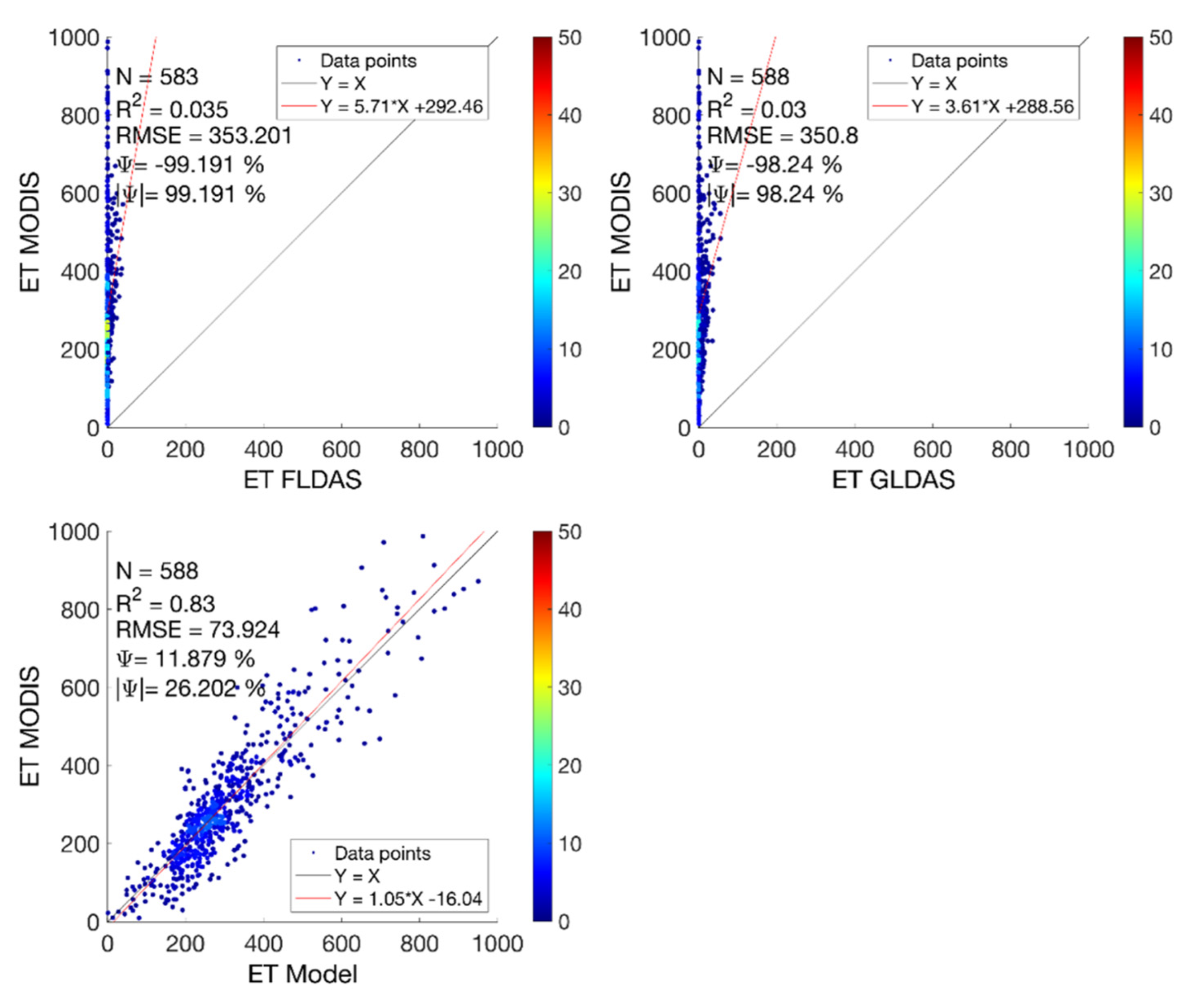
3.4. The Comparison and Modeling of FLDAS and GLDAS ET and SSM Products

Figure 9 shows correlation maps between FLDAS and GLDAS ET (Figure 9a) and SSM (Figure 9b) products. It is noted that some regions (areas in China, Egypt, Saudi Arabia) are not shown due to a lower confidence value (<95%) in the statistical significance test. In general, FLDAS ET/SSM products have strong consistency with those of GLDAS. However, some BWh and BWk regions (North Africa, south of the Arabian Peninsula, west of China, west coast of South America) demonstrate less correlation, while some areas in Egypt even showing a negative correlation (small map in Figure 9b). Compared with Figure 1b, these regions are mostly covered by desert or have no biome data recorded.
Moreover, the comparisons between satellite-based products (NASA-USDA SSM and MODIS ET) and model products obtained from FLDAS and GLDAS over arid regions (BSh, BSk, BWh and BWk) are presented in Figure 10 (SSM) and Figure 11 (ET), respectively. It is noted that both models tend to overestimate SSM (linear regression coefficient <1) but underestimate ET (linear regression coefficient >1), which is indicated by the positive (SSM) and negative (ET) biases ( ψ ). The values of | ψ | and ψ are nearly identical for all plots in Figure 10. The absolute values of ψ and | ψ | are also almost identical in the cold areas (BSK and BWk), while different in the hot areas (BSh and BWh). This means model outputs of ET sometimes are estimated as being higher than ET observed from MODIS satellites in the hot areas but not in the cold areas. For SSM products (Figure 10), satellite SSM values fall into the range of around [0, 25], while ranges of [12, 48] and [0, 45] are set for FLDAS and GLDAS, respectively. For both FLDAS and GLDAS, the hot areas (BSh and BWh) have better consistency with NASA-USDA products than the cold areas (BSK and BWk). Compared with GLDAS, FLDAS achieves better consistency in the hot areas with higher R2, yet is slightly worse in the cold areas. For ET products (Figure 11), the highest consistency is found in BSh, yet the lowest consistency in BWk. FLDAS has slightly better coherency with MODIS ET data than GLDAS in all regions.
As shown in Figure 9, strong disagreement between FLDAS and GLDAS products mainly exists in the Egypt territory. It is not decided which product has better performance due to a lack of ground observations. Therefore, the satellite-based dataset becomes a relatively reliable source of monitoring SSM and ET in this region. However, the satellite-based dataset is occasionally inaccessible due to atmospheric conditions (e.g., clouds) and sensor operating issues. Therefore, additional investigations are conducted in this region to compare FLDAS and GLDAS’s coherency with satellite products to improve their performance through machine learning modeling. Scatterplots are applied to compare the satellite products with FLDAS, GLDAS and the proposed model. The results are presented in Figure 12 and Figure 13 for SSM and ET, respectively. It is noted that both FLDAS and GLDAS have undesired results with near-zero R2 and high RMSE, | ψ | and ψ . The proposed models in this study remarkably improve the results with a very good correlation coefficient R2 (>0.8) and lower RMSE and bias.

4. Discussions

At local and regional scales, previous studies have been conducted on the connections between hydrological and environmental/climatic variations in arid and semi-arid regions. A study at China’s Yarlung Zangbo River (YLZR) basin showed the negatively correlated relationship between the climatic indices, including Pacific decadal oscillation (PDO) and the multivariate El Niño-Southern Oscillation (ENSO) index (MEI)) and precipitation, annual average temperature, and the streamflow of selected hydrological stations [67]. Similarly, this negative relationship between precipitation and ENSO indices was also found for Jana and Karan Islands in the nearshore Saudi Arabia area [36]. The monthly precipitation datasets (the time period 1961–2007) were compared over the arid Balochistan province of Pakistan, showing an increase in drought with global warming, indicated by the time series analysis of gauge-based records and climate models [68]. The study in the Upper Omo-Ghibe river basin of Ethiopia showed the trends in precipitation, temperature, and streamflow in the period from 1981 to 2008. A detailed review of the studies in global-scale monthly hydroclimatic time series was reported [69]. Therefore, our satellite-based approach on the analysis of monthly hydroclimatic time series during the last decade (2010–2019) is an updated continuing study of the dryland hydrology at a global scale. However, one of the fundamental challenges of dryland remote sensing is the decoupling of the ecosystem function (e.g., vegetation photosynthetic ability and stomatal conductance) from optical reflectance [70]. During the drought periods of extreme moisture shortage, some vegetation types, especially drought-tolerant evergreen shrubs, can keep constant greenness even if their vegetation and soil function decrease. This situation can be found in the boxplots in Figure 2, Figure 3, Figure 4 and Figure 5, where it is noted that the indices (FPAR, LAI and NDVI) do not have strong responses for ET as compared to the precipitation pulses. Additionally, high aerosol concentrations, leaves covered by dust, marked adjacency effect, as well as surface anisotropy in sparse and heterogeneous canopies, make high-quality surface reflectance retrievals over drylands still a challenging process [71,72,73]. In arid and semi-arid ecosystems, the presence of soil background, standing litter and senesced vegetation, can have a significant impact on the reflectance and vegetation indices (e.g., NDVI), also adding considerable noise to LAI and the retrieval of FPAR [74,75,76,77]. The spurious changes induced by variable soil background reflectance also make it difficult to validate the actual vegetation change [76,78,79]. Therefore, the Soil-Adjusted Vegetation Index (SAVI) was introduced with a soil adjustment factor (L), typically set as L = 0.5 [75], to account for differences from the soil background in red and near-infrared reflectance. However, SAVI is limited to differentiate vegetation from soil under sparse vegetation cover conditions [79]. Prior knowledge is also required to select the optimal L value [75]. In addition, one of the major assumptions of global MODIS LAI and FPAR products is that each pixel contains only one biome type with constant within-biome soil and vegetation properties [80]. However, this simplified assumption is unlikely to hold in arid and semi-arid areas due to their heterogeneous characteristics.
Sustainable water resources management requires knowledge regarding the effects of land use and land cover change (LULCC) on groundwater recharge and surface runoff [81]. The tropical and sub-tropical semi-arid regions use groundwater to meet improving urban, industrial and agricultural water requirements [82]. Hence, a thorough understanding of these effects and the subsequent changes is required to maintain a sustainable water supply in the arid and semi-arid regions. In response to the growing food demand of an increasing human population, semi-arid regions are experiencing a major conversion of natural vegetation to agricultural land, leading to land exploitation due to agricultural practices [83]. Figure 7 shows the situation of land cover changes over drylands, where some hotspot regions were also experiencing LULCC along with groundwater variations. Some regions in Iraq depend on groundwater for sprinkler irrigation to overcome the issue of less water due to a shortage of rainfall. Before this, groundwater was one of the main sources of freshwater and for domestic uses. Because of this change, many government and private wells have been drilled to use for irrigation [84]. In Syria, during the conflict with ISIS, the dependence on groundwater for agriculture grew at an alarming rate, as ISIS controlled the Euphrates river dam [85]. In many parts of Ethiopia, such as the Shinile catchment found in the Somali regional state, the pastoral and semi pastoral communities travel a long distance in search of water and grazing land. It is largely an arid and semi-arid watershed with a large potential for groundwater which the communities are unaware of [86]. New South Wales in Australia has undergone transitions between pasture/scrubland, vineyard and built-up land [87]. These transitions due to tourism and economic development would affect the groundwater recharge in the region. In Argentina, there is evidence of an increase in groundwater recharge in areas where croplands replaced forests [88]. Some studies also show that land cover changes influence ecosystem water fluxes as well as salinity patterns [89,90]. It is noted that land cover and groundwater change during the later 2010s is possibly connected with global warming conditions between 2014 and 2019, which are among the warmest years on record, and the year 2020 is likely to become the second warmest year on record (https://www.ncdc.noaa.gov/cag/global/haywood/globe/land_ocean).
Both GLDAS and FLDAS do provide a suite of outputs over a global domain in order to provide physically consistent and spatially and temporally continuous products that are critical for global dryland studies. In particular, FLDAS has been recommended in hydroclimate studies and early warning applications over areas of Eastern, Southern, and Western Africa [57]. However, in Figure 9, the strong discrepancy between GLDAS and FLDAS for certain areas excludes North Africa from the recommendatory list. The analysis in Figure 10 and Figure 11 shows the modeling biases in cold and dry areas from both FLDAS and GLDAS SSM/ET products, showing that they systematically overestimate the SSM and underestimate the ET, respectively. However, the higher SSM values from models may be due to their soil layer depth being configured as 0–10 cm, while the satellite generally detects the soil moisture at depths of 0-5cm. A study on the central Tibetan Plateau [91] suggested that the modeling biases were contributed by soil texture and soil organic carbon (SOC) content that alters soil thermal/hydraulic properties, which causes the significant underestimation of the surface soil moisture. The present study also suggested that products retrieved from the Advanced Microwave Scanning Radiometer-Earth Observing System (AMSR-E) evidently overestimated soil moisture, indicating that the satellite-based retrieval algorithms must be improved for the cold semi-arid regions. In arid and semi-arid ecosystems, it is still a theoretical and technical challenge to partition ecosystem scale ET fluxes between plant transpiration and soil/canopy evaporation [92]. Both numerical models and satellite products require ground-based data for calibration and validation. However, the observational data (chiefly from flux towers) are very limited, which results in inaccurate, poorly constrained estimates of energy, water, and carbon fluxes in the dryland to study its ecosystem’s structural and functional dynamics.
In Figure 12 and Figure 13, the proposed SSM/ET products by using machine-learning models demonstrate an appreciable improvement over the LDAS model. The previous studies applying similar automatic methodologies have been discussed [35,40,93], highlighting the importance of balancing the performance and explainability of the machine learning models for scientific studies. The machine learning models, along with numerical models based on physical processes (e.g., FLDAS), are the most important sources for hydrological studies in the dryland countries due to their limited scientific data and technological ability. For example, countries in the Nile River Basin (shared by Egypt, Sudan, Tanzania, Ethiopia, etc.) are undergoing accelerated population growth and urbanization [39]. The ongoing construction and filling of Ethiopia’s Grand Ethiopian Renaissance Dam have brought up intensifying tensions between Ethiopia and downstream dryland countries including Egypt and Sudan. However, scientific studies are restricted to support the decision making and collaborations due to limited on-site observations, while the number of functional hydrometeorological gauging stations declined by 88% between the early 1960s and 2014 [94]. It is noted that our approach to the correction of the process-based hydrological models is also known as a process of hydrological post-processing to obtain “point” predictions. By contrast, new data-driven practices [95,96] of delivering “probabilistic” hydrological predictions (e.g., quantile regression [97]) were introduced recently with their potential in expressing complex hydrological processes considering predictive uncertainties [98].
Fortunately, new and emerging advances leverage significant opportunities for overcoming previous challenges in dryland remote sensing and thus revolutionize our ability to contextualize arid and semi-arid regions within the broader Earth system. Accordingly, the following strategies are recommended [99]: (1) exploring novel fusions of sensors and techniques across different spatiotemporal scales (e.g., solar-induced fluorescence, thermal, microwave, hyperspectral, and LiDAR) to understand dryland structural and functional dynamics; (2) capturing instant responses of dryland ecosystems to diurnal variation in water stress by utilizing near-continuous observations from geostationary satellites; (3) building up new ground observational networks for validation and calibration to better represent the heterogeneity of dryland system; (4) developing algorithms specifically for dryland ecosystems; (5) coupling physical process-based models with remote sensing observations using data assimilation to improve ecological forecasts and long-term projections.

5. Conclusions

In this paper, we investigated the hydrological conditions over global arid and semi-arid regions, including areas of BSh (Hot semi-arid climate), BSk (Cold semi-arid climate), BWh (Hot desert climate) and BWk (Cold desert climate), through synergistic approaches of remote sensing and modelling. The time series analysis during the last decade (2010–2019) of multiple hydrological variables (ET, SSM and precipitation) and vegetation indices (FPAR, LAI and NDVI) highlighted precipitation pulses that showed less impact on the vegetation indices compared to ET and SSM in some arid regions. Moreover, the trends of ET, SSM and precipitation, as well as land cover changes, that were demonstrated over the same period, emphasized drier trends in the south of Africa and the east of Australia and wetter trends in Mesopotamia and North America. Finally, the comparison of widely-used FLDAS and GLDAS models showed a general consistency, while a strong discrepancy was observed in the downstream Nile Basin, also demonstrating the fact that both LDAS models overestimate SSM and underestimate ET while model outputs of hot areas have better consistency with satellite products than cold areas.
This work further confirmed the scientific fact of decoupling between ecosystem function and observed optical characteristics (e.g., greenness indicated by vegetation indices), which calls for novel techniques and applications of remote sensing in the arid and semi-arid regions. Some areas (e.g., Mesopotamia, Eastern Africa, Australia and Argentina) experienced intense land cover changes along with noted water storage variations, indicating complex hydrological processes which need further investigations. Our data-driven modelling as a post-processing approach effectively improved the process-based models’ performance and recommended that both process-based and satellite-based hydrological products have a higher potential to be improved for the arid and semi-arid regions. However, considering complex hydrological processes and predictions uncertainties, new practices of delivering data-driven probabilistic modelling are suggested for future studies. In addition, the study was fully deployed on the open-source cloud computing and analytical platforms (Google Earth Engine and BigML), which posed their great potential in other global-scale environmental studies.

Supplementary Materials

The following are available online at https://www.mdpi.com/2072-4292/12/23/3973/s1, Table S1: Selected Variables for the Data-driven Machine Learning Modelling, Table S2: The metrics of selected models for SSM and ET.

Author Contributions

Conceptualization, H.E.-A. and W.L.; data analysis, W.L. and R.T.; funding acquisition, H.E.-A.; methodology, H.E.-A., W.L. and R.T.; validation, W.L. and R.T.; writing—original draft, H.E.-A., W.L.; writing—review and editing, H.E.-A., W.L., R.T., T.P., S.P.T., K.P.M. and D.S. All authors have read and agreed to the published version of the manuscript.

Funding

Rejoice Thomas would like to acknowledge the support from the Earth Systems Science and Data Solutions (EssDs) Lab and the Computational and Data Sciences Graduate Program, Schmid College of Science and Technology, Chapman University.

Acknowledgments

The first author acknowledge the support from the Earth Systems Science and Data Solutions (EssDs) Lab and Schmid College of Science and Technology, Chapman University.

Conflicts of Interest

The authors declare no conflict of interest.

References

  1. Assessment, M.E. Dryland Systems, Ecosystems and Human Well-Being: Current State and Trends; Island Press: Washington, DC, USA, 2005. [Google Scholar]
  2. Ahlstrom, A.; Raupach, M.R.; Schurgers, G.; Smith, B.; Arneth, A.; Jung, M.; Reichstein, M.; Canadell, J.G.; Friedlingstein, P.; Jain, A.K.; et al. The dominant role of semi-arid ecosystems in the trend and variability of the land CO2 sink. Science 2015, 348, 895–899. [Google Scholar] [CrossRef] [Green Version]
  3. Biederman, J.A.; Scott, R.L.; Bell, T.W.; Bowling, D.R.; Dore, S.; Garatuza-Payan, J.; Kolb, T.E.; Krishnan, P.; Krofcheck, D.J.; Litvak, M.E.; et al. CO2 exchange and evapotranspiration across dryland ecosystems of southwestern North America. Glob. Chang. Biol. 2017, 23, 4204–4221. [Google Scholar] [CrossRef]
  4. Humphrey, V.; Zscheischler, J.; Ciais, P.; Gudmundsson, L.; Sitch, S.; Seneviratne, S.I. Sensitivity of atmospheric CO2 growth rate to observed changes in terrestrial water storage. Nature 2018, 560, 628–631. [Google Scholar] [CrossRef]
  5. Poulter, B.; Frank, D.; Ciais, P.; Myneni, R.B.; Andela, N.; Bi, J.; Broquet, G.; Canadell, J.G.; Chevallier, F.; Liu, Y.Y.; et al. Contribution of semi-arid ecosystems to interannual variability of the global carbon cycle. Nature 2014, 509, 600–603. [Google Scholar] [CrossRef] [Green Version]
  6. Huang, J.; Guan, X.; Ji, F. Enhanced cold-season warming in semi-arid regions. Atmos. Chem. Phys. 2012, 12, 5391–5398. [Google Scholar] [CrossRef] [Green Version]
  7. Huang, J.; Yu, H.; Guan, X.; Wang, G.; Guo, R. Accelerated dryland expansion under climate change. Nat. Clim. Chang. 2016, 6, 166–171. [Google Scholar] [CrossRef]
  8. Cayan, D.R.; Das, T.; Pierce, D.W.; Barnett, T.P.; Tyree, M.; Gershunov, A. Future dryness in the southwest US and the hydrology of the early 21st century drought. Proc. Natl. Acad. Sci. USA 2010, 107, 21271–21276. [Google Scholar] [CrossRef] [PubMed] [Green Version]
  9. Cook, B.I.; Ault, T.R.; Smerdon, J.E. Unprecedented 21st century drought risk in the American Southwest and Central Plains. Sci. Adv. 2015, 1, e1400082. [Google Scholar] [CrossRef] [PubMed] [Green Version]
  10. Huang, J.; Yu, H.; Dai, A.; Wei, Y.; Kang, L. Drylands face potential threat under 2 °C global warming target. Nat. Clim. Chang. 2017, 7, 417–422. [Google Scholar] [CrossRef]
  11. D’Odorico, P.; Porporato, A. (Eds.) Dryland Ecohydrology; Kluwer Academic Publishers: Dordrecht, The Netherlands, 2006; ISBN 978-1-4020-4259-1. [Google Scholar]
  12. Scott, R.L.; Huxman, T.E.; Barron-Gafford, G.A.; Darrel Jenerette, G.; Young, J.M.; Hamerlynck, E.P. When vegetation change alters ecosystem water availability. Glob. Chang. Biol. 2014, 20, 2198–2210. [Google Scholar] [CrossRef] [PubMed]
  13. Noy-Meir, I. Desert Ecosystems: Environment and Producers. Annu. Rev. Ecol. Syst. 1973, 4, 25–51. [Google Scholar] [CrossRef]
  14. Reynolds, J.F.; Smith, D.M.S.; Lambin, E.F.; Turner, B.L.; Mortimore, M.; Batterbury, S.P.J.; Downing, T.E.; Dowlatabadi, H.; Fernandez, R.J.; Herrick, J.E.; et al. Global Desertification: Building a Science for Dryland Development. Science 2007, 316, 847–851. [Google Scholar] [CrossRef] [Green Version]
  15. Nagler, P.L.; Nguyen, U.; Bateman, H.L.; Jarchow, C.J.; Glenn, E.P.; Waugh, W.J.; van Riper, C. Northern tamarisk beetle (Diorhabda carinulata) and tamarisk (Tamarix spp.) interactions in the Colorado River basin: Northern tamarisk beetle and tamarisk interactions. Restor. Ecol. 2018, 26, 348–359. [Google Scholar] [CrossRef]
  16. Nagler, P.L.; Jarchow, C.J.; Glenn, E.P. Remote sensing vegetation index methods to evaluate changes in greenness and evapotranspiration in riparian vegetation in response to the Minute 319 environmental pulse flow to Mexico. Proc. IAHS 2018, 380, 45–54. [Google Scholar] [CrossRef]
  17. Fisher, J.B.; Melton, F.; Middleton, E.; Hain, C.; Anderson, M.; Allen, R.; McCabe, M.F.; Hook, S.; Baldocchi, D.; Townsend, P.A.; et al. The future of evapotranspiration: Global requirements for ecosystem functioning, carbon and climate feedbacks, agricultural management, and water resources: The Future of Evapotranspiration. Water Resour. Res. 2017, 53, 2618–2626. [Google Scholar] [CrossRef]
  18. Baldocchi, D.; Falge, E.; Gu, L.; Olson, R.; Hollinger, D.; Running, S.; Anthoni, P.; Bernhofer, C.; Davis, K.; Evans, R.; et al. FLUXNET: A new tool to study the temporal and spatial variability of ecosystem-scale carbon dioxide, water vapor, and energy flux densities. Bull. Am. Meteorol. Soc. 2001, 82, 2415–2434. [Google Scholar] [CrossRef]
  19. Novick, K.A.; Biederman, J.A.; Desai, A.R.; Litvak, M.E.; Moore, D.J.P.; Scott, R.L.; Torn, M.S. The AmeriFlux network: A coalition of the willing. Agric. For. Meteorol. 2018, 249, 444–456. [Google Scholar] [CrossRef] [Green Version]
  20. Mirtl, M.; Borer, E.T.; Djukic, I.; Forsius, M.; Haubold, H.; Hugo, W.; Jourdan, J.; Lindenmayer, D.; McDowell, W.H.; Muraoka, H.; et al. Genesis, goals and achievements of Long-Term Ecological Research at the global scale: A critical review of ILTER and future directions. Sci. Total Environ. 2018, 626, 1439–1462. [Google Scholar] [CrossRef]
  21. Schimel, D.; Hargrove, W.; Hoffman, F.; MacMahon, J. NEON: A hierarchically designed national ecological network. Front. Ecol. Environ. 2007, 5, 59. [Google Scholar] [CrossRef]
  22. Kowalik, W.S.; Marsh, S.E.; Lyon, R.J.P. A relation between landsat digital numbers, surface reflectance, and the cosine of the solar zenith angle. Remote Sens. Environ. 1982, 12, 39–55. [Google Scholar] [CrossRef]
  23. Marsh, S.E.; Lyon, R.J.P. Quantitative relationships of near-surface spectra to Landsat radiometric data. Remote Sens. Environ. 1980, 10, 241–261. [Google Scholar] [CrossRef]
  24. Rouse, J., Jr. Contractor Report (CR): Monitoring the Vernal Advancement and Retrogradation (Green Wave Effect) of Natural Vegetation; NTRS—NASA Technical Reports Server: Washington, DC, USA, 1974.
  25. Tucker, C.J. Red and photographic infrared linear combinations for monitoring vegetation. Remote Sens. Environ. 1979, 8, 127–150. [Google Scholar] [CrossRef] [Green Version]
  26. Anyamba, A.; Tucker, C.J. Analysis of Sahelian vegetation dynamics using NOAA-AVHRR NDVI data from 1981–2003. J. Arid Environ. 2005, 63, 596–614. [Google Scholar] [CrossRef]
  27. Donohue, R.J.; McVicar, T.R.; Roderick, M.L. Climate-related trends in Australian vegetation cover as inferred from satellite observations, 1981–2006. Glob. Chang. Biol. 2009, 15, 1025–1039. [Google Scholar] [CrossRef]
  28. Fensholt, R.; Rasmussen, K. Analysis of trends in the Sahelian ‘rain-use efficiency’ using GIMMS NDVI, RFE and GPCP rainfall data. Remote Sens. Environ. 2011, 115, 438–451. [Google Scholar] [CrossRef]
  29. Donohue, R.J.; Roderick, M.L.; McVicar, T.R.; Farquhar, G.D. Impact of CO2 fertilization on maximum foliage cover across the globe’s warm, arid environments: CO2 Fertilization and Foliage Cover. Geophys. Res. Lett. 2013, 40, 3031–3035. [Google Scholar] [CrossRef] [Green Version]
  30. Fensholt, R.; Langanke, T.; Rasmussen, K.; Reenberg, A.; Prince, S.D.; Tucker, C.; Scholes, R.J.; Le, Q.B.; Bondeau, A.; Eastman, R.; et al. Greenness in semi-arid areas across the globe 1981–2007—An Earth Observing Satellite based analysis of trends and drivers. Remote Sens. Environ. 2012, 121, 144–158. [Google Scholar] [CrossRef]
  31. Helldén, U.; Tottrup, C. Regional desertification: A global synthesis. Glob. Planet. Chang. 2008, 64, 169–176. [Google Scholar] [CrossRef]
  32. Kolby Smith, W.; Reed, S.C.; Cleveland, C.C.; Ballantyne, A.P.; Anderegg, W.R.L.; Wieder, W.R.; Liu, Y.Y.; Running, S.W. Large divergence of satellite and Earth system model estimates of global terrestrial CO2 fertilization. Nat. Clim. Chang. 2016, 6, 306–310. [Google Scholar] [CrossRef]
  33. Zhu, Z.; Piao, S.; Myneni, R.B.; Huang, M.; Zeng, Z.; Canadell, J.G.; Ciais, P.; Sitch, S.; Friedlingstein, P.; Arneth, A.; et al. Greening of the Earth and its drivers. Nat. Clim. Chang. 2016, 6, 791–795. [Google Scholar] [CrossRef]
  34. Gorelick, N.; Hancher, M.; Dixon, M.; Ilyushchenko, S.; Thau, D.; Moore, R. Google Earth Engine: Planetary-scale geospatial analysis for everyone. Remote Sens. Environ. 2017, 202, 18–27. [Google Scholar] [CrossRef]
  35. El-Nadry, M.; Li, W.; El-Askary, H.; Awad, M.A.; Mostafa, A.R. Urban Health Related Air Quality Indicators over the Middle East and North Africa Countries Using Multiple Satellites and AERONET Data. Remote Sens. 2019, 11, 2096. [Google Scholar] [CrossRef] [Green Version]
  36. Maneja, R.H.; Miller, J.D.; Li, W.; El-Askary, H.; Flandez, A.V.B.; Dagoy, J.J.; Alcaria, J.F.A.; Basali, A.U.; Al-Abdulkader, K.A.; Loughland, R.A.; et al. Long-term NDVI and recent vegetation cover profiles of major offshore island nesting sites of sea turtles in Saudi waters of the northern Arabian Gulf. Ecol. Indic. 2020, 117, 106612. [Google Scholar] [CrossRef]
  37. Li, W.; El-Askary, H.; Qurban, M.A.; Li, J.; ManiKandan, K.P.; Piechota, T. Using multi-indices approach to quantify mangrove changes over the Western Arabian Gulf along Saudi Arabia coast. Ecol. Indic. 2019, 102, 734–745. [Google Scholar] [CrossRef]
  38. Li, W.; El-Askary, H.M.; Qurban, M.; Allali, M.; Manikandan, K. On the drying trends over the MENA countries using harmonic analysis of the enhanced vegetation index. In Advances in Remote Sensing and Geo Informatics Applications; El-Askary, H.M., Lee, S., Heggy, E., Pradhan, B., Eds.; Springer: Cham, Switzerland, 2019; pp. 243–245. ISBN 978-3-030-01439-1. [Google Scholar]
  39. Li, W.; El-Askary, H.; Lakshmi, V.; Piechota, T.; Struppa, D. Earth Observation and Cloud Computing in Support of Two Sustainable Development Goals for the River Nile Watershed Countries. Remote Sens. 2020, 12, 1391. [Google Scholar] [CrossRef]
  40. Li, W.; Ali, E.; Abou El-Magd, I.; Mourad, M.M.; El-Askary, H. Studying the Impact on Urban Health over the Greater Delta Region in Egypt Due to Aerosol Variability Using Optical Characteristics from Satellite Observations and Ground-Based aeronet Measurements. Remote Sens. 2019, 11, 1998. [Google Scholar] [CrossRef] [Green Version]
  41. Bastin, J.-F.; Berrahmouni, N.; Grainger, A.; Maniatis, D.; Mollicone, D.; Moore, R.; Patriarca, C.; Picard, N.; Sparrow, B.; Abraham, E.M.; et al. The extent of forest in dryland biomes. Science 2017, 356, 635–638. [Google Scholar] [CrossRef] [Green Version]
  42. Beck, H.E.; Zimmermann, N.E.; McVicar, T.R.; Vergopolan, N.; Berg, A.; Wood, E.F. Present and future Köppen-Geiger climate classification maps at 1-km resolution. Sci. Data 2018, 5, 180214. [Google Scholar] [CrossRef] [Green Version]
  43. Hengl, T.; Walsh, M.G.; Sanderman, J.; Wheeler, I.; Harrison, S.P.; Prentice, I.C. Global mapping of potential natural vegetation: An assessment of Machine Learning algorithms for estimating land potential. PeerJ 2018, 6, e5457. [Google Scholar] [CrossRef] [Green Version]
  44. Funk, C.; Peterson, P.; Landsfeld, M.; Pedreros, D.; Verdin, J.; Shukla, S.; Husak, G.; Rowland, J.; Harrison, L.; Hoell, A.; et al. The climate hazards infrared precipitation with stations—A new environmental record for monitoring extremes. Sci. Data 2015, 2, 150066. [Google Scholar] [CrossRef] [Green Version]
  45. Bolten, J.D.; Crow, W.T.; Zhan, X.; Jackson, T.J.; Reynolds, C.A. Evaluating the Utility of Remotely Sensed Soil Moisture Retrievals for Operational Agricultural Drought Monitoring. IEEE J. Sel. Top. Appl. Earth Obs. Remote Sens. 2010, 3, 57–66. [Google Scholar] [CrossRef] [Green Version]
  46. Mladenova, I.E.; Bolten, J.D.; Crow, W.T.; Anderson, M.C.; Hain, C.R.; Johnson, D.M.; Mueller, R. Intercomparison of Soil Moisture, Evaporative Stress, and Vegetation Indices for Estimating Corn and Soybean Yields Over the U.S. IEEE J. Sel. Top. Appl. Earth Obs. Remote Sens. 2017, 10, 1328–1343. [Google Scholar] [CrossRef]
  47. Mohammed, I.; Bolten, J.; Srinivasan, R.; Lakshmi, V. Improved Hydrological Decision Support System for the Lower Mekong River Basin Using Satellite-Based Earth Observations. Remote Sens. 2018, 10, 885. [Google Scholar] [CrossRef] [PubMed] [Green Version]
  48. Kerr, Y.H.; Levine, D. Foreword to the Special Issue on the Soil Moisture and Ocean Salinity (SMOS) Mission. IEEE Trans. Geosci. Remote Sens. 2008, 46, 583–585. [Google Scholar] [CrossRef]
  49. Landerer, F.W.; Swenson, S.C. Accuracy of scaled GRACE terrestrial water storage estimates: Accuracy of GRACE-TWS. Water Resour. Res. 2012, 48. [Google Scholar] [CrossRef]
  50. Swenson, S.; Wahr, J. Post-processing removal of correlated errors in GRACE data. Geophys. Res. Lett. 2006, 33, L08402. [Google Scholar] [CrossRef]
  51. Swenson, S. GRACE Monthly Land Water Mass Grids Netcdf Release 5.0; PO.DAAC: Pasadena, CA, USA, 2012.
  52. Mu, Q.; Zhao, M.; Running, S.W. MODIS Global Terrestrial Evapotranspiration (ET) Product (NASA MOD16A2/A3) Collection 5. NASA Headquarters; Report; Numerical Terradynamic Simulation Group Publications: Missoula, MT, USA, 2013. [Google Scholar]
  53. Didan, K. MOD13A2 MODIS/Terra Vegetation Indices 16-Day L3 Global 1 km SIN Grid V006; NASA LP DAAC: Washington, DC, USA, 2015. [CrossRef]
  54. Myneni, R. MOD15A2H MODIS/Terra Leaf Area Index/FPAR 8-Day L4 Global 500 m SIN Grid V006; NASA LP DAAC: Washington, DC, USA, 2015. [CrossRef]
  55. Chen, J.M.; Black, T.A. Defining leaf area index for non-flat leaves. Plant Cell Environ. 1992, 15, 421–429. [Google Scholar] [CrossRef]
  56. Fensholt, R.; Sandholt, I.; Rasmussen, M.S. Evaluation of MODIS LAI, fAPAR and the relation between fAPAR and NDVI in a semi-arid environment using in situ measurements. Remote Sens. Environ. 2004, 91, 490–507. [Google Scholar] [CrossRef]
  57. McNally, A.; Arsenault, K.; Kumar, S.; Shukla, S.; Peterson, P.; Wang, S.; Funk, C.; Peters-Lidard, C.D.; Verdin, J.P. A land data assimilation system for sub-Saharan Africa food and water security applications. Sci. Data 2017, 4, 170012. [Google Scholar] [CrossRef] [Green Version]
  58. Derber, J.C.; Parrish, D.F.; Lord, S.J. The new global operational analysis system at the National Meteorological Center. Weather Forecast. 1991, 6, 538–547. [Google Scholar] [CrossRef] [Green Version]
  59. Adler, R.F.; Huffman, G.J.; Chang, A.; Ferraro, R.; Xie, P.-P.; Janowiak, J.; Rudolf, B.; Schneider, U.; Curtis, S.; Bolvin, D.; et al. The version-2 global precipitation climatology project (GPCP) monthly precipitation analysis (1979–present). J. Hydrometeorol. 2003, 4, 1147–1167. [Google Scholar] [CrossRef]
  60. NASA GSFC Hydrological Sciences Laboratory (HSL). FLDAS Noah Land Surface Model L4 Global Monthly 0.1 × 0.1 Degree (MERRA-2 and CHIRPS) V001; Amy McNally NASA/GSFC/HSL: Greenbelt, MD, USA, 2018.
  61. Xie, P.; Arkin, P.A. Global precipitation: A 17-year monthly analysis based on gauge observations, satellite estimates, and numerical model outputs. Bull. Am. Meteorol. Soc. 1997, 78, 2539–2558. [Google Scholar] [CrossRef]
  62. Sheffield, J.; Goteti, G.; Wood, E.F. Development of a 50-Year High-Resolution Global Dataset of Meteorological Forcings for Land Surface Modeling. J. Clim. 2006, 19, 3088–3111. [Google Scholar] [CrossRef] [Green Version]
  63. Li, W.; El-Askary, H.; Qurban, M.; Proestakis, E.; Garay, M.; Kalashnikova, O.; Amiridis, V.; Gkikas, A.; Marinou, E.; Piechota, T.; et al. An Assessment of Atmospheric and Meteorological Factors Regulating Red Sea Phytoplankton Growth. Remote Sens. 2018, 10, 673. [Google Scholar] [CrossRef] [Green Version]
  64. Li, W.; El-Askary, H.; ManiKandan, K.; Qurban, M.; Garay, M.; Kalashnikova, O. Synergistic Use of Remote Sensing and Modeling to Assess an Anomalously High Chlorophyll-a Event during Summer 2015 in the South Central Red Sea. Remote Sens. 2017, 9, 778. [Google Scholar] [CrossRef] [Green Version]
  65. Xu, Q.-S.; Liang, Y.-Z. Monte Carlo cross validation. Chemom. Intell. Lab. Syst. 2001, 56, 1–11. [Google Scholar] [CrossRef]
  66. Tiwari, S.P.; Sarma, Y.V.B.; Kurten, B.; Ouhssain, M.; Jones, B.H. An Optical Algorithm to Estimate Downwelling Diffuse Attenuation Coefficient in the Red Sea. IEEE Trans. Geosci. Remote Sens. 2018, 56, 7174–7182. [Google Scholar] [CrossRef]
  67. Zhang, R.; Xu, Z.; Zuo, D.; Ban, C. Hydro-Meteorological Trends in the Yarlung Zangbo River Basin and Possible Associations with Large-Scale Circulation. Water 2020, 12, 144. [Google Scholar] [CrossRef] [Green Version]
  68. Ahmed, K.; Shahid, S.; Wang, X.; Nawaz, N.; Najeebullah, K. Evaluation of Gridded Precipitation Datasets over Arid Regions of Pakistan. Water 2019, 11, 210. [Google Scholar] [CrossRef] [Green Version]
  69. Papacharalampous, G.; Tyralis, H.; Papalexiou, S.M.; Langousis, A.; Khatami, S.; Volpi, E.; Grimaldi, S. Global-scale massive feature extraction from monthly hydroclimatic time series: Statistical characterizations, spatial patterns and hydrological similarity. arXiv 2020, arXiv:2010.12833. [Google Scholar]
  70. Yan, D.; Scott, R.L.; Moore, D.J.P.; Biederman, J.A.; Smith, W.K. Understanding the relationship between vegetation greenness and productivity across dryland ecosystems through the integration of PhenoCam, satellite, and eddy covariance data. Remote Sens. Environ. 2019, 223, 50–62. [Google Scholar] [CrossRef]
  71. Vanleeuwen, W.; Huete, A.; Duncan, J.; Franklin, J. Radiative transfer in shrub savanna sites in Niger: Preliminary results from HAPEX-Sahel. 3. Optical dynamics and vegetation index sensitivity to biomass and plant cover. Agric. For. Meteorol. 1994, 69, 267–288. [Google Scholar] [CrossRef]
  72. Houborg, R.; McCabe, M.F. Adapting a regularized canopy reflectance model (REGFLEC) for the retrieval challenges of dryland agricultural systems. Remote Sens. Environ. 2016, 186, 105–120. [Google Scholar] [CrossRef] [Green Version]
  73. Middleton, E.M.; Deering, D.W.; Ahmad, S.P. Surface anisotropy and hemispheric reflectance for a semiarid ecosystem. Remote Sens. Environ. 1987, 23, 193–212. [Google Scholar] [CrossRef]
  74. van Leeuwen, W.J.D.; Huete, A.R. Effects of standing litter on the biophysical interpretation of plant canopies with spectral indices. Remote Sens. Environ. 1996, 55, 123–138. [Google Scholar] [CrossRef]
  75. Huete, A.R.; Jackson, R.D. Suitability of spectral indices for evaluating vegetation characteristics on arid rangelands. Remote Sens. Environ. 1987, 23, 213-IN8. [Google Scholar] [CrossRef]
  76. Huete, A.R.; Tucker, C.J. Investigation of soil influences in AVHRR red and near-infrared vegetation index imagery. Int. J. Remote Sens. 1991, 12, 1223–1242. [Google Scholar] [CrossRef]
  77. Baret, F.; Guyot, G. Potentials and limits of vegetation indices for LAI and APAR assessment. Remote Sens. Environ. 1991, 35, 161–173. [Google Scholar] [CrossRef]
  78. Elvidge, C.D.; Lyon, R.J.P. Influence of rock-soil spectral variation on the assessment of green biomass. Remote Sens. Environ. 1985, 17, 265–279. [Google Scholar] [CrossRef]
  79. Huete, A.R. A soil-adjusted vegetation index (SAVI). Remote Sens. Environ. 1988, 25, 295–309. [Google Scholar] [CrossRef]
  80. Myneni, R.B.; Hoffman, S.; Knyazikhin, Y.; Privette, J.L.; Glassy, J.; Tian, Y.; Wang, Y.; Song, X.; Zhang, Y.; Smith, G.R.; et al. Global products of vegetation leaf area and fraction absorbed PAR from year one of MODIS data. Remote Sens. Environ. 2002, 83, 214–231. [Google Scholar] [CrossRef] [Green Version]
  81. Owuor, S.O.; Butterbach-Bahl, K.; Guzha, A.C.; Rufino, M.C.; Pelster, D.E.; Díaz-Pinés, E.; Breuer, L. Groundwater recharge rates and surface runoff response to land use and land cover changes in semi-arid environments. Ecol. Process. 2016, 5, 16. [Google Scholar] [CrossRef] [Green Version]
  82. Siebert, S.; Burke, J.; Faures, J.-M.; Frenken, K.; Hoogeveen, J.; Döll, P.; Portmann, F.T. Groundwater use for irrigation—A global inventory. Hydrol. Earth Syst. Sci. 2010, 14, 1863–1880. [Google Scholar] [CrossRef] [Green Version]
  83. Santoni, C.S.; Jobbágy, E.G.; Contreras, S. Vadose zone transport in dry forests of central Argentina: Role of land use. Water Resour. Res. 2010, 46. [Google Scholar] [CrossRef]
  84. Jassas, H.; Kanoua, W.; Merkel, B. Actual Evapotranspiration in the Al-Khazir Gomal Basin (Northern Iraq) Using the Surface Energy Balance Algorithm for Land (SEBAL) and Water Balance. Geosciences 2015, 5, 141–159. [Google Scholar] [CrossRef] [Green Version]
  85. Mohamed, M.A.; Anders, J.; Schneider, C. Monitoring of Changes in Land Use/Land Cover in Syria from 2010 to 2018 Using Multitemporal Landsat Imagery and GIS. Land 2020, 9, 226. [Google Scholar] [CrossRef]
  86. Hassen, B.A.; Minch, A. GIS Based Groundwater Recharge Estimation: The Case of Shinile Sub-Basin; Arba Minch University: Arba Minch, Ethiopia, 2018. [Google Scholar]
  87. Manandhar, R.; Odeh, I.O.A.; Pontius, R.G. Analysis of twenty years of categorical land transitions in the Lower Hunter of New South Wales, Australia. Agric. Ecosyst. Environ. 2010, 135, 336–346. [Google Scholar] [CrossRef]
  88. Amdan, M.L.; Aragón, R.; Jobbágy, E.G.; Volante, J.N.; Paruelo, J.M. Onset of deep drainage and salt mobilization following forest clearing and cultivation in the Chaco plains (Argentina). Water Resour. Res. 2013, 49, 6601–6612. [Google Scholar] [CrossRef] [Green Version]
  89. Nosetto, M.D.; Jobbágy, E.G.; Brizuela, A.B.; Jackson, R.B. The hydrologic consequences of land cover change in central Argentina. Agric. Ecosyst. Environ. 2012, 154, 2–11. [Google Scholar] [CrossRef]
  90. Nosetto, M.D.; Acosta, A.M.; Jayawickreme, D.H.; Ballesteros, S.I.; Jackson, R.B.; Jobbágy, E.G. Land-use and topography shape soil and groundwater salinity in central Argentina. Agric. Water Manag. 2013, 129, 120–129. [Google Scholar] [CrossRef]
  91. Chen, Y.; Yang, K.; Qin, J.; Zhao, L.; Tang, W.; Han, M. Evaluation of AMSR-E retrievals and GLDAS simulations against observations of a soil moisture network on the central Tibetan Plateau: Evaluate soil moisture products on tibet. J. Geophys. Res. Atmos. 2013, 118, 4466–4475. [Google Scholar] [CrossRef]
  92. Wang, L.; Caylor, K.K.; Villegas, J.C.; Barron-Gafford, G.A.; Breshears, D.D.; Huxman, T.E. Partitioning evapotranspiration across gradients of woody plant cover: Assessment of a stable isotope technique: Isotopic evapotranspiration partitioning. Geophys. Res. Lett. 2010, 37. [Google Scholar] [CrossRef] [Green Version]
  93. Li, W.; Tiwari, S.P.; ManiKandan, K.P.; El-Askary, H. Ocean colormodeling in the central red sea using oceanographical obser-vation and simulated parameters. In Proceedings of the 2020 IEEE International Geoscience and Remote Sensing Symposium (IGARSS), Waikoloa, HI, USA, 26 September–2 October 2020; pp. 5620–5623. [Google Scholar]
  94. Nile Basin Initiative. In The Nile Basin Water Resources Atlas; Nile Basin Initiative: Entebbe, Uganda, 2016. [Google Scholar]
  95. Montanari, A.; Koutsoyiannis, D. A blueprint for process-based modeling of uncertain hydrological systems: Stochastic process-based modeling. Water Resour. Res. 2012, 48. [Google Scholar] [CrossRef]
  96. Todini, E. Hydrological catchment modelling: Past, present and future. Hydrol. Earth Syst. Sci. 2007, 11, 468–482. [Google Scholar] [CrossRef] [Green Version]
  97. Papacharalampous, G.; Tyralis, H.; Langousis, A.; Jayawardena, A.W.; Sivakumar, B.; Mamassis, N.; Montanari, A.; Koutsoyiannis, D. Probabilistic Hydrological Post-Processing at Scale: Why and How to Apply Machine-Learning Quantile Regression Algorithms. Water 2019, 11, 2126. [Google Scholar] [CrossRef] [Green Version]
  98. Montanari, A. Uncertainty of hydrological predictions. In Treatise on Water Science 2; Wilderer, P.A., Ed.; Elsevier: Amsterdam, The Netherlands, 2011; pp. 459–478. [Google Scholar]
  99. Smith, W.K.; Dannenberg, M.P.; Yan, D.; Herrmann, S.; Barnes, M.L.; Barron-Gafford, G.A.; Biederman, J.A.; Ferrenberg, S.; Fox, A.M.; Hudson, A.; et al. Remote sensing of dryland ecosystem structure and function: Progress, challenges, and opportunities. Remote Sens. Environ. 2019, 233, 111401. [Google Scholar] [CrossRef]
Figure 1. (a) Global arid regions in Köppen–Geiger climate classification, including four arid types: BSh (hot semi-arid climate), BSk (cold semi-arid climate), BWh (hot desert climate) and BWk (cold desert climate); (b) biomes types distribution map over the global arid region.
Remotesensing 12 03973 g001
Figure 2. The time series boxplots of evapotranspiration (ET), precipitation, fraction of absorbed photosynthetically active radiation (FPAR), Leaf Area Index (LAI), Normalized Difference Vegetation Index (NDVI) and surface soil moisture (SSM) between 2010 and 2019 for BSh.
Remotesensing 12 03973 g002
Figure 3. The time series boxplots of ET, precipitation, FPAR, LAI, NDVI and SSM between 2010 and 2019 for BSk.
Remotesensing 12 03973 g003
Figure 4. The time series boxplots of ET, precipitation, FPAR, LAI, NDVI and SSM between 2010 and 2019 for BWh.
Remotesensing 12 03973 g004
Figure 5. The time series boxplots of ET, precipitation, FPAR, LAI, NDVI and SSM between 2010 and 2019 for BWk.
Remotesensing 12 03973 g005
Figure 6. Yearly trends followed by multiple hydrological factors (a) evapotranspiration (ET), (b) surface soil moisture and (c) precipitation over the arid region are calculated based on harmonic analysis of the periods between the years 2010–2019. Only regions with a confidence level of 95% are shown.
Remotesensing 12 03973 g006
Figure 7. The land cover changes between 2010 and 2019, red color refers to the areas that has changed in terms of land cover types.
Remotesensing 12 03973 g007
Figure 8. The GRACE Water Equivalent Height (cm) of time series for regions in Figure 7: (a) Region A; (b) Region B; (c) Region C and (d) Region D from 2002 to 2020, with pink areas covering 2010 to 2019. The blue dotted line are the observations; red dotted line is the regression line; the red/blue arrows indicate decreasing/increasing trends over the period of 2010–2019, respectively. Source: https://ccar.colorado.edu/grace/jpl.html.
Remotesensing 12 03973 g008
Figure 9. The correlation maps (correlation coefficient) between FLDAS and GLDAS in (a) ET and (b) SSM products calculated by monthly anomalies values during the years 2001–2019. Only regions with a confidence level of 95% are shown.
Remotesensing 12 03973 g009
Figure 10. Comparisons of NASA-USDA SSM versus SSM values obtained from FLDAS and GLDAS for all types of arid regions. The solid black and red lines represent the one to one line and regression line, respectively.
Remotesensing 12 03973 g010
Figure 11. Comparisons of MODIS ET versus ET values obtained from FLDAS and GLDAS for all types of arid regions. The solid black and red lines represent the y = 10*x line and regression line, respectively.
Remotesensing 12 03973 g011
Figure 12. Comparisons of NASA-USDA SSM versus SSM values obtained from FLDAS, GLDAS and the proposed model using testing data in Egypt. The solid black and red lines represent the one to one line and regression line, respectively.
Remotesensing 12 03973 g012
Figure 13. Comparisons of MODIS ET versus ET values obtained from FLDAS, GLDAS and the proposed model using testing data in Egypt. The solid black and red lines represent the one to one line and regression line, respectively.
Remotesensing 12 03973 g013
Table 1. The areas of changed landcover between 2010 and 2019 presented by pixel counts.
Climate TypeNot Changed Landcover (Pixel Count)Changed Landcover (Pixel Count)Changed Landcover (Percentage)
BSh1,972,365233,17710.57%
BSk2,043,856154,8487.04%
BWh4,997,033203,9593.92%
BWk1,392,32589,7496.06%
Total10,405,579681,7336.15%
Publisher’s Note: MDPI stays neutral with regard to jurisdictional claims in published maps and institutional affiliations.

