An Underwater Pathfinding Algorithm for Optimised Planning of Survey Dives


1
University of Calabria, Via P.Bucci, 87036 Arcavacata di Rende, CS, Italy
2
3D Research s.r.l. Via P.Bucci, 87036 Arcavacata di Rende, CS, Italy
*
Author to whom correspondence should be addressed.
Remote Sens. 2020, 12(23), 3974; https://doi.org/10.3390/rs12233974
Submission received: 4 November 2020
/
Revised: 1 December 2020
/
Accepted: 2 December 2020
/
Published: 4 December 2020
(This article belongs to the Special Issue Documenting and Monitoring Underwater Cultural Heritage Using Remote Sensing)
Abstract
:In scientific and technical diving, the survey of unknown or partially unexplored areas is a common task that requires an accurate planning for ensuring the optimal use of resources and the divers’ safety. In particular, in any kind of diving activity, it is essential to foresee the “dive profile” that represents the diver’s exposure to pressure over time, ensuring that the dive plan complies with the specific safety rules that have to be applied in accordance with the diver’s qualification and the environmental conditions. This paper presents a novel approach to dive planning based on an original underwater pathfinding algorithm that computes the best 3D path to follow during the dive in order to be able to maximise the number of points of interest (POIs) visited, while taking into account the safety limitations. The proposed approach, for the first time, considers the morphology of the 3D space in which the dive takes place to compute the best path, taking into account the decompression limits and avoiding the obstacles through the analysis of a 3D map of the site. Moreover, three different cost functions are proposed and evaluated to identify the one that could suit the divers’ needs better.

1. Introduction
Underwater archaeologists, biologists, and even law enforcement agents are often committed to survey underwater sites for accomplishing a variety of missions that may include the search and recovery of lost items, visual census of benthic species, documentation of cultural assets, etc.
Unfortunately, the underwater environment is unfamiliar and hazardous for humans, so that specific procedures and rules have been defined to ensure the divers’ safety. Most of the safety procedures are intended to reduce the risk of drowning, while others aim to reduce the risk of decompression sickness. In some contexts, getting lost is a serious hazard, and specific procedures to minimise this kind of risk have to be followed.
Dive planning is the process of planning the underwater diving operations ahead, aiming to increase the probability that a dive will be safely completed and the goals achieved [1]. The complexity and the details considered in dive planning may vary enormously, but some kind of planning is required for most underwater dives. The purpose of dive planning is to ensure that divers do not exceed their comfort zone and skill level or the safe capacity of their equipment. It includes scuba gas planning to ensure that the amount of breathing gas loaded in the tank is sufficient to complete the diving safely, taking into account any reasonably foreseeable contingencies.
During the ascent, the depressurisation leads the inert gases dissolved in the tissues to come out of the solution, eventually forming bubbles inside the body if the ascent is too fast. This could lead to a condition known as decompression sickness. The risk to contract this disease can be effectively managed through proper decompression procedures, and, therefore, its prevalence has been greatly reduced. Given its potential severity, much research has been dedicated to its prevention, and divers almost universally use dive tables or dive computers to limit their exposure and control their ascent speed.
The activities planned ahead by the diver could require more time than expected. In such a case, a diver could experience difficulties, or at least spend some time, to accurately evaluate during the diving if he/she has enough time to reach all the planned points of interest (POIs). To conduct such an evaluation, he/she should be able to evaluate the distance between all the POIs and the time needed to reach and explore them, taking into account the air still available in the scuba tank and the decompression stops needed at the end of the dive. It would be necessary to employ a system able to calculate the best available path that enables the diver to visit the greatest number of POIs, taking into account all the constraints imposed by the underwater environment. At present, dive computers provide information about the diving and calculate the decompression stops, but they are not capable of performing advanced evaluations as the ones described before.
Many different tools are available for planning a future dive. MultiDeco [2] is a decompression program for PC, Mac, Android, iPad, and iPhone. It uses the varying permeability model (VPM-B) and the Bühlmann model (ZHL-16) for computing the decompression profiles. It provides different settings that allow for customising deep and safety stops, stop times, and air breaks. Subsurface [3] is an open-source dive-log program for recreational, tech, and free divers that runs on Windows, Mac, and Linux Subsurface. It can plan and track single-tank and multi-tank dives using air, Nitrox, or Trimix. It supports a wide range of dive computers and can also import existing dive logs from several sources. Diveroid [4] consists of an underwater case equipped with a small dive computer and an app that turns the phone in an underwater camera, simultaneously showing the information on the dive, like pressure, no-decompression limit, and times. DecoTengu [5] is a Python dive decompression library that allows for various implementations of the Bühlmann decompression model with Erik Baker’s gradient factors. The results of the DecoTengu calculations are decompression stops and tissue saturation information that can be used by third-party applications for data analysis or dive planning.
Artificial intelligence has investigated search methods for solving pathfinding and path-planning problems in large domains. Path planning is integral and crucial to various fields, including robotics and videogame design [6,7]. The classic problem of determining the shortest path in a cluttered environment has been one of the main objectives for many research efforts over the years.
Dijkstra [8] proposed an algorithm to address the shortest path problem. Hart [9] used a heuristic function to estimate the cost of the path from a starting point to a given destination. The Dijkstra algorithm is combined with this heuristic function to form a new node-searching strategy known as the A* algorithm. The heuristic function can increase the efficiency of the Dijkstra algorithm by pruning the search space in maps. The A* algorithm uses heuristic knowledge in the form of approximations of the goal distances to focus the search and find the shortest paths for path-planning problems in a potentially faster way with respect to uninformed search methods.
In our work, we propose an underwater pathfinding algorithm that computes the best path, avoiding the obstacles in the site (by analysing a 3D map of the site) and taking into account the limitations of decompression. To the best of our knowledge, approaches similar to ours do not yet exist in the literature.
Currently, there are some works in which algorithms such as A* are applied in the search of paths for autonomous vehicles. For instance, in [10], path planning for unmanned surface vehicles (USVs) and an implementation of path planning in a real map are discussed. In particular, in this paper, satellite thermal images are converted into binary images and are used as the maps for the finite angle A* algorithm (FAA*). To plan a collision-free path, the algorithm considers the dimensions of surface vehicles and their turning ability. In [11], a 3D path planning of an autonomous underwater vehicle (AUV) is proposed by using the hierarchical deep Q network (HDQN) combined with the prioritised experience replay. In [12,13], reinforcement learning techniques are proposed in order to allow UAVs to navigate in unknown environments.
In [14], path planning and the resulting control problems of autonomous underwater vehicles (AUV) in three dimensions (3D) are studied. For obstacle avoidance and path optimisation, a path-planning method based on particle swarm optimisation (PSO) and cubic spline interpolation is proposed. The control strategy discussed in this paper is compared with the line-of-sight (LOS) guidance through a simulation experiment.
In [15], a study of the optimal three-dimensional headings of AUVs is presented, with the goal of reaching a given destination in the least amount of time from a known initial position. The authors employ the exact differential equations for time-optimal path planning and develop theoretical and numerical schemes to predict three-dimensional optimal paths for several classes of marine vehicles, taking into account their specific propulsion constraints.
In [16], LPA*, an incremental version of A*, is proposed, combining ideas from the artificial intelligence and the algorithms literature. It repeatedly finds the shortest paths from a given start vertex to a given goal vertex, while the edge costs of a graph change or vertices are added or deleted. Its first search is the same as that of a version of A* that breaks ties in favour of vertices with smaller g-values, but many of the subsequent searches are potentially faster, because it reuses those parts of the previous search tree that are identical to the new one.
The system described in [17] proposes the use of an omnidirectional ASV with the ability to follow the diver and act as a private satellite in order to increase diver’s safety and to enable monitoring from the surface. It is one of the few underwater systems of diving assistance, but it does not offer any kind of path planning to support the diver. The technical contribution of this work consists mainly in the development of a diver-tracking system composed of an autonomous surface marine vehicle and an underwater diver interface used for two-way communication between the diver and the surface vehicle.
The present paper introduces a novel system that can support divers during their underwater surveying activities, computing the optimal path to follow in order to maximise the number of points of interest that can be reached and explored during the dive, while taking into account several safety factors. This work proposes, for the first time, to consider the 3D space in which the survey dive takes place in order to adapt the path planning to the obstacles in the environment. The system is based on a novel underwater pathfinding algorithm that computes the best path while taking into account the decompression limits and avoiding the obstacles by analysing a 3D map of the site.
This original approach can be employed in two different scenarios: before the dive, when estimating a planning of the underwater activities and—an even more challenging scenario—during the dive, when the path needs to be adapted to unexpected situations and the time available for completing the dive. In the latter case, the system enables the diver to know constantly the best path that maximises the number of visited POIs and minimises the cost of the path. The latter, in an underwater environment, can be defined in different ways. This information can be provided to the diver through an underwater tablet, such as the one presented in [18,19,20], housed in a waterproof case and coupled with an acoustic localisation system. This tablet is provided with a dedicated app that enables the diver to access different features, such as the visualisation of a 3D map of the underwater site, the geo-position of the diver, a set of POIs, and a predefined path for the visit. The proposed system allows for extending the functionalities of the underwater tablet to provide an online optimal path planning while taking into account the diving safety conditions.
2. Materials and Methods
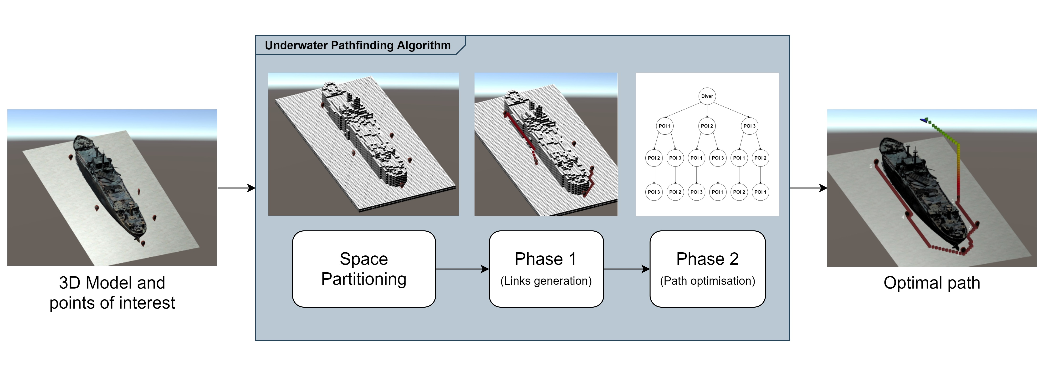
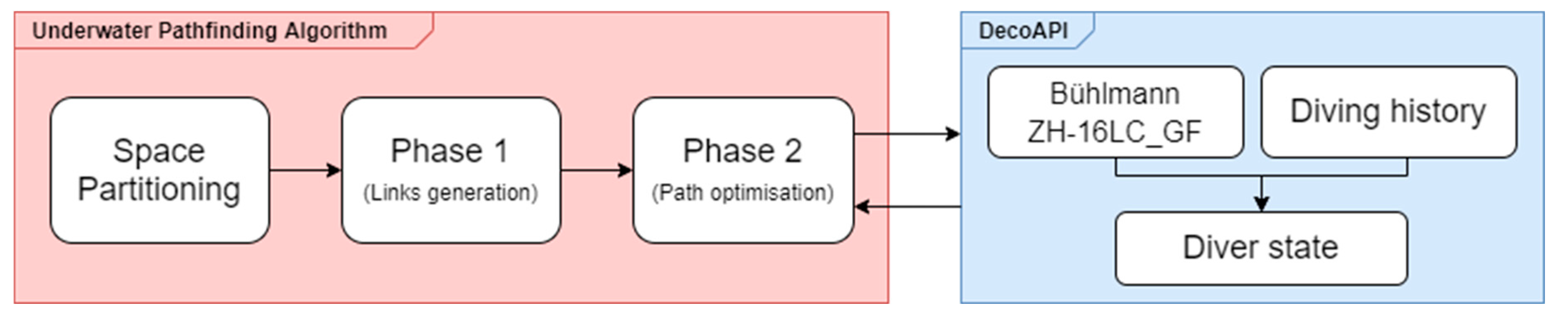
The proposed pathfinding algorithm is composed of different stages, each addressing a different problem. The first step is a preprocessing stage—namely, the space partitioning, in which the 3D model of the underwater environment is analysed and represented in a way that is simpler to be processed by a search algorithm. Subsequently, the process of searching the best path to visit a set of points of interest can be divided into two phases. In the first phase, all the best paths between each couple of POIs are generated (links generation). In the second phase, the best sequence to visit the major number of POIs is defined, aiming to minimise the cost of the visit (path optimisation). In both phases, the cost of the underwater movements was assessed with different strategies, where each of them determines the choice of a different best path. In order to take into account the aspects that are inherent to the underwater environment, in this last phase, the search algorithm relies on an external API (application programming interface)—namely, the DecoAPI, which records the history of the dive and evaluates the actual state of the diver parameters related to the dive. This API was developed separately from the pathfinding algorithm, and it implements the Bühlmann model ZH-16LC [21,22] extended with a gradient factor [23] to track and compute the decompression profile of the diver.
All stages of the pathfinding algorithm are represented in Figure 1 and described in more detail in the following sections.
2.1. Space Partitioning
The space partitioning is the process of dividing a space into nonoverlapping regions so that any point in the space can be associated with a single specific region. Representing a geometrical space in such a way can simplify different kinds of geometry queries, e.g., determining whether a ray intersects an object. Space partitioning is often used in 2D/3D path planning. In this case, the adjacent regions are connected to each other by modelling a graph, so the process of searching for the shortest path can be performed by the means of algorithms that operate in a graph.
For this purpose, it is very useful to divide the space into regions and to label the ones that correspond to the “water” and the ones matching the “terrain”, with the aim of discerning between the areas of the underwater site that the diver can pass through and the obstacles he/she has to avoid. In particular, the space is partitioned into voxels with shapes of equal size cubes (namely, one metre), forming a 3D grid. The exact dimension of the voxel was chosen in relation to the approximate dimension of a diver. Indeed, a voxel not bigger than the diver is enough to represent the underwater environment with sufficient accuracy. Even though it can produce a better approximation of the 3D map, a too-small voxel could be counterproductive. In fact, an undersized voxel could lead to paths that go through narrow passages where the diver should not and could not dive through. Moreover, it is worth noting that the size of the voxel directly affects the algorithm performance, because the smaller the voxel, the larger the total number of voxels that composes the 3D grid, and the computational cost of the search algorithm employed in phase 1 depends on the number of voxels involved in the search.
2.2. Phase 1 (Links Generation): Calculating Optimal Links between Pairs of POIs
In phase one, a graph was defined, where each node represents a “water” voxel of the 3D grid, i.e., a region that is accessible to the diver. Each voxel is connected to its neighbours, which are the adjacent voxels. The weight of the edges, connecting each node of the graph with its neighbours, depends on the strategy by which the cost of the underwater movements is defined. Given this graph, the problem that needs to be solved is the generation of the best paths between each couple of POIs. These best paths are referred to as “links”, because they represent the links of a second different graph that will be defined and used in phase 2. The best path between two given POIs is the one that minimises the defined cost, i.e., the shortest path. In graph theory, the shortest path problem requires to find a path between two nodes in a graph, so that the sum of the weight of the edges that belong to the path is minimised. In the literature, an algorithm that is widely used to solve this kind of a problem is A*, which is often used in many fields of computer science due to its completeness, optimality, and optimal efficiency [24]. A* is an informed search algorithm that uses a heuristic function to estimate the cost of the cheapest path from a given node to the goal node. The algorithm uses this information to focus its search toward a direction that most likely will lead to the optimal solution. The heuristic function is problem-specific, so it needs to be defined according to the context. If the heuristic function is admissible, meaning that it never overestimates the actual cost to reach the goal node, A* will always return a least-cost path from the starting node to the goal node.
As regards the weight of the edges of the graph, i.e., the cost of the underwater movements, three possible strategies were considered to define it: one based on the distance covered by the path, one on the air consumption, and the last on the decompression cost. Since the heuristic function is problem-specific, it is defined in a specific way for each strategy. These strategies are described in detail in the following subsections.
2.2.1. Distance
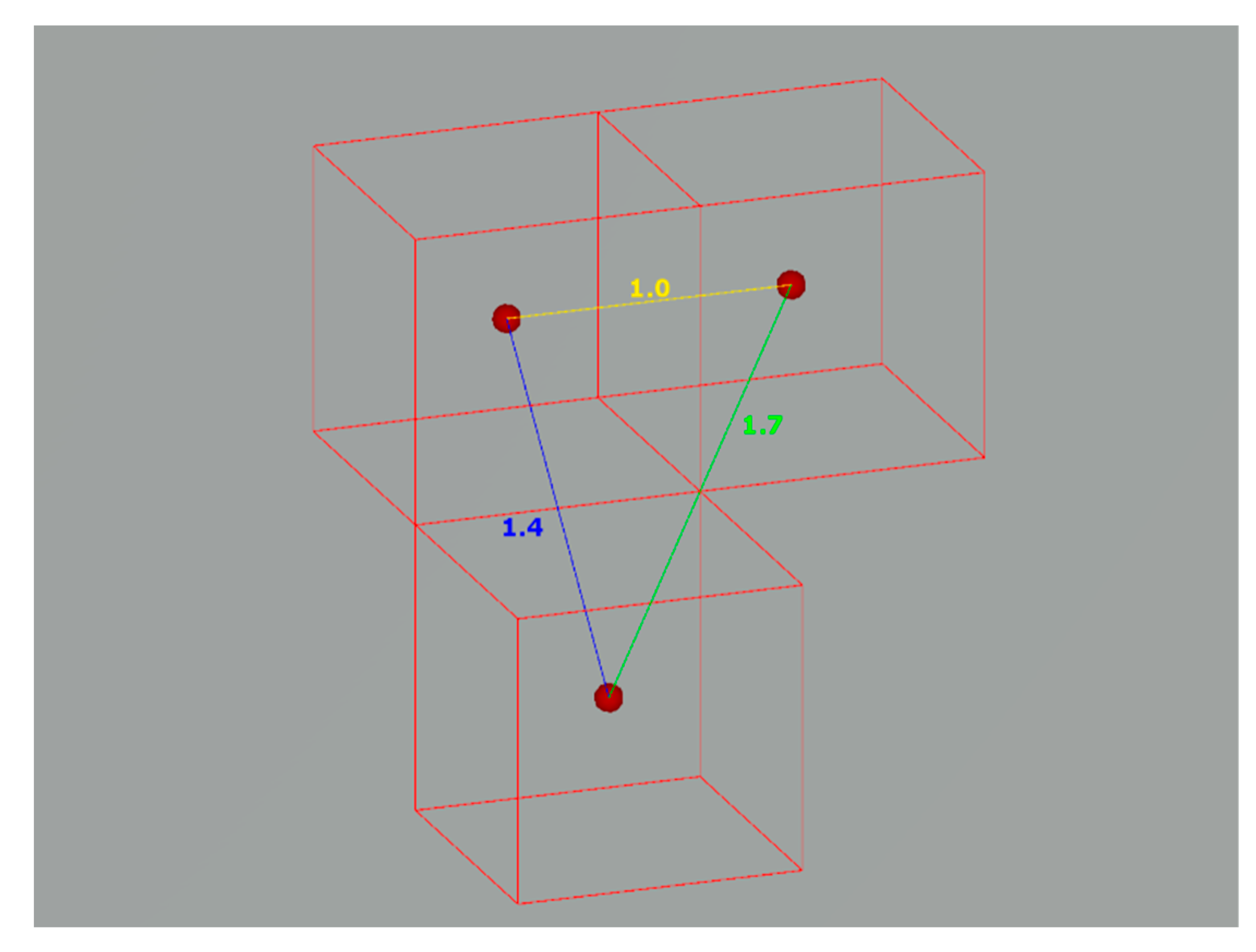
The simpler strategy is to consider the cost of an underwater path as the mere distance covered by the path. In the 3D grid, the allowable movements are restricted by the nature of the grid itself. Basically, three different types of movements are allowed in a 3D grid, and each of them has a different cost:
- Mov1D: It is the movement along only one axis. Given a voxel diameter of one meter, the cost of this kind of movement is defined as (Figure 2, yellow line).
- Mov2D: It is the movement along two axes. Its cost is defined as the diagonal of a square of a side equal to one: (Figure 2, blue line).
In this case, given two nodes, the heuristic function (1) is computed as the distance between the two nodes evaluated as movements in the 3D grid. Since the heuristic should not overestimate the distance, it is considered the best case, i.e., the minimum number of movements of a different kind that permits to reach one node from the other:
where is the number of movements for each type of movement.
2.2.2. Air Consumption
In an underwater environment, the covered distance is not the only factor to take into account while evaluating the cost of a path. Indeed, the diving depth is a factor that affects different aspects of the dive, such as the air consumption, the quantity of nitrogen absorbed, and, consequently, the need and the duration of the decompression stops at the end of diving. The air consumption depends both on the distance covered and the diving depth. Therefore, it could be a valid parameter to consider as a cost to be minimised.
To compute the air consumption, the respiratory minute volume (RMV) has to be considered as the air consumption rate [1]. The RMV is the total volume of air moved in and out of the lungs in one minute, and it is directly related to different exertion levels among divers. The air consumed at a given depth can be computed calculating the consumption rate at the depth with Equation (2):
where is expressed in scfm (standard cubic feet per minute), and is the absolute pressure (ata) at the given depth. Then, the air consumed (3) can be calculated by multiplying the by the travel time (min).
Given the distance of each type of movement, as described in the previous section, the travel time (4) can be defined as
where is the traveling speed that can be considered as a constant. Therefore, the cost (5) can be defined as
As is constant, i.e., it remains the same in the cost computation of whatever path, the cost function (5) can be simplified as follows (6):
On this basis, the heuristic function (7) can be defined, and it considers the best case of a path with the minimum distance, as computed in the previous section, and the minimum air consumption that matches the one evaluated on the surface ().
where is the number of movements for each type of movement, and the movement distances are the ones described in the previous section.
2.2.3. Decompression Cost
On the basis of the theory of the dissolved gas model of Bühlmann [21], it is possible to evaluate the partial pressure of inert gas dissolved in the tissue compartments of the diver. This pressure is an important parameter in the computation of decompression stops. In fact, the greater the pressure, the longer the time that will be eventually needed to complete safely the decompression.
Hence, the formulation of a “decompression cost” that is based on the inert gas pressure in the tissues and is computed by means of the Schreiner Equation (8) [25]:
- , compartment inert gas pressure (bar).
- , initial compartment inert gas pressure (bar).
- , initial inspired alveolar inert gas pressure (bar). = (, where is the initial ambient pressure, is the water vapour pressure at 37 degrees Celsius, i.e., 0.0627 bar, and is the fraction of inert gas.
- , half-time constant related to the compartment (min−1), .
- , time of exposure (min).
- , rate of change in inspired inert gas pressure with change in the ambient pressure (bar/min). , where is the rate of change in the ambient pressure, and is the fraction of inert gas.
In short, this equation evaluates the tissue inert gas pressure according to its initial state to the ambient pressure and to the ascent/descent rate. The idea is to define as the decompression cost, but in order to solve the concerning equation, some assumptions were necessary. It is assumed that the breathing mixture is atmospheric air, and therefore, the only inert gas considered is nitrogen. Typically, on the basis of the Bühlmann model, the equation is calculated for all 16 tissue compartments, but in this case, for the sake of simplicity, only the first compartment was considered, i.e., the one with the highest diffusion rate. This compartment has a half-time equal to 4 [22]. Furthermore, the time of exposure and the rate of change in inspired gas pressure are calculated assuming a speed of the diver equal to 10m/min. In addition, for the evaluation of , a fixed value stands for the fraction of nitrogen in the air. Finally, it was necessary to define the value of that is related to the diver initial state. Since the diver state is not known at this stage, it is assumed as a constant equal to the one computed on the surface before starting the dive. On the surface, the amount of nitrogen in the body is constant, so, in this case, the partial pressure of nitrogen (9) corresponds to the alveolar partial pressure:
On these bases, a table of the decompression costs was created. For each depth, three cases were considered: remaining at the same depth, ascending, and descending. For each of these cases, the cost of the three different movements allowed in the 3D grid were computed, as described previously. In Table 1, as a sample, only a part of the decompression cost table is reported.
As regards the heuristic function (10), similar to the other strategies, a path with the minimum distance and the minimum decompression cost that corresponds with the one evaluated on the surface was considered:
2.3. Phase 2 (Path Optimisation): Calculating Optimal Path to Visit All POIs
Once phase 1 is completed, all the best links through each couple of POIs have been computed. In phase two, a new graph with a node for each POI can be considered. This is a complete graph for which the links were computed in phase 1. Given this graph, the problem is to find the path that visits the highest possible number of POIs with the minimum cost. It is worth noting that it could be not possible to safely visit all the POIs. This is due to the constraint related to the diving safety procedures that take into account the remaining air in the tank and the absorption of nitrogen in the tissues that should not go beyond the limits. Taking into account all of these aspects, the search algorithm in this phase relies on the DecoAPI introduced before.
Therefore, the algorithm of phase 2 searches for the path that visits the highest possible number of POIs with the minimum cost and that is safe and feasible for the diver, given his/her actual state.
The cost of the path depends on the strategy employed in phase 1. In the case of strategies based on the distance and on the air consumption, the cost considered in phase 2 is the same as the one evaluated in phase 1, so each link of the new graph has a cost that matches the one computed for the related best link found in phase 1. In the other case of the strategy based on the decompression cost, the cost considered in phase 2 is based on a parameter evaluated by DecoAPI, i.e., the ascent pressure limit. It was decided to consider this cost during this phase, because it is directly related to the inert gas dissolved in the tissues on which the decompression cost of phase 1 is based as well. In particular, the ascent pressure limit stands for the minimum ambient pressure to which the diver can ascend without exceeding the critical supersaturation limit. Furthermore, the ascent pressure limit computed by DecoAPI can rely on the knowledge of the complete decompression profile of the diver, and, therefore, it is more realistic than the decompression cost computed in phase 1, which is based on some strong assumptions that could not correspond to the real case.
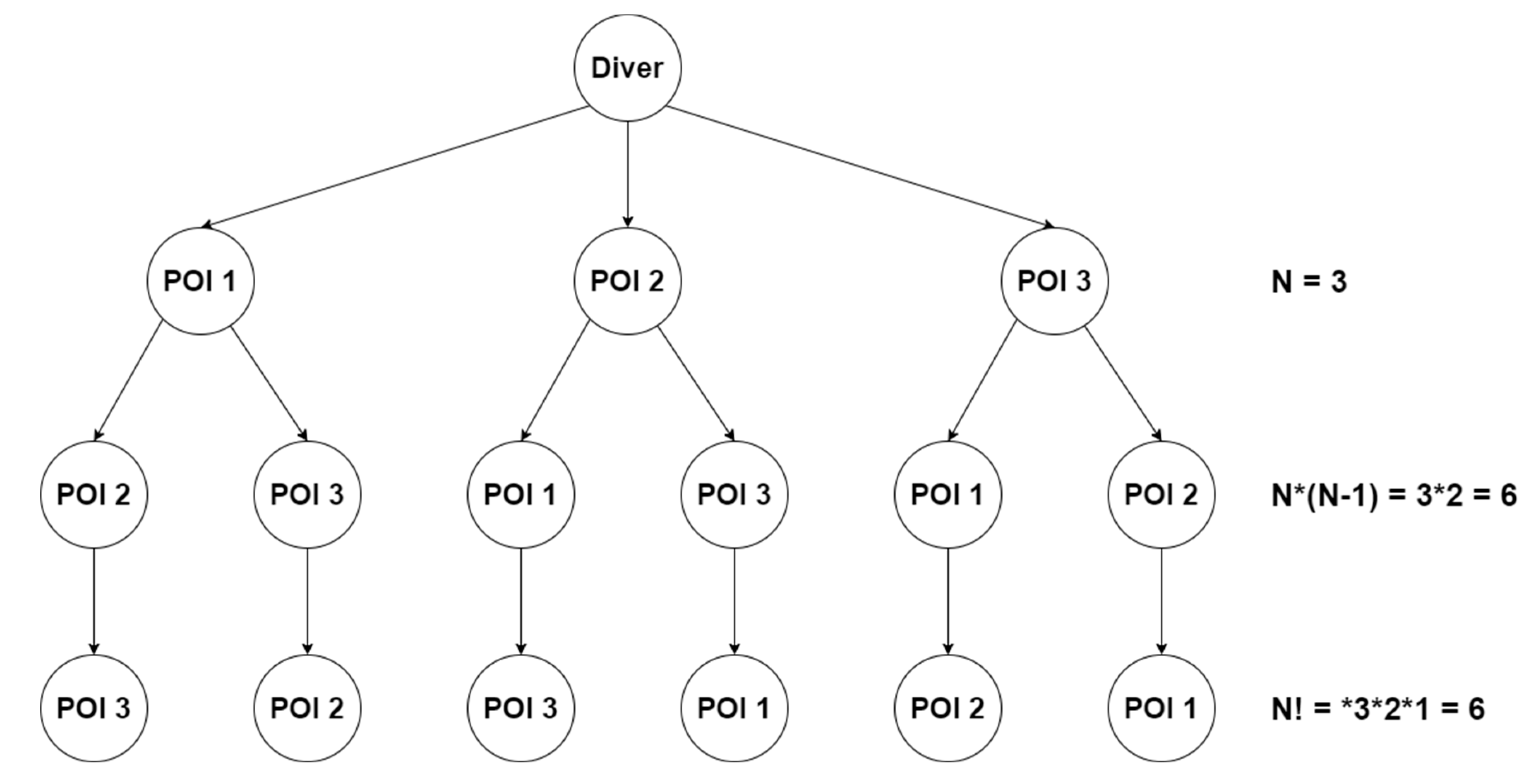
The space of the solutions can be represented as a tree (Figure 3). The root of the tree is represented by the diver, and the first level of the tree is composed of all the POIs. The child nodes of each branch node are all the POIs except the ones that are just present in the branch. The tree has a number of leaves that is , where N is the number of POIs. The number of the leaves corresponds to all possible paths that visit all the POIs. The total number of nodes of the tree (11) is given by the following formula:
that represents all the possible partial paths, i.e., the paths that visit only a subset of the given POIs.
A depth-first search algorithm for traversing the tree was implemented. As soon as it finds a path with a cost lower than the actual best path (if any), this is recorded as the best path. In addition, also, the best partial path is recorded, i.e., the path that visits the greater number of POIs with the lowest cost. If there is not a path that can visit all the existing POIs, this partial path will be returned as the best path. This is due to the fact that, apart from different strategies employed in phase 1, in phase 2, each eligible path is processed by DecoAPI and should result safe to be considered as a possible solution. A path is considered safe if the diver does not exceed the decompression limits and if he/she has enough time to fulfil the deco stops, thus concluding the dive in complete safety. DecoAPI performs this evaluation on the basis of the actual state of the diver. In fact, it records the dive profile of the diver in order to perform the estimation of the nitrogen absorbed by the tissues of the diver. When the tree is generated, the initial state of the diver corresponding to the root of the tree is recorded. At each branch node, the state of the diver is computed according to the actual path of the related branch and is propagated in the lowest level of the tree. This step avoids the repetition of expensive calculations that were previously done. Furthermore, a pruning of the search tree is implemented, i.e., a technique for the optimisation of the tree through the removal of the branches that are redundant in order to find the optimal solution. In particular, when a partial path has a cost that is greater than the cost of the actual minimal path, the related branch is deleted from the tree, and the search proceeds on to the next branch.
3. Results
The behaviour of the pathfinding algorithm was tested on each underwater site for each of the three strategies previously described. For each 3D model of the underwater sites, space partitioning was performed in order to produce a 3D grid on which the algorithm could perform the search of the best path.
3.1. Case Studies
Three cases of study were considered to evaluate the behaviour and the performance of the pathfinding algorithm. Each of them consisted of a 3D model that represented an underwater site with different environmental features. Five POIs were placed in each site, and they represented the spots that the diver needed to visit. The different environments are described in the following subsections.
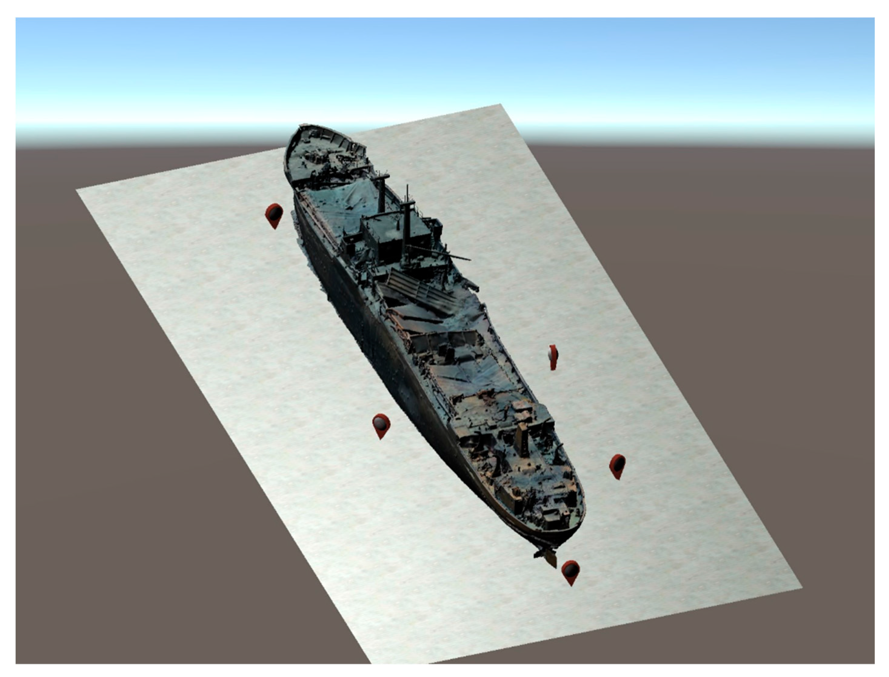
3.1.1. Shipwreck
This underwater site is a typical sample of an artificial obstacle in an underwater environment that could restrict the freedom of movement of the diver, and it has to be taken into account while computing a diving plan. In particular, in this case study, the obstacle is also the focus of the mission and is represented by a modern shipwreck that is 85 m long and approximately 13 m wide (Figure 4). The shipwreck lays on the seabed in an upright position at a depth of around 35 m. The deck of the ship is at a depth of around 30 m.
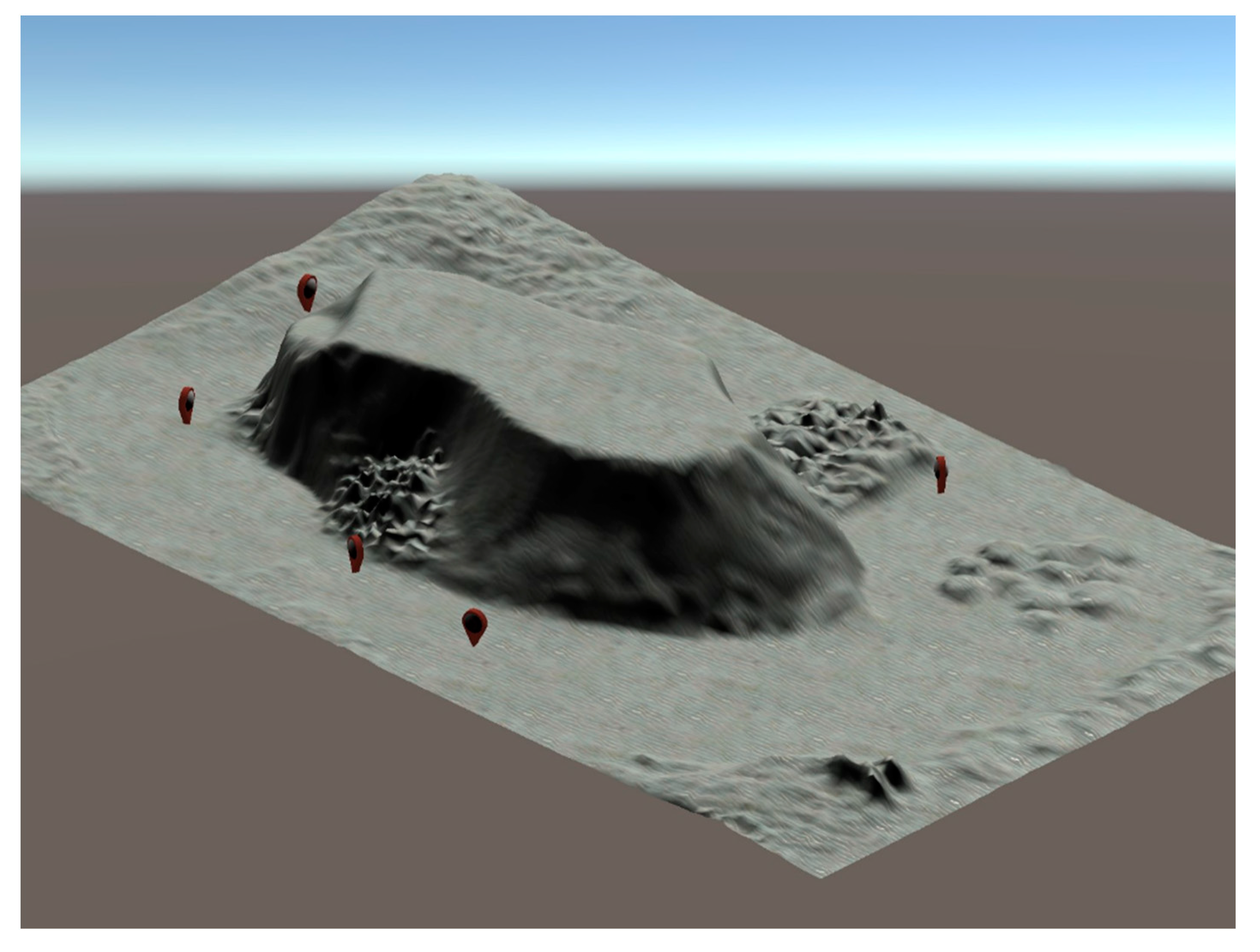
3.1.2. Seamount
This case study represents a sample of a natural obstacle in the underwater environment, such as a seamount (Figure 5). It is not a real environment but a 3D-modelled one. The depth at the seabed level is around 30 m, and the top of the seamount is 10 m deep.
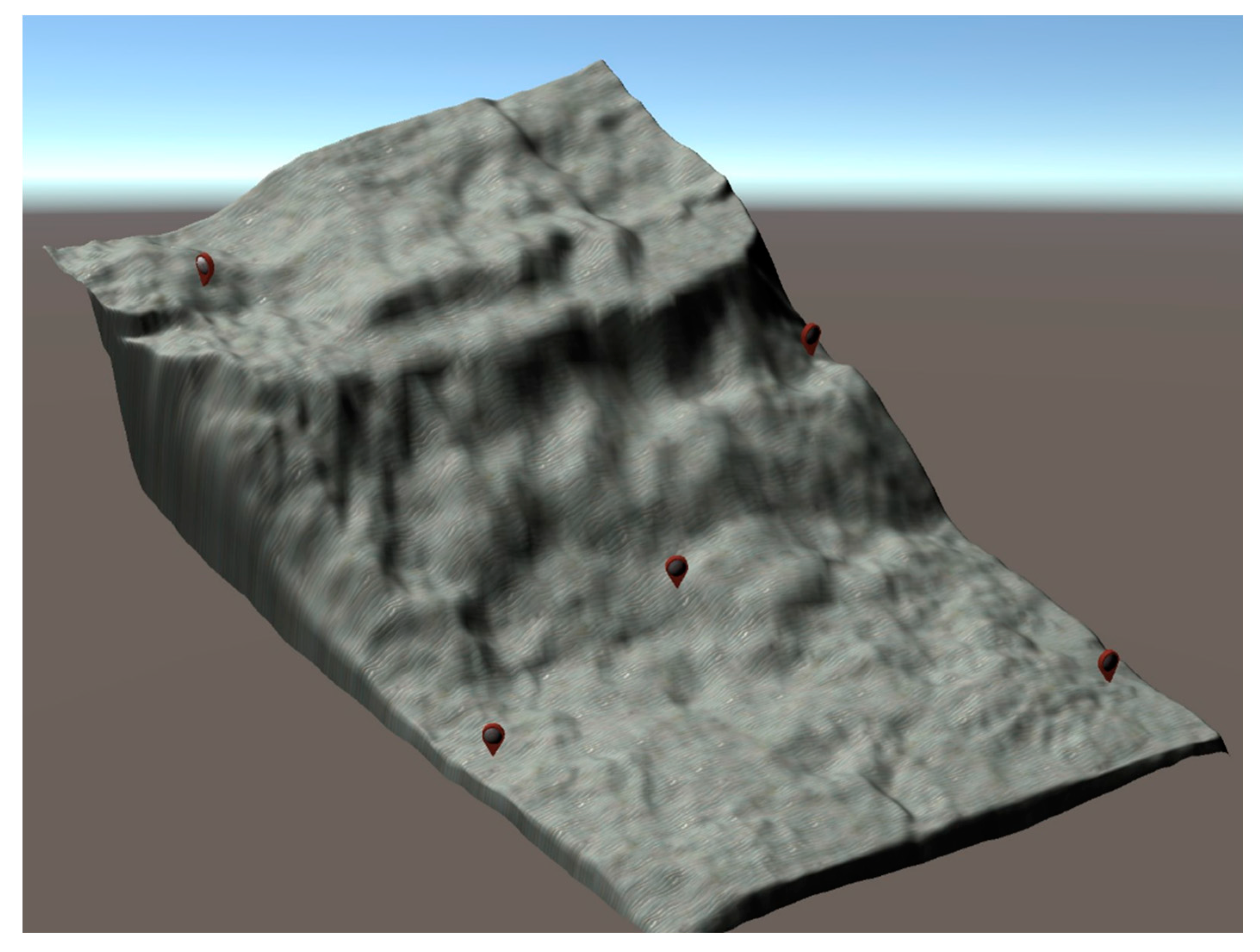
3.1.3. Landslide
A typical natural underwater formation is the landslide, i.e., an underwater slope where the depth increases gradually (Figure 6). In this case, the environment was modelled as well. The top region is around 7 to 8 m deep, and the bottom of the seabed is at a depth of around 27 m.
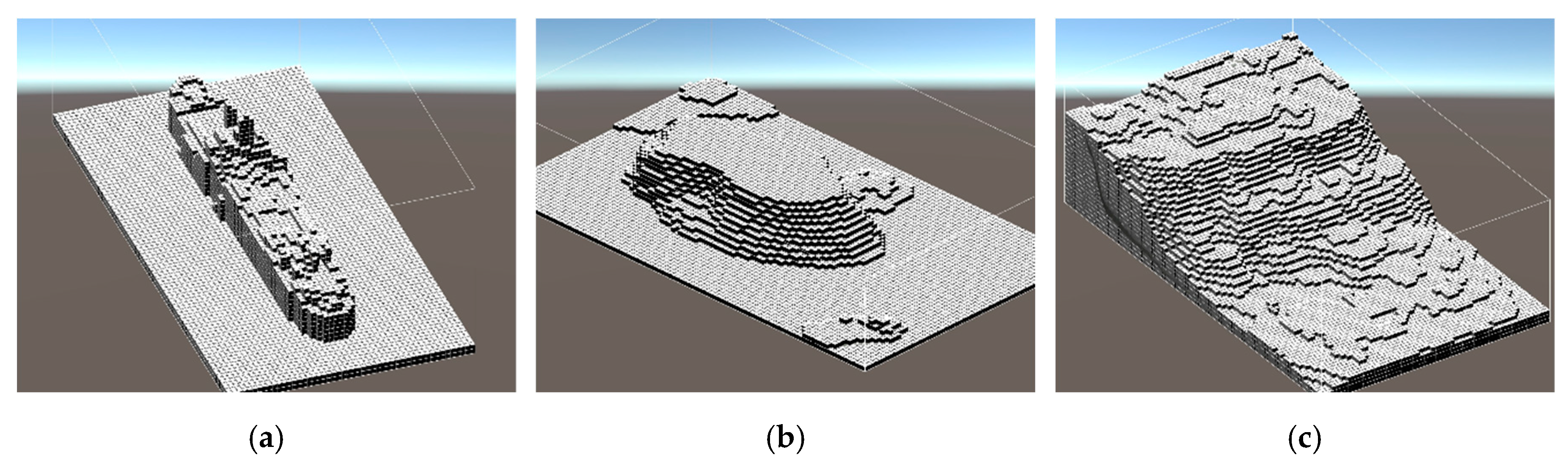
3.2. Space Partitioning: 3D Grids
Figure 7 represents the 3D grids for each case study. More precisely, the figure shows the voxels of the grids that represent the “terrain”, i.e., the regions of the underwater site that cannot be traversed by the diver, as described in the related section. The whole grid covers the entire underwater sites from the seabed to the surface. In the figure, the bounds of the grids are represented by the white lines.
3.3. Generated Paths
In Table 2, all generated paths are reported for each case. The rows represent the underwater sites, and the columns represent the strategy adopted to compute the related path. The position of the diver is set always on the surface, and the generated paths visit all the POIs in each case. The generated path is represented by the voxels of the grid that are part of the path. A gradient colour is used to better identify the depth of the path. The gradient ranges from the green colour on the surface to the red colour on the seabed. A numbered label near each POI indicates the order of visit.
For each path generated with a specific strategy, the costs of the other two strategies are also computed for the path. These costs are reported in Table 3, where each column represents the paths generated by the related strategy divided by the underwater site. Consequently, each row represents a specific type of cost. Within the row, the value highlighted in grey represents the minimum cost, and the value in bold represents the cost closest to the minimum.
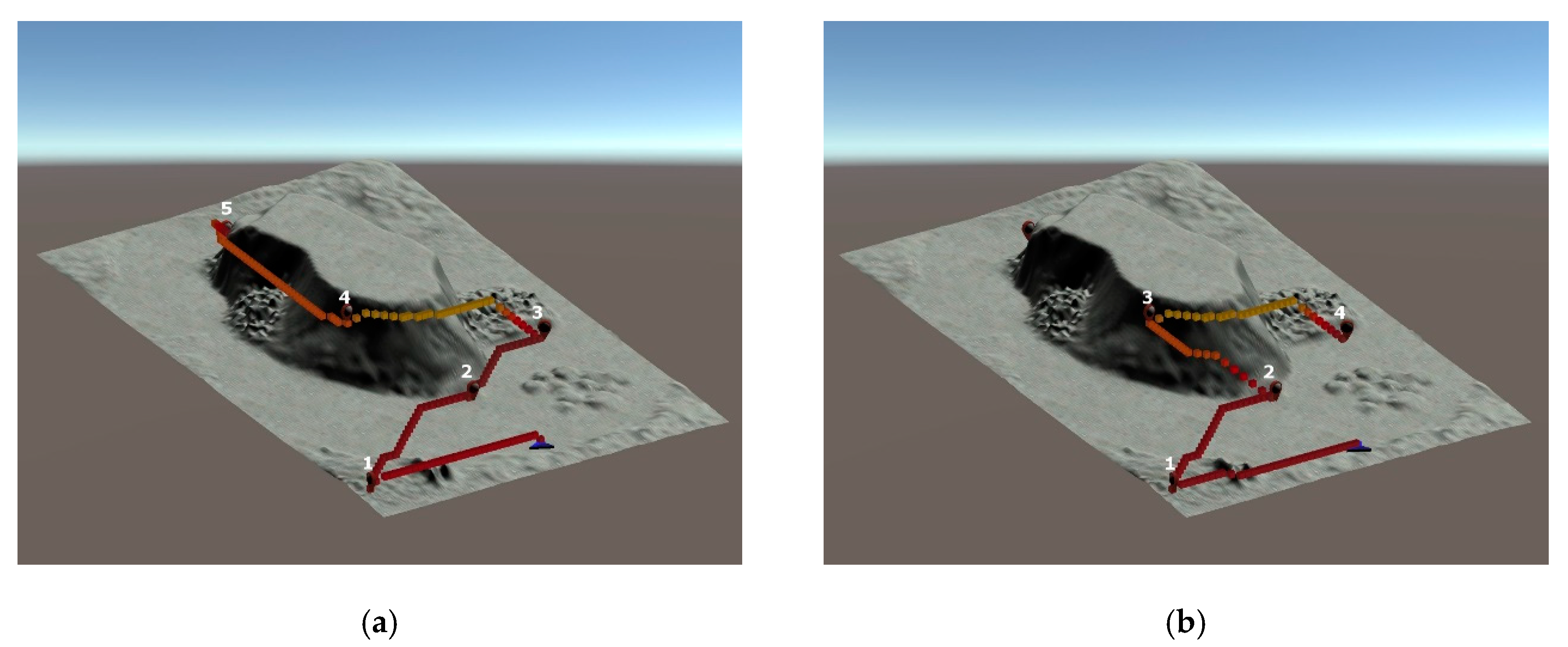
Over time, the paths determined by the pathfinding algorithm could change. In fact, the history of dives is recorded by DecoAPI, which evaluates the diving profile of the diver and establishes if a certain path is safe or not for the diver. Figure 8 and Table 4 depict two different moments of the same dive. In the first moment, the diver is diving at a depth of 18 m, and the related dive data are reported in the first column of Table 4, labelled as “Case a”. In this situation, the algorithm succeeds in finding a safe path to visit all the five POIs (Figure 8a). After fifteen minutes at the same depth of 18 m, the situation changes, as reported in the second column of Table 4, labelled as “Case b”. In fact, the ascent pressure limit, which meaning was defined before, increases from 0.97 to 1.64 bar. The air available in the tank goes down to 66 bar, and the time to surface (TTS) goes up to six minutes. In particular, the TTS is a typical diving concept that represents the time estimated for the diver to complete the eventual decompression stops and ascend safely to the surface. In this new situation, the pathfinding algorithm evaluates that it is no longer safe for the diver to visit all the five POIs. Therefore, it suggests an optimal partial path, i.e., a path that visits four POIs with the minimum cost and in complete safety.
4. Discussion
The results reported in Table 2 show that the algorithm behaves in a different way according to the adopted strategy. In particular, the strategy based on the distance produces a straightforward path that obviously takes into account only the distance covered by the path whilst ignoring the depth. On the contrary, the strategy that relies on the air consumption cost considers both the distance and the depth of the generated path. As a result, this strategy produces paths that suggest ascending a little in some cases, in order to dive at a lower depth and consume less air without impacting too much on the distance covered by the path. Finally, the strategy based on the decompression cost generates paths that suggest ascending more and more frequently with respect to the air consumption strategy. In addition, the strategy based on the decompression cost suggests visiting the POIs in an order that does not seem to be convenient or logical. This is due to the fact that this strategy does not take into account the distance covered by the path and suggests diving at lower depths as much as possible in order to minimise the ascent pressure limit. In fact, the ascent pressure limit is not an increasing function during the dive, but it can decrease while ascending. The costs reported in Table 3 allow for better addressing the differences between the results obtained by the alternative strategies. Obviously, each strategy obtains the best values (highlighted in grey) as regards the cost related to the strategy itself. The strategy based on the distance obtains an air consumption cost that is the closest to the minimum. The strategy based on air consumption seems to suggest paths that minimise the consumption of air, but, in addition, it obtains a distance cost and ascent pressure limit that are the closest to the minimum. On the contrary, the strategy based on the decompression cost seems successful only in optimising the ascent pressure limit while suggesting paths that have a distance and air consumption cost that are considerably higher with respect to the other two strategies.
Each strategy may consider or not the diving depth and, eventually, can suggest paths with an ascent of a variable entity before moving towards the target. In this respect, Table 5 reports some figures that address the different behaviours of strategies in suggesting the entity of the ascent. Each figure shows the paths suggested by each strategy that goes from the diver to a POI placed at a given distance and depth. At a depth of 10 m and a distance of 10 m, all the three strategies suggest moving straightforward, maintaining the depth. Increasing the distance to 20 m, the air consumption (AC) strategy suggests ascending a few meters, and the decompression strategy suggests ascending even more. With a distance of 30 m, both strategies suggest ascending up to the surface. Obviously, the strategy based on the distance does not ever suggest ascending, because it does not consider depth as a cost. Going deeper, to 20 m, with the POI placed at a distance of 10 m, the three strategies continue to suggest remaining the same depth. At a distance of 20 m, the only strategy that suggests ascending a few meters is the one based on the decompression cost. A further increasing of the distance of the POI up to 30 m leads the AC strategy to suggest ascending about five meters, while the strategy based on the decompression cost suggests ascending about 10 m. It is worth noting that, basically, the AC strategy suggests ascending less with respect to the decompression strategy, placing itself in the middle between the other two strategies.
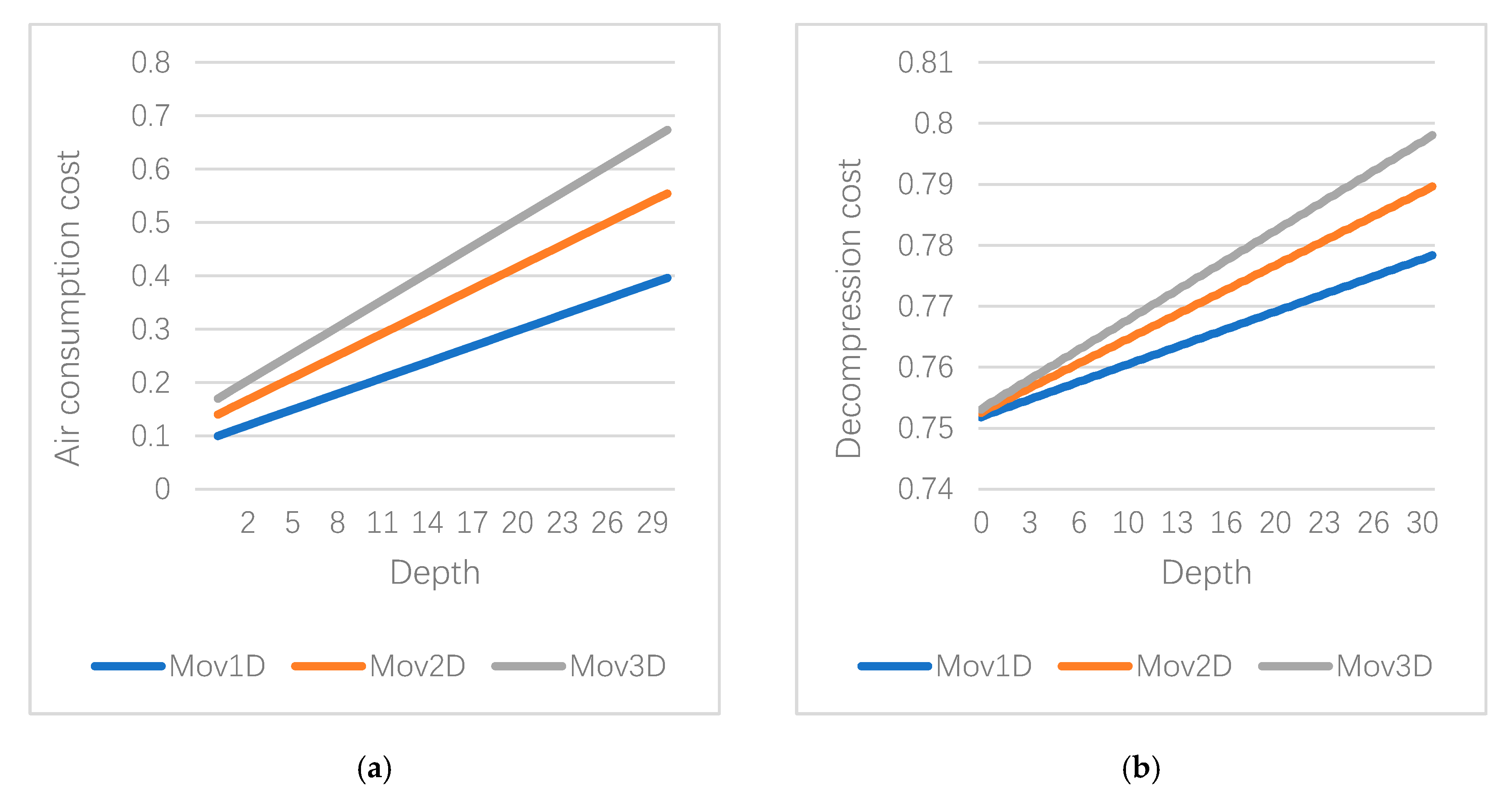
In addition, it could be noted that both the AC and decompression strategies suggest ascending less with the increase of the depth. This could be explained by observing the graphs in Figure 9. In both graphs, each line represents the evolution of the different types of movements with the increase of the depth. It could be noticed that the slope of each line is different. Consequently, as the depth increases, the gap between different types of movement increases as well. This shows that it is less affordable to extend the path ascending with diagonal movements.
Finally, it has to be noted that, in the results reported, the strategies could also decide to ascend up to the surface without any constraint in order to evaluate the pure behaviour of the strategy. In a real case, it is convenient to introduce an ascent limit that can prevent the strategies from ascending too much. Indeed, the possibility to enable this limit was introduced in the pathfinding algorithm, and it was set at the depth of the safety decompression stop, which, usually, is at five meters and has to be completed at the end of every dive.
5. Conclusions
In this work, a novel system was presented that enabled computing an underwater path that visits the highest possible number of POIs with the minimum cost and in total safety. This was achieved by designing an original pathfinding algorithm that took into account several factors strictly inherent to scuba diving. In fact, the algorithm took into account the decompression limits and the remaining air in the scuba tank. Furthermore, for the first time in the field of path planning aimed to support divers, the proposed system took into account the topography of the underwater environment to produce a path that considered and avoided obstacles.
The pathfinding algorithm computes the path with the minimal cost. In order to define the cost of the underwater movements, three possible strategies are considered: the first one based on the distance covered by the path, the second on the air consumption, and the last one on the decompression cost.
The analysis of the results suggests that the best strategy is the one based on the optimisation of the air consumption. The decompression cost is based on the ascent pressure limit that takes into account only nitrogen absorbed in the tissues. For this reason, the strategy based on this cost tends to suggest paths that ascend too much towards the surface, without taking into consideration the additional distance of the path. Conversely, the strategy based only on the distance cost does not consider the depth of the path and optimises only the length of the path. In the middle, between these two strategies, the strategy based on air consumption takes into account both the distance and the depth, minimising the diving at great depths without affecting too much the path’s length. Furthermore, since the AC strategy tends to ascend less than the strategy based on the decompression cost; it suggests paths that are more plausible and relevant to the standard scuba diving practices. An ascent limit that can prevent the strategies from ascending too much was designed as well.
In the future, it will be necessary to evaluate additional strategies or to combine the existing ones in a different fashion. Indeed, it could be possible to adopt different strategies for the evaluation of the costs in the two different phases of the algorithm. Some field tests will be conducted with real users that could give important feedback to evaluate which strategy could perform better in a real case scenario. In addition, since divers often return to known locations at the end of the dive (i.e., the boat), a fixed final node in the computation of the best path could be introduced. This will strongly change the generated paths and may ensure a better suiting of real diving demands. Finally, a further extension could also take into account the sea currents that may affect considerably the cost of a specific path.
Author Contributions
Conceptualisation, M.M. and F.B.; methodology, M.M., F.B., and F.P.; software, M.M.; validation, M.M., F.P., and A.C.; writing—original draft preparation, M.M.; writing—review and editing, M.M., F.B., F.P., and A.C.; supervision, F.B.; funding acquisition, F.B. All authors have read and agreed to the published version of the manuscript.
Funding
This research was partially funded by the Regione Calabria under the POR CALABRIA FESR-FSE 2014-2020 as part of the MOLUX (MObile Lab for Underwater eXploration) project (CUP J28C17000110006).
Conflicts of Interest
The authors declare no conflict of interest.
References
- Joiner, J.T. NOAA Diving Manual: Diving for Science and Technology, 4th ed.; Best Publishing Company: Flagstaff, AZ, USA, 2001; ISBN 9780941332705. [Google Scholar]
- MultiDeco VPM & VPM-B & VPM-B/E & ZHL GF Dive Decompression Software for Technical Divers. Available online: http://www.hhssoftware.com/multideco/ (accessed on 31 August 2020).
- Subsurface | An Open Source Divelog. Available online: https://subsurface-divelog.org/it/ (accessed on 31 August 2020).
- DIVEROID. Available online: https://app.diveroid.com/en/main (accessed on 31 August 2020).
- DecoTengu-Dive Decompression Library. Available online: https://wrobell.dcmod.org/decotengu/ (accessed on 31 August 2020).
- Choset, H.M.; Hutchinson, S.; Lynch, K.M.; Kantor, G.; Burgard, W.; Kavraki, L.E.; Thrun, S.; Arkin, R.C. Principles of Robot Motion: Theory, Algorithms, and Implementation; MIT Press: Cambridge, MA, USA, 2005; ISBN 9780262033275. [Google Scholar]
- Murphy, R.R. Introduction to AI Robotics. Ind. Robot Int. J. 2001, 28, 266–267. [Google Scholar] [CrossRef] [Green Version]
- Dijkstra, E.W. A note on two problems in connexion with graphs. Numer. Math. 1959, 1, 269–271. [Google Scholar] [CrossRef] [Green Version]
- Hart, P.E.; Nilsson, N.J.; Raphael, B. A formal basis for the heuristic determination of minimum cost paths. IEEE Trans. Syst. Sci. Cybern. 1968, 4, 100–107. [Google Scholar] [CrossRef]
- Yang, J.-M.; Tseng, C.-M.; Tseng, P.S. Path planning on satellite images for unmanned surface vehicles. Int. J. Nav. Archit. Ocean Eng. 2015, 7, 87–99. [Google Scholar] [CrossRef] [Green Version]
- Sun, Y.; Ran, X.; Zhang, G.; Xu, H.; Wang, X. AUV 3D Path Planning Based on the Improved Hierarchical Deep Q Network. J. Mar. Sci. Eng. 2020, 8, 145. [Google Scholar] [CrossRef] [Green Version]
- Pham, H.X.; La, H.M.; Feil-Seifer, D.; Nguyen, L.V. Autonomous uav navigation using reinforcement learning. arXiv 2018, arXiv:1801.05086. [Google Scholar]
- Wang, C.; Wang, J.; Wang, J.; Zhang, X. Deep Reinforcement Learning-based Autonomous UAV Navigation with Sparse Rewards. IEEE Internet Things J. 2020, 7, 6180–6190. [Google Scholar] [CrossRef]
- Wang, X.; Yao, X.; Zhang, L. Path Planning under Constraints and Path Following Control of Autonomous Underwater Vehicle with Dynamical Uncertainties and Wave Disturbances. J. Intell. Robot. Syst. 2020, 99, 891–908. [Google Scholar] [CrossRef]
- Kulkarni, C.S.; Lermusiaux, P.F.J. Three-dimensional time-optimal path planning in the ocean. Ocean Model. 2020, 152, 101644. [Google Scholar] [CrossRef]
- Koenig, S.; Likhachev, M.; Furcy, D. Lifelong planning A∗. Artif. Intell. 2004, 155, 93–146. [Google Scholar] [CrossRef] [Green Version]
- Miskovic, N.; Nad, D.; Rendulic, I. Tracking divers: An autonomous marine surface vehicle to increase diver safety. IEEE Robot. Autom. Mag. 2015, 22, 72–84. [Google Scholar] [CrossRef]
- Bruno, F.; Lagudi, A.; Muzzupappa, M.; Lupia, M.; Cario, G.; Barbieri, L.; Passaro, S.; Saggiomo, R. Project VISAS: Virtual and Augmented Exploitation of Submerged Archaeological Sites-Overview and First Results. Mar. Technol. Soc. J. 2016, 50, 119–129. [Google Scholar] [CrossRef]
- Zingaretti, S.; Scaradozzi, D.; Ciuccoli, N.; Costa, D.; Palmieri, G.; Bruno, F.; Ritacco, G.; Cozza, M.; Raxis, P.; Tzifopanopoulos, T.; et al. A Complete IoT Infrastructure to Ensure Responsible, Effective and Efficient Execution of Field Survey, Documentation and Preservation of Archaeological Sites. In Proceedings of the 2018 IEEE 4th International Forum on Research and Technology for Society and Industry (RTSI), Palermo, Italy, 10 September 2018; pp. 1–6. [Google Scholar]
- Bruno, F.; Barbieri, L.; Mangeruga, M.; Cozza, M.; Lagudi, A.; Čejka, J.; Liarokapis, F.; Skarlatos, D. Underwater augmented reality for improving the diving experience in submerged archaeological sites. Ocean Eng. 2019, 190, 106487. [Google Scholar] [CrossRef]
- Bühlmann, A.A. Decompression—Decompression Sickness; Springer Science & Business Media: Berlin, Germany, 2013; ISBN 9783662024096. [Google Scholar]
- Bühlmann, A.A.; Völlm, E.B.; Nussberger, P. Tauchmedizin: Barotrauma Gasembolie—Dekompression Dekompressionskrankheit Dekompressionscomputer; Springer: Berlin, Germany, 2013; ISBN 9783642559396. [Google Scholar]
- Baker, E.C. Understanding M-values. Immersed 1998, 3, 23–27. [Google Scholar]
- Brewka, G. Artificial intelligence—A modern approach by Stuart Russell and Peter Norvig, Prentice Hall. Series in Artificial Intelligence, Englewood Cliffs, NJ. Knowl. Eng. Rev. 1996, 11, 78–79. [Google Scholar] [CrossRef]
- Schreiner, H.R.; Kelley, P.L. A Pragmatic View of Decompression. In Underwater Physiology; Lambertsen, C.J., Ed.; Academic Press: Cambridge, MA, USA, 1971; pp. 205–219. ISBN 9780124347502. [Google Scholar]
Figure 1.
The stages of the pathfinding algorithm and communication with DecoAPI.

Figure 2.
A representation of the three different types of movements allowed in a 3D grid with the related distance costs.
Figure 2.
A representation of the three different types of movements allowed in a 3D grid with the related distance costs.

Figure 3.
The search tree in the sample case of three points of interest (POIs).

Figure 4.
A modern shipwreck.

Figure 5.
A sample of a seamount.

Figure 6.
A sample of a landslide.

Figure 7.
The 3D grids of each underwater site: (a) the shipwreck, (b) the seamount, and (c) the landslide.
Figure 7.
The 3D grids of each underwater site: (a) the shipwreck, (b) the seamount, and (c) the landslide.

Figure 8.
The path suggested by the algorithm changes over time.

Figure 9.
The evolution of the air consumption cost (a) and the decompression cost (b) with the increasing of the depth.
Figure 9.
The evolution of the air consumption cost (a) and the decompression cost (b) with the increasing of the depth.


Table 1.
A part of the decompression cost table.
| Depth | Direction | Mov1D | Mov2D | Mov3D | P_alv0 |
|---|---|---|---|---|---|
| 0 | Same | 0.752156728 | 0.753014201 | 0.753655358 | 1 |
| 0 | Down | 0.752493664 | 0.753485367 | 0.754226993 | 1 |
| 1 | Up | 0.752682484 | 0.753748715 | 0.754545865 | 1.1 |
| 1 | Same | 0.753019419 | 0.754219881 | 0.755117501 | 1.1 |
| 1 | Down | 0.753356355 | 0.754691047 | 0.755689137 | 1.1 |
| 2 | Up | 0.753545175 | 0.754954395 | 0.756008008 | 1.2 |
| 2 | Same | 0.753882111 | 0.755425561 | 0.756579644 | 1.2 |
| 2 | Down | 0.754219046 | 0.755896727 | 0.75715128 | 1.2 |
| 3 | Up | 0.754407866 | 0.756160076 | 0.757470151 | 1.3 |
| 3 | Same | 0.754744802 | 0.756631242 | 0.758041787 | 1.3 |
| 3 | Down | 0.755081737 | 0.757102408 | 0.758613423 | 1.3 |
| 4 | Up | 0.755270558 | 0.757365756 | 0.758932294 | 1.4 |
| 4 | Same | 0.755607493 | 0.757836922 | 0.75950393 | 1.4 |
| 4 | Down | 0.755944429 | 0.758308088 | 0.760075566 | 1.4 |
| 5 | Up | 0.756133249 | 0.758571436 | 0.760394438 | 1.5 |
| 5 | Same | 0.756470184 | 0.759042602 | 0.760966073 | 1.5 |
| 5 | Down | 0.75680712 | 0.759513768 | 0.761537709 | 1.5 |
Table 2.
The paths generated with three different strategies for three different case studies.
| Underwater Site | Strategy | ||
|---|---|---|---|
| Distance | Air Consumption | Decompression | |
| Shipwreck |  |  |  |
| Seamount |  |  |  |
| Landslide |  |  |  |
Table 3.
The costs computed for each path with the tree strategy.
| Underwater Site | Cost | Strategy | ||
|---|---|---|---|---|
| Distance | Air Consumption | Decompression | ||
| Shipwreck | Distance | 167 | 172.2 | 301.7 |
| Air Consumption | 13.5292 | 13.4948 | 20.6618 | |
| Decompression | 2.277739 | 2.14631 | 0.8656095 | |
| Seamount | Distance | 139.2 | 143.5 | 175.6 |
| Air Consumption | 8.3121 | 8.2405 | 9.3926 | |
| Decompression | 0.5507061 | 0.548093 | 0.5466153 | |
| Landslide | Distance | 223.7 | 227.4 | 292.4 |
| Air Consumption | 12.1802 | 11.7076 | 13.9602 | |
| Decompression | 0.5526806 | 0.548951 | 0.5451685 | |
Table 4.
The dive data associated with the two cases presented in Figure 8.
Table 4.
The dive data associated with the two cases presented in Figure 8.
| Dive Data | Initial State | |
|---|---|---|
| Case “a” | Case “b” | |
| Time (min) | 39 | 54 |
| Diving depth (m) | 18 | 18 |
| Ascent pressure limit (bar) | 0.97 | 1.64 |
| Tank (bar) | 95 | 66 |
| Time to Surface (min) | 2 | 6 |
Table 5.
Different behaviours of the strategies in suggesting the ascent by varying the depth and the distance between the diver and point of interest (POI).
Table 5.
Different behaviours of the strategies in suggesting the ascent by varying the depth and the distance between the diver and point of interest (POI).
| Depth | Distance between Diver and POI | ||
|---|---|---|---|
| 10 m | 20 m | 30 m | |
| 10 m |  |  |  |
| 20 m |  |  |  |
Publisher’s Note: MDPI stays neutral with regard to jurisdictional claims in published maps and institutional affiliations. |
© 2020 by the authors. Licensee MDPI, Basel, Switzerland. This article is an open access article distributed under the terms and conditions of the Creative Commons Attribution (CC BY) license (http://creativecommons.org/licenses/by/4.0/).
Share and Cite
MDPI and ACS Style
Mangeruga, M.; Casavola, A.; Pupo, F.; Bruno, F. An Underwater Pathfinding Algorithm for Optimised Planning of Survey Dives. Remote Sens. 2020, 12, 3974. https://doi.org/10.3390/rs12233974
AMA Style
Mangeruga M, Casavola A, Pupo F, Bruno F. An Underwater Pathfinding Algorithm for Optimised Planning of Survey Dives. Remote Sensing. 2020; 12(23):3974. https://doi.org/10.3390/rs12233974
Chicago/Turabian StyleMangeruga, Marino, Alessandro Casavola, Francesco Pupo, and Fabio Bruno. 2020. "An Underwater Pathfinding Algorithm for Optimised Planning of Survey Dives" Remote Sensing 12, no. 23: 3974. https://doi.org/10.3390/rs12233974
Note that from the first issue of 2016, this journal uses article numbers instead of page numbers. See further details here.