Surface Motion Prediction and Mapping for Road Infrastructures Management by PS-InSAR Measurements and Machine Learning Algorithms


Abstract
:
1. Introduction
- An extensive literature review has been conducted in all sections of the paper by adding 120 references;
- This study proposes a prediction of surface motion rate for an extended area (from 132 km2 to 964 km2);
- A wrapper feature selection approach has been introduced in order to reduce the computational complexity of the algorithms, improving their interpretability, reduce overfitting issues, and also increase the overall predictive performance. Our previous study did not include this preprocessing step;
- Only PS observations have been used as target output to be modeled. Conversely, in Reference [2], we considered as output an interpolated map of PS-InSAR measures realized by the Inverse Distance Weighting process. Therefore, in this paper, we deal with real observation, avoiding the hypothesis that the measurements are correlated with each other through a predetermined distance function;
- In this paper, we not only used Regression Tree (RT) algorithm that was used in Reference [2] but also investigated three MLAs, namely Support Vector Machine (SVM), Random Forest (RF), and Boosted Regression Trees (BRT);
- Bayesian Optimization Algorithm (BOA) and 10-Fold Cross-Validation (CV) have been implemented to ensure that the best set of hyperparameters has been found out automatically. Therefore, we avoided to use of manual, random, or grid searches (that require user experience and a higher computational cost);
- The Taylor Diagram and scatterplots have been computed to evaluate and compare the algorithms appropriately (in addition to R2, Root Mean Square Error (RMSE), and Mean Absolute Error (MAE));
- Once the surface motion maps have been computed, we propose two additional case studies (i.e., two critical road sites) for evaluating the reliability of the suggested methodology.
2. Related Works
2.1. InSAR Techniques and InSAR for Road Monitoring and Inspection
- planning, where the PS-InSAR technique is implemented for identifying areas where building new infrastructures [36];
- prevention, where PS-InSAR is used to provide maintenance plans relying on the magnitude of the detected surface motion [37];
- monitoring and inspection, an interferometric process is used to detect critical infrastructural damages, identifying sections in which there are substantial movements [38]. We found researches on the implementation of PS-InSAR for road infrastructures [36,37,38,39,40,41,42], rail infrastructures [29,43,44,45,46], bridges [47,48,49,50], and dams [51,52,53,54];
2.2. Environmental Modeling by Machine Learning Modeling
- Most of the studies involve the prediction of landslides, probably because they are the phenomenon that is most manifested worldwide. Some other relevant topics are flood susceptibility, gully erosion by stream power, and groundwater potential mapping. Subsidence, settlements, uplift, and, in general, surface motion prediction seems to have a lower interest from the academic community. However, the losses caused by these effects can still be enormous, and it is essential to be able to predict and mitigate their effects;
- Most of the study involves a classification approach, i.e., the MLAs are calibrated for providing a binary output; thus, they can predict the presence or the absence of the phenomena, but nothing can be said regarding the intensity, the duration, and the direction. Conversely, Regression approaches attempt to predict a numerical output, i.e., they can provide information regarding a parameter of interest of a phenomenon (e.g., the safety factor in slope stability assessment or the settlement ratio in subsidence modeling). They suppose that a phenomenon could manifest over the entire study area;
- An extensive set of implemented MLAs has been identified. There are numerous studies in which the algorithms are single learners (such as Classification and Regression Tree (CART) or SVM), and several ones in which ensemble learners are adopted (through aggregation techniques, such as bagging or boosting). Generally, they belong to three families: tree-based models (e.g., CART, RF, and BRT), Artificial Neural Network (ANN)-based models, and SVM-based models. Other algorithms often used are Logistic Regression (LR), Frequency Ratio (FR) (they only work for classification tasks), and Multivariate Adaptive Regression Splines (MARS). Other types of algorithms, less used, are shown in Table 1;
- The metrics for evaluating the performance of MLAs are also manifold. The vast majority of classification-based studies present the calculation of the Area Under the Receiver Operating Characteristic (AUROC) and Accuracy. In regression-based studies, the most common parameters are the R2, RMSE, and MAE;
- A feature selection approach before the training phase is not always implemented. Indeed, in about half of the reviewed papers, the authors declare that the set of conditioning factors is defined relying on expert judgment or their previous implementation in other papers, or simply describe the set of parameters without precise justifications. It must be said, however, that the set of conditioning factors are often the same for all the reviewed studies.
- When a feature selection approach is implemented, the computation of the Variance Inflation Factors (VIF) has often been found. This parameter tests the multicollinearity of the factors, excluding the redundant ones. Unfortunately, VIF can only consider linear relationships between features, and in complex phenomena, this hypothesis appears strong. However, the VIF proposes a simple calculation, and the experience demonstrated by its extensive use shows that it still has a beneficial effect on modeling. Sometimes authors decide to test different subsets of features (for example, using a set with few features and a set with many of them) and compare the performance of MLAs. This technique could be useful for identifying a good subset of features excluding the less relevant ones, but if the subdivision into different datasets does not follow a specific algorithm, a satisfactory result is not guaranteed. More sophisticated feature selection methods, such as Principal Component Analysis (PCA) or Wrapper approaches, have been identified in limited research. Although they are powerful techniques, their limited use could derive from the excessive computational cost required.
3. Methodology
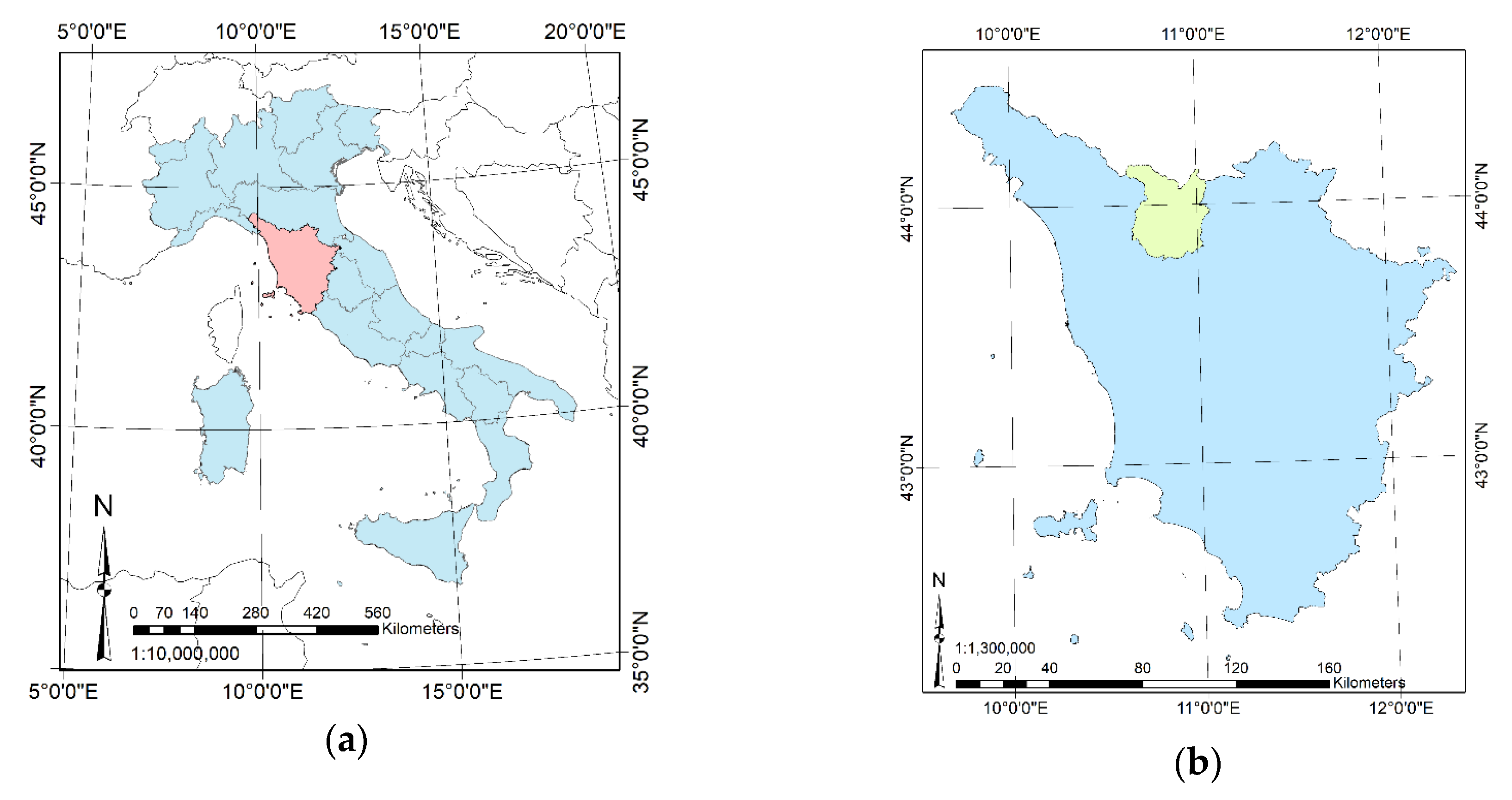
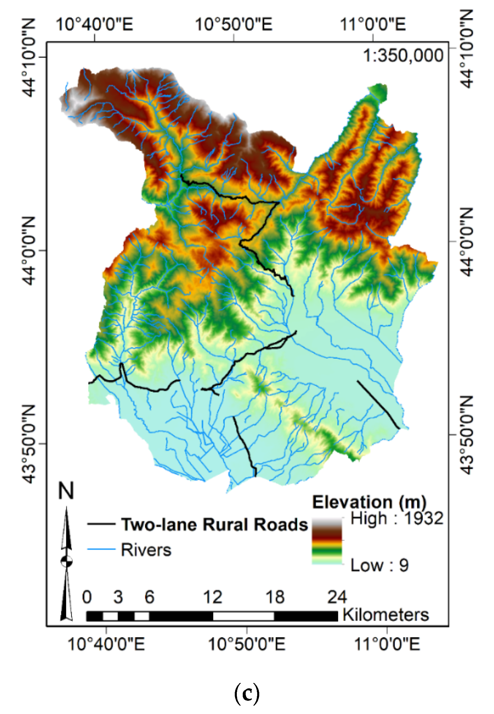
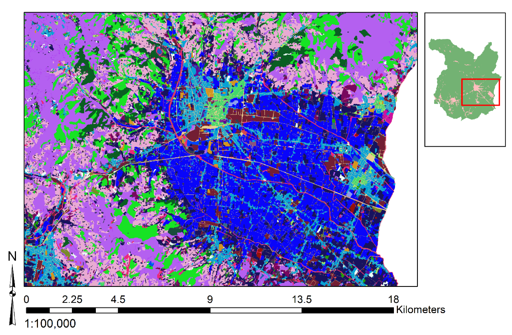
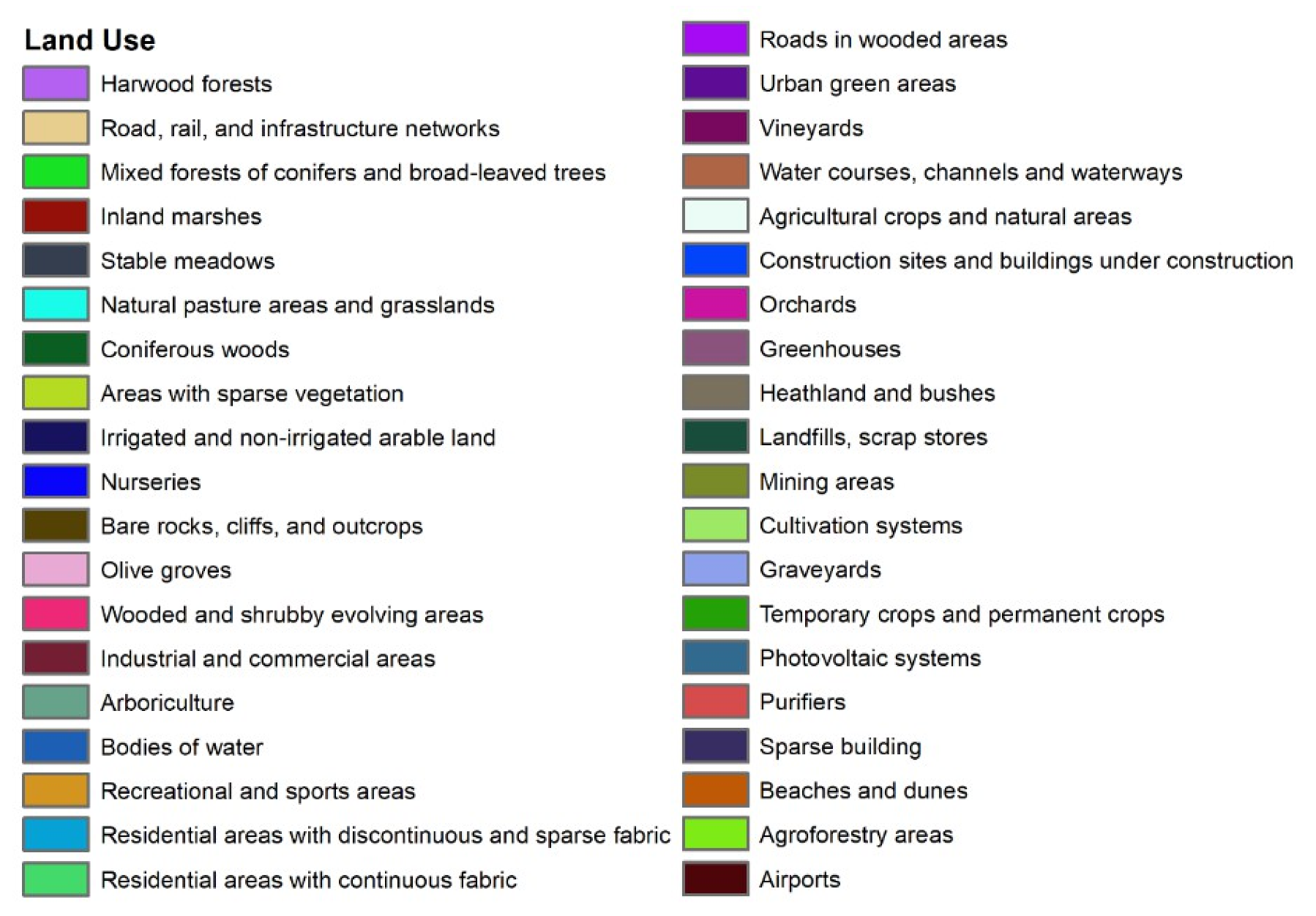
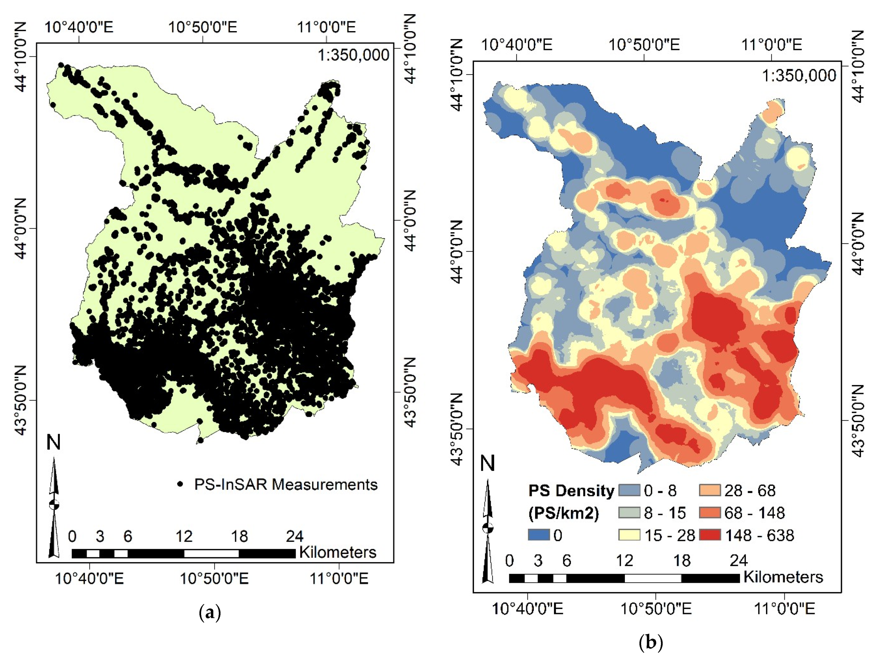
3.1. Study Area
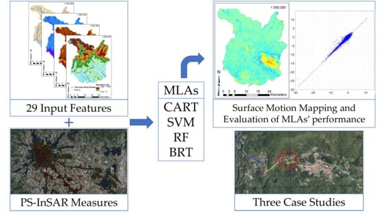
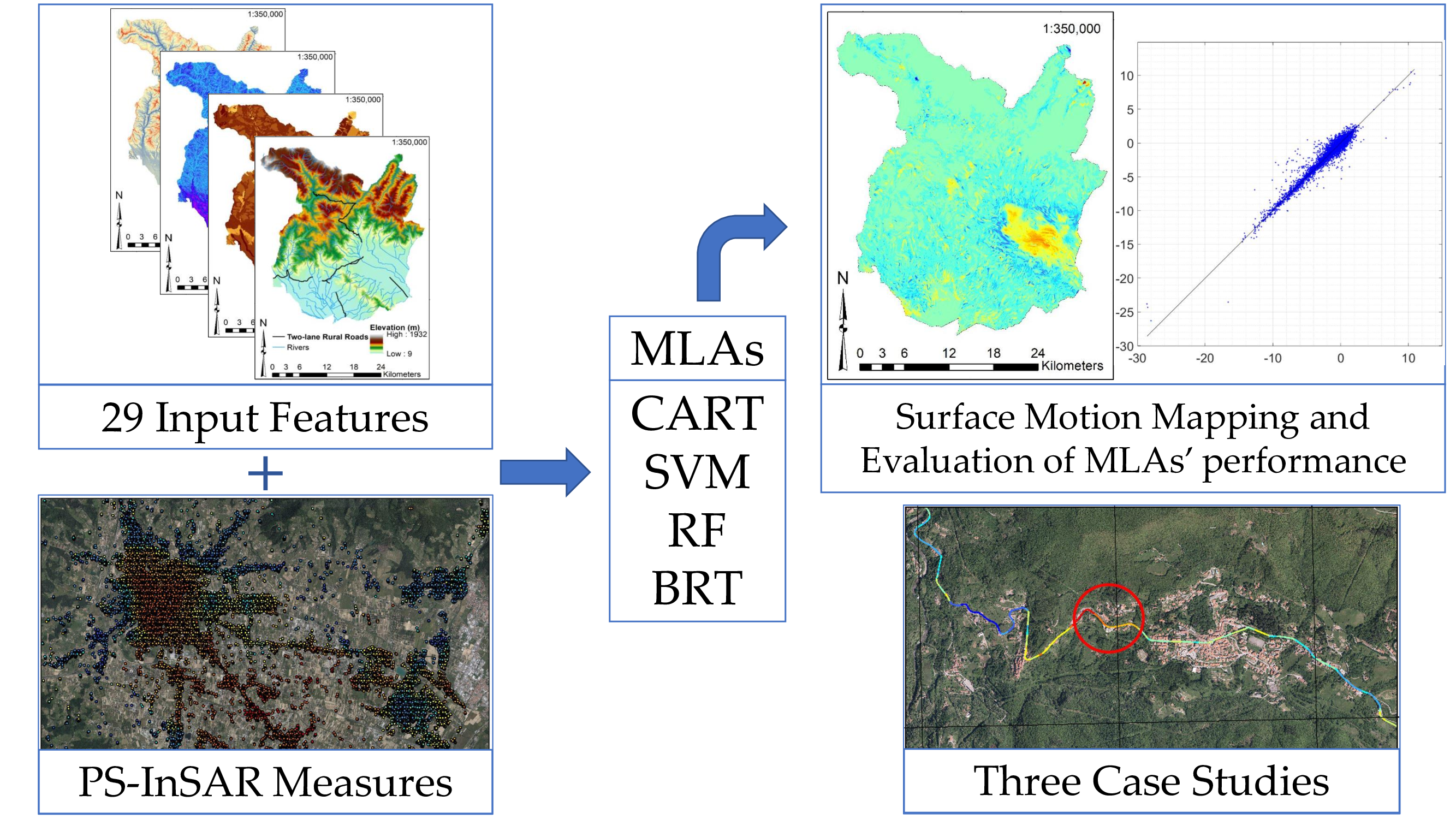
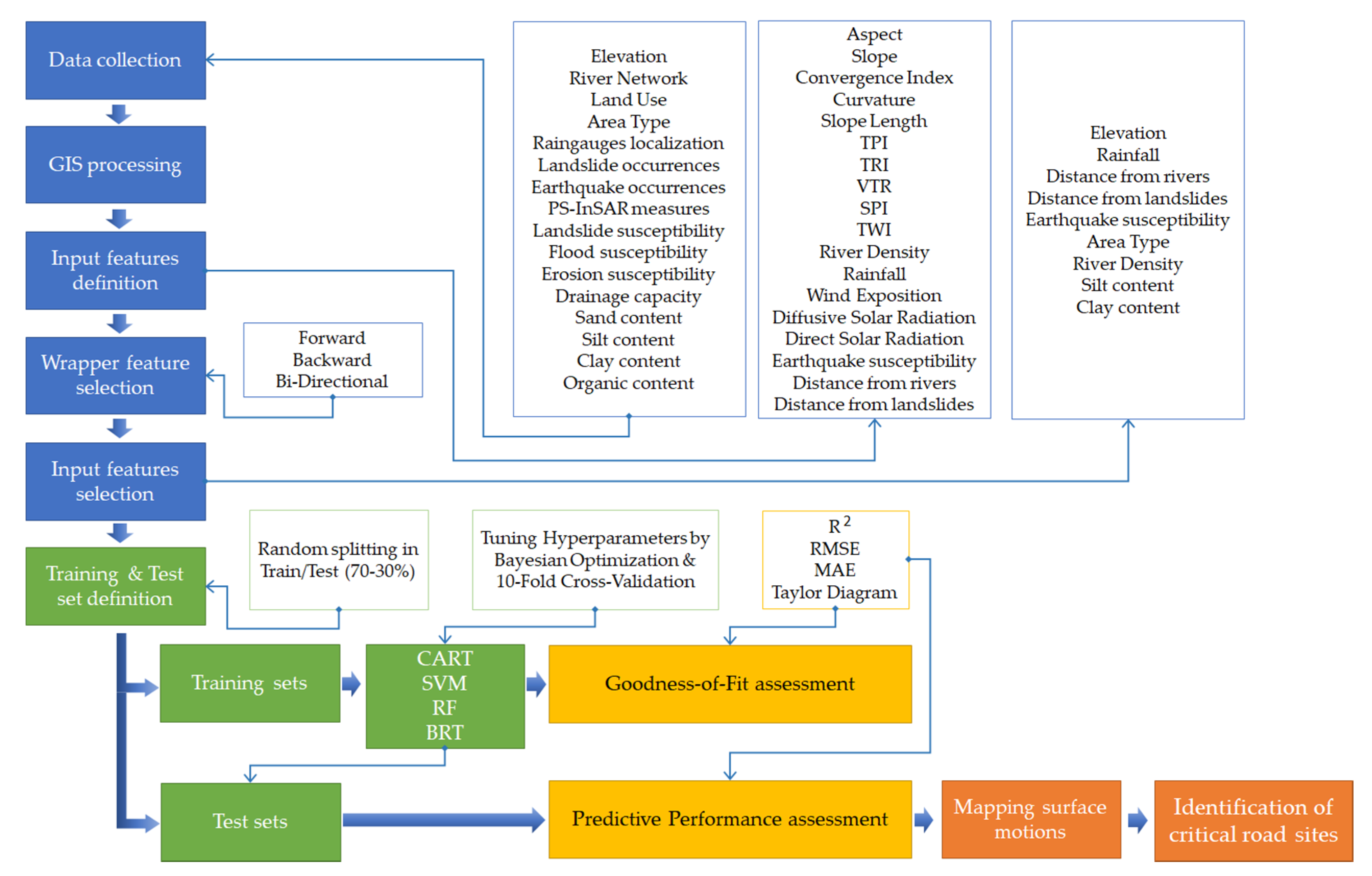
3.2. Workflow
3.3. Database Preparation
3.3.1. Data Collection
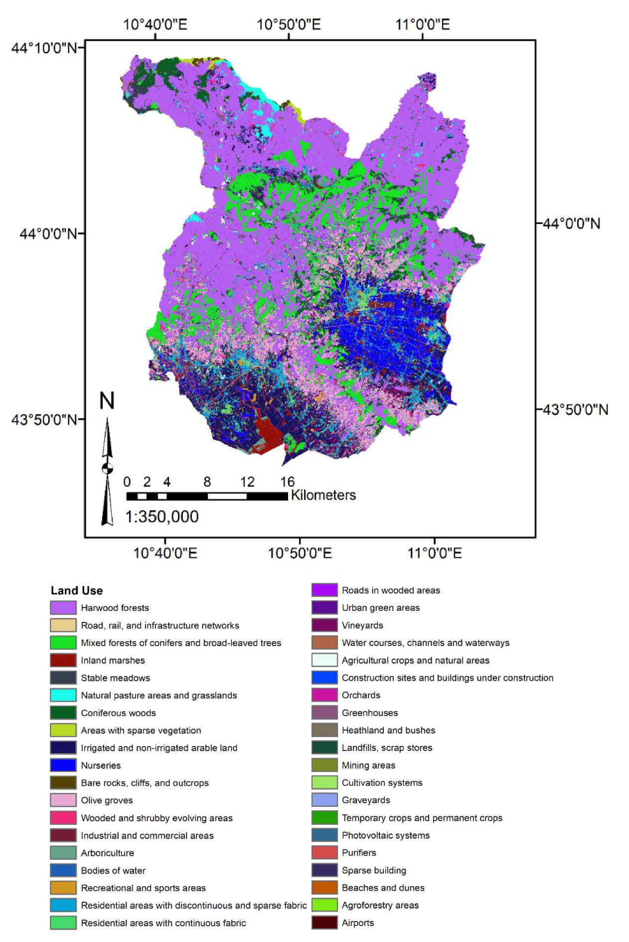
3.3.2. Definition of the Input Features and Data Aggregation
- Aspect and Slope (exploiting the Elevation) by their homonymous commands;
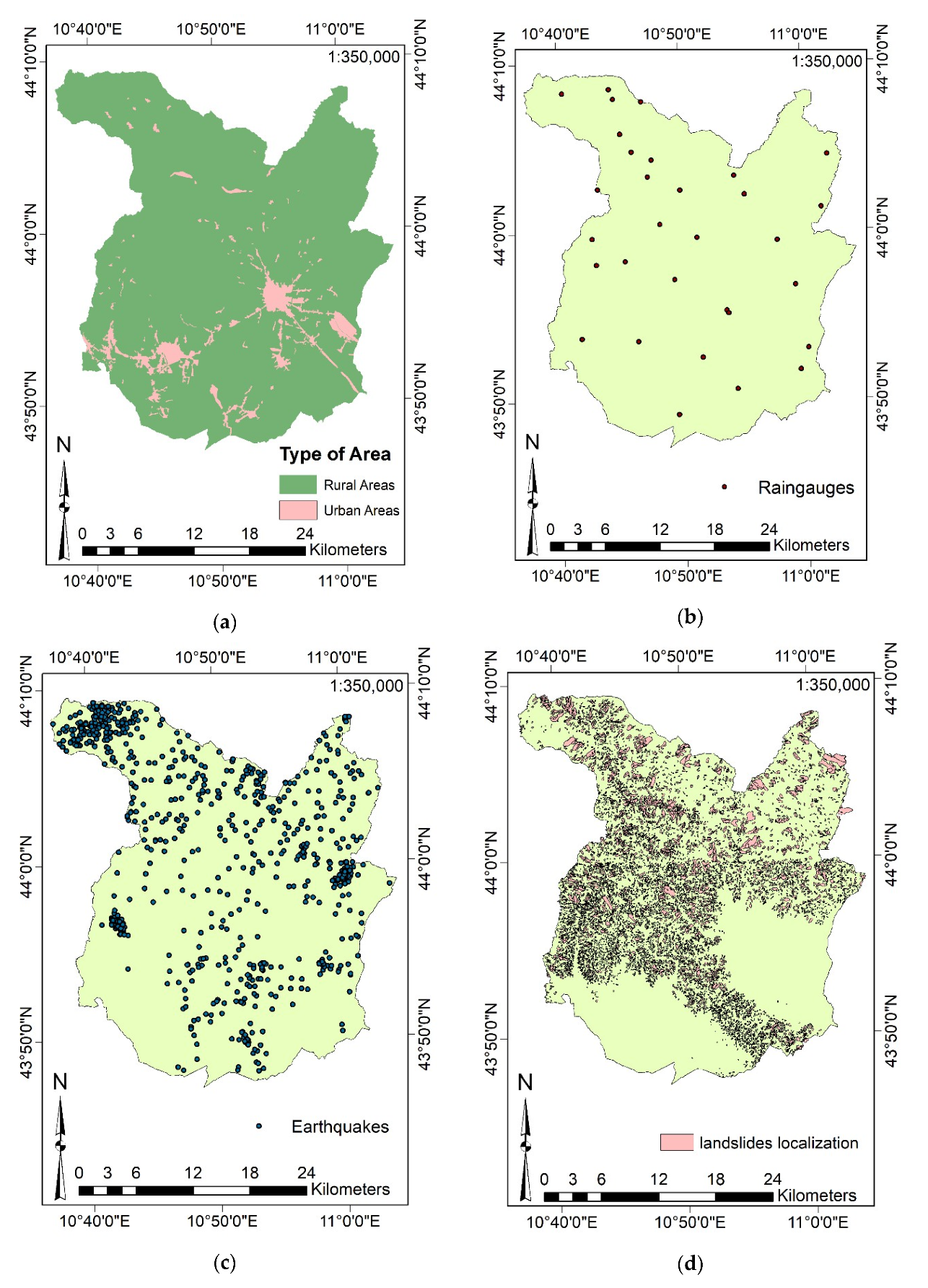
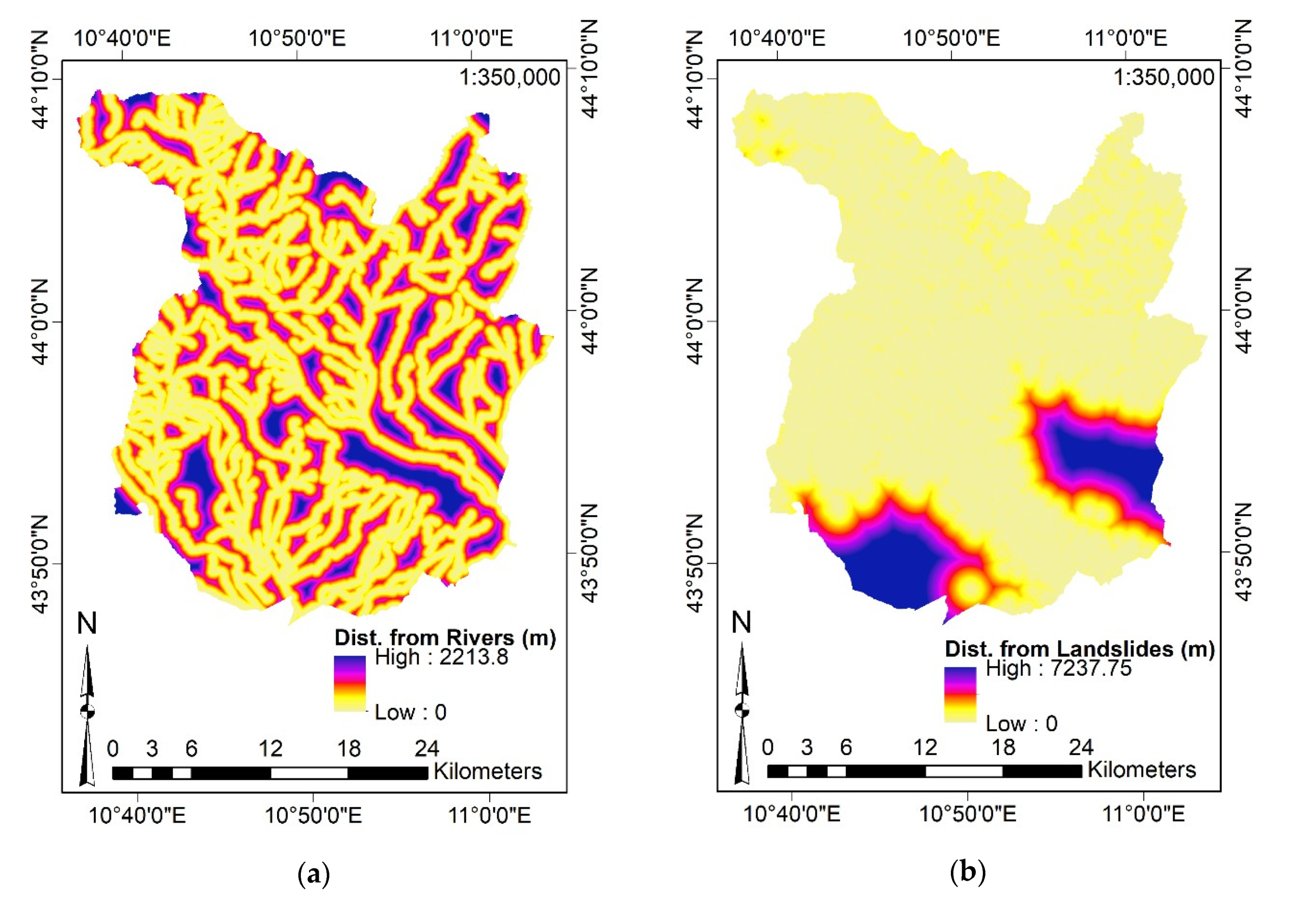
- Distance from Rivers and Distance from Landslides by the Euclidean Distance command (considering the landslides localization and the river network);
- River Density through the Kernel Density command (using the river network as input).
- Furthermore, SAGA-GIS software has been exploited for deriving:
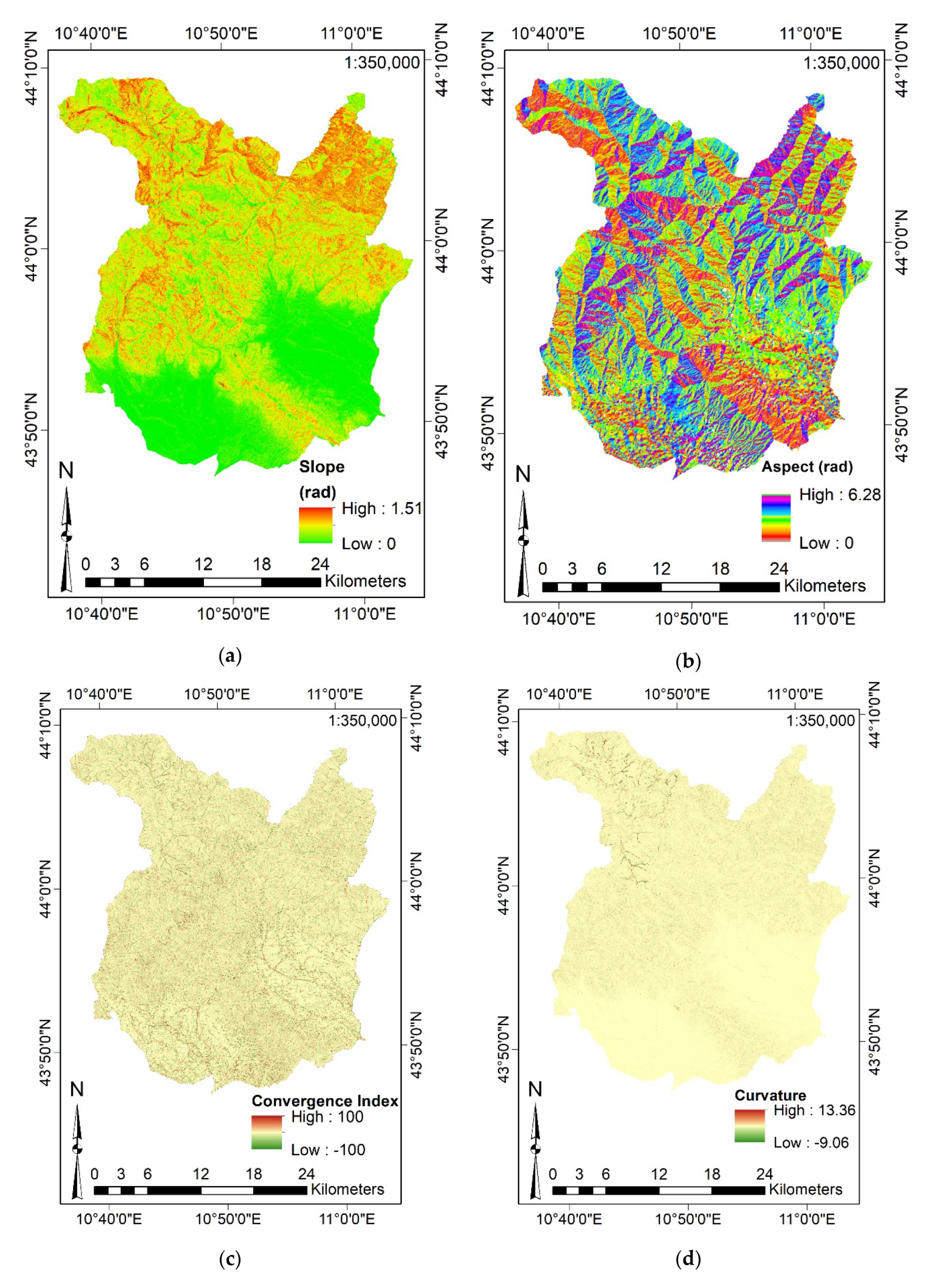
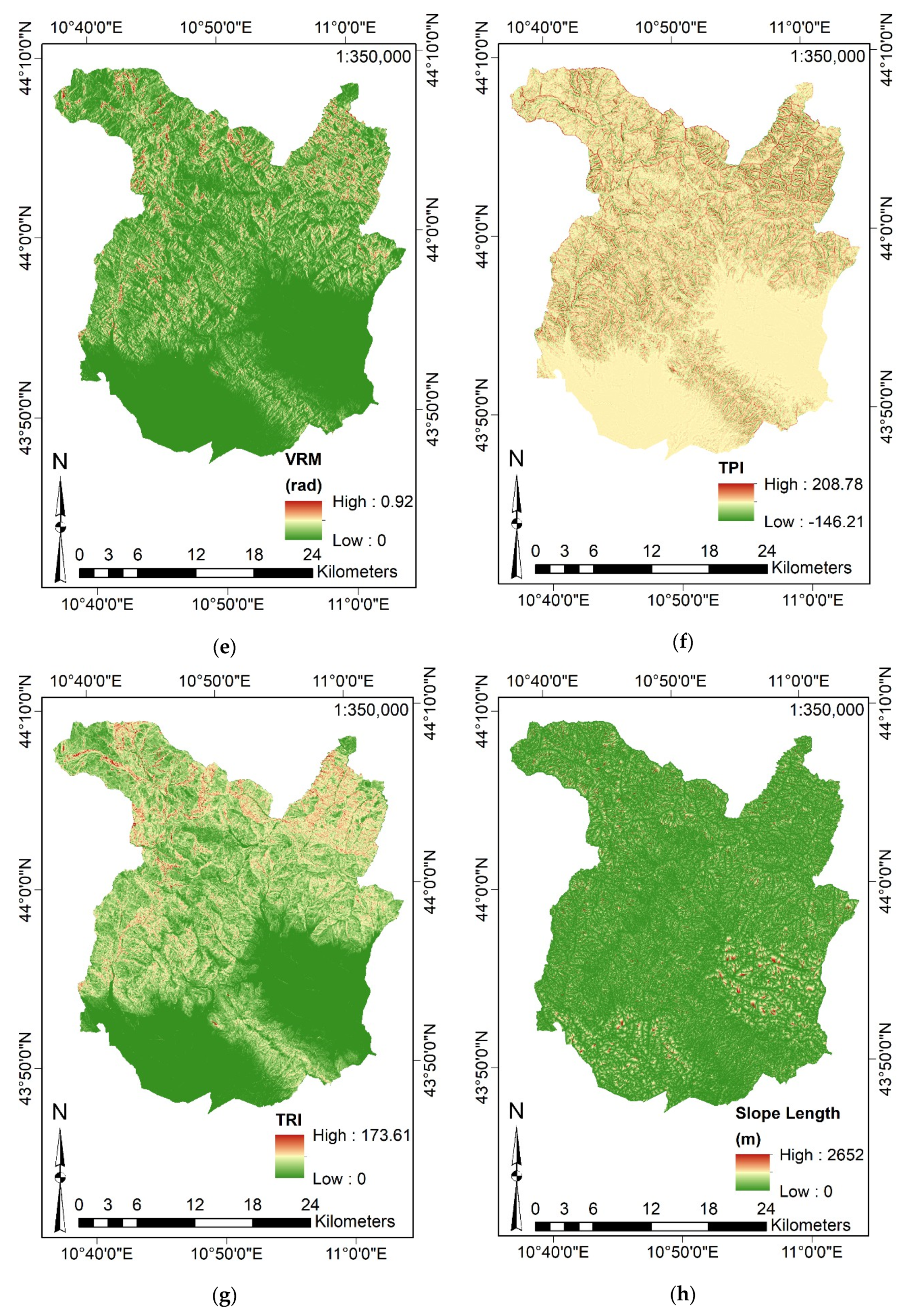
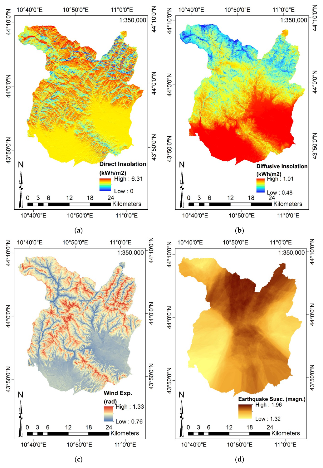
- CI, Curvature, VRM, TPI, TRI, SL, WE, Direct and Diffusive Solar Radiation by their homonymous commands (considering the Elevation);
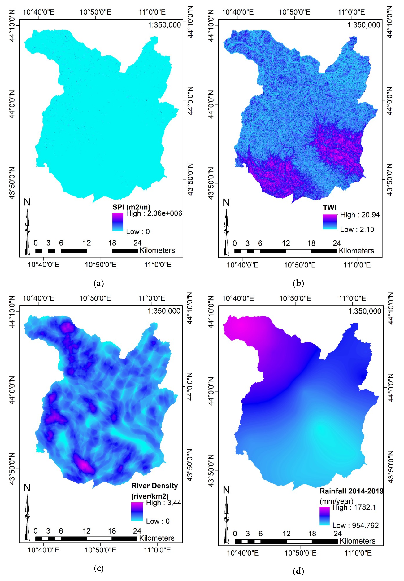
- SPI, TWI, by their homonymous commands (considering the Slope and the catchment area derived from the Elevation).
- CI:where describes the angle between the aspect of the i-th surrounding neighbor cell and the center cell (the cell under analysis) and is the number of neighbors (eight neighbor cells considering a 3-by-3 scheme);
- TPI:where is the elevation of the cell under analysis, is the elevation of the surrounding cells within a specified radius (100 m), and is the number of cells surrounding ,
- TRI:where is the elevation of each neighbor cell (eight neighbor cells considering a 3-by-3 scheme) to the elevation of the center cell (the cell under analysis);
- SL, SPI, and TWI:where is the specific area of the catchment (expressed as m2/m of catchment) and is the slope gradient (expressed in degrees). Equation (4) shows that SL is computed by knowing information on catchment area and slope; SAGA-GIS computes them internally by exploiting the Elevation.
- Slope represents the rate of change of the surface in horizontal and vertical directions from the cell under analysis;
- Aspect defines the slope direction. The values of Aspect of a cell indicates the compass direction (expressed in [rad] in the present paper) that the slope faces at that cell;
- Curvature is equal to the second derivative value of the input surface (the Elevation). For each cell, a fourth-order polynomial function is fit to a surface composed of a 3-by-3 window;
- VRM computes terrain ruggedness by measuring the dispersion of vectors orthogonal to each cell of the terrain input surface (Elevation). The cell under analysis and the eight surrounding neighbors are decomposed into three orthogonal components exploiting trigonometric relations, slope, and aspect. The VRM of the center cell (the cell under analysis) is equal to the magnitude of the resultant vector. Finally, the magnitude of the resultant vector is divided by the number of neighbor cells and subtracted from 1 (standardized and dimensionless form). Therefore, VRM ranges from 0 (flat) to 1 (most rugged) [120];
- WE is represented by the absolute angle distance between the aspect and the azimuth of wind flux considering the North direction as the reference. It considers surface orientation only, neglecting the influence of surrounding terrains as well as the slope. Accordingly, WE moves from 0° (windward) to 180° (leeward). In the present paper, it is expressed in its dimensionless form (i.e., values lesser than 1 define wind shadowed areas whereas values greater than 1 identify areas exposed to wind). Considering that the predominant wind directions were not known in advance, the averaged WE has been computed by imposing several hypothetic directions (i.e., for each 15°) [119];
- Direct Solar Radiation received from sun disk () and Diffuse Solar Radiation received by the sky’s hemisphere (), on an unobstructed horizontal surface, in clear-sky conditions, at an altitude , can be computed by Equations (7) and (8) exploiting the Elevation data [119]:where is the solar constant (1.367 kW/m2), is the air density integrated over distance from top of the atmosphere to the elevation , and is a coefficient for accounting the loss of absorbed exo-atmospheric solar energy when passing the atmosphere (in the present study, ).
3.3.3. Output Target Response
3.3.4. Definition of the Training and Test Sets
3.4. Feature Selection Approach
3.5. Machine Learning Algorithms
- CPU: Intel Core i9-9900 (8 core, 16 threads, 3.10 GHz, max 5 GHz);
- GPU: NVidia GeForce RTX 2080TI-11GB;
- SSD: Samsung 970 PRO 512 Mb;
- RAM memory: Corsair Vengeance LPX 32GB DDR4 3000 MHz (2 × 16 GB).
3.5.1. Regression Tree
3.5.2. Support Vector Machine
3.5.3. Random Forest
- RF algorithm exploits the bootstrap aggregation (also called Bagging) process, i.e., it defines several subsets of training samples with replacement, and then uses each of them for training each RT. For each subset, RF exploits two-thirds (in-bag samples) for training the RTs, and the remaining one-third (out-of-bag samples) for a CV process. This CV process is followed by the RF to minimize the error estimation (out-of-bag error) and define a robust algorithm;
- RF exploits the feature randomness approach, which is to choose a fixed number of input features randomly chosen to be used for defining the decision rules of each RT. Accordingly, each RT is trained by a different subset of input features. They have a high variance in their prediction and a low bias.
- The amount of RT structures constituting the forest: RF is not prone to overfit the data, then the number of decision trees can be enormous in order to enhance its performance. However, the higher the number of RT to train, the higher is the computational cost required for growing the RF. Moreover, the accuracy of RF does not significantly improve once a certain number of RT has been reached;
- The fixed number of input factors randomly sampled as candidates at each split.
3.5.4. Boosted Regression Tree
3.6. Hyperparameter Tuning by Bayesian Optimization Algorithm
- A set of evaluations of the function (training sample) is identified by imposing a Gaussian Process distribution and five random values of;
- The acquisition function is computed; the BOA identifies the next sample point that could improve the acquisition function and adds it to the training sample;
- The BOA updates the posterior distribution and computes the acquisition function again;
- At each new iteration, steps 1–3 are repeated, updating sequentially the with one new sample point per iteration; at each iteration, a new sample point is found and added to the training sample (the evidence data).
3.7. K-Fold Cross-Validation Procedure
3.8. Predictor Importance
- is the number of trees composing the forest;
- are the nodes belonging to the tree ;
- are the weighted impurity decreases;
- is the importance of the input feature
- is the proportion of samples reaching the node t;
- is the independent variable used in split .
3.9. Goodness-of-Fit and Predictive Performance Evaluation
- is the i-th predicted value of the target output ;
- is the i-th observed value of the target output ;
- is the averaged observed value of the target output .
4. Results and Discussion
4.1. Feature Selection
4.2. Machine Learning Hyperparameters
- CV process: 10-Fold;
- Optimization of the Hyperparameters: Bayesian Process, 30 iterations;
- Time for training the CART: 90 s;
- Fixed number of random variables to choose for splitting nodes: 9;
- Maximum number of splits: 8330;
- Minimum leaf nodes size: 2;
- Minimum parent size: 10;
- Split criterion: MSE;
- Number of nodes: 12,995;
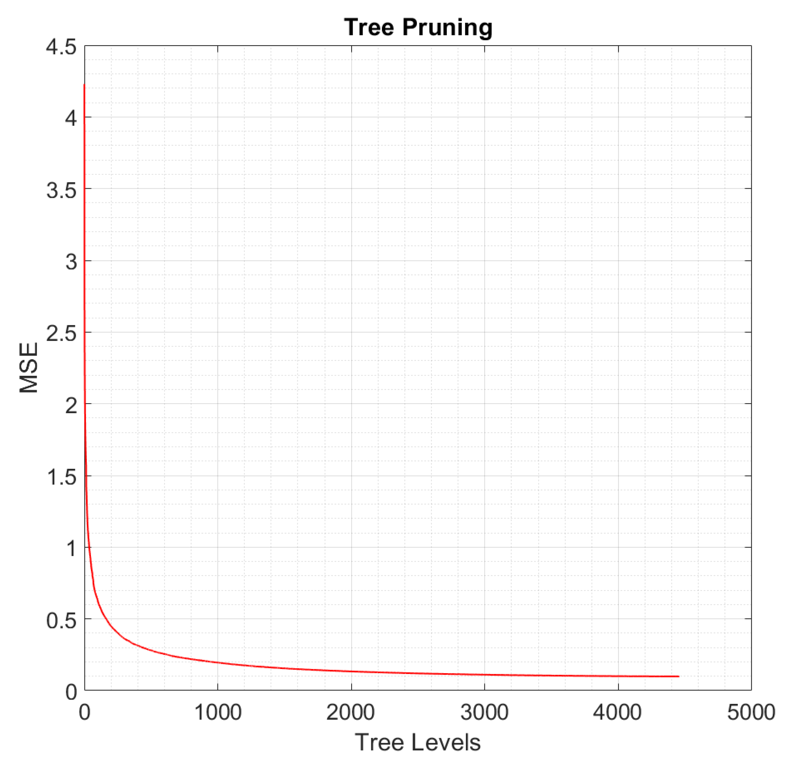
- Number of tree levels: 4457;
- Number of pruned levels: 2000 (according to Figure 6, if the RT is pruned by 2000 levels, the MSE does not increase significantly and the resulting RT is less complex and less prone to overfit data);
- Number of nodes after tree pruning: 6705 (2257 resulting tree levels).
- CV process: 10-Fold;
- Optimization of the Hyperparameters: Bayesian Process, 30 iterations;
- Time for training the SVM: 60,200 s;
- Standardize the input factors: yes;
- Type of kernel function: Gaussian kernel;
- C (Box constraint): 38.361;
- Gamma: 0.4017;
- Epsilon: 0.0012.
- CV process: 10-Fold;
- Optimization of the Hyperparameters: Bayesian Process, 30 iterations;
- Time for training the RF: 997 s;
- Fixed number of random variables to choose for splitting nodes: 9;
- Number of trees: 483;
- CV process: 10-Fold;
- Optimization of the Hyperparameters: Bayesian Process, 30 iterations;
- Time for training the BRT: 4285 s;
- Fixed number of random variables to choose for splitting nodes: 9;
- Number of learning cycles: 248;
- Learning rate: 0.1042;
- Maximum number of splits: 1470;
- Minimum size of the leaf nodes: 6;
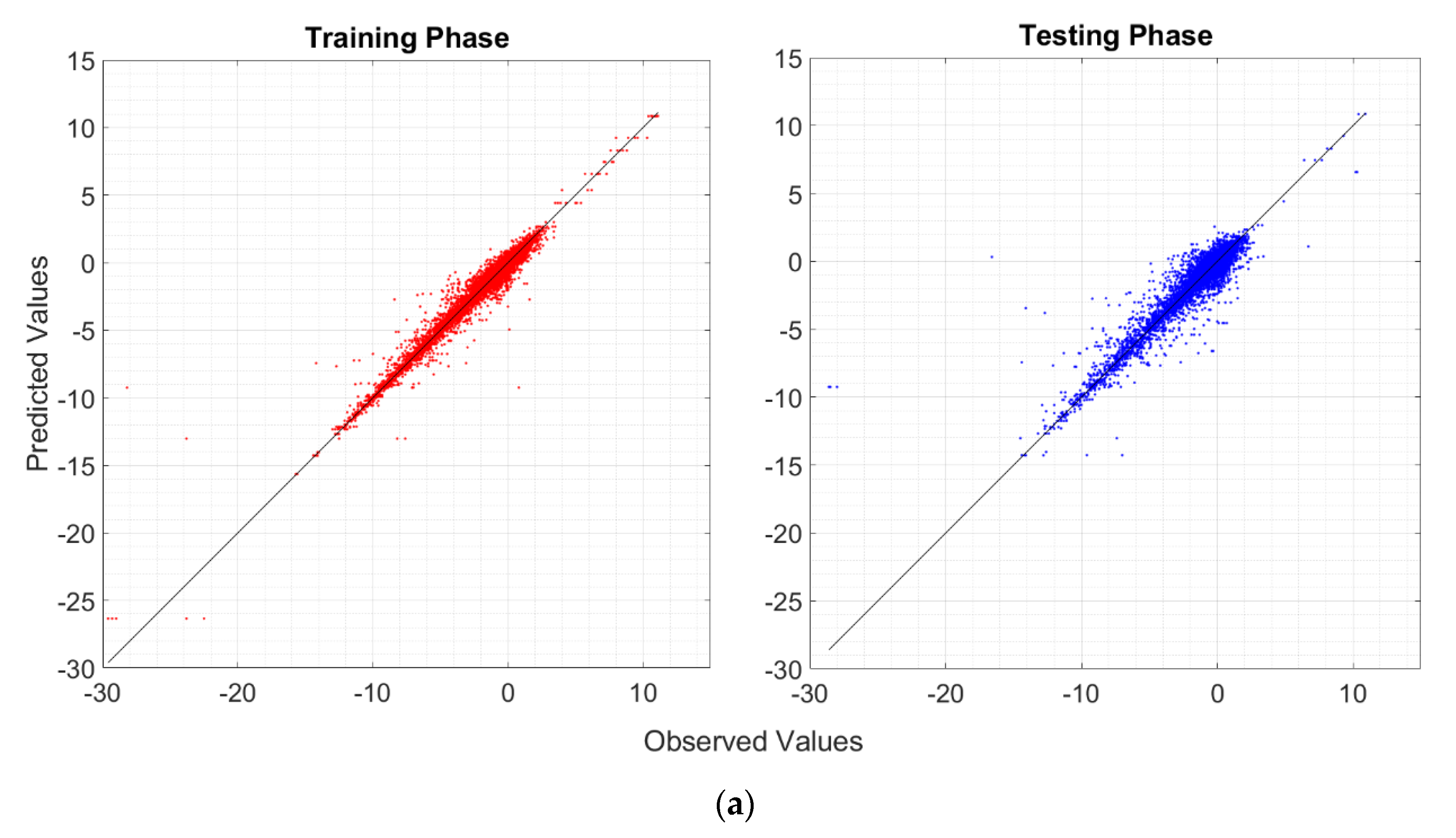
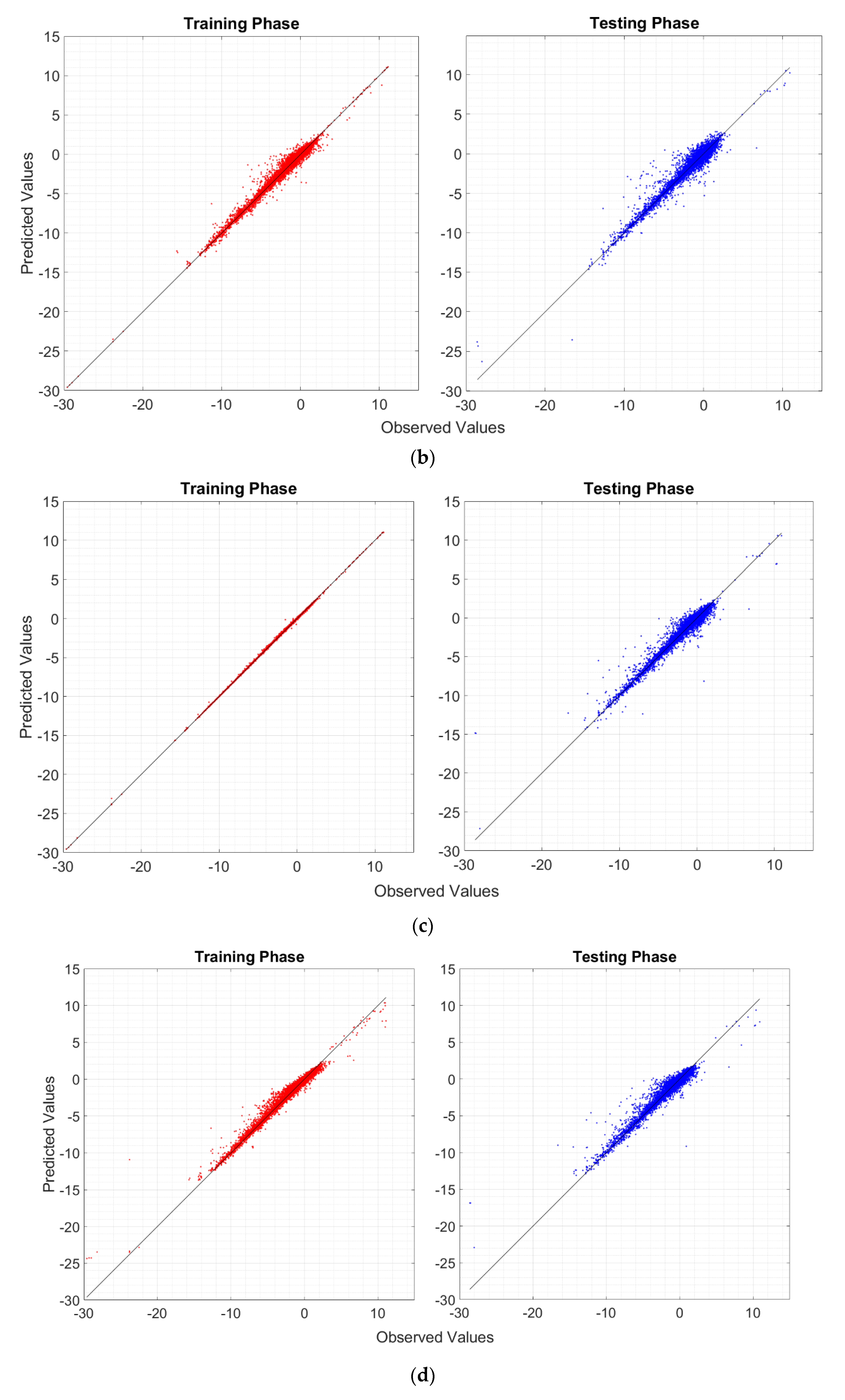
4.3. Goodness-of-Fit and Predictive Performance Assessment
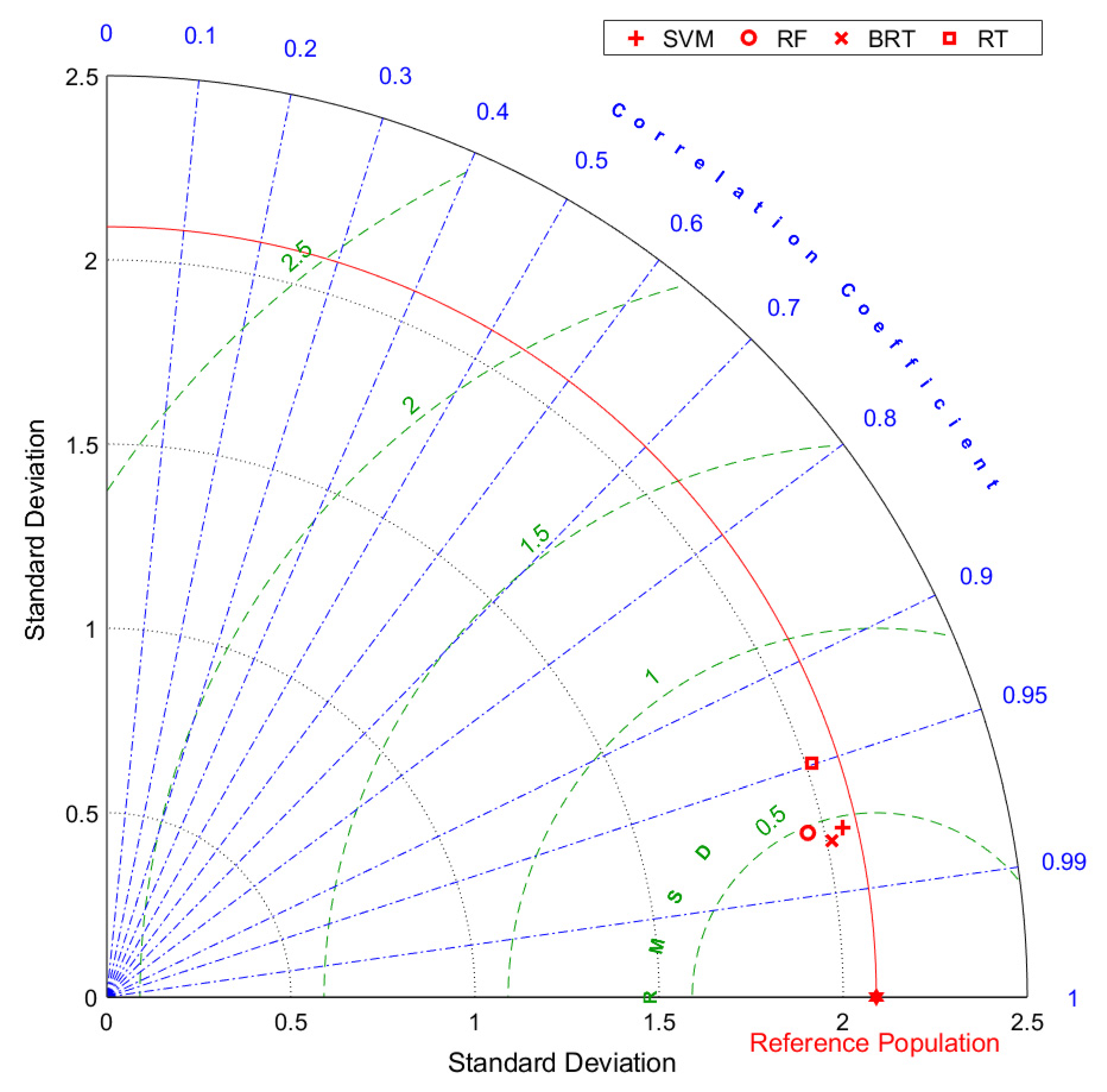
- RF is not fully able to explain the variability of the target output, although the R2, RMSE, and MAE are satisfactory both during the training and testing phases;
- RT and BRT may overfit the data during the training phase. Nonetheless, BRT shows adequate performance in the testing phase, comparable to those of the other algorithms (SVM and RF);
- The R2, RMSE, and MAE reveals that RT is worse than the other MLAs for making predictions, and it should not be used in favor of more complex algorithms;
- It appears that SVM does not overfit the data during the training phase. Moreover, during both training and test phases, SVM is one of the most reliable MLAs (preceded only by the BRT), and it has the most similar standard deviation compared to that of the reference population;
- Considering the potential overfitting issues of the BRT, the SVM should be the most suitable and reliable algorithm for making predictions.
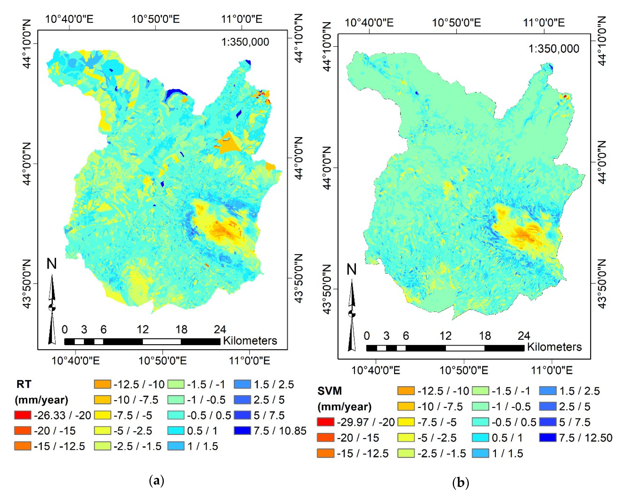
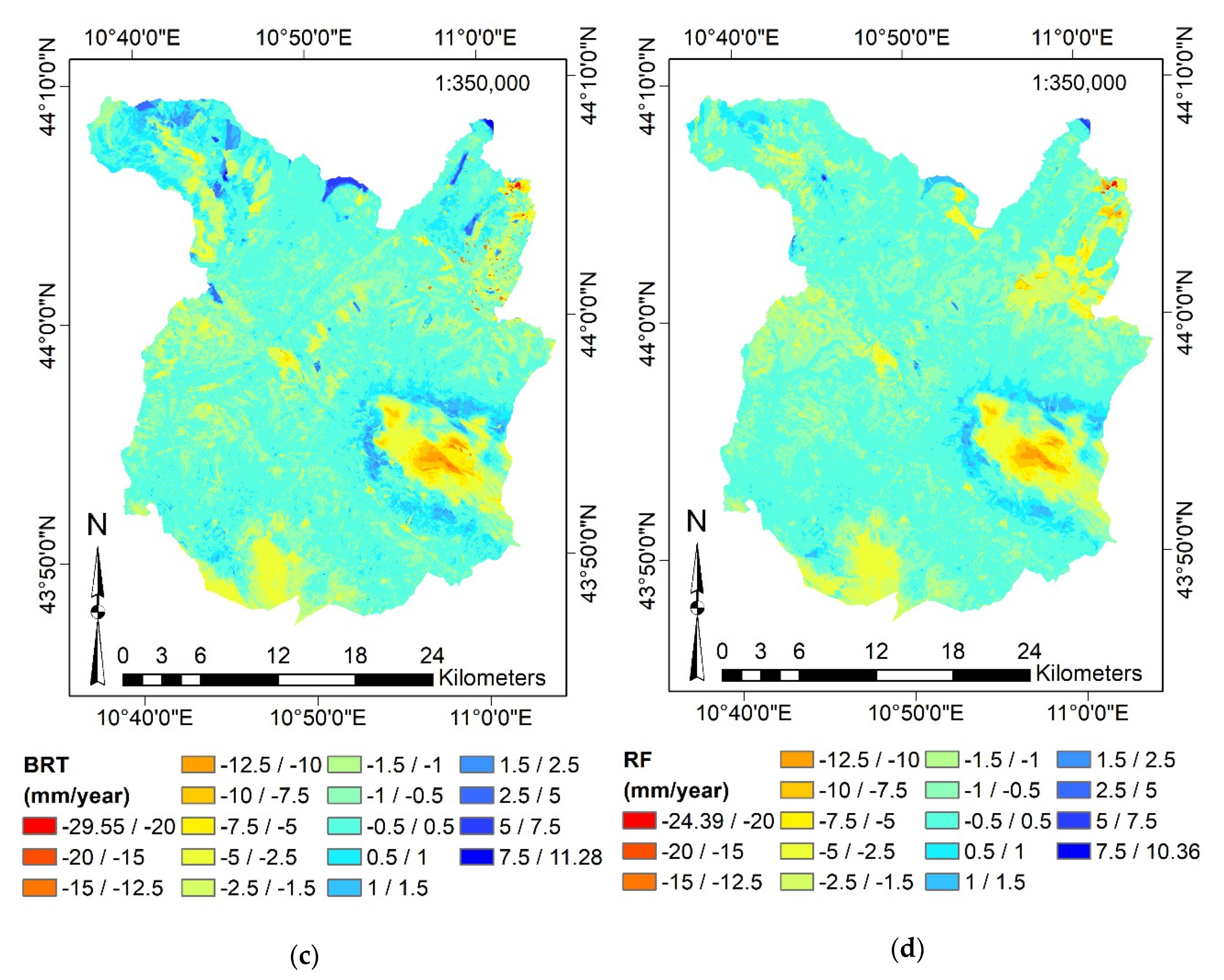
4.4. Surface Motion Estimations
4.5. Predictor Importance
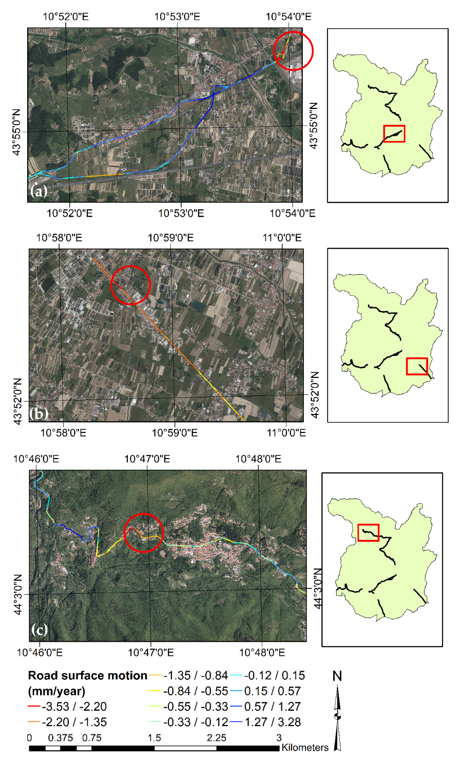
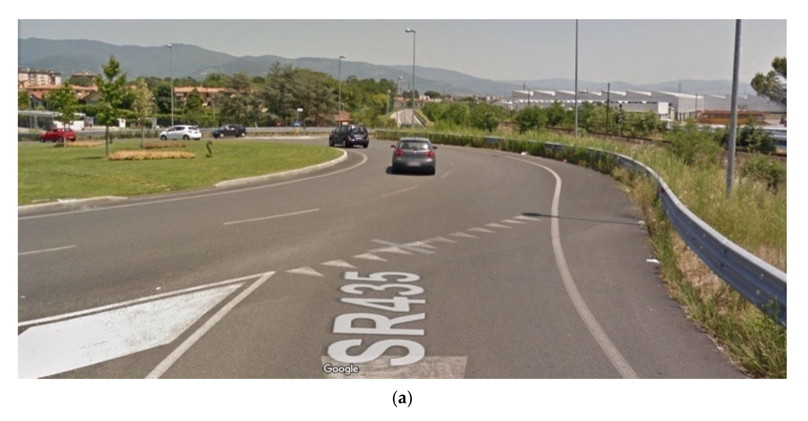
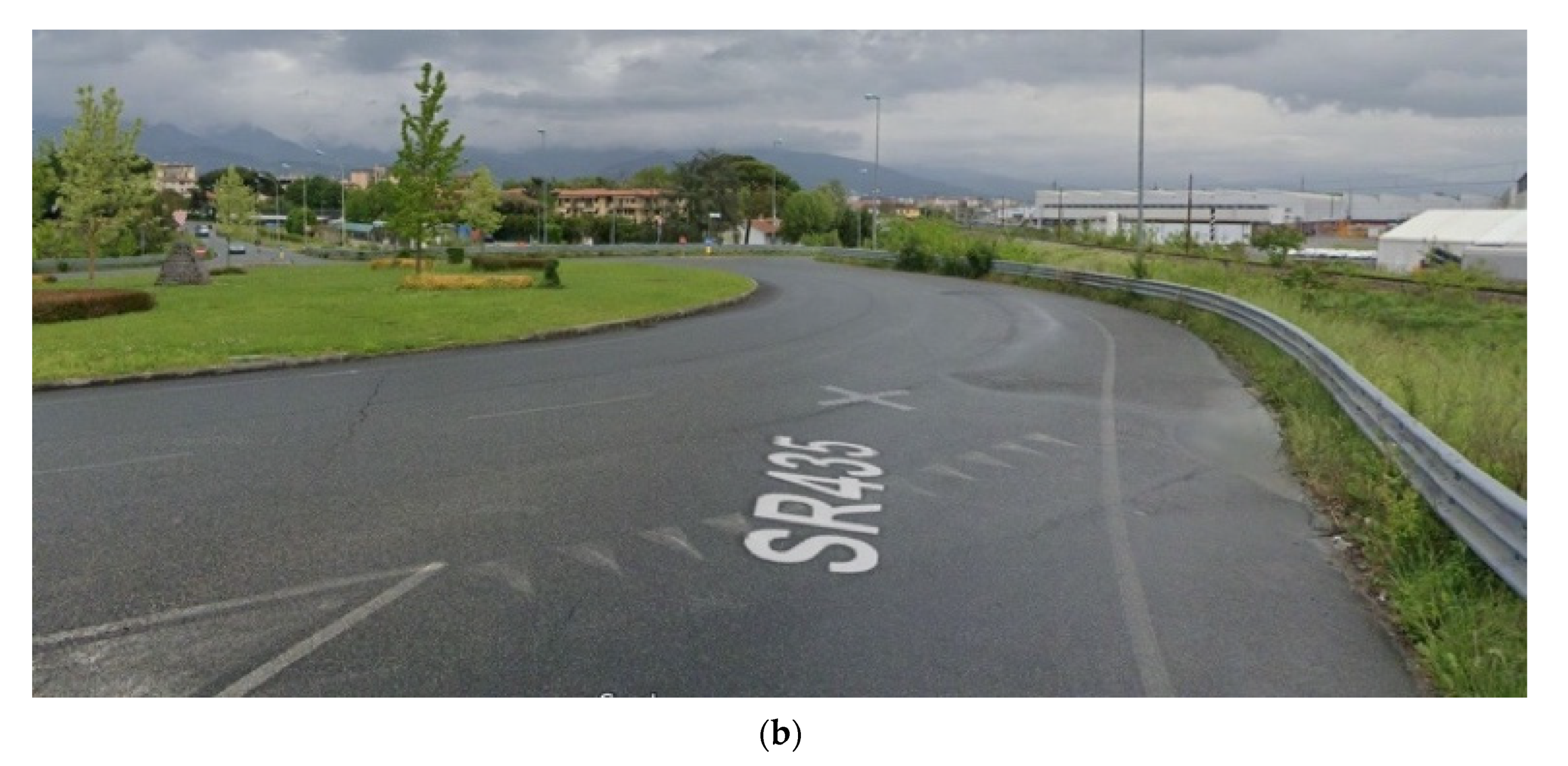
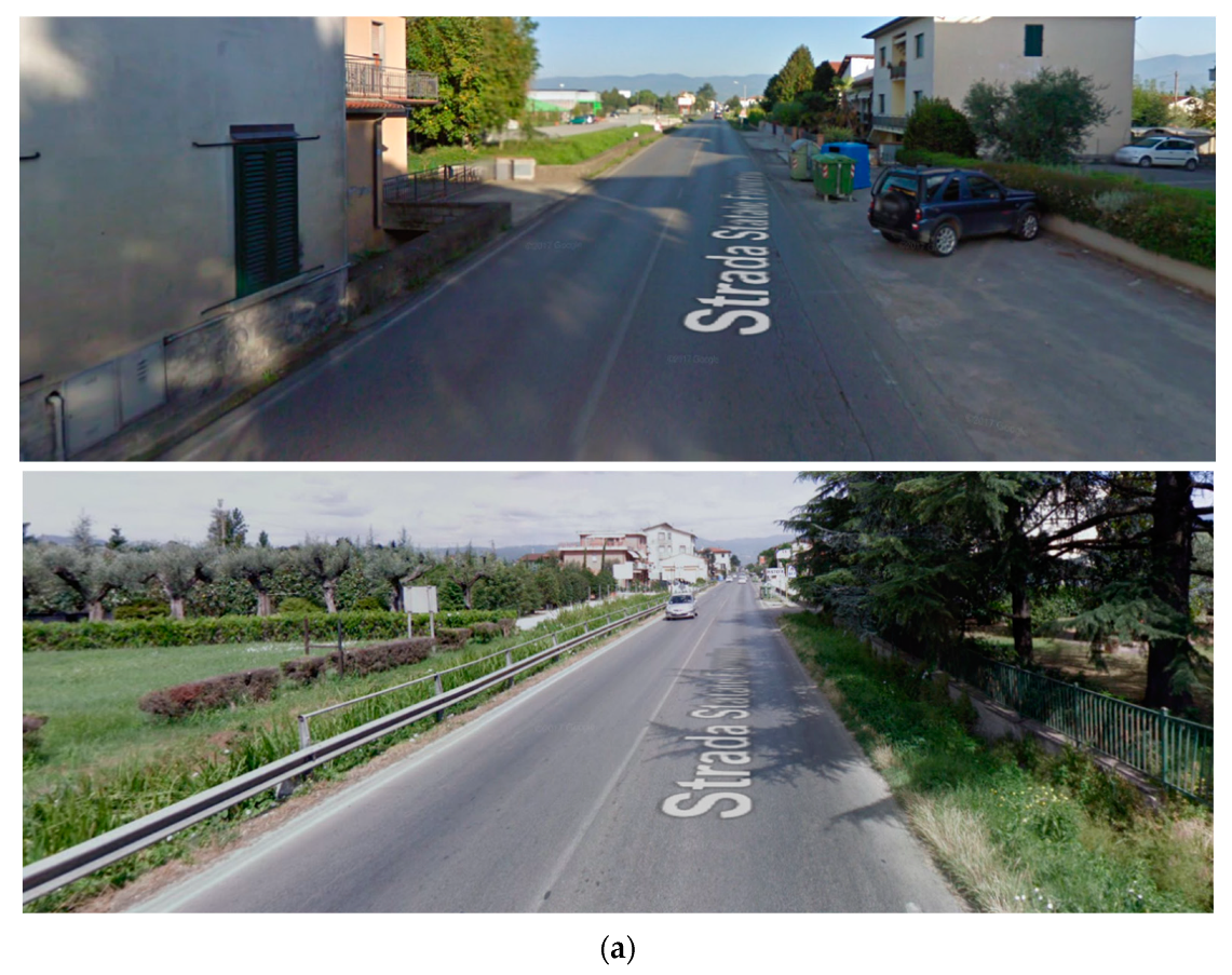
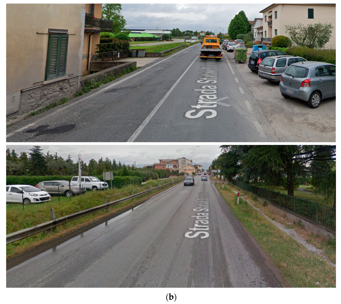
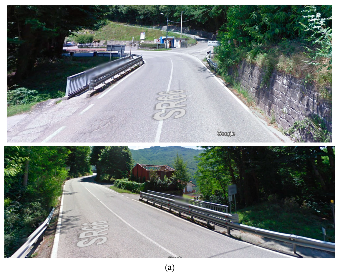
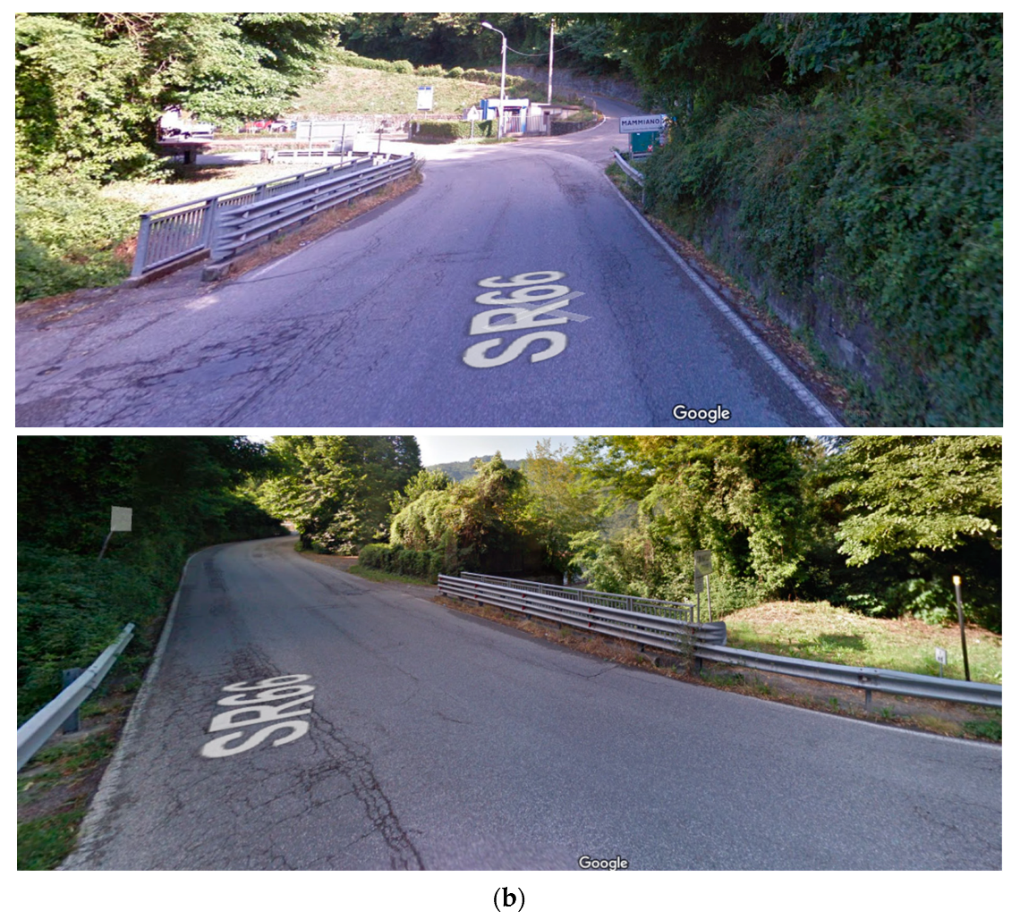
4.6. Validation on Stretches of Two-lane Rural Roads
4.7. Use of the Procedure by Road Authorities
- It allows quantifying the surface motion of road pavements in every point of the infrastructures, even in those areas where there is no presence of PS detected by InSAR techniques; road authorities could use the calibrated MLAs in other areas than where they were trained;
- The most influential and relevant factors on the deterioration of pavements connected to environmental and social parameters can be quantified. Consequently, road authorities can arrange appropriate and specific maintenance interventions that also consider exogenous factors;
- Monitoring and inspection activities of complex and extensive networks can be carried out with a sufficient degree of accuracy, a high level of detail, and low cost (once the procedure has been calibrated). Nonetheless, the methodology cannot replace modern Non-Destructive High-Performance Techniques, such as Falling Weight Deflectometer, Ground Penetrating Radar, or Profilometric measurements. However, thanks to the findings suggested by the procedure, road authorities may have a tool for identifying a reduced set of road sites to be inspected. Once specific admissibility thresholds of displacement (both negative and positive) have been set, those road sites that require more attention will be automatically extracted;
- By this procedure, road authorities may have more objective criteria for the planning of new infrastructures. Indeed, thanks to the surface motion maps, it is possible to identify the areas in which building a new infrastructure may be inappropriate. If admissibility thresholds are set for this activity, different categories of areas could be discovered, such as good, acceptable, not recommended, or prohibited areas for the development of a new infrastructural corridor;
4.8. Future Works
- Extend the study area to different Provinces, up to the mapping of the entire Tuscany Region (23,000 km2), relying on over 830,000 PS;
- It would be advisable to integrate information relating to the ascending and descending orbit to estimate the surface motion ratio in the vertical direction and not in the Line-Of-Sight direction of the sensor;
- Consider the entire road network present in the study area (including the urban sections of the two-lane rural roads and other roads not managed by the TRRA);
- Consider also the railway network, extending the field of use to all the so-called linear infrastructures;
- Test different feature selection approaches, such as the PCA, and compare the results obtained with the wrapper approaches implemented in this study;
- Calibration of more complex MLAs, such as Neural Networks (both Multilayer Perceptron and Convolutional Neural Networks), and comparison with the already implemented MLAs. Furthermore, algorithms related to the stacking technique could be developed (i.e., parallel and independent training of various learners and the aggregation of their predictions by another MLA, whose inputs are learners’ predictions).
5. Conclusions
Author Contributions
Funding
Acknowledgments
Conflicts of Interest
Appendix A


References
- Maboudi, M.; Amini, J.; Hahn, M.; Saati, M. Object-based road extraction from satellite images using ant colony optimization. Int. J. Remote Sens. 2017, 38, 179–198. [Google Scholar] [CrossRef]
- Fiorentini, N.; Maboudi, M.; Losa, M.; Gerke, M. Assessing Resilience of Infrastructures Towards Exogenous Events by Using PS-InSAR-Based Surface Motion Estimates and Machine Learning Regression Techniques. ISPRS Ann. Photogramm. Remote Sens. Spat. Inf. Sci. 2020, 4, 19–26. [Google Scholar] [CrossRef]
- Ouchi, K. Recent Trend and Advance of Synthetic Aperture Radar with Selected Topics. Remote Sens. 2013, 5, 716–807. [Google Scholar] [CrossRef] [Green Version]
- Graham, L.C. Synthetic Interferometer Radar For Topographic Mapping. Proc. IEEE 1974. [Google Scholar] [CrossRef]
- Costantini, M.; Ferretti, A.; Minati, F.; Falco, S.; Trillo, F.; Colombo, D.; Novali, F.; Malvarosa, F.; Mammone, C.; Vecchioli, F.; et al. Analysis of surface deformations over the whole Italian territory by interferometric processing of ERS, Envisat and COSMO-SkyMed radar data. Remote Sens. Environ. 2017, 202, 250–275. [Google Scholar] [CrossRef]
- Ferretti, A.; Prati, C.; Rocca, F. Permanent Scatterers in SAR Interferometry. IEEE Trans. Geosci. Remote Sens. 2001, 39, 8–20. [Google Scholar] [CrossRef]
- Ferretti, A.; Prati, C.; Rocca, F. Nonlinear Subsidence Rate Estimation Using Permanent Scatterers in Differential SAR Interferometry. IEEE Trans. Geosci. Remote Sens. 2000, 38, 2202–2212. [Google Scholar] [CrossRef] [Green Version]
- Ferretti, A.; Monti-Guarnieri, A.; Prati, C.; Rocca, F. InSAR Principles: Guidelines for SAR Interferometry Processing and Interpretation; TM-19; ESA Publications: Auckland, New Zealand, 2007. [Google Scholar]
- Gheorghe, M.; Armaş, I. Comparison of Multi-Temporal Differential Interferometry Techniques Applied to the Measurement of Bucharest City Subsidence. Procedia Environ. Sci. 2016, 32, 221–229. [Google Scholar] [CrossRef] [Green Version]
- Milczarek, W.; Blachowski, J.; Grzempowski, P. Application of Psinsar For Assessment of Surface Deformations in Post-Mining Area-Case Study of the Former Walbrzych Hard Coal Basin (Sw Poland). Acta Geodyn. Geomater. 2017, 14, 41–52. [Google Scholar] [CrossRef]
- Samsonov, S.; d’Oreye, N.; Smets, B. Ground deformation associated with post-mining activity at the French-German border revealed by novel InSAR time series method. Int. J. Appl. Earth Obs. Geoinf. 2013. [Google Scholar] [CrossRef]
- Perissin, D.; Wang, Z.; Lin, H. Shanghai subway tunnels and highways monitoring through Cosmo-SkyMed Persistent Scatterers. ISPRS J. Photogramm. Remote Sens. 2012, 73, 58–67. [Google Scholar] [CrossRef]
- Wang, H.; Feng, G.; Xu, B.; Yu, Y.; Li, Z.; Du, Y.; Zhu, J. Deriving spatio-temporal development of ground subsidence due to subway construction and operation in Delta regions with PS-InSAR data: A case study in Guangzhou, China. Remote Sens. 2017, 9, 1004. [Google Scholar] [CrossRef] [Green Version]
- Xavier, D.; Declercq, P.-Y.; Bruno, F.; Jérôme, B.; Albert, T.; Julien, V. Uplift Revealed by Radar Interferometry Around Liege (Belgium): A Relation with Rising Mining Groundwater. Post Mining 2008, 6–8. [Google Scholar]
- Solari, L.; Del Soldato, M.; Bianchini, S.; Ciampalini, A.; Ezquerro, P.; Montalti, R.; Raspini, F.; Moretti, S. From ERS 1/2 to Sentinel-1: Subsidence Monitoring in Italy in the Last Two Decades. Front. Earth Sci. 2018, 6, 149. [Google Scholar] [CrossRef]
- Rosi, A.; Tofani, V.; Agostini, A.; Tanteri, L.; Tacconi Stefanelli, C.; Catani, F.; Casagli, N. Subsidence mapping at regional scale using persistent scatters interferometry (PSI): The case of Tuscany region (Italy). Int. J. Appl. Earth Obs. Geoinf. 2016, 52, 328–337. [Google Scholar] [CrossRef]
- Del Soldato, M.; Farolfi, G.; Rosi, A.; Raspini, F.; Casagli, N. Subsidence Evolution of the Firenze–Prato–Pistoia Plain (Central Italy) Combining PSI and GNSS Data. Remote Sens. 2018, 10, 1146. [Google Scholar] [CrossRef] [Green Version]
- Benattou, M.M.; Balz, T.; Minsheng, L. Measuring Surface Subsidence in Wuhan, China with Sentinel-1 Data Using Psinsar. In Proceedings of the 2018 ISPRS TC III Mid-term Symposium Developments, Technologies and Applications in Remote Sensing, Beijing, China, 7–10 May 2018. [Google Scholar] [CrossRef] [Green Version]
- Ng, A.H.-M.; Ge, L.; Li, X.; Abidin, H.Z.; Andreas, H.; Zhang, K. Mapping land subsidence in Jakarta, Indonesia using persistent scatterer interferometry (PSI) technique with ALOS PALSAR. Int. J. Appl. Earth Obs. Geoinf. 2012, 18, 232–242. [Google Scholar] [CrossRef]
- Comerci, V.; Vittori, E.; Cipolloni, C.; Di Manna, P.; Guerrieri, L.; Nisio, S.; Succhiarelli, C.; Ciuffreda, M.; Bertoletti, E. Geohazards Monitoring in Roma from InSAR and In Situ Data: Outcomes of the PanGeo Project. Pure Appl. Geophys. 2015. [Google Scholar] [CrossRef]
- Bianchini, S.; Pratesi, F.; Nolesini, T.; Casagli, N. Building Deformation Assessment by Means of Persistent Scatterer Interferometry Analysis on a Landslide-Affected Area: The Volterra (Italy) Case Study. Remote Sens. 2015, 7, 4678–4701. [Google Scholar] [CrossRef] [Green Version]
- Wasowski, J.; Bovenga, F. Investigating landslides and unstable slopes with satellite Multi Temporal Interferometry: Current issues and future perspectives. Eng. Geol. 2014, 174, 103–138. [Google Scholar] [CrossRef]
- Rosi, A.; Tofani, V.; Tanteri, L.; Tacconi Stefanelli, C.; Agostini, A.; Catani, F.; Casagli, N. The new landslide inventory of Tuscany (Italy) updated with PS-InSAR: Geomorphological features and landslide distribution. Landslides 2018. [Google Scholar] [CrossRef] [Green Version]
- Yin, Y.; Zheng, W.; Liu, Y.; Zhang, J.; Li, X. Integration of GPS with InSAR to monitoring of the Jiaju landslide in Sichuan, China. Landslides 2010. [Google Scholar] [CrossRef]
- Schlögel, R.; Doubre, C.; Malet, J.P.; Masson, F. Landslide deformation monitoring with ALOS/PALSAR imagery: A D-InSAR geomorphological interpretation method. Geomorphology 2015, 231, 314–330. [Google Scholar] [CrossRef]
- Béjar-Pizarro, M.; Notti, D.; Mateos, R.M.; Ezquerro, P.; Centolanza, G.; Herrera, G.; Bru, G.; Sanabria, M.; Solari, L.; Duro, J.; et al. Mapping vulnerable urban areas affected by slow-moving landslides using Sentinel-1InSAR data. Remote Sens. 2017, 9, 876. [Google Scholar] [CrossRef] [Green Version]
- Riedel, B.; Walther, A. InSAR processing for the recognition of landslides. Adv. Geosci. 2008. [Google Scholar] [CrossRef] [Green Version]
- Hoppe, E.; Bruckno, B.; Campbell, E.; Acton, S.; Vaccari, A.; Stuecheli, M.; Bohane, A.; Falorni, G.; Morgan, J. Transportation Infrastructure Monitoring Using Satellite Remote Sensing. In Materials and Infrastructures 1; John Wiley & Sons, Inc.: Hoboken, NJ, USA, 2016; pp. 185–198. [Google Scholar]
- Galve, J.P.; Castañeda, C.; Gutiérrez, F. Railway deformation detected by DInSAR over active sinkholes in the Ebro Valley evaporite karst, Spain. Hazards Earth Syst. Sci. 2015, 15, 2439–2448. [Google Scholar] [CrossRef] [Green Version]
- Galve, J.P.; Castañeda, C.; Gutiérrez, F.; Herrera, G. Assessing sinkhole activity in the Ebro Valley mantled evaporite karst using advanced DInSAR. Geomorphology 2015, 229, 30–44. [Google Scholar] [CrossRef] [Green Version]
- Ferentinou, M.; Witkowski, W.; Hejmanowski, R.; Grobler, H.; Malinowska, A. Detection of sinkhole occurrence, experiences from South Africa. Proc. Int. Assoc. Hydrol. Sci. 2020, 382, 77–82. [Google Scholar] [CrossRef] [Green Version]
- Villarroel, C.D.; Beliveau, G.T.; Forte, A.P.; Monserrat, O.; Morvillo, M. DInSAR for a regional inventory of active rock glaciers in the Dry Andes Mountains of Argentina and Chile with sentinel-1 data. Remote Sens. 2018, 10, 1588. [Google Scholar] [CrossRef] [Green Version]
- Nagler, T.; Mayer, C.; Rott, H. Feasibility of DINSAR for mapping complex motion fields of alpine ice- and rock-glaciers. In Proceedings of the Third International Symposium on Retrieval of Bio- and Geophysical Parameters from SAR Data for Land Applications, Sheffield, UK, 11–14 September 2001. [Google Scholar]
- Reinosch, E.; Buckel, J.; Dong, J.; Gerke, M.; Baade, J.; Riedel, B. InSAR time series analysis of seasonal surface displacement dynamics on the Tibetan Plateau. Cryosph. 2020, 14, 1633–1650. [Google Scholar] [CrossRef]
- Solari, L.; Ciampalini, A.; Raspini, F.; Bianchini, S.; Moretti, S. PSInSAR analysis in the pisa urban area (Italy): A case study of subsidence related to stratigraphical factors and urbanization. Remote Sens. 2016, 8, 120. [Google Scholar] [CrossRef] [Green Version]
- Balz, T.; Düring, R. Infrastructure stability surveillance with high resolution InSAR. Proc. IOP Conf. Ser. Earth Environ. Sci. 2017, 57, 12013. [Google Scholar] [CrossRef]
- Xing, X.; Chang, H.-C.; Chen, L.; Zhang, J.; Yuan, Z.; Shi, Z.; Xing, X.; Chang, H.-C.; Chen, L.; Zhang, J.; et al. Radar Interferometry Time Series to Investigate Deformation of Soft Clay Subgrade Settlement—A Case Study of Lungui Highway, China. Remote Sens. 2019, 11, 429. [Google Scholar] [CrossRef] [Green Version]
- Bakon, M.; Perissin, D.; Lazecky, M.; Papco, J. Infrastructure Non-linear Deformation Monitoring Via Satellite Radar Interferometry. Procedia Technol. 2014, 16, 294–300. [Google Scholar] [CrossRef] [Green Version]
- D’Aranno, P.; Di Benedetto, A.; Fiani, M.; Marsella, M. Remote Sensing Technologies for Linear Infrastructure Monitoring. ISPRS Int. Arch. Photogramm. Remote Sens. Spat. Inf. Sci. 2019, XLII-2/W11, 461–468. [Google Scholar] [CrossRef] [Green Version]
- Murdzek, R.; Malik, H.; Leśniak, A. The use of the DInSAR method in the monitoring of road damage caused by mining activities. In E3S Web of Conferences; EDP Sciences: Les Ulis, France, 2018; p. 02005. [Google Scholar] [CrossRef] [Green Version]
- Wasowski, J.; Bovenga, F.; Nutricato, R.; Nitti, D.O.; Chiaradia, M.T. High resolution satellite multi-temporal interferometry for monitoring infrastructure instability hazards. Innov. Infrastruct. Solut. 2017, 2, 27. [Google Scholar] [CrossRef]
- Karimzadeh, S.; Matsuoka, M. Remote Sensing X-Band SAR Data for Land Subsidence and Pavement Monitoring. Sensors 2020, 20, 4751. [Google Scholar] [CrossRef]
- Peduto, D.; Huber, M.; Speranza, G.; van Ruijven, J.; Cascini, L. DInSAR data assimilation for settlement prediction: Case study of a railway embankment in the Netherlands. Can. Geotech. J. 2017, 54, 502–517. [Google Scholar] [CrossRef] [Green Version]
- Rao, X.; Tang, Y. Small baseline subsets approach of DInSAR for investigating land surface deformation along the high-speed railway. In Land Surface Remote Sensing II; Elsevier: Amsterdam, The Netherlands, 2014. [Google Scholar]
- Li, T.; Hong, Z.; Chao, W.; Yixian, T. Comparison of Beijing-Tianjin Intercity Railway deformation monitoring results between ASAR and PALSAR data. In Proceedings of the International Geoscience and Remote Sensing Symposium (IGARSS), Honolulu, HI, USA, 25–30 July 2010. [Google Scholar]
- Poreh, D.; Iodice, A.; Riccio, D.; Ruello, G. Railways’ stability observed in Campania (Italy) by InSAR data. Eur. J. Remote Sens. 2016. [Google Scholar] [CrossRef] [Green Version]
- Sousa, J.J.; Bastos, L. Multi-temporal SAR interferometry reveals acceleration of bridge sinking before collapse. Nat. Hazards Earth Syst. Sci. 2013. [Google Scholar] [CrossRef]
- Qin, X.; Ding, X.; Liao, M.; Zhang, L.; Wang, C. A bridge-tailored multi-temporal DInSAR approach for remote exploration of deformation characteristics and mechanisms of complexly structured bridges. ISPRS J. Photogramm. Remote Sens. 2019, 156, 27–50. [Google Scholar] [CrossRef]
- Fornaro, G.; Reale, D.; Verde, S. Bridge thermal dilation monitoring with millimeter sensitivity via multidimensional SAR imaging. IEEE Geosci. Remote Sens. Lett. 2013. [Google Scholar] [CrossRef]
- Peduto, D.; Elia, F.; Montuori, R. Probabilistic analysis of settlement-induced damage to bridges in the city of Amsterdam (The Netherlands). Transp. Geotech. 2018, 14, 169–182. [Google Scholar] [CrossRef]
- Sousa, J.M.M.; Lazecky, M.; Hlavacova, I.; Bakon, M.; Patrício, G.; Perissin, D. Satellite SAR Interferometry for Monitoring Dam Deformations in Portugal. In Proceedings of the Second International Dam World Conference, Lisbon, Portugal, 21–24 April 2015; pp. 21–24. [Google Scholar]
- Mura, J.C.; Gama, F.F.; Paradella, W.R.; Negrão, P.; Carneiro, S.; de Oliveira, C.G.; Brandão, W.S. Monitoring the vulnerability of the dam and dikes in Germano iron mining area after the collapse of the tailings dam of fundão (Mariana-MG, Brazil) using DInSAR techniques with terraSAR-X data. Remote Sens. 2018, 10, 1507. [Google Scholar] [CrossRef] [Green Version]
- Tomás, R.; Cano, M.; García-Barba, J.; Vicente, F.; Herrera, G.; Lopez-Sanchez, J.M.; Mallorquí, J.J. Monitoring an earthfill dam using differential SAR interferometry: La Pedrera dam, Alicante, Spain. Eng. Geol. 2013, 157, 21–32. [Google Scholar] [CrossRef]
- Di Martire, D.; Iglesias, R.; Monells, D.; Centolanza, G.; Sica, S.; Ramondini, M.; Pagano, L.; Mallorquí, J.J.; Calcaterra, D. Comparison between Differential SAR interferometry and ground measurements data in the displacement monitoring of the earth-dam of Conza della Campania (Italy). Remote Sens. Environ. 2014, 148, 58–69. [Google Scholar] [CrossRef]
- Ozden, A.; Faghri, A.; Li, M.; Tabrizi, K. Evaluation of Synthetic Aperture Radar Satellite Remote Sensing for Pavement and Infrastructure Monitoring. Procedia Eng. 2016, 145, 752–759. [Google Scholar] [CrossRef] [Green Version]
- Deng, Z.; Ke, Y.; Gong, H.; Li, X.; Li, Z. Land subsidence prediction in Beijing based on PS-InSAR technique and improved Grey-Markov model Land subsidence prediction in Beijing based on PS-InSAR technique and improved Grey-Markov model. GIScience Remote Sens. 2017, 54, 797–818. [Google Scholar] [CrossRef]
- Tien Bui, D.; Tuan, T.A.; Klempe, H.; Pradhan, B.; Revhaug, I. Spatial prediction models for shallow landslide hazards: A comparative assessment of the efficacy of support vector machines, artificial neural networks, kernel logistic regression, and logistic model tree. Landslides 2016, 13, 361–378. [Google Scholar] [CrossRef]
- Xie, Z.; Chen, G.; Meng, X.; Zhang, Y.; Qiao, L.; Tan, L. A comparative study of landslide susceptibility mapping using weight of evidence, logistic regression and support vector machine and evaluated by SBAS-InSAR monitoring: Zhouqu to Wudu segment in Bailong River Basin, China. Environ. Earth Sci. 2017, 76, 313. [Google Scholar] [CrossRef]
- Al-Najjar, H.A.H.; Kalantar, B.; Pradhan, B.; Saeidi, V. Conditioning factor determination for mapping and prediction of landslide susceptibility using machine learning algorithms. In Earth Resources and Environmental Remote Sensing/GIS; Applications, X., Schulz, K., Nikolakopoulos, K.G., Michel, U., Eds.; SPIE: Washington, DC, USA, 2019; Volume 11156, p. 19. [Google Scholar]
- Dou, J.; Yunus, A.P.; Tien Bui, D.; Merghadi, A.; Sahana, M.; Zhu, Z.; Chen, C.-W.; Khosravi, K.; Yang, Y.; Pham, B.T. Assessment of advanced random forest and decision tree algorithms for modeling rainfall-induced landslide susceptibility in the Izu-Oshima Volcanic Island, Japan. Sci. Total Environ. 2019, 662, 332–346. [Google Scholar] [CrossRef] [PubMed]
- Hong, H.; Pradhan, B.; Bui, T.; Xu, C.; Youssef, A.M.; Chen, W. Comparison of four kernel functions used in support vector machines for landslide susceptibility mapping: A case study at Suichuan area (China). Geomat. Nat. Hazards Risk 2017, 8, 544–569. [Google Scholar] [CrossRef]
- Yeon, Y.-K.; Han, J.-G.; Ryu, K.H. Landslide susceptibility mapping in Injae, Korea, using a decision tree. Eng. Geol. 2010, 116, 274–283. [Google Scholar] [CrossRef]
- Devkota, K.C.; Regmi, A.D.; Pourghasemi, H.R.; Yoshida, K.; Pradhan, B.; Ryu, I.C.; Dhital, M.R.; Althuwaynee, O.F. Landslide susceptibility mapping using certainty factor, index of entropy and logistic regression models in GIS and their comparison at Mugling–Narayanghat road section in Nepal Himalaya. Nat. Hazards 2013, 65, 135–165. [Google Scholar] [CrossRef]
- Pradhan, B.; Lee, S. Landslide susceptibility assessment and factor effect analysis: Backpropagation artificial neural networks and their comparison with frequency ratio and bivariate logistic regression modelling. Environ. Model. Softw. 2010, 25, 747–759. [Google Scholar] [CrossRef]
- Polykretis, C.; Ferentinou, M.; Chalkias, C. A comparative study of landslide susceptibility mapping using landslide susceptibility index and artificial neural networks in the Krios River and Krathis River catchments (northern Peloponnesus, Greece). Bull. Eng. Geol. Environ. 2015, 74, 27–45. [Google Scholar] [CrossRef]
- Kalantar, B.; Pradhan, B.; Naghibi, S.A.; Motevalli, A.; Mansor, S. Assessment of the effects of training data selection on the landslide susceptibility mapping: A comparison between support vector machine (SVM), logistic regression (LR) and artificial neural networks (ANN) Assessment of the effects of training data selec. Geomat. Nat. Hazards Risk 2017. [Google Scholar] [CrossRef]
- Marjanović, M.; Kovačević, M.; Bajat, B.; Voženílek, V. Landslide susceptibility assessment using SVM machine learning algorithm. Eng. Geol. 2011, 123, 225–234. [Google Scholar] [CrossRef]
- Nefeslioglu, H.A.; Sezer, E.; Gokceoglu, C.; Bozkir, A.S.; Duman, T.Y. Assessment of Landslide Susceptibility by Decision Trees in the Metropolitan Area of Istanbul, Turkey. Math. Probl. Eng. 2010, 2010. [Google Scholar] [CrossRef] [Green Version]
- Tien Bui, D.; Shahabi, H.; Omidvar, E.; Shirzadi, A.; Geertsema, M.; Clague, J.; Khosravi, K.; Pradhan, B.; Pham, B.; Chapi, K.; et al. Shallow Landslide Prediction Using a Novel Hybrid Functional Machine Learning Algorithm. Remote Sens. 2019, 11, 931. [Google Scholar] [CrossRef] [Green Version]
- Pourghasemi, H.R.; Jirandeh, A.G.; Pradhan, B.; Xu, C.; Gokceoglu, C. Landslide susceptibility mapping using support vector machine and GIS at the Golestan Province, Iran. J. Earth Syst. Sci. 2013, 122, 349–369. [Google Scholar] [CrossRef] [Green Version]
- Lee, S.; Pradhan, B. Landslide hazard mapping at Selangor, Malaysia using frequency ratio and logistic regression models. Landslides 2007, 4, 33–41. [Google Scholar] [CrossRef]
- Tien Bui, D.; Pradhan, B.; Lofman, O.; Revhaug, I. Landslide Susceptibility Assessment in Vietnam Using Support Vector Machines, Decision Tree, and Naïve Bayes Models. Math. Probl. Eng. 2012, 2012, 1–26. [Google Scholar] [CrossRef] [Green Version]
- Pradhan, B. A comparative study on the predictive ability of the decision tree, support vector machine and neuro-fuzzy models in landslide susceptibility mapping using GIS. Comput. Geosci. 2013, 51, 350–365. [Google Scholar] [CrossRef]
- Khan, H.; Shafique, M.; Khan, M.A.; Bacha, M.A.; Shah, S.U.; Calligaris, C. Landslide susceptibility assessment using Frequency Ratio, a case study of northern Pakistan. Egypt. J. Remote Sens. Space Sci. 2019, 22, 11–24. [Google Scholar] [CrossRef]
- Youssef, A.M.; Pourghasemi, H.R.; Pourtaghi, Z.S.; Al-Katheeri, M.M. Landslide susceptibility mapping using random forest, boosted regression tree, classification and regression tree, and general linear models and comparison of their performance at Wadi Tayyah Basin, Asir Region, Saudi Arabia. Landslides 2016. [Google Scholar] [CrossRef]
- Nhu, V.-H.; Mohammadi, A.; Shahabi, H.; Ahmad, B.; Al-Ansari, N.; Shirzadi, A.; Geertsema, M.; Kress, V.R.; Karimzadeh, S.; Valizadeh Kamran, K.; et al. Landslide Detection and Susceptibility Modeling on Cameron Highlands (Malaysia): A Comparison between Random Forest, Logistic Regression and Logistic Model Tree Algorithms. Forests 2020, 11, 830. [Google Scholar] [CrossRef]
- Nhu, V.-H.; Zandi, D.; Shahabi, H.; Chapi, K.; Shirzadi, A.; Al-Ansari, N.; Singh, S.K.; Dou, J.; Nguyen, H. Comparison of Support Vector Machine, Bayesian Logistic Regression, and Alternating Decision Tree Algorithms for Shallow Landslide Susceptibility Mapping along a Mountainous Road in the West of Iran. Appl. Sci. 2020, 10, 5047. [Google Scholar] [CrossRef]
- Nhu, V.-H.; Shirzadi, A.; Shahabi, H.; Singh, S.K.; Al-Ansari, N.; Clague, J.J.; Jaafari, A.; Chen, W.; Miraki, S.; Dou, J.; et al. Shallow Landslide Susceptibility Mapping: A Comparison between Logistic Model Tree, Logistic Regression, Naïve Bayes Tree, Artificial Neural Network, and Support Vector Machine Algorithms. Int. J. Environ. Res. Public Health 2020, 17, 2749. [Google Scholar] [CrossRef]
- Pourghasemi, H.R.; Teimoori Yansari, Z.; Panagos, P.; Pradhan, B. Analysis and evaluation of landslide susceptibility: A review on articles published during 2005–2016 (periods of 2005–2012 and 2013–2016). Arab. J. Geosci. 2018, 11, 193. [Google Scholar] [CrossRef]
- Emami, S.N.; Yousefi, S.; Pourghasemi, H.R.; Tavangar, S.; Santosh, M. A comparative study on machine learning modeling for mass movement susceptibility mapping (a case study of Iran). Bull. Eng. Geol. Environ. 2020. [Google Scholar] [CrossRef]
- Greco, R.; Sorriso-Valvo, M.; Catalano, E. Logistic Regression analysis in the evaluation of mass movements susceptibility: The Aspromonte case study, Calabria, Italy. Eng. Geol. 2007. [Google Scholar] [CrossRef]
- Ferentinou, M.; Chalkias, C. Mapping mass movement susceptibility across greece with gis, ann and statistical methods. In Landslide Science and Practice; Margiottini, C., Canuti, P., Sassa, K., Eds.; Springer: Berlin/Heidelberg, Germany, 2013; pp. 321–327. ISBN 9783642313240. [Google Scholar]
- Gayen, A.; Pourghasemi, H.R.; Saha, S.; Keesstra, S.; Bai, S. Gully erosion susceptibility assessment and management of hazard-prone areas in India using different machine learning algorithms. Sci. Total Environ. 2019, 668, 124–138. [Google Scholar] [CrossRef] [PubMed]
- Arabameri, A.; Pradhan, B.; Pourghasemi, H.R.; Rezaei, K.; Kerle, N. Spatial Modelling of Gully Erosion Using GIS and R Programing: A Comparison among Three Data Mining Algorithms. Appl. Sci. 2018, 8, 1369. [Google Scholar] [CrossRef] [Green Version]
- Arabameri, A.; Pradhan, B.; Rezaei, K. Gully erosion zonation mapping using integrated geographically weighted regression with certainty factor and random forest models in GIS. J. Environ. Manag. 2019, 232, 928–942. [Google Scholar] [CrossRef]
- Khosravi, K.; Shahabi, H.; Pham, B.T.; Adamowski, J.; Shirzadi, A.; Pradhan, B.; Dou, J.; Ly, H.-B.; Gróf, G.; Ho, H.L.; et al. A comparative assessment of flood susceptibility modeling using Multi-Criteria Decision-Making Analysis and Machine Learning Methods. J. Hydrol. 2019, 573, 311–323. [Google Scholar] [CrossRef]
- Tehrany, M.S.; Pradhan, B.; Jebur, M.N. Flood susceptibility mapping using a novel ensemble weights-of-evidence and support vector machine models in GIS. J. Hydrol. 2014, 512, 332–343. [Google Scholar] [CrossRef]
- Tehrany, M.S.; Pradhan, B.; Mansor, S.; Ahmad, N. Flood susceptibility assessment using GIS-based support vector machine model with different kernel types. CATENA 2015, 125, 91–101. [Google Scholar] [CrossRef]
- Tien Bui, D.; Khosravi, K.; Shahabi, H.; Daggupati, P.; Adamowski, J.F.; Melesse, A.M.; Thai Pham, B.; Pourghasemi, H.R.; Mahmoudi, M.; Bahrami, S.; et al. Flood Spatial Modeling in Northern Iran Using Remote Sensing and GIS: A Comparison between Evidential Belief Functions and Its Ensemble with a Multivariate Logistic Regression Model. Remote Sens. 2019, 11, 1589. [Google Scholar] [CrossRef] [Green Version]
- Pourghasemi, H.R.; Sadhasivam, N.; Yousefi, S.; Tavangar, S.; Ghaffari Nazarlou, H.; Santosh, M. Using machine learning algorithms to map the groundwater recharge potential zones. J. Environ. Manag. 2020. [Google Scholar] [CrossRef]
- Naghibi, S.A.; Pourghasemi, H.R. A comparative assessment between three machine learning models and their performance comparison by bivariate and multivariate statistical methods in groundwater potential mapping. Water Resour. Manag. 2015. [Google Scholar] [CrossRef]
- Naghibi, S.A.; Pourghasemi, H.R.; Dixon, B. GIS-based groundwater potential mapping using boosted regression tree, classification and regression tree, and random forest machine learning models in Iran. Environ. Monit. Assess. 2016. [Google Scholar] [CrossRef]
- Lee, S.; Hyun, Y.; Lee, S.; Lee, M.J. Groundwater potential mapping using remote sensing and GIS-based machine learning techniques. Remote Sens. 2020, 12, 1200. [Google Scholar] [CrossRef] [Green Version]
- Rahmati, O.; Yousefi, S.; Kalantari, Z.; Uuemaa, E.; Teimurian, T.; Keesstra, S.; Pham, T.; Tien Bui, D. Multi-Hazard Exposure Mapping Using Machine Learning Techniques: A Case Study from Iran. Remote Sens. 2019, 11, 1943. [Google Scholar] [CrossRef] [Green Version]
- Rahmati, O.; Falah, F.; Naghibi, S.A.; Biggs, T.; Soltani, M.; Deo, R.C.; Cerdà, A.; Mohammadi, F.; Tien Bui, D. Land subsidence modelling using tree-based machine learning algorithms. Sci. Total Environ. 2019, 672, 239–252. [Google Scholar] [CrossRef] [PubMed]
- Ocak, I.; Seker, S.E. Calculation of surface settlements caused by EPBM tunneling using artificial neural network, SVM, and Gaussian processes. Environ. Earth Sci. 2013, 70, 1263–1276. [Google Scholar] [CrossRef]
- Samui, P. Slope stability analysis: A support vector machine approach. Environ. Geol. 2008, 56, 255–267. [Google Scholar] [CrossRef]
- Bui, D.T.; Moayedi, H.; Gör, M.; Jaafari, A.; Foong, L.K. Predicting Slope Stability Failure through Machine Learning Paradigms. ISPRS Int. J. Geo-Inf. 2019, 8, 395. [Google Scholar] [CrossRef] [Green Version]
- Nguyen, M.D.; Pham, B.T.; Tuyen, T.T.; Hai Yen, H.P.; Prakash, I.; Vu, T.T.; Chapi, K.; Shirzadi, A.; Shahabi, H.; Dou, J.; et al. Development of an Artificial Intelligence Approach for Prediction of Consolidation Coefficient of Soft Soil: A Sensitivity Analysis. Open Constr. Build. Technol. J. 2019, 13, 178–188. [Google Scholar] [CrossRef]
- Radhika, Y.; Shashi, M. Atmospheric Temperature Prediction using Support Vector Machines. Int. J. Comput. Theory Eng. 2009, 55–58. [Google Scholar] [CrossRef] [Green Version]
- Rahmati, O.; Choubin, B.; Fathabadi, A.; Coulon, F.; Soltani, E.; Shahabi, H.; Mollaefar, E.; Tiefenbacher, J.; Cipullo, S.; Ahmad, B.B.; et al. Predicting uncertainty of machine learning models for modelling nitrate pollution of groundwater using quantile regression and UNEEC methods. Sci. Total Environ. 2019, 688, 855–866. [Google Scholar] [CrossRef]
- Solari, L.; Ciampalini, A.; Bianchini, S.; Moretti, S. PSInSAR analysis in urban areas: A case study in the Arno coastal plain (Italy). Rend. Online Soc. Geol. Ital. 2016, 41, 255–258. [Google Scholar] [CrossRef]
- Canuti, P.; Casagli, N.; Farina, P.; Ferretti, A.; Marks, F.; Menduni, G. Analysis of subsidence phenomena in the Arno river basin using radar interferometry. G. Geol. Appl. 2006, 4, 131–136. [Google Scholar] [CrossRef]
- Lu, P.; Casagli, N.; Catani, F. PSI-HSR: A new approach for representing Persistent Scatterer Interferometry (PSI) point targets using the hue and saturation scale PSI-HSR: A new approach for representing Persistent Scatterer Interferometry (PSI). Int. J. Remote Sens. 2010, 31, 2189–2196. [Google Scholar] [CrossRef]
- Fiorentini, N.; Losa, M. Long-Term-Based Road Blackspot Screening Procedures by Machine Learning Algorithms. Sustainability 2020, 12, 5972. [Google Scholar] [CrossRef]
- Losa, M.; Leandri, P. The reliability of tests and data processing procedures for pavement macrotexture evaluation. Int. J. Pavement Eng. 2011. [Google Scholar] [CrossRef]
- Licitra, G.; Teti, L.; Cerchiai, M. A modified Close Proximity method to evaluate the time trends of road pavements acoustical performances. Appl. Acoust. 2014, 76, 169–179. [Google Scholar] [CrossRef]
- Losa, M.; Leandri, P.; Bacci, R. Empirical rolling noise prediction models based on pavement surface characteristics. Road Mater. Pavement Des. 2010. [Google Scholar] [CrossRef]
- Bressi, S.; Fiorentini, N.; Huang, J.; Losa, M. Crumb Rubber Modifier in Road Asphalt Pavements: State of the Art and Statistics. Coatings 2019, 9, 384. [Google Scholar] [CrossRef] [Green Version]
- AASHTO. Highway Safety Manual, 1st ed.; AASHTO: Washington, DC, USA, 2010; ISBN 978-1-56051-477-0. [Google Scholar]
- Conrad, O.; Bechtel, B.; Bock, M.; Dietrich, H.; Fischer, E.; Gerlitz, L.; Wehberg, J.; Wichmann, V.; Böhner, J. System for Automated Geoscientific Analyses (SAGA) v. 2.1.4. Geosci. Model. Dev. 2015. [Google Scholar] [CrossRef] [Green Version]
- Koethe, R.; Lehmeier, F. SARA—System zur Automatischen Relief-Analyse; Department of Geography, University of Göttingen: Göettingen, Germany, 1996. [Google Scholar]
- Hobson, R.D. Surface roughness in topography: Quantitative approach. In Spatial Analysis in Geomorphology; Chorley, R.J., Ed.; Harper and Row: New York, NY, USA, 1972; pp. 221–245. ISBN 9781000000252. [Google Scholar]
- Weiss, A.D. Topographic Position and Landforms Analysis. Poster Present. Esri User Conf. San DiegoCa 2001. Available online: http://www.jennessent.com/downloads/TPI-poster-TNC_18x22.pdf (accessed on 25 July 2020).
- Riley, S.J.; DeGloria, S.D.; Elliot, R. A Terrain Ruggedness Index that Qauntifies Topographic Heterogeneity. Intermt. J. Sci. 1999, 5, 23–27. [Google Scholar]
- Böhner, J.; Selige, T. Spatial Prediction of Soil Attributes Using Terrain Analysis and Climate Regionalisation; Verlag Erich Goltze GmbH: Göttingen, Germany, 2006; pp. 13–28. [Google Scholar]
- Moore, I.D.; Grayson, R.B.; Ladson, A.R. Digital terrain modelling: A review of hydrological, geomorphological, and biological applications. Hydrol. Process. 1991. [Google Scholar] [CrossRef]
- Beven, K.J.; Kirkby, M.J. A physically based, variable contributing area model of basin hydrology. Hydrol. Sci. Bull. 1979. [Google Scholar] [CrossRef] [Green Version]
- Böhner, J.; Antonić, O. Land-Surface Parameters Specific to Topo-Climatology. Dev. Soil Sci. 2009, 33, 195–226. [Google Scholar] [CrossRef]
- Sappington, J.M.; Longshore, K.M.; Thompson, D.B. Quantifying Landscape Ruggedness for Animal Habitat Analysis: A Case Study Using Bighorn Sheep in the Mojave Desert. J. Wildl. Manag. 2007. [Google Scholar] [CrossRef]
- Del Soldato, M.; Solari, L.; Raspini, F.; Bianchini, S.; Ciampalini, A.; Montalti, R.; Ferretti, A.; Pellegrineschi, V.; Casagli, N. Monitoring ground instabilities using SAR satellite data: A practical approach. ISPRS Int. J. Geo-Inf. 2019, 8, 307. [Google Scholar] [CrossRef] [Green Version]
- Iguyon, I.; Elisseeff, A. An introduction to variable and feature selection. J. Mach. Learn. Res. 2003, 3, 1157–1182. [Google Scholar]
- Kohavi, R.; John, G.H. Wrappers for feature subset selection. Artif. Intell. 1997. [Google Scholar] [CrossRef] [Green Version]
- Reunanen, J. Overfitting in making comparisons between variable selection methods. J. Mach. Learn. Res. 2003, 3, 1371–1382. [Google Scholar]
- Witten, I.H.; Frank, E.; Hall, M.A.; Pal, C.J. Data Mining: Practical Machine Learning Tools and Techniques; Morgan Kaufmann: Burlington, MA, USA, 2016; ISBN 9780128042915. [Google Scholar]
- Hall, M.; Frank, E.; Holmes, G.; Pfahringer, B.; Reutemann, P.; Witten, I.H. The WEKA data mining software. ACM Sigkdd Explor. Newsl. 2009, 11, 10. [Google Scholar] [CrossRef]
- Breiman, L.; Friedman, J.H.; Olshen, R.A.; Stone, C.J. Classification and Regression Trees.; CRC Press: Belmont, CA, USA, 1984. [Google Scholar]
- Loh, W.-Y.; Shih, Y.-S. Split Selection Methods for Classification Trees. Stat. Sin. 1997, 7, 815–840. [Google Scholar]
- Torgo, L. Encyclopedia of Machine Learning and Data Mining; Springer: Berlin/Heidelberg, Germany, 2017; ISBN 9781489976871. [Google Scholar]
- Vapnik, V.; Lerner, A. Pattern recognition using generalized portrait method. Autom. Remote Control. 1963, 24, 774–780. [Google Scholar]
- Vapnik, V.N. The Nature of Statistical Learning Theory; Springer: New York, NY, USA, 1995. [Google Scholar]
- Scholkopf, B.; Chris, B.; Vapnik, V. Incorporating Invariances in Support Vector Learning Machines; Springer: Berlin/Heidelberg, Germany, 1996; pp. 47–52. [Google Scholar]
- Boser, B.E.; Guyon, I.M.; Vapnik, V.N. A Training Algorithm for Optimal Margin Classifiers. In Proceedings of the 5th Annual Conference on Computational Learning Theory, Pittsburgh, PA, USA, 1 June 1992; ACM Press: Pittsburgh, PA, USA, 1992; pp. 144–152. [Google Scholar]
- Scholkopf, B.; Burges, C.; Vapnik, V. Extracting Support Data for a Given Task. In Proceedings of the First International Conference on Knowledge Discovery & Data Mining, Montreal, QC, Canada, 20–21 August 1995; AAAI Press: Menlo Park, CA, USA, 1995. [Google Scholar]
- Smola, A. Regression Estimation with Support Vector Learning Machines. Master’s Thesis, Technische Universität München, München, Germany, 1996. [Google Scholar]
- Vapnik, V.; Golowich, S.E.; Smola, A. Support Vector Method for Function Approximation, Regression Estimation, and Signal Processing. In Advances in Neural Information Processing Systems; Mozer, M.C., Lecun, Y., Solla, S.A., Eds.; MIT Press: Cambridge, MA, USA, 1997; pp. 281–287. [Google Scholar]
- Smola, A.J.; Scholkopf, B.; Sch¨olkopf, S. A Tutorial on Support Vector Regression; Kluwer Academic Publishers: Dordrecht, The Netherlands, 2004; Volume 14. [Google Scholar]
- Aizerman, M.A.; Braverman, E.A.; Rozonoer, L. Theoretical foundations of the potential function method in pattern recognition learning. Autom. Remote Control 1964, 25, 821–837. [Google Scholar]
- Micchelli, C.A. Algebraic Aspects of Interpolation; IBM Thomas J. Watson Research Division: Armonk, NY, USA, 1986; pp. 81–102. [Google Scholar]
- Breiman, L. Random forests. Mach. Learn. 2001. [Google Scholar] [CrossRef] [Green Version]
- Elith, J.; Leathwick, J.R.; Hastie, T. A working guide to boosted regression trees. J. Anim. Ecol. 2008, 77, 802–813. [Google Scholar] [CrossRef] [PubMed]
- Mohan, A.; Chen, Z.; Weinberger, K. Web-Search Ranking with Initialized Gradient Boosted Regression Trees Regression Trees. JMLR Workshop Conf. Proc. 2011, 14, 77–89. [Google Scholar]
- Schapire, R.E. The Strength of Weak Learnability. Mach. Learn. 1990. [Google Scholar] [CrossRef] [Green Version]
- Freund, Y.; Schapire, R.E. A Decision-Theoretic Generalization of On-Line Learning and an Application to Boosting. J. Comput. Syst. Sci. 1997. [Google Scholar] [CrossRef] [Green Version]
- Drucker, H. Improving regressors using boosting techniques. In Proceedings of the Fourteenth International Conference on Machine Learning, Nashville, YN, USA, 8–12 July 1997. [Google Scholar]
- Friedman, J.H. Greedy function approximation: A gradient boosting machine. Ann. Stat. 2001, 29. [Google Scholar] [CrossRef]
- Duffy, N.; Helmbold, D. Boosting methods for regression. Mach. Learn. 2002, 49. [Google Scholar] [CrossRef] [Green Version]
- Schapire, R.E. The Boosting Approach to Machine Learning: An Overview; Springer: New York, NY, USA, 2002. [Google Scholar]
- Martin, P.; David, E.G.; Erick, C.-P. BOA: The Bayesian optimization algorithm. In Proceedings of the 1st Annual Conference on Genetic and Evolutionary Computation—Volume 1; Morgan Kaufmann Publishers Inc.: San Francisco, CA, USA, July 1999; pp. 525–532. [Google Scholar]
- Snoek, J.; Larochelle, H.; Adams, R.P. Practical Bayesian optimization of machine learning algorithms. In Advances in Neural Information Processing Systems; MIT Press: Cambridge, MA, USA, 2012. [Google Scholar]
- Wu, J.; Chen, X.Y.; Zhang, H.; Xiong, L.D.; Lei, H.; Deng, S.H. Hyperparameter optimization for machine learning models based on Bayesian optimization. J. Electron. Sci. Technol. 2019, 17, 26–40. [Google Scholar] [CrossRef]
- Rasmussen, C.E.; Williams, C.K.I. Gaussian Processes for Machine Learning. Int. J. Neural Syst. 2006, 103, 429. [Google Scholar] [CrossRef] [Green Version]
- Refaeilzadeh, P.; Tang, L.; Liu, H. Cross-Validation. In Encyclopedia of Database Systems; Springer: New York, NY, USA, 2016. [Google Scholar]
- Larson, S.C. The shrinkage of the coefficient of multiple correlation. J. Educ. Psychol. 1931, 22, 45–55. [Google Scholar] [CrossRef]
- Mosteller, F.; Tukey, J.W. Data Analysis, Including Statistics. In The Handbook of Social Psychology; Research Methods; Wiley: Hoboken, NJ, USA, 1968; Volume 2. [Google Scholar]
- Kohavi, R. A Study of Cross-Validation and Bootstrap for Accuracy Estimation and Model Selection. In Proceedings of the International Joint Conference on Artificial Intelligence, Montreal, QC, Canada, 20–25 August 1995; pp. 1137–1145. [Google Scholar]
- Louppe, G.; Wehenkel, L.; Sutera, A.; Geurts, P. Understanding variable importances in Forests of randomized trees. In Advances in Neural Information Processing Systems; MIT Press: Cambridge, MA, USA, 2013. [Google Scholar]
- Asuero, A.G.; Sayago, A.; González, A.G. The Correlation Coefficient: An Overview. Crit. Rev. Anal. Chem. 2006, 36, 41–59. [Google Scholar] [CrossRef]
- Taylor, K.E. Summarizing multiple aspects of model performance in a single diagram. J. Geophys. Res. Atmos. 2001. [Google Scholar] [CrossRef]
- Taylor, K.E. Taylor Diagram Primer; NCL: Miami, FL, USA, 2005. [Google Scholar]


| Ref. | Topic | Task | MLAs | Performance Metrics | Feature Selection |
|---|---|---|---|---|---|
| [57] | Landslide Susceptibility | C | LR, LMT, SVM, ANN | AUROC, KI, Spec., Sens. | VIF |
| [58] | Landslide Susceptibility | C | WoE, LR, SVM | AUROC | PCA, Chi-square test |
| [59] | Landslide Susceptibility | C | NB, BLR, RF | AUROC | VIF, Chi-square test, Pearson Correlation |
| [60] | Landslide Susceptibility | C | CART, RF | AUROC, KI, Spec., Sens., Prec., Acc., RMSE, MAE | VIF |
| [61] | Landslide Susceptibility | C | SVM | AUROC | No |
| [62] | Landslide Susceptibility | C | CART | Accuracy | No |
| [63] | Landslide Susceptibility | C | CF, IoE, LR | AUROC | No |
| [64] | Landslide Susceptibility | C | ANN | Accuracy | No |
| [65] | Landslide Susceptibility | C | ANN | AUROC | No |
| [66] | Landslide Susceptibility | C | SVM, LR, ANN | Accuracy, Conf. Mat., AUROC | No |
| [67] | Landslide Susceptibility | C | SVM | AUROC, KI | No |
| [68] | Landslide Susceptibility | C | CART | AUROC | No |
| [69] | Landslide Susceptibility | C | ABSGD, SGD, LR, LMT, FT, SVM | Sens., Spec., Accuracy, Conf. Mat., AUROC, RMSE | LSSVM |
| [70] | Landslide Susceptibility | C | SVM | AUROC | No |
| [71] | Landslide Susceptibility | C | FR, LR | Accuracy, AUROC | No |
| [72] | Landslide Susceptibility | C | SVM, CART, NB | Sens., Spec., Prec., Accuracy, KI, AUROC | No |
| [73] | Landslide Susceptibility | C | SVM, CART, ANFIS | AUROC | 5 different datasets have been used |
| [74] | Landslide Susceptibility | C | FR | Accuracy | No |
| [75] | Landslide Susceptibility | C | CART, BRT, RF, GLM | AUROC | VIF, CART, BRT, RF |
| [76] | Landslide Susceptibility | C | RF, LR, LMT | Sens., Spec., Accuracy, AUROC, RMSE, MAE, F&W | No |
| [77] | Landslide Susceptibility | C | SVM, BLR, ADT | Sens., Spec., Accuracy, AUROC, RMSE, F&W | ORAE |
| [78] | Landslide Susceptibility | C | LMT, LR, NBT, ANN, SVM | Sens., Spec., Accuracy, AUROC, RMSE, MAE | ORAE |
| [79] | Landslide Susceptibility | Review paper | |||
| [80] | Mass Movement Susceptibility (debris flow, landslides, rockfalls) | C | RF, MARS, MDA, BRT | AUROC | Pearson Correlation |
| [81] | Mass Movement Susceptibility (debris flow, landslides) | C | LR | R2, Conf. Mat. | No |
| [82] | Mass Movement Susceptibility | C | ANN, FR, LR | Accuracy | SI, SDC |
| [83] | Gully erosion by stream power | C | MARS, FDA, SVM, RF | AUROC | VIF |
| [84] | Gully erosion by stream power | C | WoE, MARS, BRT, RF | AUROC | VIF |
| [85] | Gully erosion by stream power | C | CF, RF | Accuracy, Conf. Mat. | VIF |
| [86] | Floods susceptibility | C | NB, NBT | AUROC, KI, Accuracy, RMSE, MAE | VIF, IGR |
| [87] | Floods susceptibility | C | WoE-SVM (ensemble) | AUROC | BSA |
| [88] | Floods susceptibility | C | SVM, FR | AUROC, KI | No |
| [89] | Floods susceptibility | C | EBF, LR, EBF-LR (ensemble) | AUROC | VIF |
| [90] | Groundwater Potential Mapping | C | CART, BRT, RF, EBF, GLM | AUROC | No |
| [91] | Groundwater Potential Mapping | C | FR, CART, BRT, RF | AUROC | No |
| [92] | Groundwater Potential Mapping | C | SVM, MARS, RF | AUROC, F1, Fall., Sens., Spec., TSS, Accuracy | LASSO |
| [93] | Groundwater Potential Mapping | C | FR, BRT, FR-BRT (ensemble) | AUROC, Spec., Sens. | No |
| [94] | Avalanches, rockfalls, and floods susceptibility | C | SVM, BRT, GAM | TSS, Sens., Spec., AUROC | No |
| [95] | Subsidence modeling | C | CART, RBDT, BRT, RF | TSS, Sens., Spec., AUROC | No |
| [96] | Surface settlement prediction by tunneling | R | SVM, ANN, GPR | R2, RMSE, MAE, RAE, RRSE | Wrapper Forward and Backward |
| [97] | Slope stability assessment | C/R | SVM | Accuracy, R2, RMSE, MAE | No |
| [98] | Slope stability assessment | R | ANN, GPR, MLR, SLR, SVM | R2, RMSE, MAE, RAE, RRSE | No |
| [99] | Consolidation coefficient of soil prediction | R | RF | R2, RMSE, MAE | 8 different datasets have been used |
| [100] | Temperature prediction | R | SVM, ANN | MSE | No |
| [101] | Prediction of nitrate pollution of groundwater | R | SVM, KNN, RF | R2, RMSE, Taylor Diagram | No |
| Input Feature | Unit | Ref. | Min. | Max. | Mean | St. Dev. | Skew. | Kurt. |
|---|---|---|---|---|---|---|---|---|
| Elevation | [m] | [83] | 12.19 | 1792.46 | 130.93 | 219.37 | 2.71 | 6.99 |
| Aspect | [rad] | [57] | 0.00 | 6.28 | 3.01 | 1.40 | 0.06 | −0.42 |
| Slope | [rad] | [86] | 0.00 | 1.21 | 0.06 | 0.10 | 2.90 | 12.23 |
| Curvature | [rad] | [86] | −1.13 | 0.83 | 0.00 | 0.02 | −2.27 | 473.25 |
| Convergence Index | [-] | [84] | −100.00 | 100.00 | 0.91 | 15.75 | 0.23 | 7.80 |
| Slope-Length | [m] | [83] | 0.00 | 1853.38 | 95.08 | 130.40 | 3.11 | 15.55 |
| Topographic Position Index | [-] | [94] | −40.37 | 30.33 | 0.05 | 2.59 | 0.07 | 22.01 |
| Vector Ruggedness Measure | [-] | [94] | 0.00 | 0.57 | 0.00 | 0.01 | 11.38 | 247.11 |
| Terrain Ruggedness Index | [-] | [59] | 0.00 | 18.72 | 0.46 | 0.83 | 4.82 | 51.54 |
| Average Yearly Rainfall | [mm/year] | [61] | 957.79 | 1781.72 | 1092.22 | 125.83 | 2.47 | 7.36 |
| Topographic Wetness Index | [-] | [83] | 4.32 | 19.99 | 11.05 | 2.14 | 0.12 | −0.18 |
| Stream Power Index | [m2/m] | [61] | 0.00 | 53,146.60 | 146.48 | 749.58 | 25.93 | 1066.99 |
| River Density | [river/km2] | [83] | 0.00 | 3.25 | 0.85 | 0.43 | 0.51 | 0.35 |
| Distance from rivers | [m] | [86] | 0.00 | 1951.67 | 401.78 | 315.72 | 0.99 | 0.52 |
| Earthquake susceptibility | [magn.] | 1.32 | 1.92 | 1.60 | 0.16 | −0.40 | −1.00 | |
| Distance from landslides | [m] | 0.00 | 6704.57 | 1296.57 | 1278.21 | 1.11 | 0.68 | |
| Diffusive Yearly Solar Radiation | [kWh/m2] | [119] | 0.67 | 1.01 | 0.99 | 0.03 | −2.81 | 9.57 |
| Direct Yearly Solar Radiation | [kWh/m2] | [119] | 0.10 | 5.86 | 4.42 | 0.28 | −0.42 | 14.64 |
| Wind Exposition | [-] | [94] | 0.79 | 1.29 | 0.95 | 0.05 | 1.91 | 5.98 |
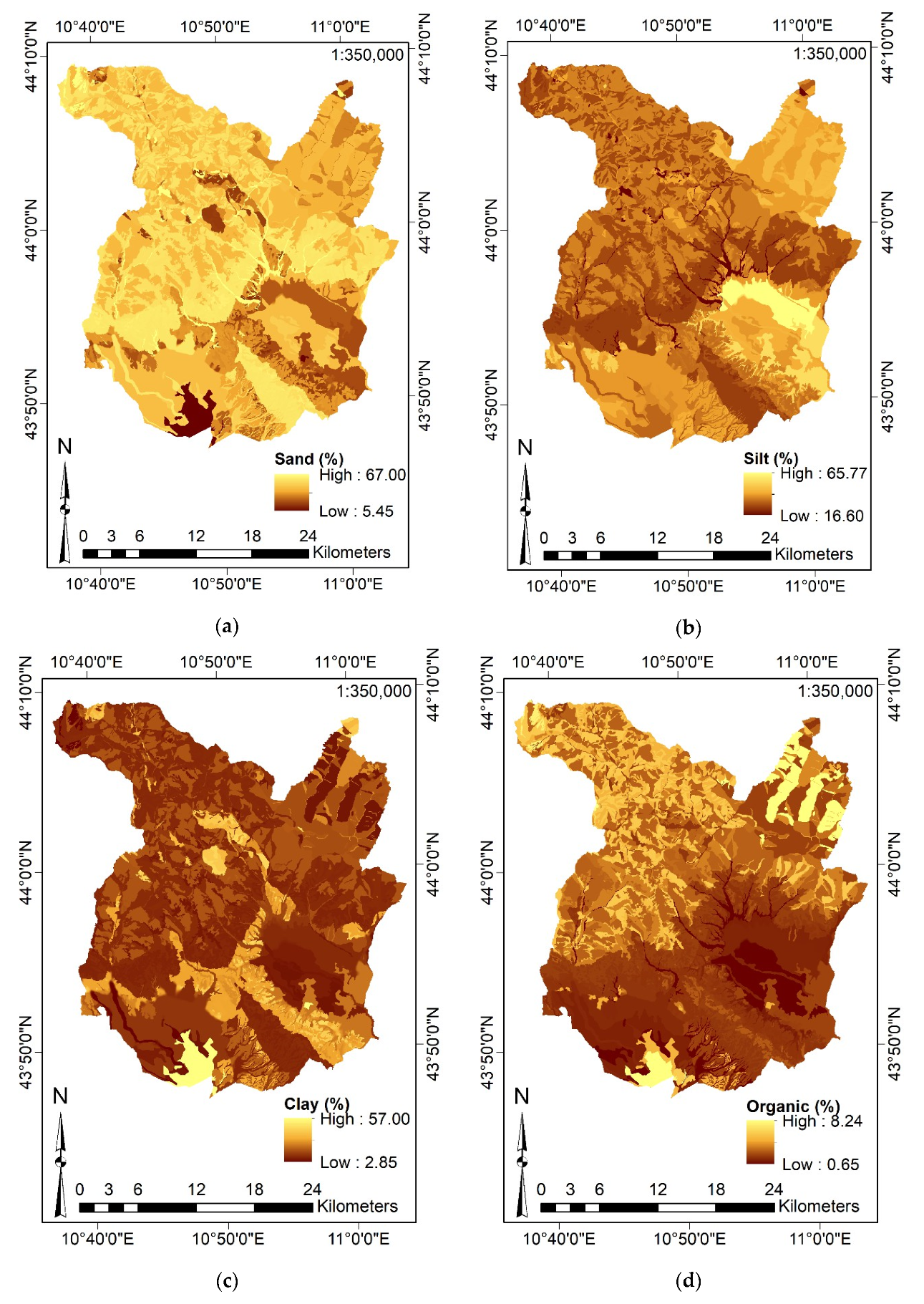
| Content of Sand of the subsoil | [%] | 6.60 | 67.00 | 37.53 | 12.44 | 0.09 | −0.61 | |
| Content of Silt of the subsoil | [%] | 16.60 | 65.36 | 45.59 | 10.44 | 0.10 | 0.56 | |
| Content of Clay of the subsoil | [%] | 2.85 | 51.58 | 16.91 | 7.03 | 1.41 | 1.70 | |
| Content of Organic of the subsoil | [%] | 0.65 | 8.24 | 1.45 | 0.72 | 3.34 | 19.88 |
| Input Feature | Type | Number of Categories |
|---|---|---|
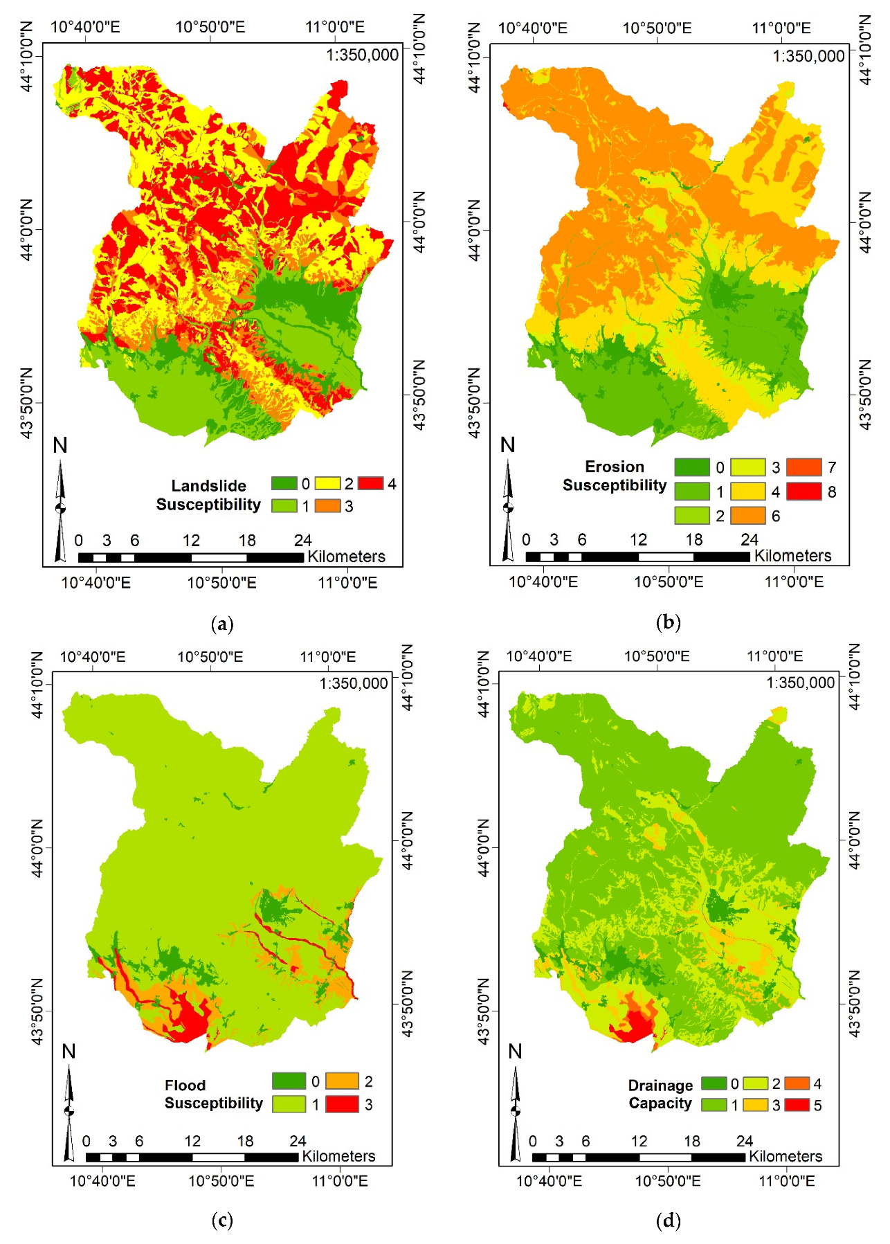
| Drainage Capacity of the soil | Ord | 6 |
| Flood susceptibility | Ord | 4 |
| Erosion susceptibility | Ord | 7 |
| Landslide susceptibility | Ord | 5 |
| Land Use | Cat | 39 |
| Area Type | Bin | 2 |
| Wrapper Feature Selection Approaches | |||
|---|---|---|---|
| Wrapper Type | Forward Feature Selection | Backward Feature Selection | Bi-Directional Feature Selection |
| Selected Attributes | Elevation | Elevation | Elevation |
| Rainfall | Rainfall | Rainfall | |
| Distance from rivers | Distance from rivers | Distance from rivers | |
| Distance from landslides | Distance from landslides | Distance from landslides | |
| Earthquake susceptibility | Earthquake susceptibility | Earthquake susceptibility | |
| Type of area | Type of area | Type of area | |
| River density | River density | River density | |
| Silt content | Silt content | Silt content | |
| Sand content | Clay content | Sand content | |
| Org content | |||
| Starting set | No attributes | All attributes | No Attributes |
| Iterations | 338 | 424 | 464 |
| RMSE | 0.393 | 0.390 | 0.391 |
| Single Learners | ||||
|---|---|---|---|---|
| RT | SVM | |||
| Training | Testing | Training | Testing | |
| St. Dev. [mm/year] | 2.0324 | 2.0173 | 2.0360 | 2.0504 |
| R2 | 0.9766 | 0.9012 | 0.9879 | 0.9500 |
| RMSE | 0.3146 | 0.6570 | 0.2266 | 0.4672 |
| MAE | 0.1664 | 0.3470 | 0.0937 | 0.2658 |
| Ensemble Learners | ||||
| BRT | RF | |||
| Training | Testing | Training | Testing | |
| St. Dev. [mm/year] | 2.0534 | 2.0145 | 1.9777 | 1.9555 |
| R2 | 0.9998 | 0.9557 | 0.9828 | 0.9466 |
| RMSE | 0.0302 | 0.4401 | 0.2694 | 0.4829 |
| MAE | 0.0161 | 0.2641 | 0.1572 | 0.2823 |
| Input Features | Predictor Importance | Forward Wrapper | Backward Wrapper | Bi-Directional Wrapper |
|---|---|---|---|---|
| Organic Content | 70.23 | ✓ | ||
| Clay content | 43.86 | ✓ | ||
| Flood Susceptibility | 41.4 | |||
| Silt Content | 41.29 | ✓ | ✓ | ✓ |
| Distance from Landslides | 37.32 | ✓ | ✓ | ✓ |
| Earthquake Susceptibility | 35.12 | ✓ | ✓ | ✓ |
| Drainage Capacity | 34.34 | |||
| Landslide Susceptibility | 27.8 | |||
| Erosion Susceptibility | 26.24 | |||
| Rainfall | 22.48 | ✓ | ✓ | ✓ |
| Sand Content | 20.37 | ✓ | ✓ | |
| Diffusive Solar Radiation | 19.01 | |||
| Land Use | 18.83 | |||
| River Density | 12.01 | ✓ | ✓ | ✓ |
| Elevation | 11.08 | ✓ | ✓ | ✓ |
| Type of Area | 9.63 | ✓ | ✓ | ✓ |
| Distance from Rivers | 8.17 | ✓ | ✓ | ✓ |
| WE | 7.77 | |||
| TRI | 4.89 | |||
| Direct Solar Radiation | 3.7 | |||
| Slope | 3.37 | |||
| VTR | 3.31 | |||
| Aspect | 2.81 | |||
| SPI | 2.27 | |||
| TWI | 1.88 | |||
| TPI | 1.81 | |||
| Slope Length | 1.72 | |||
| Curvature | 1.28 | |||
| CI | 1.19 |
| Single Learners | ||||
|---|---|---|---|---|
| RT | SVM | |||
| Training | Testing | Training | Testing | |
| St. Dev. [mm/year] | 2.0326 | 1.9794 | 0.6273 | 0.61107 |
| R2 | 0.9162 | 0.8335 | 0.2835 | 0.2625 |
| RMSE | 0.5956 | 0.8448 | 1.7531 | 1.7733 |
| MAE | 0.3747 | 0.5165 | 0.9532 | 0.9652 |
| Ensemble Learners | ||||
| BRT | RF | |||
| Training | Testing | Training | Testing | |
| St. Dev. [mm/year] | 1.9972 | 1.889 | 1.8945 | 1.8078 |
| R2 | 0.9850 | 0.8987 | 0.9724 | 0.8709 |
| RMSE | 0.2524 | 0.6583 | 0.3351 | 0.7499 |
| MAE | 0.1868 | 0.3940 | 0.1937 | 0.4037 |
Publisher’s Note: MDPI stays neutral with regard to jurisdictional claims in published maps and institutional affiliations. |
© 2020 by the authors. Licensee MDPI, Basel, Switzerland. This article is an open access article distributed under the terms and conditions of the Creative Commons Attribution (CC BY) license (http://creativecommons.org/licenses/by/4.0/).
Share and Cite
Fiorentini, N.; Maboudi, M.; Leandri, P.; Losa, M.; Gerke, M. Surface Motion Prediction and Mapping for Road Infrastructures Management by PS-InSAR Measurements and Machine Learning Algorithms. Remote Sens. 2020, 12, 3976. https://doi.org/10.3390/rs12233976
Fiorentini N, Maboudi M, Leandri P, Losa M, Gerke M. Surface Motion Prediction and Mapping for Road Infrastructures Management by PS-InSAR Measurements and Machine Learning Algorithms. Remote Sensing. 2020; 12(23):3976. https://doi.org/10.3390/rs12233976
Chicago/Turabian StyleFiorentini, Nicholas, Mehdi Maboudi, Pietro Leandri, Massimo Losa, and Markus Gerke. 2020. "Surface Motion Prediction and Mapping for Road Infrastructures Management by PS-InSAR Measurements and Machine Learning Algorithms" Remote Sensing 12, no. 23: 3976. https://doi.org/10.3390/rs12233976