Article

DoMars16k: A Diverse Dataset for Weakly Supervised Geomorphologic Analysis on Mars

Image Analysis Group, TU Dortmund University, 44227 Dortmund, Germany
*
Author to whom correspondence should be addressed.
These authors contributed equally to this work.
Remote Sens. 2020, 12(23), 3981; https://doi.org/10.3390/rs12233981
Submission received: 30 September 2020 / Revised: 26 November 2020 / Accepted: 1 December 2020 / Published: 4 December 2020
(This article belongs to the Special Issue Planetary 3D Mapping, Remote Sensing and Machine Learning)

Abstract

:
Mapping planetary surfaces is an intricate task that forms the basis for many geologic, geomorphologic, and geographic studies of planetary bodies. In this work, we present a method to automate a specific type of planetary mapping, geomorphic mapping, taking machine learning as a basis. Additionally, we introduce a novel dataset, termed DoMars16k, which contains 16,150 samples of fifteen different landforms commonly found on the Martian surface. We use a convolutional neural network to establish a relation between Mars Reconnaissance Orbiter Context Camera images and the landforms of the dataset. Afterwards, we employ a sliding-window approach in conjunction with a Markov Random field smoothing to create maps in a weakly supervised fashion. Finally, we provide encouraging results and carry out automated geomorphological analyses of Jezero crater, the Mars2020 landing site, and Oxia Planum, the prospective ExoMars landing site.

Graphical Abstract

1. Introduction

Mapping planetary surfaces is an essential step during future mission planning. It consists, among others, in outlining geological units of the surface and providing a geomorphic and stratigraphic analysis [1]. Mapping is also important when selecting homogenous regions for crater frequency analysis, the search for sampling locations, understanding the global geologic setting, or the different landforms present in a region. It is estimated in [1] to last 5 to 7 years per high quality USGS mapping project, where each project costs around $ 250 , 000 in human labour. While certainly not all mapping projects last that long and are that expensive, creating maps is a tedious and time consuming task. A geological map is built by an expert or a group of experts by manually drawing the outlines of geological units. The experts use geographic information system (GIS) applications, such as ArcGIS, to combine information from different sources, such as different sensors, previous maps, and their experience, to distill it into a single map, which answers the desired science questions.
If looked at through the eye of a computer scientist, creating geologic maps appears to be similar to a common computer vision task: image segmentation. In image segmentation an image is divided into a set of mutually exclusive regions where each region has specific features, such as colour, texture, or semantics. The regions or units of geological maps share geological properties. If we find a way to link the sensory outputs, such as remotely sensed images, which are also used by the experts to build maps, to the geologic properties, we could use the rich image segmentation literature to build an automated system, which can generate maps from image data. However, geologic mapping is challenging. It requires an in-depth knowledge of a planetary body and requires the interpretation and synthesis of multiple cues. Therefore, we focus on geomorphic mapping, i.e., the description of the morphology of landforms observable from orbital images [2], in this work. In contrast to geologic mapping geomorphic mapping does not necessarily reveal information about the stratigraphy of an area [2]. Geomorphic mapping solely depends on the orbital image data and does not require interpreting or synthesising information. Geomorphic mapping is thus more suited for automated approaches than geologic mapping. However, recognising differently shaped landforms poses already a reasonable challenge for automated approaches.
In this work we tackle this challenge and explore a possible approach towards automated landform mapping where we focus on the visual appearance rather than on detecting the geological process which formed a structure. We will review the current state of automated landform analysis and describe their limitations in Section 2. In Section 3 we describe a potential link between image data from the Mars Reconnaissance Orbiter’s Context Camera (CTX) [3] with a resolution of 6 m / px and fifteen common landforms on the Martian surface. Furthermore, we present an automated approach which exploits this link by taking machine learning as a basis. In Section 4 we present the results and discuss the implications and limitations in Section 5.

2. Related Work

Automatically detecting topographic features on Mars dates back to the work of [4]. They used elevation data from the Mars Orbiter Laser Altimeter (MOLA) [5] of the Mars Global Surveyor Mission [6] to divide an area into semantically meaningful regions. The study was conducted in an unsupervised fashion where no labels or expert annotations were used to guide the algorithm. Unsupervised techniques benefit from being directly usable for automatically creating a map without costly expert annotations. Nonetheless, this task is especially challenging and the results are often inferior to the results by a supervised approach using expert annotations. Due to the lack of annotations, unsupervised approaches have to divide the data based on similarities between the samples. However, designing a suitable measure of similarity is challenging and the resulting groupings do not necessarily coincide with a grouping a human would expect. Furthermore, in unsupervised learning the number of different classes has to be estimated somehow from the provided data alone, whereas supervised learning can directly use this information from the human annotations. The work by [7] is the first time expert annotations are used. This has several advantages compared to an unsupervised approach. First, the algorithm is now catered more towards a representation a human would expect. For instance, the division of the data into different classes is set by a human and not inferred from data alone. Second, expert annotations make different approaches comparable through classification metrics, such as precision and recall. Third, by sharing expert annotations with other researchers competing methods emerge. This has lead to tremendous progress in image segmentation and image classification in the general computer vision domain. However, the expert annotations used in [7] have not been shared publicly. Ultimately, the original work of [4] led to the creation of a global map for Mars in [8] and has been extended continuously in [7,9]. Table 1 summarises different studies which are concerned with automated geomorphologic analyses and highlights key properties of the studies, such as the used instrument data, the number of classes, the number of samples, the type of annotations used in the study, and their availability. In the following we will discuss the key elements in more detail.
In addition to the previously discussed studies, which aimed at a global description of the landforms through elevation data, image data from the Mars Global Surveyor Mars Orbiter Camera (MOC) [22] have been used in [10,11]. Later, image data from Mars Reconnaisssance Orbiter’s Context Camera (CTX) [3] and from Mars Reconnaisssance’s High Resolution Imaging Science Experiment (HiRISE) [23] have been used. CTX images have been used in [15,18] and HiRISE images have been used in [12,13,14,15,16,17,19,21]. Besides the used instruments two groups of approaches emerge. The first group focusses on classifying some specific Martian landforms, such as dunes [10,11], rootless cones [15], transverse aeolian ridges [13,15], dark slope streaks [14], or jet deposits [21]. The second group does not focus on a single landform, but rather on a set of different landforms. In [17] six classes—crater, bright dune, dark dune, other, and edge—are used. The last two classes do not have a geological meaning but rather describe an arbitrary other class and the no-data parts framing a CTX image. In [19] this dataset has been modified by removing the edge class and by adding the classes: slope streaks, spiders, and Swiss cheese terrain. Notably, both datasets are shared online with the research community. The work presented in [18] used CTX images and contains six different classes mainly found in the south polar regions of Mars. The classes are: spiders, baby spiders, channel network, swiss cheese terrain, craters, and other.
The most similar approach to ours is the work presented in [20]. Their goal is to automatically map a HiRISE image into a set of geologic classes. The classes are divided into four thematic groups—bedrock, non-bedrock, aeolian materials, and boulder fields—and are chosen to reflect the traversability of the Martian surface in the context of rover missions. Each of the thematic groups consists of one to six individual classes. Rover traversability was also studied in [16]. They build on 17 terrain classes, which have been described in [12]. The work presented in [12] is one of the earliest works which adapts the advances in computer vision to the automatic analysis of orbital images.
The studies presented in Table 1 often contain impact landforms, such as craters, as a class. In fact, crater detection is itself a very active field of planetary research. It is commonly applied to estimate the age of geological units from orbital images. In this work crater detection algorithms are excluded from the comparison (cf. Table 1), because it is beyond the scope of this article to give a thorough overview of this active area of research. A recent survey of crater detection algorithms is presented in [24].
Not necessarily all approaches present a map as final result, but rather classify patches or small windows only. While the earliest and mostly unsupervised approaches [4,7,8,25] operated on pixel-level or superpixel-level, the remaining works [10,11,14,15,17,18,19] operated on box-level annotations (cf. Table 1). Figure 1 collates different levels of supervision in the light of Martian surface analysis. In the case of box annotations a whole box receives the same label and not the individual pixels within the box. Thus, directly operating on pixel-level is favourable for creating the most accurate maps.
Deep segmentation networks, such as U-Net [26] or SegNet [27], are used for pixel-level segmentation. However, these networks have a desire for large amounts of training data [28] to learn the complex relations between image data and semantically meaningful classes. Furthermore, they require pixel-level annotations as training data. Not one of the aforementioned datasets offers pixel-level annotations, describes a variety of landforms, and is shared publicly with the research community. Thus, we could either create a pixel-level dataset or search for different approaches which do not require pixel-level annotations but also yield a map as a final result. Creating a pixel-level dataset is error prone if not performed throughly by a domain expert. It is thus very time-consuming and costly (cf. [1]).
The machine learning literature offers an alternative: weak supervision. With the help of this concept it is possible to bypass the need for pixel-level labels to recieve pixel-level predictions. The previously mentioned box-level annotations are one specific type of weak supervision if the box-level annotations are used to create pixel-level class predictions. An overview of weakly supervised image segmentation is presented in [28]. A recent overview of deep learning approaches in remote sensing in general are presented in [29]. Further details of our weakly supervised mapping framework are presented in Section 3.3.

3. Materials and Methods

In this work we choose to analyse image data from the Mars Reconnaissance Orbiter Context camera because it has a high spatial resolution, which allows us to study a multitude of geomorphological questions. Additionally, the coverage of the Martian surface is almost global and it provides a nice complement to the HiRISE datasets found in the literature [14,15,17,19,21]. The presented dataset will be the largest and most diverse dataset of landforms on the Martian surface built on CTX images. The section is structured as follows. Section 3.1 gives a general outline of the landforms which will be used to classify the Martian surface, Section 3.2 describes the created dataset thoroughly, Section 3.3 explains how geomorphologic maps can be computed automatically in a weakly supervised fashion with the help of the created dataset, and Section 3.4 describes the implementation details necessary to reproduce the results presented in this work. The code for reproducing the results and a link to the dataset are available in the supplementary materials.

3.1. Landforms

To build our weakly supervised geomorphologic mapping algorithm, we need to define a dataset from which an automated system can learn the relationship between the observed CTX images and the landforms present in the images. As a first step, appropriate classes need to be defined. We divide the set of common Martian landforms into five thematic groups: “Aeolian Bedforms”, “Topographic Landforms”, “Slope Feature Landforms”, “Impact Landforms”, and “Basic Terrain Landforms”. Each group consists of at least two and at most four classes. The groups were chosen to primarily suit the science goals described in [3] and the description of landforms on Mars given in [30]. Additionally, the “Basic Terrain Landforms” group is introduced to allow for a description of a broad range of landforms on the Martian surface at least in a basic sense. This is a notable difference to prior work (cf. Section 2) which only focussed on detecting some prominent landforms. An overview of the thematic groups and their respective classes are given in Table 2.
The classes and the thematic groups are build to be extendable. For instance, the “Aeolian Bedforms” (see Section 3.1.1) are currently divided into two classes depending on their visual appearance. If researchers are more interested in describing different types of dunes with more detail, as for instance done in [31] or [11], the classes defined in this work can be used as a basis for an extension of the class hierarchy. For instance, the “Aeolian Curved” class can be divided into its containing dune types: barchan, barchanoid, star, and dome. For each of these new and more granular classes image and label pairs need to be added to the original dataset. However, the existing classes can still be used to build a map of the analysed region. Similarly, other thematic groups can be extended depending on the desired mapping results.
Besides their geological origins the classes have been chosen to match the scale of the window size. In general, the detectable landforms depend on the scale on the surface and the scale of the window size. If a small window size is used, craters which are far larger than the window size cannot be detected anymore. However, if the window size is too large, fine slope features, which are of high interest [3], cannot be detected any longer. Consequently, the window size of 200   px × 200   px or 1.2   k m × 1.2   k m equivalently is a design choice which had to be made. It is a trade-off between annotation effort and the granularity of the final mapping. In general, different scales can be incorporated into the training set, although it requires specialised neural network architectures. One approach is presented in the context of Martian surface analysis in [15]. In this work we refrain from implementing multiple scales, because it creates a significant additional labelling effort and has a minor impact on the reachable classification accuracy [15]. In the following sections the five thematic groups and their classes will be described in more detail. If applicable the geological processes governing the formation of the landforms are also discussed.

3.1.1. Aeolian Bedforms

Wind is one agent of landform modification on the Martian surface [30]. The most distinctive examples are dunes. In general, dunes on Mars are divided into complex and simple shapes [30], which follows the terminology for dunes on Earth defined in [32]. While simple dunes are formed by a single wind direction, complex shapes are formed by wind from different directions. However, some simple types, such as Barchan dunes, are formed by a single wind direction but have a rather complex appearance. Likewise some complex types, such as linear dunes, which appear linear in shape are actually formed by opposing wind directions. An extensive overview of different dune types on Mars and their distribution is presented in [31].
For an algorithmic approach it is challenging to deduce complex information, such as the wind direction, from isolated patches without context. Therefore, we employ a dune classification which is based on the visual appearance of a dune or dune field instead of using the established dune classification scheme by [32]. We divide the set of dunes based on their appearance into a linear case termed “Aeolian Straight” and a non-linear case termed “Aeolian Curved”. The former includes aeolian bedforms which form a linear pattern, such as linear dunes or some transverse dunes. Additionally, transverse aeolian ridges and mega-ripples, which are morphologically similar to dunes, are also included in this class if they form linear patterns. The “Aeolian Curved” class includes barchan, barchanoid, star, and dome dunes. Furthermore, transverse dunes, which form a non-linear pattern, are also included in this class. These dune types have more diverse and curved shapes than the dunes in the “Aeolian Straight” class. Examples of both classes are presented in Table 2.

3.1.2. Topographic Landforms

Other landforms on Mars have been formed by water, ice, or erosion and are summarised in the topographic unit which includes the classes “Cliff”, “Ridge”, and “Channel”. Cliffs and ridges occur, among others, in large canyons such as the Valles Marineris (13.9 N, 59.2 W). Due to the fixed scale of the chosen window size, the rims of craters with diameters far greater than the window size also belong to one of the two aforementioned classes, because partial views of the crater rim look such as cliffs or ridges if viewed in isolation. Depending on the slopes at the crater rim they are either assigned to “Cliff” or “Ridge”.
Outflow channels and valleys are typical landforms which have been formed by water [30]. While some channel-like parts of valley networks fit at least partially into the window size, especially outflow channels are typically larger in their entirety. However, the distinctive layered or streamlined structure present in outflow channels can be recognised without the context provided by the surroundings. The “Channel” class is thus composed of individual flow channels and streamlined parts. Often, dunes are present in individual flow channels [30]. If the dune field at the valley floor is smaller than the window size and the channel-like structure is the dominant feature, the windows are treated as part of the “Channel” class. Otherwise, the dune field is assigned to one of the “Aeolian Bedforms”.
Additionally, small elevated structures, which are round, isolated, have diameters less than 1 k m , and commonly appear in groups, are summarised in the “Mounds” class. Mounds may have been created by a variety of geological processes. The “Mounds” class includes, among others, rootless cones (see e.g., [33]) which have a volcanic origin [34]. Samples of all classes are presented in Table 2.

3.1.3. Slope Feature Landforms

On the Martian surface some features only occur at steep slopes of craters and valleys. In this work, we distinguish “Slope Streaks”, “Gullies”, and “Mass Wasting”. Gullies are mainly found in mid- and high latitudes on both hemispheres [35]. They are several meters wide, around 100 m long [30], and usually consist of three parts: an alcove at the top, an apron at the bottom, and a channel connecting both [36]. As observed in [35] the alcove, the apron, or both may be missing occasionally.
Dark slope streaks are similar in size and commonly occur in equatorial latitudes [37]. They are elongated avalanche-like features which have a lower albedo than their surroundings. Fresh slope streaks are dark, become lighter, and eventually merge with the background. The physical process which steers the formation of both gullies and dark slope streaks remains unresolved [35,37].
Mass wasting is another process which creates commonly observed slope feature. The “Mass Wasting” class consists of image parts where deposits are revealed through loose material sliding down the slope of the surface. The trace of the slipping is visible and it is comparable to slope streaks but lacks the characteristic fan-like structure and strong albedo change. Mature slope streaks with a barely recognisable change in albedo are thus assigned to the “Mass Wasting” class. Examples are presented in Table 2.

3.1.4. Impact Landforms

Craters are an abundant feature on the Martian surface, as on nearly all solid planetary bodies which which have not undergone excessive resurfacing or exhibit active plate tectonics, such as Earth [30]. Depending on the diameter of the crater different forms are distinguished. Complex craters have diameters above 5 to 8 km, and simple craters typically have diameters below 5 km [30]. Due to the fixed window size of 1.2 km × 1.2 km, complex craters are not directly considered to be a separate class, because only partial views of a complex crater fit into the window size. However, the rims of craters with diameters above 1.2 k m are assigned either to “Cliff” or “Ridge” depending on the slope shape at the crater rim. Often, dune fields are found at the crater floor and many of the slope features described in the previous section can be found at the crater walls. Therefore large complex craters are modelled in their entirety by multiple classes.
Craters with diameters less than the window size are classified into a “Crater” and a “Crater Field” class. The former hosts one dominant crater and the latter is used when multiple smaller craters are found within the window. Please note that the radius and the centre of the crater are not part of the annotation. The image-level labels are used as a complementary class to distinguish between different landforms, rather than estimating the properties of a crater. Examples of the impact classes are presented in Table 2.

3.1.5. Basic Terrain Landforms
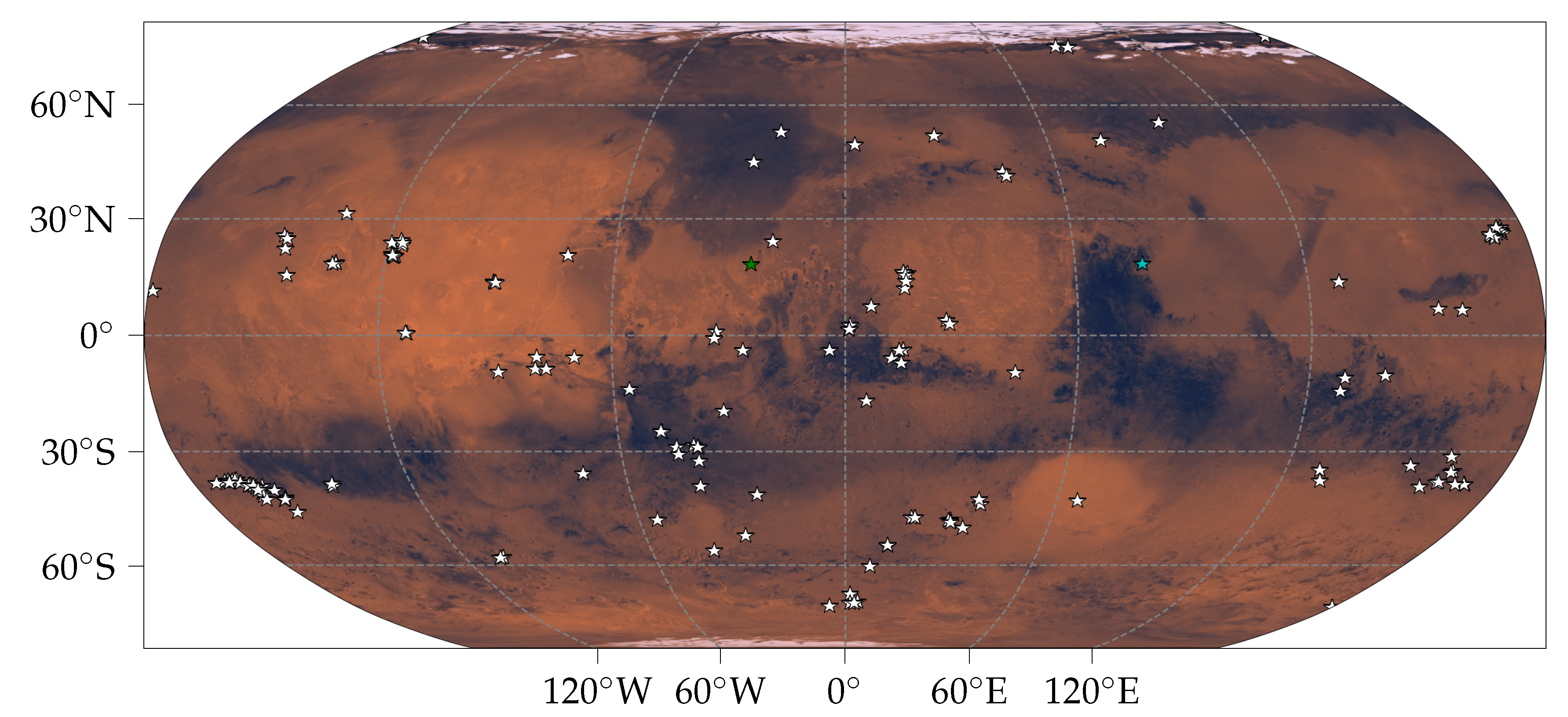
The major goal of this work is to provide a diverse dataset which covers a broad variety of potentially occurring landforms. So far, four thematic groups have been introduced which describe distinctive features on the surface. However, great parts of Mars are covered by bedrock, dust, or both and do not match any of the aforementioned classes. Instead of defining one “Other” class as, for instance, in [17] or one “Negative” class as, for instance, in [15], we introduce a set of four basic terrain landforms. The classes are termed “Smooth Terrain”, “Textured Terrain”, “Rough Terrain”, and “Mixed Terrain”. These four classes represent the basic texture of a landform.
The “Smooth Terrain” class is used for all kinds of smooth surfaces on Mars. It is described in [38] as plain surfaces which are potentially young due to their lack of impact craters. The geological processes creating a smooth surface are, according to [38], lava flows [39], sand [40], or aeolian erosion [41]. Additionally, strong winds and dust storms are observed on Mars [30] which also result in a temporarily smoothed view of the landforms. The “Smooth Terrain” class thus covers all images where bedrock is covered by dust, sand, or other non bedrock materials and no structure is visible. This class comes in various albedos depending on the reflectance properties of the smooth materials.
The opposite of the “Smooth Terrain” class” is the “Rough Terrain” class. It consists of images with sharp patterns induced by steep changes in local slopes. They are numerous in form, spatial frequency, and shape.
Besides the extremes of rough and smooth texture, two mixture classes are defined: “Textured Terrain” and “Mixed Terrain”. The “Mixed Terrain” class contains images with a mixture of smooth and rough terrain. For instance, when bedrock is partially obliqued by dust or smooth and rough bedrock alternate. This class is also important at boundary regions between smooth and textured terrains. It also includes hummocky terrain commonly observed on crater floors or on crater ejecta [42].
The “Textured Terrain” class is used when parts of the bedrock are covered by loose material but the underlying bedrock structure is not completely buried and remains partially visible. This commonly happens in slight dust storms or on slopes where not enough material is present to fully cover the bedrock structure. The “Textured Terrain” class also comes in various forms and shapes. Examples of all classes are presented in Table 2.

3.2. DoMars16k

The dataset presented in this work, which is named DoMars16k, has been created by four human annotators by manually cropping small cutouts containing the described classes from CTX images. In total 163 CTX images contributed with at least three and at most 1247 patches to the creation of the dataset. The final dataset consists of 16,150 samples, which are randomly subdivided into a training, validation, and test set. The training set consists of seventy percent, the validation set of twenty percent, and the test set of ten percent of all samples. The sets are mutually exclusive. The CTX images which have been used to create the dataset have not been selected for specific reasons except for containing the relevant Martian landforms. Other CTX images could have been selected in their stead. Therefore, the dataset can be extended easily in the future.
Each sample has a window size of 200   px × 200   px or 1.2   k m × 1.2   k m equivalently. The window size serves as a trade-off between the landforms present in the window, the annotation effort, and the achievable mapping resolution. The last aspect will be explained in further detail in Section 3.3. In total the 16,150 collected samples cover an area of
16 , 150 × 200   px × 6 m px 2 = 23 , 256   km 2 ,
assuming a constant resolution of 6 m / px [3]. In comparison to the total Martian surface this amounts to a labelled area of 0.0002 %. Or alternatively, we use landforms from 0.001 % of the 113,763 CTX images archived on the Planetary Data System (PDS), which are currently searchable with the Mars Image Explorer (http://viewer.mars.asu.edu/viewer/ctx, Retrieved: 4 December 2020).While these amounts appear small on a first glimpse, the results of our weakly supervised approach presented in Section 4 are already promising.
Figure 2 provides an overview of the CTX images’ locations on the Martian surface, which were used to create the dataset. Please note that not all of the thirty quadrangles were used to sample a CTX image when the dataset was created. These regions are thus especially well suited to study how well an automated system trained on the dataset is able to generalise to unseen data. For instance, the Jezero crater—the landing site of the Mars2020 Perseverance rover—lies in the Syrtis Major quadrangle, which is not covered by training samples. We use the region around the landing site to automatically analyse the geomorphology with our proposed approach to study how well the trained system generalises to unseen data. See Section 4.3.1 for further details. The list of all CTX images which were used to create DoMars16k are listed in Appendix B.

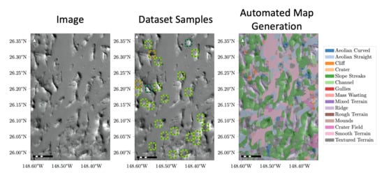
3.3. Automated Map Generation

After introducing the dataset, we present our automated mapping framework. It consists of three steps which are explained in the following sections:

3.3.1. Neural Networks

Neural networks underwent a renaissance roughly ten years ago and are now regarded as the state of the art for classifying large amounts of image data (see, e.g., [29]). The acquisition of CTX images began in 2006 and continues today, but this dataset has not received the same attention from the computer vision community compared to other, commercially more exploitable databases, such as ImageNet [44]. This lack of attention can partially be attributed to the lack of publicly available datasets of annotated Martian landforms. The dataset described in the previous section fills this gap.
Figure 3 depicts an illustration of a typical deep convolutional neural network (CNN) architecture—a VGG-16 [45]. A CNN is composed of different layers, where different layers serve different purposes. CNNs for image classification usually consist of a feature extraction part and a classifier part. In the feature extraction part (green) each layer, such as for instance “conv1”, consists of three different operations: filter blocks (light green), non-linearities (medium green), and a pooling operation (dark green). Each layer may contain multiple filter blocks (here up to three) and each filter block consists of multiple filters (here up to 512). A filter is represented by a matrix and the entries of those matrices are also known as filter weights or simply weights. By convolving the input image with the filters of the different layers and applying the non-linearities and pooling operations, a novel representation of the image is computed at the end of the feature extraction part. The result of these operations is a vector which is also termed an embedding of the image data, because the image is transformed from the space of all images to a lower dimensional representation. This embedding is then fed to a fully connected neural network—the classifier (blue)—for class determination. Here, the classifier consists of three fully connected layers (“fc6”,“fc7”, “fc8”) where each fully connected layer has a fixed number of trainable weights which are again followed by non-linearities. After computing the output of the last layer (“fc8”), a softmax is applied and the output is transformed to a probability simplex, such that the outputs can be interpreted as probabilities. The final class assignment is then achieved by assigning the image to the class with the highest probability. Formally, the softmax (see Equation (2)) transforms the output of “fc8” z = ( z 1 , , z K ) , with K as the number of classes, onto a probability simplex where the individual entries are from the interval ( 0 , 1 ) and additionally add to one.
p ( k i ) = exp z j k = 1 K exp z c
The set of all trainable weights of the feature extraction part and the classifier part are termed the parameters of the network. Adapting the parameters of the neural network is also known as learning and is achieved by minimising a cost function. The cost function used in this work is presented in Section 3.4. Additional details about CNNs in general can, among others, be found in [46] and in the context of remote sensing in [29,47]
We want to examine how well Martian surface analysis profits from the advances in deep learning. Therefore, we use the following widely used CNN architectures as image classifiers: AlexNet [48], VGG [45], ResNet [49], and DenseNet [50]. They have been chosen to reflect the progress in deep learning in recent years. The specific networks mainly differ in design choices such as the number, type and arrangement of layers, and how a signal flows through the network. These differences have been well explained in [29] for a remote sensing audience.
In this work we discuss three different approaches for training a deep neural network on our new dataset DoMars16k. The standard approach for training a neural network from scratch is compared to two approaches which are more beneficial if the number of training samples is limited—transfer learning and pre-training. To train a neural network from scratch, the parameters of a neural network are initialised randomly and then updated during training. After training, the network will be maximally adapted to the training dataset, eventually leading to an over adaptation in the case of smaller datasets.
Transfer learning is an alternative approach, which has successfully been applied to many remote sensing problems on Earth such as [51,52]. The main motivation behind transfer learning is to prevent the CNN from over adapting itself to the limited number of training samples. Hence, a neural network is trained on another potentially very large dataset first. Often, ImageNet [44] is chosen. It consists of roughly 1,500,000 images divided into 1000 classes, such as “Ladybug” or “Foreland”. In the following, we will refer to this type of images as the domain of natural images. Images in this domain depict objects and scenes observed on Earth from an everyday perspective. The domain of orbital Martian surfaces images, which was used to create DoMars16k, is fundamentally different, most obvious through the change from a frontal view in the natural domain to a top-down perspective in the orbital domain.
If a network is trained on a large volume of image data such as ImageNet, it is supposed to be well adapted to a variety of images and has eventually established general purpose features in the feature extraction part. In the second step of transfer learning, the feature extraction layers of the neural networks are frozen and only the classifier part, which assigns the labels to the samples, is re-trained, with the dataset of interest. In our scenario, we train a CNN with the help of ImageNet first and then re-train the classifier part of the CNN on the Martian landforms contained in DoMars16k while keeping the feature extraction part as is. The trained network is thus adapted to the new dataset with limited training effort. Transfer learning can be seen as a low-cost way to adapt the domain of natural images to the domain of interest and is often used when a large training set is not available or costly to come by. In this scenario the parameter-rich neural networks are less likely to overfit on the limited training data and, therefore, tend to generalise better. Further details about transfer learning in general are presented in [53]. In the context of Martian surface analysis, transfer learning has been successfully applied for change detection in [54] and for surface classification in [17].
When using pre-training, the network is also trained on a different dataset first, and instead of fixing the feature extraction part, all layers will be updated during training. Transfer-learning is thus faster than pre-training alone, because only a subset of the large number of parameters has to be updated, which can prevent overfitting as there are fewer parameters to adapt. However, the embedding computed from the images is fixed and does not adapt itself to the domain of the target images. Transfer learning thus works very well if the pre-training domain and the target domain highly overlap. In the context of remote sensing this is not the case and it is difficult to justify in general why transfer learning works when pre-training on ImageNet. In Section 5 we discuss this aspect in more detail based on our results in Section 4.

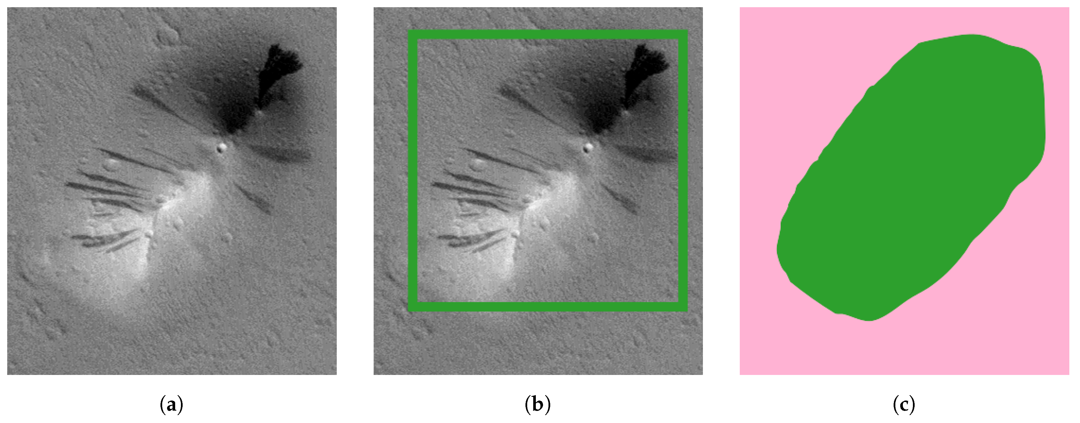
3.3.2. Window Classifier

When creating a map from box level annotations, a weakly supervised approach is necessary (see Section 2). In this work we reinterpret the sliding window as a weakly supervised segmentation approach. The window classifier is a decade old technique which is used, among others, in the “classical” computer vision pipeline for object or face detection [55]. Using a window classifier for weakly supervised segmentation has already been studied in [56] in the context of cloud detection or in [20] in the context of Martian surface traversability (see Section 2).
In general, the classifier—a neural network in our case—does not provide a pixel-level prediction from the input window, but only one prediction for the whole window. This limitation is a result of the training data which just provides one annotation fot the whole window as well. However, by sliding a window over a CTX image the landforms can be localised again and a map can be constructed. The limitation of the window classifier is the window size itself which smoothes the boundary between neighbouring classes, even if the classification is perfect. Figure 4 illustrates this issue. The pixel-level annotation features sharp edges. While this might not be the most common region boundary for landforms, we use this extreme case to illustrate the issue where it is most severe. After classifying the corresponding image with the help of the sliding window approach a smoothing effect at the boundaries is observed. A window always sees several pixels at once when making a decision, in our scenario 200   px × 200   px . Windows which contain more than one class, for instance at class boundaries, are then the cause of the issue. Ideally, the classifier always chooses the class with the largest support in a window. However, in practice this is seldom the case and noisy classifications around region borders are observed. In this work we try to improve this behaviour by filtering the predictions accordingly. See Section 3.3.3 for additional details on the filtering. Additionally, a window classifier creates a large computational overhead because every pixel is seen multiple times.
When sliding the window classifier over the image, every pixel of the analysed region—a CTX image for instance—receives a prediction. However, not all windows contain a distinctive feature, such as a crater. Therefore, it is crucial to have the basic terrain classes defined in Section 3.1.5 as classes in order to ensure a meaningful mapping. Otherwise, windows might be assigned to any of the other classes irrespective of how well the embedding of the window matches the distribution of the classes. The reason for this behaviour is the softmax function (see Equation (2)). Due to the overconfidence commonly observed in deep neural networks [57] almost always one class alone will have a high membership probability leading to uncalibrated estimates of the class memberships. Further details are presented in Section 4.

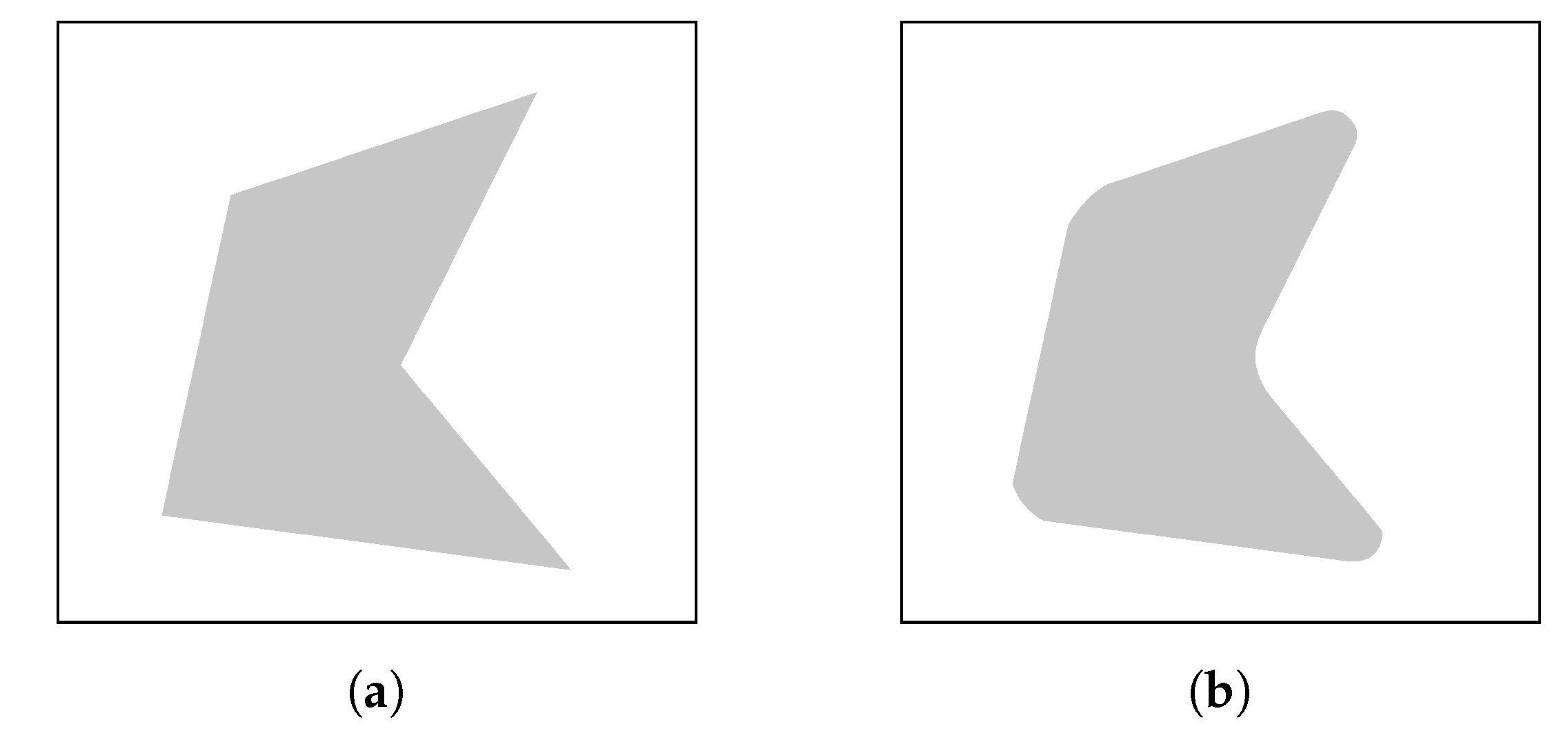
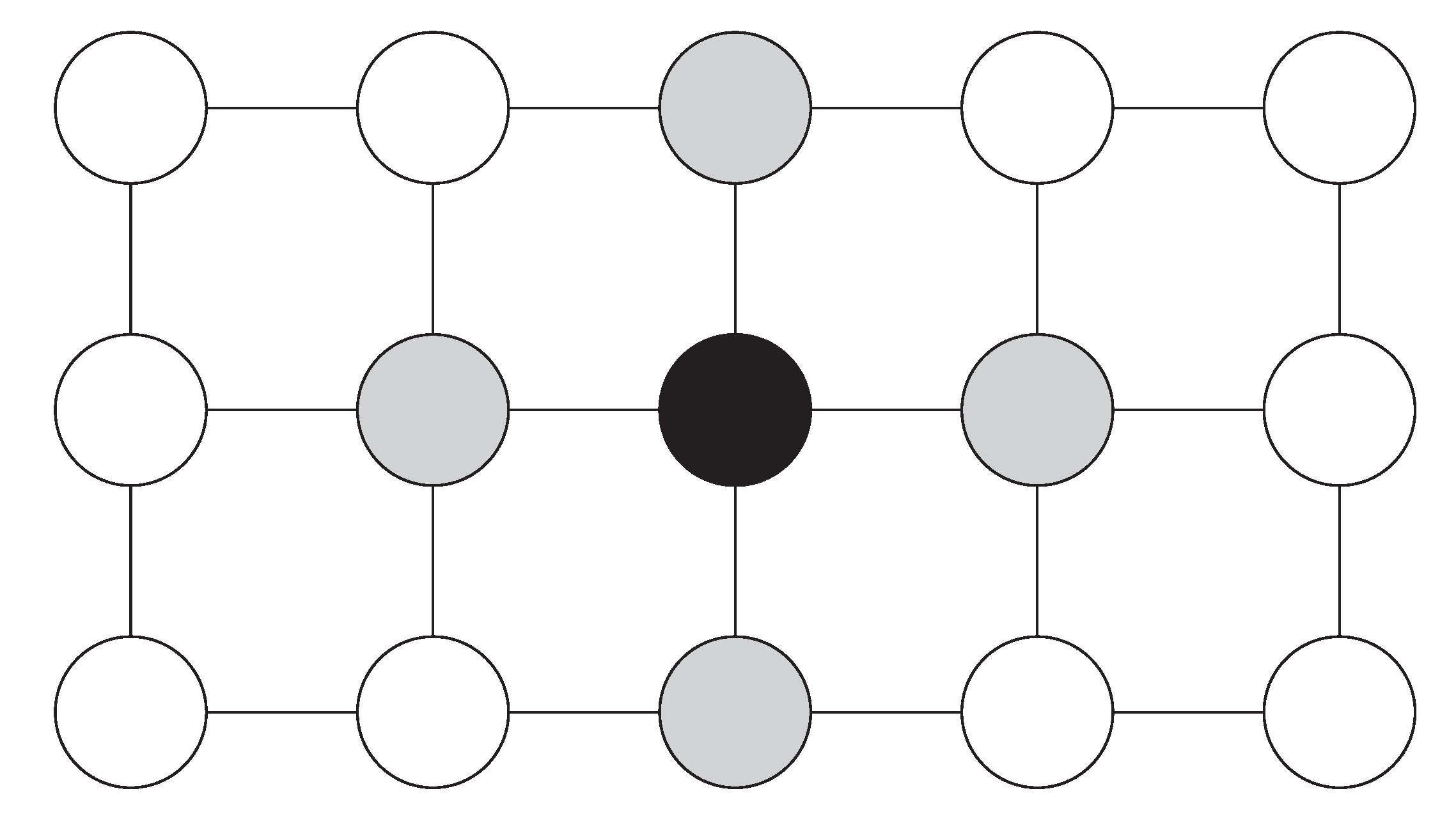
3.3.3. Markov Random Fields

Noisy results can be smoothed to appear more homogenous and thus look more like the mapping a human would create. In this work we use Markov random fields (MRFs) to smooth the outlier corrupted mapping of the sliding window classifier. The window classifier only uses the information contained in a small part of an image for class determination. Therefore small variations in the content of a window can have large impacts on the classification, if the network is overconfident in its prediction, which in turn can lead to outliers in otherwise homogeneous regions. Especially at borders between two different landforms, uncertain classifications lead to this effect. Incidentally, human maps share the same ambiguity when transitioning from one unit to another [2]. While human mappers can base their decision where to draw a unit boundary on their experience and interpretation of the area, the machine makes an isolated decision based on the information available in the current window. In order to reduce outliers and uncertain classification at class borders we employ MRFs as a model for the surroundings of a window. The window size is thus increased artificially in hindsight by smoothing the results.
The MRFs used in this work have two parameters: a neighbourhood correlation γ [ 0 , 1 ] and a neighbourhood size w N + . The neighbourhood parameters γ and w steer how strong the relation between individual pixels and their surroundings are supposed to be. Hence, they control the strength of the smoothing. An MRF is estimated in an iterative fashion. Therefore, the number of iterations r N + is an additional parameter, which has to be set in practice. In this work we use a hard convergence criterion and stop the computation after a fixed number of iterations. Additional details are presented in Appendix A. Results before and after filtering are presented in Section 4.

3.4. Software and Experiment Parameters

Training the neural networks was conducted using the Python programming language (Version 3.8.5), PyTorch 1.6 [58], and Numpy 1.19.1 [59]. Processing the georeferenced CTX images was done with the Geospatial Data Abstraction Library (GDAL) [60] and scikit-image [61]. Numba 0.5 [62] was used for accelerating the MRF computation. Neural network training and inference was accelerated by an NVIDIA RTX 6000 graphics card.
For all analysed network architectures a batch size of 64 was chosen during training. The cross entropy loss was used as a loss function. It is given for N samples with C classes as (see, among others, [63]):
CE ( y , y ^ ) = i = 1 N y i log y ^ i ,
with y i = ( y i , 1 , , y i , C ) as a one-hot-encoding of the ground truth class for the i-th sample, and the vector of predictions y ^ i = ( y ^ i , 1 , , y ^ i , C ) for the i-th sample.
The networks were trained for 30 epochs with stochastic gradient descent (SGD) in the case of pre-training and transfer learning and with Adam [64] in the case of training from scratch. The learning rates were chosen as 0.01 and 0.0001 , respectively. In the case of SGD a momentum of 0.9 was added. The Markov random fields used a neighbourhood correlation of γ = 0.3 , a neighbourhood size of w = 11 , and were estimated with r = 5 repetitions.

4. Results

This section describes the results of the method proposed in this work. First, different neural network architectures are analysed with regard to their ability to learn the link between the CTX images and the landforms with the help of our dataset. Second, we analyse the best performing model and present results of the automated mapping approach, where parts of the map were seen by the neural network during training. Last, based on the encouraging results, we apply our mapping framework to analyse the geomorphology of the final landing site candidates of the ExoMars and Mars2020 rover missions to showcase the capabilities. The landing sites pose the greatest challenge to the automated mapping approach, because the trained neural network has never seen samples from those regions during training (cf. Figure 2). It is the ultimate challenge to study the generalisation potential of our approach.

4.1. Quantitative Accuracy Assessment

In Section 3.3.1 we discussed different approaches to train a deep neural network for image recognition in the light of limited training data. The results of the analysis on our dataset comparing the discussed approaches are presented in Table 3. We report the macro and micro averaged F1-scores (see, for instance, Ref. [65]) as summary metrics. The higher the F1-score the better the performance. The F1-score is defined as a combined measure of precision and recall. Following the notation in [66], precision and recall are comprehensibly introduced through set notation. First, for a binary classification problem and then for the multi-class case applicable in this work.
In a binary classification problem the set of all ground truth labels L can be divided into the set of positives P gt and the set of negatives N gt , such that L is the union of P gt and N gt . Furthermore, we have a corresponding set of predictions V , which contains the set of predicted positives P c and the set of predicted negatives N c by the classifier we want to evaluate. The set of true positives TP is then the intersection of P c and P gt . It describes the set of positive predictions which have also been labelled as positive in the ground truth. The set of false positives FP is the intersection of P c and N gt and contains those elements which are wrongly classified as positive. The set of false negatives FN is the intersection of N c and P gt . It describes the set of negative predictions which are labeled as positive in the ground truth. With these sets, precision and recall are defined as:
precision = | TP | | P c | , recall = | TP | | P gt |
with | · | as the cardinality of a set, i.e., the number of elements in the set. Both measures are easily fooled. For instance, a classifier could receive perfect precision by always predicting the positive class. In order to balance precision and recall, the harmonic mean of the two is often used. It is known as F-measure or simply F 1 and is defined as:
F 1 = 2 precision × recall precision + recall .
In the case of multiple classes, precision and recall are averaged to compute a single metric. There are two approaches possible which are known as macro average and micro average. The macro average computes precision and recall of each class individually and then averages them. Micro averaging computes the necessary sets ( TP , P c , P gt ) for all classes at once and then computes precision and recall from them. Both strategies yield different results and depending on the number of samples in every class, these measures can differ strongly. Our dataset DoMars16k does not suffer from a severe class imbalance (cf. Table 2). As a result, the micro and macro averaged metrics barely differ and yield the same ranking. However, for replicating our results we explicitly state which strategy was used.
In general the examined architectures behave as expected (see Table 3) and similar rankings are observed on other datasets, such as ImageNet [44]. A comparison on ImageNet is, among others, presented in [29]. We can therefore conclude that the created dataset is well balanced and suitable to assess the performance of an automated landform classification. The best performing approach is a DenseNet-161 architecture which is trained with pre-training. Training the same network architecture from scratch severely degrades the performance—a difference in seven percentage points. Using transfer learning degrades the performance even further, yielding a difference of ten percentage points compared to the pre-training approach.
The picture for the remaining architectures is similar with the exception of the AlexNet which we will discuss later. All architectures perform best if they are pre-trained on ImageNet. Apparently, having derived a useful representation of image data prior to learning the relation between landforms and CTX images appears to be beneficial. Although images that depict natural and man-made objects and scenes, as ImageNet does, appear to be very different from orbital images. We discuss potential reasons in Section 5.
When training from scratch the parameter-rich neural networks, such as the ResNet-50, appear to overfit quickly. The results of the pre-training scenario indicate that those networks can perform better if trained differently. However, around 12,000 training images appear to be insufficient to robustly train a network with good generalisation properties from scratch. The DenseNet-121 performs best in this scenario. However, the performance is around four percentage points worse compared to the pre-trained variant. Overall, training from scratch always degrades the performance, from architecture to architecture even severely.
Transfer learning is a common choice to make the best use of a limited amount of training data (see Section 3.3.1). However, transfer learning provides the worst results in our scenario. Only AlexNet benefits from this training strategy, but only in comparison to training from scratch. Thus, it appears as if the relatively simple AlexNet architecture has the most general feature extraction. Recall that the main difference between transfer learning and pre-training is how many parameters are updated during training. Both approaches are initialised with weights from an architecture trained on ImageNet. In our scenario, freezing the feature extraction part to prevent overfitting does more harm than good and prevents the neural network from learning useful representations of the Martian surface data. Albeit the computational overhead, pre-training is clearly the best approach in our scenario.
In order to study the results in more detail Table 4 summarises the metrics class-wise. It is evident that all classes are well classified except “Textured Terrain”. Furthermore, “Cliff” and “Ridge” are slightly worse than the remaining classes. The best performance is achieved for the “Aeolian Bedforms”, the “Impact”, and the “Slope Feature Landforms” with near perfect F1-scores.
In order to analyse the reasons why some classes perform worse than the others we provide a confusion matrix in Table 5. The confusion matrix depicts counts computed on the test-set and shows how often the actual classes are predicted as one of the other classes. For instance, 102 images are assigned to the “Aeolian Straight” class where 99 were correctly classified as “Aeolian Straight”, one was wrongly classified as “Channel”, one was wrongly classified as “Rough Terrain”, and one was wrongly classified as “Textured Terrain”. Ideally, all samples are correctly assigned and the confusion matrix has only values different from zero on its diagonal. The confusion matrix allows us to study in more detail which classes are hard to distinguish.
From Table 5 it becomes evident that “Textured Terrain” is most often confused with the other classes of the “Basic Terrain Landforms”. Recall, the “Basic Terrain Landforms” have been introduced to allow for a description of a broad variety of possible landforms on the Martian Surface. Naturally, the visual variability in this thematic group is the broadest and often no distinctive features may be recognised. Furthermore, the transition between the basic terrain units is less specific than between for instance “Crater” and “Gullies”. These classes have their own specific characteristics which are well captured by the neural network and the “Basic Terrain Landforms” remain challenging. We discuss the implications of this result in more detail in Section 5. Some confusion also appears between “Cliff” and “Ridge”. During labelling this information can often be deduced from the context—the surroundings of the patch—but this information is lacking when presenting the patch to the neural network in isolation. The ambiguity between those classes is best resolved by incorporating depth data and provides an interesting future work direction.
A final remark: through excessive hyper-parameter tuning better results may be possible and the last bit of accuracy may be squeezed out of the data by using more advanced neural networks. However, the observed differences remain small—around five percentage points between the best (DenseNet-161) and the worst model (AlexNet)—and the advances may be solely attributed to a more efficient use of a reduced number of network parameters.

4.2. Qualitative Accuracy Assessment

After successfully validating the performance of the trained network, we take a look at some qualitative results. In Table 6 we present samples from the test set which were misclassified by the best performing network—the DenseNet161 pre-trained on ImageNet. This makes the confusion between the different landforms more tangible and provides a complementary view to the quantitative assessment in the previous section. The table shows at most five misclassified samples per class and at least the total number of misclassifications per class, which amounts to two in the case of “Crater” and “Aeolian Curved”. The total number of misclassifications per class can be derived from the confusion matrix (see Table 5) by summing the off-diagonal elements row-wise. Notably, no test set sample of the “Slope Streaks” class is misclassified. Therefore, it does not appear here. Besides the misclassified samples per class it is also depicted which class is chosen instead of the correct one. For instance, the two misclassified “Crater” samples are mistaken for “Crater Field”, probably because the size of the craters are rather small and this crater size is more often observed in the “Crater Field” class. In this cases the neural network failed to capture that a “Crater Field” consists of more than one crater. Other misclassifications, such as the second example in the “Aeolian Curved” class, can be attributed to the chosen window extents. As previously discussed in Section 4.1 the network views the samples in isolation and is therefore not aware of the surroundings of a given window. However, this information might have helped to correctly identify the given sample as an aeolian bedform. The ambiguity between “Cliff” and “Ridge” is often also difficult to solve when the samples are observed without the context of their surroundings.
In Figure 5 a segment of the western Lycus Sulci region (24.6 N, 141 W) is depicted. Parts of this region were used to create annotations for our dataset. The samples in this image are almost exclusively from the class “Slope Streaks” and one sample belongs to the “Ridge” class. The samples of the training, test, and validation set are shown in the context of their surroundings. The squares are colour-coded with two alternating colours. One colour represents which set the samples belong to. The colours olive, orange, and blue indicate if a sample is from the training, test, or validation set, respectively. Additionally, the squares are also green which indicates that the best-performing network—the DenseNet-161—classified this sample correctly. Notably, all samples of the dataset are correctly classified regardless of the set they come from. Apparently, the network has successfully learned to infer the correct landform for every considered window and generalises this knowledge very well to unseen windows.
After successfully classifying the labelled training samples and the previously unseen test images correctly, we now investigate how well the network performs in the remaining areas of this region. Here we make use of our automated mapping approach (see Section 3.3). Recall that all other possible windows in this region, except the ones shown in Figure 5, are not part of the dataset. The neural network has thus never seen the remaining parts and has to infer a classification from the images of the training set. If the network is well trained it can generalise well and we will observe reasonable classifications across the whole area.
The result is presented in Figure 6. It shows the same region that was previously discussed in the context of the training set. The studied region mainly consists of a smooth surface which is traversed by mountain ridges. At the slopes of the ridges several dark slope streaks are visible. In the smooth regions wind also created barely visible linear aeolian features. Occasionally, a few larger craters are observed and two major crater fields emerge in the south and mid eastern parts of the area. Notably, the network has never seen a crater field or smooth terrain from this specific region, and still it is able to reasonably map the respective landforms in this region. Furthermore, it has only seen twenty-four examples of “Slope Streaks” and one example of “Ridge” from this region. This are only 25 of the 2600 × 3800 = 9,880,000 possible windows or around 0.0003 % equivalently—only a tiny fraction. In addition, our approach is able to generalise well to unseen data and is able to provide a meaningful geomorphological map of the whole area.
Two well classified example regions are also depicted on a smaller scale in the bottom part of Figure 6. The region shown in Figure 6a features a ridge surrounded by smooth terrain with occasional aeolian features in the north. The majority of the ridge’s slopes show dark slope streaks. This is well covered by our map. However, the boundary between the smooth plain and the ridge could be improved. The region shown in Figure 6b is part of a larger ridge which is also surrounded by a smooth plain. Here, the automated approach identified that the top of the ridge partly does not feature dark slope streaks and thus assigned the “Ridge” class to those image parts. The surrounding smooth plain is again well captured by the computed map. This time, the boundary seems to adhere more to the topography of the area compared to the previous example.
Besides the occasional inaccurate boundaries, some more obvious misclassifications are present in the generated map. For instance, areas with larger mounds that are too small to be recognised as “Ridge” are mistakenly assigned to “Aeolian Curved” (cf. Figure 6c). Occasionally, ridges are assigned to the “Cliff” class (cf. Figure 6d). This behaviour was also visible in the confusion matrix depicted in Table 5 and probably depends on how the albedo changes in the window. Additionally, we observe a smoothing effect at region boundaries. The causes for this behaviour were discussed in Section 3.3.2 and an illustration of the issues was presented in Figure 4. As a result, not all landforms are mapped in their entirety. For instance, the mountain ridges traversing the smooth areas are not fully covered but often replaced by the “Slope Streaks” class. Depending on which features are most prevalent for the neural network, the most dominant classes are assigned to the windows (see also Figure 6b). However, the overall picture matches the landforms reasonably well and several mountain ridges are very well mapped by our automated approach. Furthermore, the results have been achieved by training on box-level annotations only (cf. Figure 1). Nonetheless we are able to compute a pixel-level map in this challenging scenario.
So far we have only shown the results after using the full mapping pipeline presented in Section 3.3, which includes the MRF smoothing. To assess the influence of the smoothing, a small area has been visualised before and after MRF filtering. The results are presented in Figure 7. Prior to the filtering a noisy pattern is visible. The pattern reflects the uncertainty of the neural network in boundary regions. The pattern has two causes. First, due to the lack of calibrated predictions—a deep neural network tends to be overconfident—a salt-and-pepper-like noise emerges. Second, due to the sliding window classifier, windows with a mixture of two classes are observed, especially at region boundaries. This further strengthens the salt-and-pepper noise in those regions. In fact mixtures of several landforms are not part of the dataset and are thus never observed during training. Nonetheless the mappings are reasonable and capture the essence of the geological landforms present in the image.
After applying the filtering the map is smoothed as desired and, additionally, the structure of the boundaries is retained. Through the filtering we do not observe an additional smoothing of the region boundaries. Only the smoothing through the sliding window classifier itself. After filtering, the map looks more like a human-created map. Actually, by applying the probabilistic Markov random field filtering, we have incorporated a model for the context of a single window, similar to something a human would do in case of uncertainty.

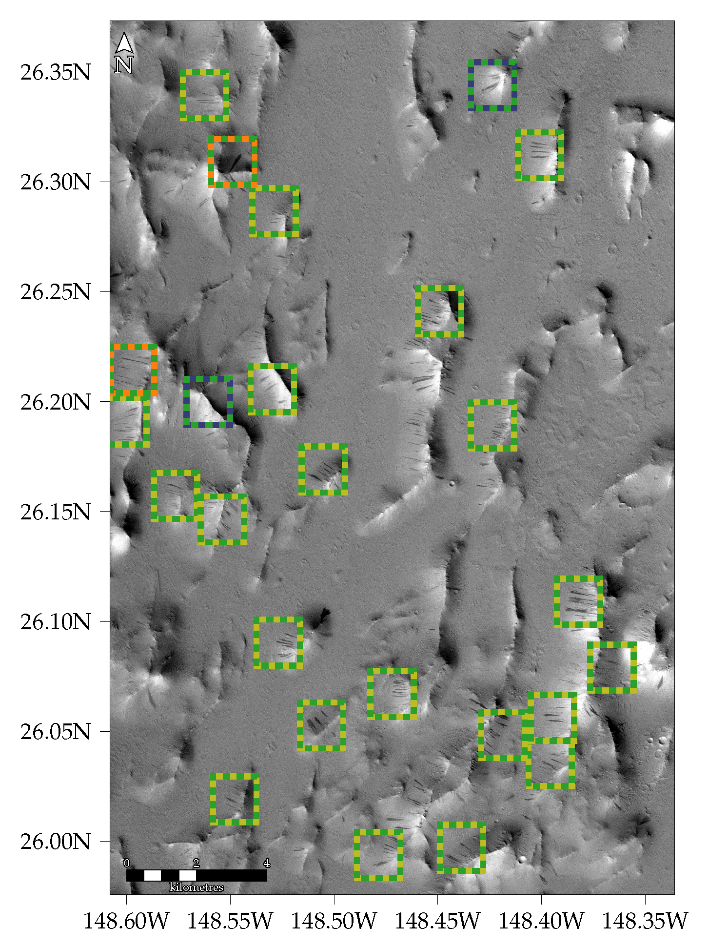
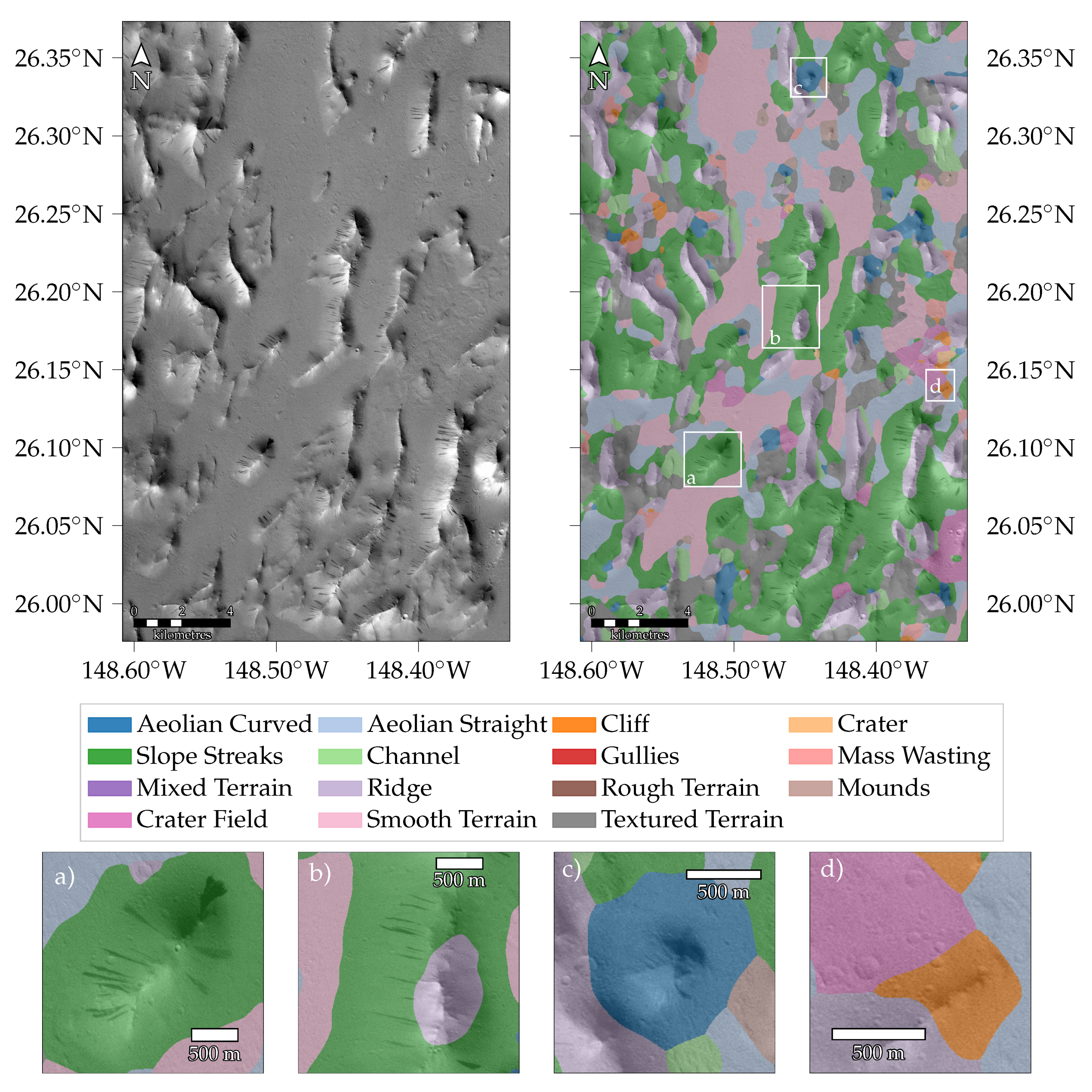
4.3. Landing Site Analysis

Geomorphological maps are, among others, used in the process of landings site determination and planning. In this section we provide maps for the Mars2020 landing site, the Jezero crater (18.38 N, 77.58 E), and the prospective ExoMars landing site, Oxia planum (18.28 N, 335.37 E). Both maps have been generated by our automated approach with the same parameters as discussed in the previous section. No additional training material or anything else adapted specifically to those two regions was used. Our training set did not include any images of Jezero crater or Oxia Planum. Analysing the geomorphology of those regions, is therefore the ultimate challenge for our automated mapping approach.

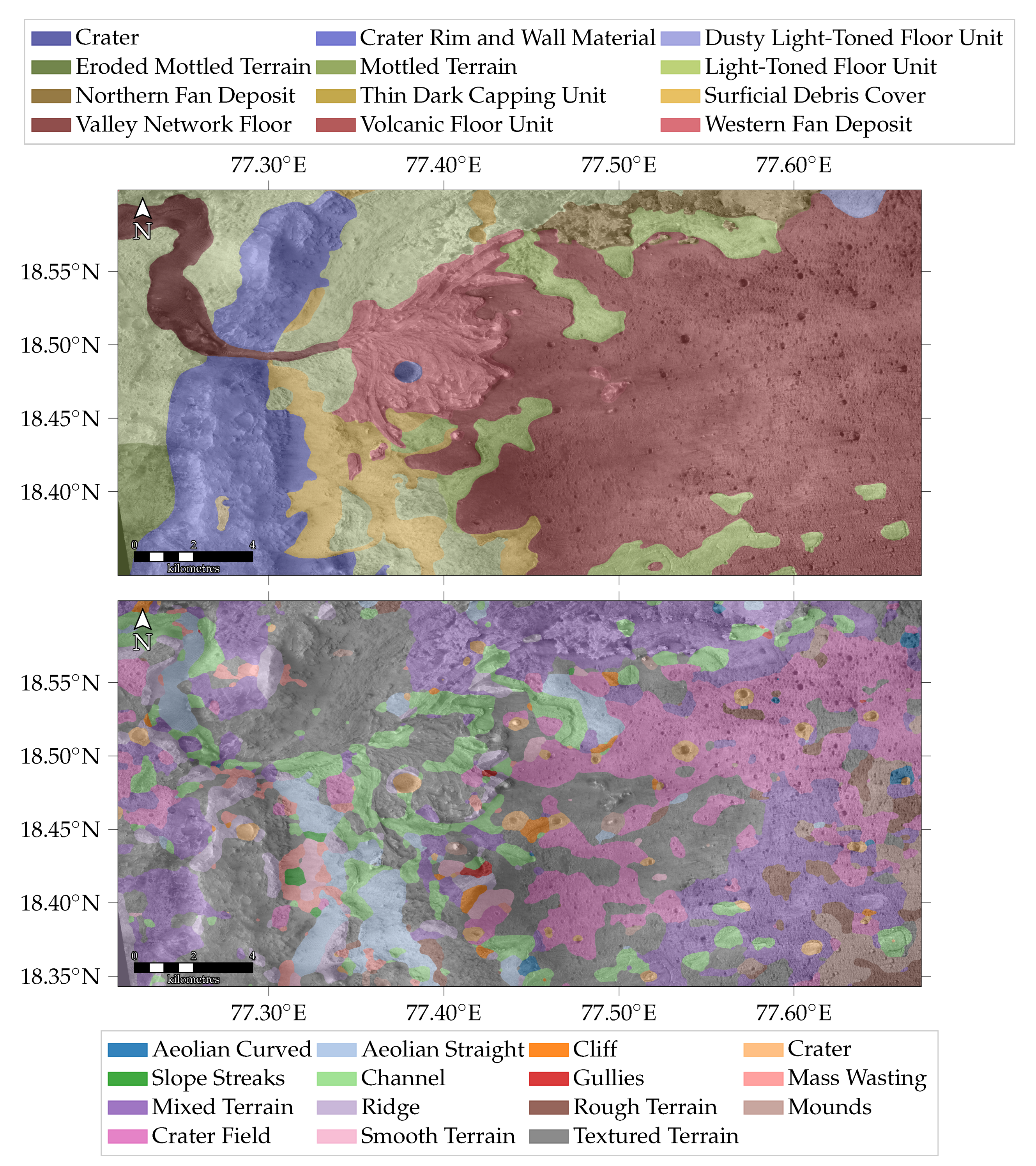
4.3.1. Jezero Crater

Jezero crater has been selected as the landing site of the Perseverance rover of the Mars2020 mission (https://mars.nasa.gov/mars2020/mission/science/landing-site/). The centre of the landing ellipse is located at 18.45 N, 77.46 E. Jezero crater itself is supposed to have hosted an ancient lake connected by a channel system [67,68,69,70]. The most distinctive landform of the area is the delta at the west-side of the crater (see Figure 8). Since the delta is too large to fit into a single window we would expect our automated approach to find a reasonable decomposition of the delta into several classes of the dataset. A reasonable representation would include craters, channels, and a basic terrain landform describing the texture of the bedrock.
The result of the automated mapping is presented in Figure 8. The studied area consists mainly of “Crater Field”, “Channel”, “Aeolian Straight”, a few “Ridges”, some larger “Crater”, and the “Basic Terrain Landforms”. The eastern parts of the map mainly consist of a large crater field in the north and of “Textured Terrain” and “Mixed Terrain” in the south. Especially, the channel, starting in the top left corner and ending in the delta, has been well modelled by the automated approach. Additionally, the large linear dune fields within the channel and south of the delta are well recovered. The abundant craters are, once their size suits the window size, mapped as well. The remaining craters are assigned to the “Crater Field” class.
A few obvious errors are made as well. For instance, this region does not feature gullies and some wind streaks in the eastern parts are confused with “Aeolian Curved”. Although Jezero crater’s dark-toned mafic floor is discussed to have a volcanic origin [71,72], which matches the predicted “Mounds” class in the south-eastern parts, the suspected “Mounds” would be best attributed to the “Rough Terrain” class. Large portions of Figure 8 are assigned to the basic terrain units. While this can be interpreted as a good sign of the validity of the approach and the design of the classes, it shows that there is a need for a more diverse distinction between different types and appearances of bedrock. Another limitation of our approach is visible in the south west corner, where the used CTX image does not contain image data. The neural network used in our automated mapping approach is unaware of such a case and thus simply assigns those pixels to the landform it thinks is most appropriate. Here, “Ridge” is chosen, probably due to the light dark transition often observed on ridges where the topology shades the area in a similar way.
In order to put the map created by the proposed approach in the perspective of maps created by human experts, we can compare ourselves with the maps presented in [73] or [67]. We have chosen the map by [67], because it is publicly available from their website (https://www.jsg.utexas.edu/goudge/shared-data/) for research purposes. The comparison is shown in Figure 9.
The most striking difference between the maps is that our approach does not identify the characteristic delta (“Western Fan Deposit” [67]) in its entirety. The automated approach rather identified individual “Channel”-like structures and attributed the fan deposit as “Textured Terrain”. From the neural network’s perspective this is a sensible classification, because the dataset does not contain a “Deposit” class. This does not render the approach useless but rather requires further processing by a human expert, either by introducing novel classes as suggested in Section 3.1 or by reinterpreting existing classes and merging them accordingly. For instance, the “Valley Network Floor” by [67] is reasonably well recovered by our approach when the corresponding “Channel” and “Aeolian Straight” classes are merged. Here, our approach actually provides additional information and visualises where aeolian bedforms are visible on the valley network floor. The “Crater Rim and Wall Material” segments of [67] are also decomposed into several classes by our approach. Jezero crater is far larger than a CTX image captured at the lowest altitude. It does not even fit into the considered area or let alone the considered window size of 1.2   k m × 1.2   k m . Therefore, the automated approach does not stand a chance to recognise theses parts as a crater rim. As previously discussed in Section 3.3.2, the rim is thus decomposed into several other classes which match the given scale. Here, mostly “Textured Terrain” and “Ridge” are chosen. In Section 3.1.5 we have described “Textured Terrain” as bedrock which is partly covered by loose material. Therefore, the assignment is sensible and matches the look of the crater rim. In contrast to the map by [67] the boundary between “Crater Rim and Wall Material” and “Mottled Terrain” in the northern part is missed and the mottled terrain is—like the crater rim—mostly assigned to “Textured Terrain” by our approach. However, the boundary between “Mottled Terrain” and “Eroded Mottled Terrain” by [67] in the south eastern part is also covered by our automated approach although different classes are chosen. The large “Volcanic Floor Unit” mapped by [67] is decomposed into “Crater”, “Crater Field”, and the “Basic Terrain Landforms” by our approach. The northern part of the “Volcanic Floor Unit” features some craters which match our chosen window size and are therefore mapped individually. The majority of the remaining smaller craters are assigned to the “Crater Field” class. Notably, the “Light-Toned Floor Unit” by [67] is not covered by our approach. Occasionally “Channel” has been chosen but this is a result of a comparable surface gradient at the boundaries to other classes rather than the visual appearance of the class. The greatest resemblance between both maps is the overlap of the “Surficial Debris Cover” class by [67] and the regions which have been attributed to “Aeolian Straight” by our approach.

4.3.2. Oxia Planum

The other region we analyse with our automated mapping approach is Oxia Planum, which is the selected landing site of the rover Rosalind Franklin of the ExoMars programme (http://www.esa.int/Our_Activities/Human_and_Robotic_Exploration/Exploration/ExoMars/Oxia_Planum_favoured_for_ExoMars_surface_mission). The region is most interesting for potentially exhibiting bio-signatures created in the context of liquid water. The area is described as a clay-bearing plain with a fluvio-lacustrine system in which several fluvial morphologies meet [74].
The map created by our automated mapping approach is presented in Figure 10. According to our map the area contains mostly crater fields and a mixture of “Rough Terrain” and “Textured Terrain”. The larger crater in the south-east is too big to fit into a single window and is thus decomposed into several landforms, as with the delta in Jezero crater discussed in the previous section. The crater rim is mapped as “Ridge” and the crater floor as “Aeolian Straight”. Both classes are correct and the crater floor indeed features aeolian ripples, which form a linear pattern. The predicted gullies at the slopes of the crater are debatable, but some sort of material has been sliding down the slope which is correctly detected by the approach, although a suboptimal class was chosen. Additionally, the remains of a channel were correctly identified at the northern parts of the crater rim. The channel originating in the south-eastern corner of the image is also identified correctly. In its vicinity a large dune field is also found. Again, the craters that match the window size are all found confidently and the smaller craters are grouped into the “Crater Field” class. The two darker-toned basins in the north and south-west are decomposed mainly into “Crater field” and one of the “Basic Terrain Landforms”. The south-west basin is part of a degraded crater and has a slightly different geomorphology compared to the northern basin according to our approach. While the latter is mostly a large crater field with occasional dune-like patterns, the former is a rough textured terrain with a few larger craters and smaller crater fields. The remaining light-toned parts are mostly attributed as “Textured Terrain”. Our map can, among others, be compared to the works of [75,76], or [77].
In summary, the overall structure of this region is well covered by our approach. However, a map which adheres more thoroughly to the obvious boundaries between the dark and light-toned areas would be preferable. Therefore, this area would potentially benefit from a more diverse description of different types of bedrock.

5. Discussion

In this work we showed that it is possible to provide an automated geomorphological analysis of the Martian surface in a weakly supervised fashion. The mapping pipeline consists of three major parts: training a classifier, combining it with a sliding window, and an optional filtering.
Using a pre-trained network as initialisation instead of random weights provides an increased performance in our experiments (see Table 3). The difference is up to thirteen percentage points in F-measure, which is a significant gap. This matches the outcomes described in the context of natural scenes [78], medical image analysis [79], and Earth remote-sensing image scene classification [52].
We have also shown that a simple transfer learning protocol yields inferior results on our dataset. The two image domains—natural scenes and orbital Martian surface images—appear to be too different for transfer learning. In general, it could therefore be useful to not only consider transfer-learning or fine-tuning as in [80] or [17], but also use a pre-training approach to improve the results. This might serve as a valuable hint for future work in applying pre-trained networks to remotely sensed images.
The best performing network is used for the window classifier to automatically generate geomorphic maps in a weakly supervised fashion. The approach has been shown to work well and is an important step in the right direction. The introduction of the “Basic Terrain Landforms” provides a significant improvement over the related work [10,11,14,15,17,19], which often only focusses on a few landforms and an arbitrary “Other” class. Furthermore, the “Basic Terrain Landforms” most closely resemble the geological units that are traditionally distinguished in human-constructed geologic maps. They are the most challenging classes to recognise and to distinguish in our experiments (see Table 4 and Table 5). It is unresolved if the degradation in performance can solely be attributed to an insufficient amount of training samples or if inferring geologic units is too difficult, as it requires the interpretation and synthesis of multiple cues. However, the works by [12,16,20] have shown that a more granular class representation of different types of bedrock is possible.
The introduced dataset—DoMars16k—contains fifteen different classes divided into five thematic groups and is currently the most diverse dataset of Martian surface landforms built on CTX images. We have chosen a weakly supervised approach for mapping, mainly in order to lessen the burden of creating the annotations. Simply clicking to place an image window at an interesting landform is an order of magnitude faster than outlining the extents of a single object [81]. At least in the context of natural scenes. Creating maps is even more time consuming [1]. Our automated approach serves as a complement to the largely manual mapping process, where the algorithm does a pre-processing of the image data and the expert only has to refine the mapping and provide guidance and correction where necessary. Once a neural network is trained with our dataset, it can be easily applied to any CTX image of the Martian surface. As has been shown in the mapping of the landing sites, the results are meaningful, the outcomes match the general properties of the area, and the network generalises very well to previously unseen data.
In order to study the generalisation properties in more depth—at least visually—a comparison of images captured under different lighting and atmospheric conditions are presented in Table 7. Three samples of the dataset and the corresponding views from different CTX images are depicted. The samples accompanying the image from the “Aeolian Curved” class show different lighting conditions and levels of dust opacity. Only if the bedform is indistinguishable from a noisy pattern the network is no longer able to recognise the landform as “Aeolian Curved”. Similarly, a human expert would not be able to recognise this sample as an aeolian bedform either. The sample from the “Aeolian Straight” class depicts a wind shaped surface where dust devil tracks dissect aeolian bedforms. The samples under different conditions show varying levels of dust devil tracks ranging from few and barely visible to many distinct tracks. In all cases the neural network is able to correctly identify the samples as “Aeolian Straight”. It has thus learned to be robust against changes in albedo created by dust devil tracks and instead focus on the distinctive linear patterns prevalent in all samples. The dataset sample from the “Gullies” class is captured under bad conditions and severely degraded by atmospheric disturbances. Nonetheless, the neural network correctly identifies all samples under different conditions. While this qualitative study is only a first step towards a more thorough analysis, it provides an interesting insight into the robustness of deep neural networks in the context of Martian surface analyses. Analysing these properties in more depth is subject to future work.
The proposed method and the presented dataset offer the following advantages. First, the presented dataset contains a broad range of common landforms on the Martian surface and is currently the most diverse dataset regarding CTX imagery. Second, the chosen class hierarchy is easily extensible. For instance, different types of dunes can be integrated by providing additional samples. Lastly, the proposed method does not require annotations in vector format, but works with box level annotations (cf. Figure 1). Therefore, adding new samples to the dataset is fast and does not require manually outlining individual landforms. Nonetheless, the presented method is able to recover the extents of landforms and provide meaningful geomorphic maps. However, the weakly supervised approach has limitations as well. The computed maps do not adhere as strongly to boundaries between different units as human created maps. However, uncertain boundaries between different units are a challenge in human created maps as well. Furthermore, some prominent landforms, such as the characteristic delta in Jezero crater (see Figure 9), which are easily distinguished by human experts, cannot be recognised in their entirety by the proposed method. The reason for this can be sought in the fixed window size and the limited description of different types of bedrock in the current class hierarchy.
The current dataset and mapping approach thus offer several paths of improvements for future work to overcome the described limitations. First, by improving the window classifier itself. The sliding-window approach lacks pixel-level information and therefore smoothes the true boundary between landforms (cf. Figure 4). Re-integrating pixel-level information can thus be used to improve the window classifier. For instance, by not only considering the most probable class within the window, but by also looking at which parts of the window are relevant for a class prediction. This is known as class activation mapping in computer vision [82]. Similar things have been proven to be useful for land cover studies on Earth [83] and aircraft mapping in remote sensing images [84]. Alternatively, the distribution of the pixel intensities might be added as additional information either probabilistically as presented in [85] or by clustering as in [86]. Second, even though the dataset is diverse, sometimes the ability to describe specific landforms is limited. As has been discussed in Section 4.3.2 a more diverse description of different types of bedrock in future revisions of the datasets might yield a better separation of different landforms. The work of [12,16,20] can provide guidance here, although they used HiRISE images and focussed on surface traversability instead of morphology. Additionally, local landforms might also be integrated into the dataset, as for instance the distinctive ice-related patterns, “Swiss cheese” [87,88] and spiders [89,90], found on the south polar ice caps.

6. Conclusions

In this work we proposed a framework which provides a first step towards creating maps of Martian landforms with the help of machine learning. We introduced a novel dataset, termed DoMars16k, which consists of 16,150 images of fifteen different Martian landforms divided into five thematic groups. The dataset was used to train several neural networks. The best performing network was then applied in a sliding window manner in order to create geomorphic maps of larger areas. The best classification metrics on the dataset were achieved by a DenseNet-161 which was pre-trained on ImageNet. We employed a Markov random field smoothing of the raw classification outputs after the sliding window to efficiently reduce a salt-and-pepper-like class noise. The boundaries of the segments were preserved during filtering. The approach was shown to work well in several regions of the Martian surface.

Supplementary Materials

The code to recreate the results is available at http://github.com/thowilh/geomars. The dataset presented in this work is available at http://dx.doi.org/10.5281/zenodo.4291940.

Author Contributions

Conceptualization, T.W. (Thorsten Wilhelm) and K.W.; methodology, T.W. (Thorsten Wilhelm); software, M.G., J.P., T.S., T.W. (Tobias Weber), and T.W. (Thorsten Wilhelm); validation, M.G., J.P., T.S., T.W. (Tobias Weber), and T.W. (Thorsten Wilhelm); formal analysis, T.W. (Thorsten Wilhelm); investigation, T.W. (Thorsten Wilhelm); data curation, M.G., J.P., T.S., and T.W. (Tobias Weber) writing–original draft preparation, T.W. (Thorsten Wilhelm), M.G., and J.P. writing–review and editing, K.W. and C.W.; visualisation, T.W. (Thorsten Wilhelm); supervision, T.W. (Thorsten Wilhelm); project administration, C.W.; funding acquisition, T.W. (Thorsten Wilhelm) and C.W. All authors have read and agreed to the published version of the manuscript.

Funding

Thorsten Wilhelm and Christian Wöhler acknowledge founding from the Deutsche Forschungsgemeinschaft (DFG, German Research Foundation)—Project number 269661170.

Conflicts of Interest

The authors declare no conflict of interest. The funders had no role in the design of the study; in the collection, analyses, or interpretation of data; in the writing of the manuscript, or in the decision to publish the results.

Appendix A. Markov Random Fields

A Markov random field (see, e.g., Ref. [91]) is a unidirectional graph in which the nodes represent random variables and links represent stochastic dependencies between these variables. For MRFs the stochastic dependencies have to satisfy the Markov property: links exist only between direct neighbours. An example of an MRF can be seen in Figure A1, the black node has links only to its immediate neighbours (grey nodes). However the grey nodes have stochastic relationships to the white nodes, such that information can be spread over the complete graph indirectly.
Figure A1. Principle of a Markov random field. Each node of the graph is illustrated as a circle and every node represents one random variable. The black node is only connected to its neighbouring nodes (grey), but not to all nodes (white).
Remotesensing 12 03981 g0a1
In image denoising these stochastic dependencies can be used to enforce correlation between adjacent pixels. Each node thus represents one pixel and the features at the pixel are treated as random variables. The image is then smoothed by calculating the conditional probability that an image cutout belongs to a label c i given its feature vector x and spatial context C h : P ( c i | x , C h ) . Using Bayes’ theorem this conditional probability can be expressed as:
p ( c i | x , C h ) = p ( x | c i , C h ) · p ( c i , C h ) p ( x , C h )
It can be assumed that the feature vector x only depends on its own label and not its neighbourhood, therefore the probability p ( x | c i , C h ) simplifies to p ( x | x c i ) . The probability for a feature vector x is constant for all pixels, so that Equation (A1) can be expressed as:
p ( c i | x , C h ) p ( x | c i ) · p ( c i | C h ) .
The probability p ( x | c i ) for the feature vector x under the label c i can be obtained directly from the softmax output layer of the CNN (cf. Equation (2)). The probability p ( c i | C h ) of the label c i given its spatial context is modelled using the Gibbs distribution with the energy function U ( c i , C h ) :
p ( c i | C h ) = 1 Z · e U ( c i , C h ) .
The normalisation factor Z ensures that the probabilities for all labels integrate to one and p ( c i | C h ) is thus a valid probability distribution. Large values of the energy function correspond to improbable class configurations and smaller values of the energy function to configurations which are more likely [91].
A simple energy function, with γ as the correlation of the neighbourhood and m as the number of neighbours with the same label, is given by [92]:
U ( c i , C h ) = γ · ( 4 m ) .
To achieve correlation on a larger area the algorithm can be repeated multiple times. For large CTX images this does not provide enough correlation as smaller groups of falsely classified pixels remain unaffected. Therefore the considered neighbourhood size increased, leading to an higher order MRF with stochastic dependencies between neighbours of higher order. The energy function was adapted for larger square shaped neighbourhoods of width and height w containing n = w 2 1 neighbours:
U ( c i , C h ) = γ · ( n m ) .

Appendix B. List of CTX Images Used to Generate DoMars16k

The complete list of CTX images used to generate DoMars16k are presented in Table A1, Table A2, Table A3. The tables list the CTX product ID, the classes of the samples extracted from the image, the number of extracted samples, and the central latitude and longitude of the CTX image. Each CTX image contributed with at least three and at most 1247 samples to the generation of the dataset. On average 99 samples are extracted per CTX image. The number of observed classes per CTX image ranges from one to twelve.
Table A1. List of CTX images used to generate DoMars16k.
CTX ImageObserved Classes# SamplesCentre
LatLon
B01_009847_1486_XI_31S197Wcli, cra, rid, rou, sfx, tex85−31.42162.96
B01_009849_2352_XN_55N263Wcra, rid, smo, tex855.2996.68
B01_009863_2303_XI_50N284Wcra, fsf, fsg, rid, rou, smo, tex6650.3975.76
B01_009882_1443_XI_35S071Wrid3−35.75288.32
B01_010000_1660_XI_14S056Wael3−14.08304.03
B01_010088_1373_XI_42S294Wael, cra4−42.7665.78
B02_010257_1657_XI_14S231Waec, ael, cra, fss, rid, sfx, smo, tex201−14.42128.34
B02_010367_1631_XI_16S354Wael, cli, cra, fss, rid, rou, smo, tex144−16.965.59
B02_010432_1303_XI_49S325Waec, ael59−49.7834.7
B02_010446_1253_XN_54S347Waec, cli, fsg, rou140−54.7412.97
B03_010792_1714_XN_08S079Wael, cli, fss, rid, smo, tex46−8.7280.1
B03_010882_2041_XI_24N019Wael, cra, fss, mix, sfx, smo9424.12340.86
B04_011271_1450_XI_35S194Wfsg, rid, sfx21−35.07165.7
B04_011311_1465_XI_33S206Wfsg, fss14−33.63153.25
B04_011336_1428_XI_37S167Wcli, cra, fsf, fsg, sfx43−37.23192.38
B05_011415_1409_XI_39S163Wfsg, fss, rid46−39.24196.3
B05_011602_1453_XI_34S230Wcra, fsg, fss, rid, sfx, tex88−34.75129.22
B05_011633_1196_XN_60S352Waec, smo, tex73−60.437.99
B05_011705_1411_XI_38S161Wcli, fsg, fss, rid21−39.02198.17
B05_011725_1873_XI_07N353Waec, cli, cra, fsf, fss, rid,967.316.73
rid, rou, sfe, sfx, smo, tex
B06_011909_1323_XN_47S329Waec, ael, rid, rou106−47.8130.64
B06_011958_1425_XN_37S229Wcli, cra, fsg, fss, rid, rou, smo, tex101−37.59130.82
B07_012246_1425_XN_37S170Wcli, cra, fsf, fsg, rid112−37.6189.81
B07_012259_1421_XI_37S167Wael, fsg, fss, rid10−37.96192.93
B07_012260_1447_XI_35S194Wcra, fsg, rid, sfx17−35.42165.33
B07_012391_1424_XI_37S171Wcra, fsf, sfe, sfx23−37.68188.81
B07_012410_1838_XN_03N334Wrid63.8626.05
B07_012490_1826_XI_02N358Wfss, mix, rid, sfe, sfx, smo, tex3312.641.28
B07_012547_2032_XN_23N116Wcli, fsf, rid, sfe, smo, tex3223.24243.33
B08_012719_1986_XI_18N133Wcli, cra, fsf, fsg, fss12918.67227.08
B08_012727_1742_XN_05S348Wael30−5.8911.92
B10_013598_1092_XN_70S355Wcli, fsg30−70.894.35
B11_013749_1412_XN_38S164Wael, cli, cra, fsg, fss, rid, sfx112−38.85195.83
B11_013849_1079_XN_72S005Wcli, cra, fsg, smo43−72.15354.13
B11_014000_2062_XN_26N186Wfsf, sfe, sfx4726.25173.88
B11_014027_1420_XI_38S196Wcli, cra, fsf, fsg, fss, mix,175−38.03163.24
rid, rou, sfx, smo, tex
B12_014312_1323_XI_47S054Wael, fsg, mix49−47.8305.31
B12_014362_1330_XI_47S339Wael, cra, mix, rid, rou, smo, tex51−47.1220.15
B16_015907_1412_XN_38S040Wael, fsg, sfe33−38.91319.86
B17_016157_1390_XI_41S024Waec, cra, rid, rou, smo, tex170−41.11335.26
B17_016349_1690_XN_11S231Waec, ael, cli, cra, rid, rou, sfx, smo, tex272−11.06129.08
B17_016383_1713_XN_08S077Waec, ael, cli, cra, fsf, fsg, fss, mix,975−8.77282.81
rid, smo, tex
B18_016558_1419_XI_38S173Wrid11−38.2186.24
B18_016648_2004_XN_20N117Wcra, fse, fsf, rid, rou2020.35242.25
B19_017212_1809_XN_00N033Wael, cli, cra, fsf, fsg, fss, rid, sfe, tex2580.93326.76
B20_017281_2002_XN_20N118Wcli, cra, fsf, rid9420.23241.5
B21_017679_2060_XN_26N187Wcli, sfe7026.09172.67
B22_018349_2008_XN_20N118Wcli, cra, fsf2820.84241.31
D01_027436_2615_XN_81N179Waec5681.55180.92
D01_027450_2077_XI_27N186Wael, cra, fsf, fss, rid, rou, sfe8527.72173.98
D04_028808_1425_XI_37S169Wcli, fsf, fsg, fss33−37.57190.97
D06_029500_1329_XN_47S340Waec, ael, cra, rid63−47.1919.3
D08_030179_1381_XN_41S157Waec, fsg35−41.94202.28
D08_030304_1322_XI_47S330Waec, ael, cra, rid80−47.9330.03
D08_030436_1958_XN_15N343Wcli, fse, fss, rid, sfx, tex3615.8716.15
Table A2. List of CTX images used to generate DoMars16k.
CTX ImageObserved Classes# SamplesCentre
LatLon
D09_030608_1812_XI_01N359Wael, cra, fsf, fss, mix, rid, rou,12471.290.86
sfe, sfx, smo, tex
D09_030667_1394_XI_40S163Wcli, cra, fsg, fss, rid, rou, sfx, smo, tex97−40.72196.77
D10_031010_1427_XI_37S168Wcli, cra, fsg, fss, rid53−37.39191.91
D10_031215_1116_XN_68S358Wfsg54−68.441.57
D10_031220_1411_XI_38S142Wcra, fsg, fss, rou, tex14−38.91218.08
D12_031999_1420_XI_38S170Wael, cli, cra, fsf, fsg, mix, rid, sfx, tex185−38.1189.9
D12_032012_1414_XI_38S164Wael, cra, fsg, fss, rid, sfx, tex40−38.68195.33
D12_032025_1400_XN_40S159Waec, fsf, fsg, fss, mix, rid46−40.05200.77
D13_032460_1344_XI_45S157Wael, cra, fsg, fss, rid, rou, smo25−45.72202.25
D16_033436_1386_XN_41S163Wcli, cra, fsg, fss, rid, tex72−41.49196.56
D17_033903_1703_XN_09S316Wael22−9.7143.79
D18_034135_1421_XN_37S167Wfsg, fss, rid, rou18−38.01192.94
D18_034236_1513_XN_28S045Wael, cli, cra, fss, rid, rou, sfx, tex302−28.81315.05
D19_034489_2006_XN_20N118Wcli, fsf, rid6320.6241.55
D19_034734_2316_XN_51N333Wael, fsg, mix, smo1651.6526.59
F01_036027_1330_XN_47S339Wael, cra, fsg, rid, rou, sfx39−47.0720.13
F01_036186_1762_XI_03S004Waec, ael, cra, fsf, rid, sfx, smo124−3.87355.91
F01_036292_2245_XI_44N026Wfsg444.59333.74
F01_036362_1985_XN_18N132Wfsf, fsg, fss, sfx3918.56227.12
F02_036401_2000_XN_20N118Wfsf, fss, rid, sfe2920.04242.0
F02_036581_2292_XN_49N357Wrid849.292.89
F04_037270_1745_XN_05S079Wael, cli, cra, fsg, fss, rid, rou, sfe, smo, tex250−5.57280.6
F05_037674_2220_XN_42N315Waec, ael, cra, sfx7042.0844.29
F05_037873_1959_XI_15N344Wael, cli, cra, fse, rid, rou, sfe, sfx, smo, tex14915.9215.21
F06_038065_2069_XN_26N186Wcra, fsf, sfe, sfx6526.95173.92
F06_038140_1742_XI_05S069Wael, cli, fse, fsg, fss, smo135−5.87290.28
F06_038152_1280_XN_52S030Wcra, fsg, mix, rid, smo, tex87−52.01329.97
F06_038258_1550_XN_25S048Wael, cli, cra, fsf, rid, sfx, smo63−25.04311.66
F07_038427_1921_XI_12N344Wcli, cra, fse, rid, sfx, smo11212.0715.41
F07_038447_1377_XN_42S163Wcli, cra, fsf, fsg, fss, rid, rou, sfx, tex108−42.33196.67
F08_038957_1517_XN_28S040Wael, cli, fsg, fss42−28.38319.61
F09_039197_1223_XN_57S108Waec, ael, fsg, mix39−57.9252.07
F10_039680_1962_XI_16N344Wcli, cra, fse, rid, sfe, sfx, smo, tex9316.2315.13
F16_041928_2617_XN_81N181Waec4081.73178.81
F18_042660_1953_XN_15N344Wsfx415.3815.59
F21_043861_2326_XN_52N019Wfsg452.64340.67
F21_043943_1705_XN_09S089Wael, cli, fss28−9.55270.55
F23_044912_2580_XN_78N276Waec, ael, smo11578.0484.06
G01_018457_2065_XN_26N186Wrid, sfe3926.53173.54
G01_018787_1416_XI_38S188Wcra, fsg, fss, rid, sfe, sfx, tex69−38.45171.38
G02_018945_2055_XN_25N188Wael, cra, fse, fss, rou, sfe, sfx, smo, tex22725.61171.16
G03_019483_2003_XN_20N118Wcli, cra, fsf, fss, rid, smo7420.39241.8
G04_019961_1410_XI_39S200Wcra, fsg, fss, rid21−39.05159.33
G07_020975_1408_XN_39S163Wcli, fsg, fss16−39.28196.27
G09_021753_1413_XN_38S164Wael, fsg, fss, rid, sfx15−38.6195.16
G11_022635_2114_XI_31N134Wrid5031.44226.03
G14_023651_2056_XI_25N148Wael, fse, fsf, rid, sfx18725.65211.7
G14_023665_1412_XN_38S165Waec, fsg8−38.84194.49
G17_024924_1938_XN_13N344Wcli, cra, fse, rid, smo2313.8915.72
G19_025641_2037_XN_23N119Wcli, cra, fsf, mix, rid, rou, sfx, tex10723.8240.62
G19_025757_1510_XI_29S039Wael, cli, rid33−29.06320.87
G22_026737_2617_XN_81N181Waec5081.73178.82
G23_027131_2043_XN_24N117Wcli, cra, fse, fsf, rid, rou, sfe, smo, tex8724.41243.01
J03_045885_2070_XN_27N186Wsfe7827.07173.27
J04_046411_2022_XI_22N147Wcli, fse, fss, rid, rou, sfe, sfx, smo, tex36922.25212.98
Table A3. List of CTX images used to generate DoMars16k.
CTX ImageObserved Classes# SamplesCentre
LatLon
J04_046516_1983_XN_18N133Wcli, fsf, fsg, fss4018.38226.29
J05_046552_1792_XN_00S033Wcli, rid69−0.89326.29
J05_046835_1865_XI_06N201Wfse, fsf, fss, sfe, sfx536.5158.88
J07_047612_1419_XN_38S170Wcli, fsf, fsg, rid27−38.09189.92
J08_047790_1255_XN_54S347Waec, ael, fse, rid, smo115−54.612.95
J08_048045_1220_XN_58S109Wfsg37−58.08251.09
J09_048139_1376_XN_42S158Waec, fsf, fsg, fss, rid37−42.57201.49
J09_048191_2048_XI_24N147Wael, fse, rid, sfe, sfx, smo34324.85212.66
J09_048206_1416_XN_38S188Wcra, fsf, fsg, fss, sfx, smo, tex88−38.44171.22
J11_049207_1376_XN_42S158Waec, cli, fsf, fsg, fss, mix82−42.44201.82
J18_051792_1914_XN_11N179Wcra, fse, sfe, sfx, smo, tex2011.48180.98
J22_053518_1953_XN_15N145Wfse, smo, tex615.36214.94
K01_053719_1938_XI_13N232Wcra, rid, rou, sfx, tex53313.78127.99
K04_054825_2053_XN_25N188Wael, cra, fse, fsf, fss, rid, sfe, sfx, smo, tex25325.36171.61
K05_055181_2077_XN_27N187Wsfe, smo11127.75172.92
K06_055771_1936_XN_13N091Wfsg, fss, rid813.66268.84
K09_057024_1933_XN_13N090Wfsf, fsg, fss2713.41269.12
K11_057792_1412_XN_38S164Wcli, cra, fsg, fss, rid, sfx27−38.82195.83
P01_001418_2038_XN_23N116Wcli, cra, fsf, rid, rou, sfe, smo, tex8023.81243.51
P01_001508_1240_XN_56S040Wcra, fsf, fsg, smo, tex20−56.09319.37
P02_001711_2055_XN_25N189Wfse, fss, rid, sfe, smo13325.54170.63
P02_001814_2007_XI_20N118Wcli1120.57241.54
P03_002147_1865_XI_06N208Wcra, fse, fsg, fss, rid, rou, sfe, sfx, smo, tex2386.7152.88
P03_002249_1803_XI_00N112Wcli, fsf, fsg, fss490.38247.42
P03_002287_2005_XI_20N072Wcli, cra, fse, fsf, fsg, fss, sfe9520.51287.41
P04_002659_1418_XI_38S142Wfsg6−38.34217.94
P04_002681_1761_XN_03S026Wael, cli, cra, fsf, fss, rid, sfx277−3.97333.74
P05_003101_1318_XI_48S329Waec, ael4−48.4230.7
P06_003352_1763_XN_03S345Wael66−3.7615.0
P06_003498_1089_XI_71S358Waec, cli, fsf, fsg, fss81−71.221.79
P06_003531_1076_XI_72S180Waec7−72.49179.52
P07_003662_1401_XN_39S163Wael, cra, fsg, rid, tex36−39.98196.34
P08_004016_1805_XI_00N113Wcli, fsf, fsg, fss, sfx, smo890.53246.93
P10_004922_1089_XI_71S356Wael, cli, fsf, fsg, smo32−71.143.19
P10_005070_1935_XI_13N090Wfss513.55269.45
P12_005575_1415_XN_38S191Wcli, cra, fse, fsf, fsg, fss,140−38.52168.83
rid, rou, sfe, sfx, smo, tex
P12_005635_1605_XN_19S031Wael, cli, cra, fsf, rid211−19.53328.2
P13_006210_2576_XN_77N271Waec, smo11977.6788.65
P13_006229_1552_XN_24S048Wael, cra, sfx90−24.9311.26
P14_006669_2050_XN_25N188Wael, cra, fse, fsf, fss, sfe, sfx9825.02171.48
P14_006677_1476_XI_32S039Wcli, cra, fsf, mix, rid, rou, sfx, smo, tex318−32.49320.56
P15_006779_2209_XN_40N315Waec, ael, cra, sfx4640.9645.1
P15_007017_1365_XN_43S321Wael16−43.638.47
P16_007342_1422_XI_37S196Wael, cli, cra, fsf, fsg, mix, rid, sfx69−37.86163.71
P16_007373_1377_XN_42S322Waec, ael, cra, fsf, fsg, fss, rid, rou,530−42.3637.82
sfx, smo, tex
P17_007611_1760_XN_04S346Wael105−4.013.84
P17_007791_1695_XN_10S220Wael, cli, cra, fss, rid, sfx, smo, tex210−10.52139.49
P18_008006_1828_XI_02N333Wael, cli, cra, fse, fsf, mix,3572.8526.79
rid, rou, sfe, sfx, smo, tex
P18_008112_1728_XN_07S345Wael, cli, rou38−7.1914.49
P18_008167_1493_XN_30S044Waec, ael, cra, fss, rid, smo, tex112−30.74315.28
P19_008470_1512_XI_28S039Wael, cli, cra, fsg, tex81−28.87320.7
P19_008528_2059_XN_25N189Wcli, fss, sfe10526.01170.58
P22_009655_1814_XN_01N359Wael, cra, mix, sfe, sfx, smo681.431.06

References

  1. Hargitai, H.; Naß, A. Planetary Mapping: A Historical Overview. In Planetary Cartography and GIS; Hargitai, H., Ed.; Springer International Publishing: Cham, Switzerland, 2019; pp. 27–64. [Google Scholar] [CrossRef]
  2. Rice, M.S.; BellI, J.F.I.; Gupta, S.; Warner, N.H.; Goddard, K.; Anderson, R.B. A detailed geologic characterization of Eberswalde crater, Mars. Int. J. Mars Sci. Explor. 2013, 8, 15–57. [Google Scholar] [CrossRef]
  3. Malin, M.C.; Bell, J.F.; Cantor, B.A.; Caplinger, M.A.; Calvin, W.M.; Clancy, R.T.; Edgett, K.S.; Edwards, L.; Haberle, R.M.; James, P.B.; et al. Context camera investigation on board the Mars Reconnaissance Orbiter. J. Geophys. Res. Planets 2007, 112. [Google Scholar] [CrossRef] [Green Version]
  4. Stepinski, T.; Vilalta, R. Digital topography models for Martian surfaces. IEEE Geosci. Remote Sens. Lett. 2005, 2, 260–264. [Google Scholar] [CrossRef]
  5. Smith, D.E.; Zuber, M.T.; Frey, H.V.; Garvin, J.B.; Head, J.W.; Muhleman, D.O.; Pettengill, G.H.; Phillips, R.J.; Solomon, S.C.; Zwally, H.J.; et al. Mars Orbiter Laser Altimeter: Experiment summary after the first year of global mapping of Mars. J. Geophys. Res. Planets 2001, 106, 23689–23722. [Google Scholar] [CrossRef]
  6. Albee, A.L.; Arvidson, R.E.; Palluconi, F.; Thorpe, T. Overview of the Mars global surveyor mission. J. Geophys. Res. Planets 2001, 106, 23291–23316. [Google Scholar] [CrossRef] [Green Version]
  7. Ghosh, S.; Stepinski, T.F.; Vilalta, R. Automatic annotation of planetary surfaces with geomorphic labels. IEEE Trans. Geosci. Remote Sens. 2009, 48, 175–185. [Google Scholar] [CrossRef]
  8. Jasiewicz, J.; Stepinski, T.F. Global Geomorphometric Map of Mars. In Proceedings of the 43rd Lunar and Planetary Science Conference, The Woodlands, TX, USA, 19–23 March 2012; p. 1347. [Google Scholar]
  9. Bue, B.D.; Stepinski, T.F. Automated classification of landforms on Mars. Comput. Geosci. 2006, 32, 604–614. [Google Scholar] [CrossRef]
  10. Bandeira, L.; Marques, J.S.; Saraiva, J.; Pina, P. Automated detection of Martian dune fields. IEEE Geosci. Remote Sens. Lett. 2011, 8, 626–630. [Google Scholar] [CrossRef]
  11. Bandeira, L.; Marques, J.S.; Saraiva, J.; Pina, P. Advances in automated detection of sand dunes on Mars. Earth Surf. Process. Landforms 2013, 38, 275–283. [Google Scholar] [CrossRef]
  12. Rothrock, B.; Kennedy, R.; Cunningham, C.; Papon, J.; Heverly, M.; Ono, M. SPOC: Deep Learning-based Terrain Classification for Mars Rover Missions. In Proceedings of the American Institute of Aeronautics and Astronautics, AIAA SPACE 2016, Long Beach, CA, USA, 13–16 September 2016. [Google Scholar] [CrossRef]
  13. Foroutan, M.; Zimbelman, J.R. Semi-automatic mapping of linear-trending bedforms using ‘self-organizing maps’ algorithm. Geomorphology 2017, 293, 156–166. [Google Scholar] [CrossRef]
  14. Wang, Y.; Di, K.; Xin, X.; Wan, W. Automatic detection of Martian dark slope streaks by machine learning using HiRISE images. ISPRS J. Photogramm. Remote Sens. 2017, 129, 12–20. [Google Scholar] [CrossRef]
  15. Palafox, L.F.; Hamilton, C.W.; Scheidt, S.P.; Alvarez, A.M. Automated detection of geological landforms on Mars using Convolutional Neural Networks. Comput. Geosci. 2017, 101, 48–56. [Google Scholar] [CrossRef] [PubMed]
  16. Ono, M.; Heverly, M.; Rothrock, B.; Almeida, E.; Calef, F.; Soliman, T.; Williams, N.; Gengl, H.; Ishimatsu, T.; Nicholas, A.; et al. Mars 2020 Site-Specific Mission Performance Analysis: Part 2. Surface Traversability. In 2018 AIAA SPACE and Astronautics Forum and Exposition; American Institute of Aeronautics and Astronautics: Orlando, FL, USA, 2018. [Google Scholar] [CrossRef]
  17. Wagstaff, K.L.; Lu, Y.; Stanboli, A.; Grimes, K.; Gowda, T.; Padams, J. Deep Mars: CNN classification of mars imagery for the PDS imaging atlas. In Proceedings of the Thirty-Second AAAI Conference on Artificial Intelligence, New Orleans, LO, USA, 2–7 February 2018. [Google Scholar]
  18. Schwamb, M.E.; Aye, K.M.; Portyankina, G.; Hansen, C.J.; Allen, C.; Allen, S.; Calef, F.J., III; Duca, S.; McMaster, A.; Miller, G.R. Planet Four: Terrains–Discovery of araneiforms outside of the south polar layered deposits. Icarus 2018, 308, 148–187. [Google Scholar] [CrossRef] [Green Version]
  19. Doran, G.; Lu, S.; Mandrake, L.; Wagstaff, K. Mars Orbital Image (HiRISE) Labeled Data Set Version 3; NASA: Washington, DC, USA, 2019. [CrossRef]
  20. Balme, M.; Barrett, A.; Woods, M.; Karachalios, S.; Joudrier, L.; Sefton-Nash, E. NOAH-H, a deep-learning, terrain analysis system: Preliminary results for ExoMars Rover candidate landing sites. In Proceedings of the 50th Lunar and Planetary Science Conference, The Woodlands, TX, USA, 18–22 March 2019; p. 3011. [Google Scholar]
  21. Aye, K.M.; Schwamb, M.E.; Portyankina, G.; Hansen, C.J.; McMaster, A.; Miller, G.R.; Carstensen, B.; Snyder, C.; Parrish, M.; Lynn, S.; et al. Planet Four: Probing springtime winds on Mars by mapping the southern polar CO2 jet deposits. Icarus 2019, 319, 558–598. [Google Scholar] [CrossRef] [Green Version]
  22. Malin, M.C.; Edgett, K.S. Mars Global Surveyor Mars Orbiter Camera: Interplanetary cruise through primary mission. J. Geophys. Res. Planets 2001, 106, 23429–23570. [Google Scholar] [CrossRef]
  23. McEwen, A.S.; Eliason, E.M.; Bergstrom, J.W.; Bridges, N.T.; Hansen, C.J.; Delamere, W.A.; Grant, J.A.; Gulick, V.C.; Herkenhoff, K.E.; Keszthelyi, L.; et al. Mars reconnaissance orbiter’s high resolution imaging science experiment (HiRISE). J. Geophys. Res. Planets 2007, 112. [Google Scholar] [CrossRef] [Green Version]
  24. DeLatte, D.; Crites, S.T.; Guttenberg, N.; Yairi, T. Automated crater detection algorithms from a machine learning perspective in the convolutional neural network era. Adv. Space Res. 2019, 64, 1615–1628. [Google Scholar] [CrossRef]
  25. Stepinski, T.F.; Ghosh, S.; Vilalta, R. Machine learning for automatic mapping of planetary surfaces. In Proceedings of the National Conference on Artificial Intelligence, Vancouver, BC, Canada, 22–26 July 2007; Volume 22, p. 1807. [Google Scholar]
  26. Ronneberger, O.; Fischer, P.; Brox, T. U-net: Convolutional networks for biomedical image segmentation. In Proceedings of the International Conference on Medical Image Computing and Computer-Assisted Intervention, Munich, Germany, 5–9 October 2015; Springer: Berlin/Heidelberg, Germany, 2015; pp. 234–241. [Google Scholar]
  27. Badrinarayanan, V.; Kendall, A.; Cipolla, R. Segnet: A deep convolutional encoder-decoder architecture for image segmentation. IEEE Trans. Pattern Anal. Mach. Intell. 2017, 39, 2481–2495. [Google Scholar] [CrossRef]
  28. Hong, S.; Kwak, S.; Han, B. Weakly Supervised Learning with Deep Convolutional Neural Networks for Semantic Segmentation: Understanding Semantic Layout of Images with Minimum Human Supervision. IEEE Signal Process. Mag. 2017, 34, 39–49. [Google Scholar] [CrossRef]
  29. Hoeser, T.; Kuenzer, C. Object Detection and Image Segmentation with Deep Learning on Earth Observation Data: A Review-Part I: Evolution and Recent Trends. Remote Sens. 2020, 12, 1667. [Google Scholar] [CrossRef]
  30. Carr, M.H. The Surface of Mars; Cambridge Planetary Science, Cambridge University Press: Cambridge, UK, 2007. [Google Scholar] [CrossRef]
  31. Hayward, R.K.; Mullins, K.F.; Fenton, L.K.; Hare, T.M.; Titus, T.N.; Bourke, M.C.; Colaprete, A.; Christensen, P.R. Mars Global Digital Dune Database and initial science results. J. Geophys. Res. Planets 2007, 112. [Google Scholar] [CrossRef]
  32. McKee, E.D. A Study of Global Sand Seas; US Geological Survey: Reston, VA, USA, 1979; Volume 1052. [CrossRef]
  33. Lanagan, P.D.; McEwen, A.S.; Keszthelyi, L.P.; Thordarson, T. Rootless cones on Mars indicating the presence of shallow equatorial ground ice in recent times. Geophys. Res. Lett. 2001, 28, 2365–2367. [Google Scholar] [CrossRef] [Green Version]
  34. Hargitai, H. Mesoscale Positive Relief Landforms, Mars. In Encyclopedia of Planetary Landforms; Springer: New York, NY, USA, 2014; pp. 1–13. [Google Scholar] [CrossRef]
  35. Harrison, T.N.; Osinski, G.R.; Tornabene, L.L.; Jones, E. Global documentation of gullies with the Mars Reconnaissance Orbiter Context Camera and implications for their formation. Icarus 2015, 252, 236–254. [Google Scholar] [CrossRef]
  36. Malin, M.C.; Edgett, K.S. Evidence for recent groundwater seepage and surface runoff on Mars. Science 2000, 288, 2330–2335. [Google Scholar] [CrossRef] [PubMed] [Green Version]
  37. Ferris, J.C.; Dohm, J.M.; Baker, V.R.; Maddock, T., III. Dark slope streaks on Mars: Are aqueous processes involved? Geophys. Res. Lett. 2002, 29, 128-1–128-4. [Google Scholar] [CrossRef]
  38. Rothery, D.A.; Dalton, J.B.; Hargitai, H. Smooth Plains. In Encyclopedia of Planetary Landforms; Springer: New York, NY, USA, 2014; pp. 1–7. [Google Scholar] [CrossRef]
  39. Jaeger, W.L.; Keszthelyi, L.P.; Skinner, J., Jr.; Milazzo, M.; McEwen, A.S.; Titus, T.N.; Rosiek, M.R.; Galuszka, D.M.; Howington-Kraus, E.; Kirk, R.L.; et al. Emplacement of the youngest flood lava on Mars: A short, turbulent story. Icarus 2010, 205, 230–243. [Google Scholar] [CrossRef]
  40. Fenton, L.; Michaels, T.; Beyer, R. Aeolian sediment sources and transport in Ganges Chasma, Mars: Morphology and atmospheric modeling. In Proceedings of the 43rd Lunar and Planetary Science Conference, The Woodlands, TX, USA, 19–23 March 2012; p. 3011. [Google Scholar]
  41. Arvidson, R.E.; Ashley, J.W.; Bell, J.; Chojnacki, M.; Cohen, J.; Economou, T.; Farrand, W.H.; Fergason, R.; Fleischer, I.; Geissler, P.; et al. Opportunity Mars Rover mission: Overview and selected results from Purgatory ripple to traverses to Endeavour crater. J. Geophys. Res. Planets 2011, 116. [Google Scholar] [CrossRef] [Green Version]
  42. Hargitai, H. Hummocky Terrain. In Encyclopedia of Planetary Landforms; Springer: New York, NY, USA, 2014; pp. 1–4. [Google Scholar] [CrossRef]
  43. Mars Viking Global Color Mosaic 925m v1. Available online: https://astrogeology.usgs.gov/search/map/Mars/Viking/Color/Mars_Viking_ClrMosaic_global_925m (accessed on 30 September 2020).
  44. Deng, J.; Dong, W.; Socher, R.; Li, L.J.; Li, K.; Fei-Fei, L. Imagenet: A large-scale hierarchical image database. In Proceedings of the 2009 IEEE Conference on Computer Vision and Pattern Recognition, Miami, FL, USA, 20–25 June 2009; pp. 248–255. [Google Scholar]
  45. Simonyan, K.; Zisserman, A. Very deep convolutional networks for large-scale image recognition. arXiv 2014, arXiv:1409.1556. [Google Scholar]
  46. Goodfellow, I.; Bengio, Y.; Courville, A.; Bengio, Y. Deep Learning; MIT Press: Cambridge, UK, 2016; Volume 1. [Google Scholar]
  47. Zhu, X.X.; Tuia, D.; Mou, L.; Xia, G.; Zhang, L.; Xu, F.; Fraundorfer, F. Deep Learning in Remote Sensing: A Comprehensive Review and List of Resources. IEEE Geosci. Remote Sens. Mag. 2017, 5, 8–36. [Google Scholar] [CrossRef] [Green Version]
  48. Krizhevsky, A.; Sutskever, I.; Hinton, G.E. Imagenet classification with deep convolutional neural networks. In Advances in Neural Information Processing Systems; USA Curran Associates, Inc.: Red Hook, NY, USA, 2012; pp. 1097–1105. [Google Scholar]
  49. He, K.; Zhang, X.; Ren, S.; Sun, J. Deep residual learning for image recognition. In Proceedings of the IEEE Conference on Computer Vision and Pattern Recognition, Las Vegas, NV, USA, 26 June –1 July 2016; pp. 770–778. [Google Scholar]
  50. Huang, G.; Liu, Z.; Van Der Maaten, L.; Weinberger, K.Q. Densely connected convolutional networks. In Proceedings of the IEEE Conference on Computer Vision and Pattern Recognition, Honolulu, HI, USA, 21–26 July 2017; pp. 4700–4708. [Google Scholar]
  51. Marmanis, D.; Datcu, M.; Esch, T.; Stilla, U. Deep learning earth observation classification using ImageNet pretrained networks. IEEE Geosci. Remote Sens. Lett. 2015, 13, 105–109. [Google Scholar] [CrossRef] [Green Version]
  52. Pires de Lima, R.; Marfurt, K. Convolutional Neural Network for Remote-Sensing Scene Classification: Transfer Learning Analysis. Remote Sens. 2020, 12, 86. [Google Scholar] [CrossRef] [Green Version]
  53. Tan, C.; Sun, F.; Kong, T.; Zhang, W.; Yang, C.; Liu, C. A survey on deep transfer learning. In Proceedings of the International Conference on Artificial Neural Networks, Rhodes, Greece, 4–7 October 2018; Springer: Berlin/Heidelberg, Germany; pp. 270–279. [Google Scholar]
  54. Kerner, H.R.; Wagstaff, K.L.; Bue, B.D.; Gray, P.C.; Bell, J.F.; Ben Amor, H. Toward Generalized Change Detection on Planetary Surfaces With Convolutional Autoencoders and Transfer Learning. IEEE J. Sel. Top. Appl. Earth Obs. Remote Sens. 2019, 12, 3900–3918. [Google Scholar] [CrossRef]
  55. Viola, P.; Jones, M. Rapid object detection using a boosted cascade of simple features. In Proceedings of the 2001 IEEE Computer Society Conference on Computer Vision and Pattern Recognition (CVPR 2001), Kauai, HI, USA, 8–14 December 2001; Volume 1, p. I. [Google Scholar]
  56. Wohlfarth, K.; Schröer, C.; Klaß, M.; Hakenes, S.; Venhaus, M.; Kauffmann, S.; Wilhelm, T.; Wöhler, C. Dense Cloud Classification on Multispectral Satellite Imagery. In Proceedings of the 2018 10th IAPR Workshop on Pattern Recognition in Remote Sensing (PRRS), Beijing, China, 20–24 August 2018; pp. 1–6. [Google Scholar] [CrossRef]
  57. Guo, C.; Pleiss, G.; Sun, Y.; Weinberger, K.Q. On calibration of modern neural networks. arXiv 2017, arXiv:1706.04599. [Google Scholar]
  58. Paszke, A.; Gross, S.; Massa, F.; Lerer, A.; Bradbury, J.; Chanan, G.; Killeen, T.; Lin, Z.; Gimelshein, N.; Antiga, L.; et al. PyTorch: An Imperative Style, High-Performance Deep Learning Library. In Advances in Neural Information Processing Systems 32; Wallach, H., Larochelle, H., Beygelzimer, A., dAlché-Buc, F., Fox, E., Garnett, R., Eds.; Curran Associates, Inc.: New York, NY, USA, 2019; pp. 8024–8035. [Google Scholar]
  59. Harris, C.R.; Millman, K.J.; van der Walt, S.J.; Gommers, R.; Virtanen, P.; Cournapeau, D.; Wieser, E.; Taylor, J.; Berg, S.; Smith, N.J.; et al. Array programming with NumPy. Nature 2020, 585, 357–362. [Google Scholar] [CrossRef] [PubMed]
  60. GDAL/OGR contributors. GDAL/OGR Geospatial Data Abstraction Software Library; Open Source Geospatial Foundation: Chicago, IL, USA, 2020. [Google Scholar]
  61. van der Walt, S.; Schönberger, J.L.; Nunez-Iglesias, J.; Boulogne, F.; Warner, J.D.; Yager, N.; Gouillart, E.; Yu, T.; the scikit-image contributors. scikit-image: Image processing in Python. PeerJ 2014, 2, e453. [Google Scholar] [CrossRef]
  62. Lam, S.K.; Pitrou, A.; Seibert, S. Numba: A llvm-based python jit compiler. In Proceedings of the Second Workshop on the LLVM Compiler Infrastructure in HPC, Austin, TX, USA, 15 November 2015; pp. 1–6. [Google Scholar]
  63. Zhang, A.; Lipton, Z.C.; Li, M.; Smola, A.J. Dive into Deep Learning; Corwin: Thousand Oaks, CA, USA, 2020; Available online: https://d2l.ai (accessed on 3 December 2020).
  64. Kingma, D.P.; Ba, J. Adam: A method for stochastic optimization. arXiv 2014, arXiv:1412.6980. [Google Scholar]
  65. Raschka, S.; Mirjalili, V. Python Machine Learning; Packt Publishing Ltd.: Birmingham, UK, 2017. [Google Scholar]
  66. Pont-Tuset, J.; Marques, F. Supervised evaluation of image segmentation and object proposal techniques. IEEE Trans. Pattern Anal. Mach. Intell. 2015, 38, 1465–1478. [Google Scholar] [CrossRef] [Green Version]
  67. Goudge, T.A.; Mustard, J.F.; Head, J.W.; Fassett, C.I.; Wiseman, S.M. Assessing the mineralogy of the watershed and fan deposits of the Jezero crater paleolake system, Mars. J. Geophys. Res. Planets 2015, 120, 775–808. [Google Scholar] [CrossRef]
  68. Ehlmann, B.L.; Mustard, J.F.; Fassett, C.I.; Schon, S.C.; Head, J.W., III; Marais, D.J.D.; Grant, J.A.; Murchie, S.L. Clay minerals in delta deposits and organic preservation potential on Mars. Nat. Geosci. 2008, 1, 355–358. [Google Scholar] [CrossRef]
  69. Fassett, C.I.; Head, J.W., III. Fluvial sedimentary deposits on Mars: Ancient deltas in a crater lake in the Nili Fossae region. Geophys. Res. Lett. 2005, 32. [Google Scholar] [CrossRef] [Green Version]
  70. Schon, S.C.; Head, J.W.; Fassett, C.I. An overfilled lacustrine system and progradational delta in Jezero crater, Mars: Implications for Noachian climate. Planet. Space Sci. 2012, 67, 28–45. [Google Scholar] [CrossRef]
  71. Warner, N.H.; Schuyler, A.J.; Rogers, A.D.; Golombek, M.P.; Grant, J.; Wilson, S.; Weitz, C.; Williams, N.; Calef, F. Crater morphometry on the mafic floor unit at Jezero crater, Mars: Comparisons to a known basaltic lava plain at the InSight landing site. Geophys. Res. Lett. 2020, 47, e2020GL089607. [Google Scholar] [CrossRef]
  72. Tarnas, J.D.; Mustard, J.F.; Lin, H.; Goudge, T.A.; Amador, E.S.; Bramble, M.S.; Kremer, C.H.; Zhang, X.; Itoh, Y.; Parente, M. Orbital Identification of Hydrated Silica in Jezero Crater, Mars. Geophys. Res. Lett. 2019, 46, 12771–12782. [Google Scholar] [CrossRef] [Green Version]
  73. Williams, N.; Stack, K.; Calef, F.; Sun, V.; Williford, K.; Farley, K.; the Mars 2020 Geologic Mapping Team. Photo-Geologic Mapping of the Mars 2020 Landing Site, Jezero Crater, Mars. In Proceedings of the 51st Lunar and Planetary Science Conference, The Woodlands, TX, USA, 16–20 March 2020; p. 2254. [Google Scholar]
  74. Quantin, C.; Carter, J.; Thollot, P.; Broyer, J.; Lozach, L.; Davis, J.; Grindrod, P.; Pajola, M.; Baratti, E.; Rossato, S.; et al. Oxia Planum, the landing site for ExoMars 2018. In Proceedings of the 47th Lunar and Planetary Science Conference, The Woodlands, TX, USA, 21–25 March 2016; p. 2863. [Google Scholar]
  75. Hauber, E.; Acktories, S.; Steffens, S.; Naß, A.; Tirsch, D.; Adeli, S.; Schmitz, N.; Trauthan, F.; Stephan, K.; Jaumann, R. Regional Geologic Mapping of the Oxia Planum Landing Site for ExoMars; Copernicus (GmbH): Göttingen, Germany, 2020. [Google Scholar] [CrossRef]
  76. García-Arnay, Á.; Prieto-Ballesteros, O.; Gutiérrez, F.; Molina, A.; López, I. Geomorphological Mapping of West Coogoon Valles and Southeast Oxia Planum, Mars. In Proceedings of the 5th Lunar and Planetary Science Conference, The Woodlands, TX, USA, 18–22 March 2019; p. 2149. [Google Scholar]
  77. Ivanova, M.; Slyutaa, E.; Grishakinaa, E.; Dmitrovskiia, A. Geomorphological Analysis of ExoMars Candidate Landing Site Oxia Planum. Sol. Syst. Res. 2020, 54, 1–14. [Google Scholar] [CrossRef]
  78. Yosinski, J.; Clune, J.; Bengio, Y.; Lipson, H. How transferable are features in deep neural networks? Adv. Neural Inf. Process. Syst. 2014, 27, 3320–3328. [Google Scholar]
  79. Tajbakhsh, N.; Shin, J.Y.; Gurudu, S.R.; Hurst, R.T.; Kendall, C.B.; Gotway, M.B.; Liang, J. Convolutional neural networks for medical image analysis: Full training or fine tuning? IEEE Trans. Med Imaging 2016, 35, 1299–1312. [Google Scholar] [CrossRef] [Green Version]
  80. Sumbul, G.; Charfuelan, M.; Demir, B.; Markl, V. Bigearthnet: A large-scale benchmark archive for remote sensing image understanding. In Proceedings of the IGARSS 2019—2019 IEEE International Geoscience and Remote Sensing Symposium, Yokohama, Japan, 28 July–2 August 2019; pp. 5901–5904. [Google Scholar]
  81. Bearman, A.; Russakovsky, O.; Ferrari, V.; Fei-Fei, L. What’s the point: Semantic segmentation with point supervision. In Proceedings of the European Conference on Computer Vision, Amsterdam, The Netherlands, 8–16 October 2016; Springer: Berlin/Heidelberg, Germany, 2016; pp. 549–565. [Google Scholar]
  82. Zhou, B.; Khosla, A.; Lapedriza, A.; Oliva, A.; Torralba, A. Learning deep features for discriminative localization. In Proceedings of the IEEE Conference on Computer Vision and Pattern Recognition, Las Vegas, NV, USA, 26 June–1 July 2016; pp. 2921–2929. [Google Scholar]
  83. Wang, S.; Chen, W.; Xie, S.M.; Azzari, G.; Lobell, D.B. Weakly supervised deep learning for segmentation of remote sensing imagery. Remote Sens. 2020, 12, 207. [Google Scholar] [CrossRef] [Green Version]
  84. Fu, K.; Dai, W.; Zhang, Y.; Wang, Z.; Yan, M.; Sun, X. Multicam: Multiple class activation mapping for aircraft recognition in remote sensing images. Remote Sens. 2019, 11, 544. [Google Scholar] [CrossRef] [Green Version]
  85. Wilhelm, T.; Grzeszick, R.; Fink, G.A.; Woehler, C. From Weakly Supervised Object Localization to Semantic Segmentation by Probabilistic Image Modeling. In Proceedings of the 2017 International Conference on Digital Image Computing: Techniques and Applications (DICTA), Sydney, Australia, 29 November–1 December 2017; pp. 1–7. [Google Scholar]
  86. Ahn, J.; Kwak, S. Learning pixel-level semantic affinity with image-level supervision for weakly supervised semantic segmentation. In Proceedings of the IEEE Conference on Computer Vision and Pattern Recognition, Salt Lake City, UT, USA, 18–23 June 2018; pp. 4981–4990. [Google Scholar]
  87. James, P.B.; Kieffer, H.H.; Paige, D.A. The seasonal Cycle of Carbon Dioxide on Mars; Mars Publication: Riyadh, Saudi Arabia, 1992; pp. 934–968. [Google Scholar]
  88. Thomas, P.; James, P.; Calvin, W.; Haberle, R.; Malin, M. Residual south polar cap of Mars: Stratigraphy, history, and implications of recent changes. Icarus 2009, 203, 352–375. [Google Scholar] [CrossRef]
  89. Kieffer, H.H. Cold jets in the Martian polar caps. J. Geophys. Res. Planets 2007, 112. [Google Scholar] [CrossRef] [Green Version]
  90. Hansen, C.; Thomas, N.; Portyankina, G.; McEwen, A.; Becker, T.; Byrne, S.; Herkenhoff, K.; Kieffer, H.; Mellon, M. HiRISE observations of gas sublimation-driven activity in Mars’ southern polar regions: I. Erosion of the surface. Icarus 2010, 205, 283–295. [Google Scholar] [CrossRef]
  91. Murphy, K.P. Machine Learning: A Probabilistic Perspective; MIT Press: Cambridge, MA, USA, 2012. [Google Scholar]
  92. Tian, B.; Shaikh, M.A.; Azimi-Sadjadi, M.R.; Haar, T.H.V.; Reinke, D.L. A study of cloud classification with neural networks using spectral and textural features. IEEE Trans. Neural Netw. 1999, 10, 138–151. [Google Scholar] [CrossRef] [PubMed] [Green Version]
Figure 1. Box-level and pixel level annotations of an image are compared. The image shows a ridge-like landform with dark slope streaks at its slopes surrounded by a smoothly textured plain. For training an algorithm to automatically detect the landforms both types of annotations can be used. Pixel-level annotations are preferable but require more effort when creating a dataset. In this work we are interested in deriving pixel-level predictions (right) from box-level annotations (middle). This approach is also known as weak supervision in computer vision. (a) Image. (b) Box-level annotation. (c) Pixel-level annotation.
Remotesensing 12 03981 g001
Figure 2. Global mosaic of the Martian surface (925 m / px , Robinson projection, planetocentric, adapted from [43]). The white stars mark the centre latitudes and longitudes of the 163 CTX images used to create the DoMars16k dataset. The green and the cyan star mark the prospective ExoMars and Mars2020 landing sites, respectively.
Remotesensing 12 03981 g002
Figure 3. Illustration of a typical neural network architecture. A VGG-16 [45] is depicted. Each neural network used in this work has a related structure. The network consists of two parts: (green) a feature extraction part; (blue) a classifier part. The flow of the signal through the network is indicated by arrows. At the end of the neural network the softmax operation (dark blue) maps the output of the last layer to a probability simplex spanned by the K different classes of a dataset. From this representation the most probable class is derived by taking the maximum value. See text for additional details.
Remotesensing 12 03981 g003
Figure 4. A pixel-level annotation and the resulting segmentation of a sliding window are compared. A two-class problem is depicted, where white and grey represent a class. The sliding window technique is not able to recover the sharp features of the pixel-level annotation. A smoothing effect is observed. See text for additional details. (a) Pixel-level annotation. (b) Sliding window
Remotesensing 12 03981 g004
Figure 5. Cutout of CTX image G14_023651_2056_XI_25N148W. Training, validation, and test set samples are shown in olive, blue, and orange, respectively. Green boxes are correct classifications. Note that not all occurrences of dark slope streaks were annotated to create the dataset. Therefore, some dark slope streaks are not classified here. A geomorphic map of the whole area, which was created by the proposed approach, is presented in Figure 6.
Remotesensing 12 03981 g005
Figure 6. A segment of the western Lycus Sulci region (24.6 N, 141.1 W). Mountain ridges traverse a mainly smooth plain. Dark slope streaks are visible on many slopes. Cutout of CTX image G14_023651_2056_XI_25N148W (top left) and geomorphological map created by the proposed framework overlain (top right). The bottom row depicts: (a) a well mapped ridge with dark slope streaks; (b) a well mapped transition from a smooth plain to a ridge with occasional slope streaks at the slopes; (c) an obvious error where a mound is confused with an aeolian bedform; (d) a ridge which is misclassified as a cliff. Best viewed in full resolution.
Remotesensing 12 03981 g006
Figure 7. Illustration of the Markov random field filtering. A segment of CTX image G14_023651_2056_XI_25N148W (left), the map after the sliding window classifier (middle), and the map after filtering (right) are compared. Through filtering the result the salt-and-pepper-like class noise is removed and the region boundaries are preserved. Best viewed in full resolution.
Remotesensing 12 03981 g007
Figure 8. Area around the Jezero Crater landing site of the Mars2020 mission. Cutout of CTX image D14_032794_1989_XN_18N282W (top) and geomorphological map (bottom) created by the proposed framework. Best viewed in full resolution.
Remotesensing 12 03981 g008
Figure 9. Area around the Jezero Crater landing site of the Mars2020 mission. Geomorphic map by Goudge et al. [67] (top) and geomorphic map created by the proposed framework (bottom) are shown. Both maps are overlain with a cutout of CTX image D14_032794_1989_XN_18N282W. Best viewed in full resolution.
Remotesensing 12 03981 g009
Figure 10. Area around the Oxia Planum landing site candidate of the ExoMars programme. Cutout of CTX image F13_040921_1983_XN_18N024W (left) and geomorphological map (right) created by the proposed framework. Best viewed in full resolution.
Remotesensing 12 03981 g010
Table 1. Overview of related studies and datasets discussed in the literature. Technically, two groups, separated by horizontal bars, emerge. The first group analyses data from Mars Global Surveyor and uses “classical” approaches to solve the computer vision problems. The second group analyses data from the Mars Reconnaissance Orbiter and the advent of deep learning has arrived in geomorphology. Notably, a three year gap exists between 2013 and 2016.
YearReferenceInstrument# Classes# SamplesAnnotationAvailability
2005[4]MOLA10---
2006[9]MOLA20---
2009[7]MOLA6829superpixelprivate
2011[10]MOC2111,100boxprivate
2012[8]MOLA10---
2013[11]MOC2277,524boxprivate
2016[12]HiRISE17unspecifiedpolygonprivate
2017[13]HiRISE2580polygonprivate
2017[14]HiRISE21024boxprivate
2017[15]CTX + HiRISE31600boxpartially
2018[16]HiRISE17unspecifiedpolygonprivate
2018[17]HiRISE63820boxpublic
2018[18]CTX624,069boxpublic
2019[19]HiRISE710,433boxpublic
2019[20]HiRISE141500polygonprivate
2019[21]HiRISE3400,000polygonpublic
2020Online 1 CTX317,313boxin creation
2020This Work 2 CTX1516,150boxpublic
Table 2. Overview of the used landforms and classes.
Thematic Group
ClassAbbreviationColourSamples# Samples
Aeolian Bedforms
Aeolian Curvedaec Remotesensing 12 03981 i001 Remotesensing 12 03981 i0021058
Aeolian Straightael Remotesensing 12 03981 i003 Remotesensing 12 03981 i0041016
Topographic Landforms
Cliffcli Remotesensing 12 03981 i005 Remotesensing 12 03981 i0061000
Ridgerid Remotesensing 12 03981 i007 Remotesensing 12 03981 i0081018
Channelfsf Remotesensing 12 03981 i009 Remotesensing 12 03981 i0101172
Moundssfe Remotesensing 12 03981 i011 Remotesensing 12 03981 i0121005
Slope Feature Landforms
Gulliesfsg Remotesensing 12 03981 i013 Remotesensing 12 03981 i0141002
Slope Streaksfse Remotesensing 12 03981 i015 Remotesensing 12 03981 i0161074
Mass Wastingfss Remotesensing 12 03981 i017 Remotesensing 12 03981 i0181073
Impact Landforms
Cratercra Remotesensing 12 03981 i019 Remotesensing 12 03981 i0201164
Crater Fieldsfx Remotesensing 12 03981 i021 Remotesensing 12 03981 i0221342
Basic Terrain Landforms
Mixed Terrainmix Remotesensing 12 03981 i023 Remotesensing 12 03981 i0241014
Rough Terrainrou Remotesensing 12 03981 i025 Remotesensing 12 03981 i0261007
Smooth Terrainsmo Remotesensing 12 03981 i027 Remotesensing 12 03981 i0281159
Textured Terraintex Remotesensing 12 03981 i029 Remotesensing 12 03981 i0301046
Total16,150
Table 3. F-measure computed on the test set. We provide micro and macro averaged F1-scores as summary metrics. Best values in each scenario are marked in bold font. The overall best performance is achieved by pre-training a DenseNet-161. See text for additional details.
AlexNetVGG-16ResNet-18ResNet-50DenseNet-121DenseNet-161
Pre-Training
F1-Macro Average88.7991.9591.8492.8793.1793.44
F1-Micro Average89.1692.3292.0793.1293.4393.62
Training from Scratch
F1-Macro Average80.9685.7986.5777.7989.2587.40
F1-Micro Average81.1886.0786.9378.3389.4187.62
Transfer Learning
F1-Macro Average85.7482.1880.8783.0381.2384.92
F1-Micro Average85.8282.6081.3082.8281.6785.20
Table 4. F-measure computed on the test-set. We provide micro and macro averaged F1-scores as summary metrics. Horizontal lines separate the thematic groups of the classes (see Table 2). Best values are marked in bold font. Overall the DenseNet-161 performs best, although the difference to the competing architectures is small.
ClassAlexNetVGG-16ResNet-18ResNet-50DenseNet-121DenseNet-161
Aeolian Curved96.1599.5398.5999.0599.0698.58
Aeolian Straight94.6396.5294.7997.5697.5497.06
Cliff85.5788.0089.6688.3289.9091.46
Ridge80.0083.0883.8489.2285.9984.91
Channel92.4495.8094.8795.3295.2894.07
Mounds92.6196.0094.6396.0096.9496.97
Gullies88.0093.0793.1494.0693.0094.12
Slope Streaks90.9999.5398.1397.6398.1598.62
Mass Wasting79.4389.7290.0591.4088.0490.38
Crater97.0298.7196.9798.7098.7197.41
Crater Field94.6694.4692.9495.2497.0496.68
Mixed Terrain86.6490.6490.1090.3891.4392.61
Rough Terrain92.2391.0892.8292.4594.2395.57
Smooth Terrain93.8694.2693.7897.0298.2996.58
Textured Terrain67.6968.8271.1371.2075.6576.53
Macro Average88.7991.9591.8492.8793.1793.44
Micro Average89.1692.3292.0793.1293.4393.62
Table 5. Confusion matrix of a DenseNet-161 pre-trained on ImageNet. The counts have been computed from the test set. The largest confusions are between “Cliff” (cli) and “Ridge” (rid) and between the “Basic Terrain Landforms” (mix, smo, rou, tex). The remaining classes are well classified.
Actual ClassPredicted Class
aecaelclicrafsefsffsgfssmixridrousfesfxsmotex
aec10400100000100000
ael0990000100010001
cli0091001000800000
cra00011300000000201
fse00001070000000000
fsf00000111200100003
fsg0000109630000000
fss0000014940600002
mix0010011294010001
rid0070101219000000
rou0200000000970002
sfe0000100000096102
sfx00010000100013101
smo00000000000001133
tex1101040064323575
Table 6. Overview of misclassified test set samples separated by classes. The table shows at most five and at least the total number of misclassifications per class (cf. Table 5). The “Slope Streaks” class is not shown here because all samples were correctly identified.
ClassMisclassified SamplesMisclassified As
Aeolian Curved Remotesensing 12 03981 i031crarid
Aeolian Straight Remotesensing 12 03981 i032fsfroutex
Cliff Remotesensing 12 03981 i033fsfridridridrid
Ridge Remotesensing 12 03981 i034cliclifsgmixfss
Channel Remotesensing 12 03981 i035fsgfsgridtextex
Mounds Remotesensing 12 03981 i036fsesfxtextex
Gullies Remotesensing 12 03981 i037fsefssfssfss
Mass Wasting Remotesensing 12 03981 i038fsffsgfsgridtex
Crater Remotesensing 12 03981 i039sfxsfx
Crater Field Remotesensing 12 03981 i040cramixtex
Mixed Terrain Remotesensing 12 03981 i041clifsffssroutex
Rough Terrain Remotesensing 12 03981 i042aelaeltextex
Smooth Terrain Remotesensing 12 03981 i043textextex
Textured Terrain Remotesensing 12 03981 i044aeccrafsfridsmo
Table 7. Visual study comparing different landforms under different lighting conditions, atmospheric conditions, and sensory distortions and their influence on the classification result. Three examples of three different classes are depicted. The samples depicting different conditions were extracted from different CTX images and were captured at different times. A green frame indicates a correct classification and a red frame indicates a misclassification. All considered samples except one are correctly identified by a DenseNet-161 trained on DoMars16k. Please note that the samples under different atmospheric and lighting conditions are not part of DoMars16k.
ClassDataset SampleDifferent Atmospheric and Lighting Conditions
Aeolian Curved Remotesensing 12 03981 i045 Remotesensing 12 03981 i046
Aeolian Straight Remotesensing 12 03981 i047 Remotesensing 12 03981 i048
Gullies Remotesensing 12 03981 i049 Remotesensing 12 03981 i050
Publisher’s Note: MDPI stays neutral with regard to jurisdictional claims in published maps and institutional affiliations.

