Dynamic Crop Models and Remote Sensing Irrigation Decision Support Systems: A Review of Water Stress Concepts for Improved Estimation of Water Requirements

Abstract

Novel technologies for estimating crop water needs include mainly remote sensing evapotranspiration estimates and decision support systems (DSS) for irrigation scheduling. This work provides several examples of these approaches, that have been adjusted and modified over the years to provide a better representation of the soil–plant–atmosphere continuum and overcome their limitations. Dynamic crop simulation models synthetize in a formal way the relevant knowledge on the causal relationships between agroecosystem components. Among these, plant–water–soil relationships, water stress and its effects on crop growth and development. Crop models can be categorized into (i) water-driven and (ii) radiation-driven, depending on the main variable governing crop growth. Water stress is calculated starting from (i) soil water content or (ii) transpiration deficit. The stress affects relevant features of plant growth and development in a similar way in most models: leaf expansion is the most sensitive process and is usually not considered when planning irrigation, even though prolonged water stress during canopy development can consistently reduce light interception by leaves; stomatal closure reduces transpiration, directly affecting dry matter accumulation and therefore being of paramount importance for irrigation scheduling; senescence rate can also be increased by severe water stress. The mechanistic concepts of crop models can be used to improve existing simpler methods currently integrated in irrigation management DSS, provide continuous simulations of crop and water dynamics over time and set predictions of future plant–water interactions. Crop models can also be used as a platform for integrating information from various sources (e.g., with data assimilation) into process-based simulations.

1. Introduction and Scope

Agriculture has for long been the first consumer of freshwaters, with agricultural irrigation contributing for about 70% of global human freshwater withdrawal [1]. At the present time, 57% of blue water (surface and groundwater) usage is unsustainable, meaning that it exceeds the available renewable blue water: around 70% of the unsustainable portion of the global blue water is due to the production of wheat, cotton, sugarcane and fodder [2]. Considering also that irrigated agriculture covers only 20% of the world’s cultivated lands, but is responsible for 40% of crop production [3], it should be considered paramount to properly manage water resources for irrigated agriculture to obtain “more crop per drop”, a term that dates back as early as the nineties, as pointed out by Giordano et al. [4]. This means reasoning in terms of water productivity rather than merely on crop yield maximization, especially in a context of changing climate where complex interactions in the soil–plant–atmosphere continuum should be accounted for. This can only be done if proper understanding of plant reactions to crop water stress (WS) is achieved, and if this knowledge can be translated into agronomic practices.

Recent advances in technology led to a plethora of methods and devices that can be used for estimating WS and crop water requirements (CWR), i.e., the amount of water required to compensate evapotranspiration loss from the cropped field [5], and to aid irrigation scheduling. These methods and devices often come under the umbrella of remote sensing (RS) and/or decision support systems (DSS). Their attractiveness is due to their capability of using information that require limited or no field work to get and due to their increasing ease of use and to their decreasing price as technology advances [6]. However, further research is still necessary to optimize irrigation scheduling based on RS [7] and DSS [8].

Dynamic crop simulation models (i.e., models that simulate the relevant features of a cropping system over time, hereafter simply referred to as “crop models”) are mainly motivated by scientific understanding and decision/policy support and have become over the years a storehouse of scientific knowledge on the interrelationships between soil, plant, water and atmosphere in cropping systems [9]. These crop models are also referred to as deterministic models (they use deterministic equations to simulate interactions between the variables) or process-based models (biophysical processes of the agroecosystem are simulated) [10]. Crop models can prove particularly useful in understanding and modeling timing and amount of WS and CWR, shedding light on the features that needs to be considered when planning irrigation in agriculture. The downside is that more sophisticated process-based models, to which we refer to when talking about crop models (to differentiate them from the simpler, end user-oriented DSS), provide relevant details of plant processes but require detailed initial agronomic and environmental information that may be unavailable in many situations [11]. On the other hand, a recent review of Weiss et al. [12] highlighted some relevant points about the potential of crop models to integrate RS data and overcome some of their limitations, which are important to recall. Crop models simulate plant processes through cause-effect relationships that have a general validity, while the link between RS data and crop state variables is indirect [10]. For this reason, crop models are easier to generalize (in time and space) and are more suitable for making predictions and for simulating the behavior of the agroecosystem at the moments when other data is unavailable (e.g., between satellite overpasses).

Considering this, the aims of this paper are to: (i) briefly summarize the current RS technologies used for identifying WS and CWR; (ii) provide some examples where the concepts and the equations typically used in crop modeling helped adjust or improve these technologies for more accurate CWR and WS estimates and (iii) categorize common features of crop models that provide relevant knowledge and formalism of plant–water relationships.

The paper structure is organized to reflect these aims, with:

• Section 2 dealing with RS-related products used for direct or indirect estimation of crop water status, focusing in particular on approaches to model evapotranspiration and to support farmers’ decision for irrigation scheduling. The section also highlights the limits of these methods and tracks the evolution of some of these examples over time, with reference to the implementation of additional WS indices/functions borrowed from crop models’ formalism or conceptualization.
• Section 3 aggregates dynamic crop models by similar conceptualization of the plant–water relationships, describing the main approaches used to simulate plant growth and development, the state variable used as input for WS calculations and the processes targeted by WS, in order to provide readers with useful reference for investigating approaches to model WS and schedule irrigation. Considerations raised by model comparison and perspectives of integrating RS with crop models are also addressed.

In addition, in Appendix A a glossary of the abbreviations and of the terms frequently used in this review is provided (

Table A1. Glossary of abbreviations and recurrent terms used in the paper.

Abbreviation	Full Name	Description
APAR	absorbed photosynthetically active radiation	Amount of PAR actually absorbed by the canopy, excluding the PAR reflected by the canopy and including the PAR reflected from soil into the canopy.
CWR	Crop water requirement	Amount of water required by a crop to grow without transpiration/photosynthesis stress.
CWSI	Crop water stress index	Normalized index using canopy temperature to quantify crop water status [141].
DSS	decision support system	Software to support decision-making.
DUL	drain upper limit	See FC (Field Capacity). Described in Ritchie [51].
ET0	Reference evapotranspiration	Evapotranspiration (transpiration + evaporation) of a hypothetical well-watered grass surface with 0.12 m height, albedo 0.23 and LAI 2.88. See FAO-56 paper [5].
ETa	Actual evapotranspiration	Effective evapotranspiration of a field with a specific crop when stresses and restrictions are accounted for. See FAO-56 paper [5].
ETp	Potential evapotranspiration	Evapotranspiration (potential transpiration + potential evaporation) of a field with a specific crop without limitations from soil water and salinity stress, crop density, pest and disease, weed infestation or low fertility. For simplicity, only water stress can be considered. See FAO-56 paper [5].
FAO-56	FAO-56 approach	Method to calculate ET presented in FAO Irrigation and Drainage paper no. 56 [5].
FAO-66	FAO-66 approach	Method used to simulate plant–water relationship in AQUACROP presented in FAO Irrigation and Drainage paper no. 66 [88].
fAPAR	Fraction of active photosynthetic radiation	APAR/PAR
FCOVER	Fractional vegetation cover	Fraction of ground covered by green vegetation (also called canopy cover). Values vary between 0 (no cover) and 1 (complete cover).
FC	Field capacity	Soil water content at which water stops draining down. The remaining water can (ideally) be removed only by ET. See FAO-66 paper [88].
GDD	growing degree days	Unit of measurement of thermal time, given by the difference of actual temperature and crop-specific base temperature.
HI	Harvest index	Ratio of dry yield over total aboveground dry biomass.
IPAR	intercepted photosintetically active radiation	Amount of PAR caught by canopy layers as PAR travels down through the canopy to the ground.
Kc	Crop coefficient	Single crop coefficient in the FAO-56 single coefficient approach. It is the ratio between ETp and ET0. See [5].
Kcb	Basal crop coefficient	Crop coefficient in the FAO-56 dual coefficient approach, where Kc is the sum of Kcb and Ke. It is used to separate plant transpiration from soil evaporation. See [5].
Ke	Soil water evaporation coefficient	Soil evaporation coefficient in the FAO-56 dual coefficient approach, where Kc is the sum of Kcb and Ke. It is used to separate soil evaporation from plant transpiration. See [5].
Ks	Water stress coefficient	Generic coefficient of water stress (range 0–1).
LAI	Leaf area index	One-sided green leaf area per unit of ground surface area.
LAD	Leaf area duration	Integral of LAI curve over time.
LL	Lower limit (of plant water availability)	See PWP (Plant Wilting Point). Described in Ritchie [51].
LUE	Light use efficiency	See RUE.
MTVI2	Modified triangular vegetation index 2	Reflectance-based vegetation index originally developed by Haboudane et al. [142], improves MTVI1 by adding a soil adjustment factor.
NDVI	Normalized difference vegetation index	Vegetation Index obtained from red and near infrared (NIR) wavelengths of surface reflectance [143].
NIR	Near infrared	Electromagnetic radiation with wavelength ranging from 0.7 to 1 μm circa.
PAR	photosynthetically active radiation	Solar radiation between the 400–700 nm interval, used for photosynthesis.
PWP	Plant wilting point	Soil water content at which water stops being absorbed by roots. Critical threshold for plant survivability. See FAO-66 paper [88].
RS	Remote sensing	Technical and scientific discipline to acquire information from an object without making physical contact with it.
RUE	Radiation use efficiency	Slope of the relationship between dry biomass accumulation and absorbed or intercepted PAR (dry matter produced per each unit of radiation).
RWUp	Root water uptake (potential)	Amount of water supplied by the soil that can be absorbed by roots.
SAVI	Soil adjusted vegetation index	Reflectance-based vegetation index originally developed by Huete [144], includes adjustment for canopy background (soil).
SEB (approach)	Surface energy balance	Model/approach to estimate energy fluxes between Earth’s surface and atmosphere.
SWIR	Shortwave infrared	Electromagnetic radiation with wavelength ranging from 0.7 to 2.5–3 μm circa.
Ta	Actual transpiration	Effective transpiration of a specific crop when stresses and restrictions are accounted for.
TAW	Total available water	Amount of water stored in a specified soil layer between FC (also called DUL) and PWP (also called LL). It is the water that can be uptaken by the plant.
Tp	Potential transpiration	Potential transpiration of a specific crop when transpiration and photosynthesis are not reduced by stresses and restrictions.
VI	Vegetation Index	Index obtained from crop/cropping field reflectance that can be related to crop physiological parameters.
VPD	Vapor pressure deficit	Difference between the amount of moisture present in the air and the amount of moisture air can hold when saturated. Calculated from temperature and humidity.
WS	crop Water Stress	Suboptimal condition of plant water status, when the plant is not able to fully sustain all its processes due to water shortage. WS affects several plant processes, with different sensitivity.
	Dynamic crop model/crop model	Model simulating the dynamics of a cropping system over time (see [78]).
	Penman–Monteith	FAO standard method for estimating evapotranspiration [5]. Requires measurements or estimations of altitude, latitude, temperature, humidity, solar radiation and wind speed.
	Priestley–Taylor	Method for estimating evapotranspiration (from Priestley and Taylor [124]). Requires only radiation and temperature data, but an appropriate value of the Priestley-Taylor constant should be provided.
	State variable	Variable describing the dynamics of relevant features of the soil–plant–atmosphere continuum in a crop model. It is usually an input or output of the model (e.g., temperature, LAI, biomass, soil moisture, etc.)
	Radiation-driven (of a crop model)	Approach based on the concept of linear increase in dry biomass production with increasing absorbed/intercepted radiation (from Monteith [103])
	Shuttleworth-Wallace	Method for estimating evapotranspiration (from Shuttleworth and Wallace [125]). It is a combination equation of Penman–Monteith formulas for bare soil and crop.
	Water-driven (of a crop model)	Approach based on the concept of linear increase in biomass production with increasing normalized transpiration (from Tanner and Sinclair [93]).

).

2. Novel Technologies for Crop Water Requirements Identification

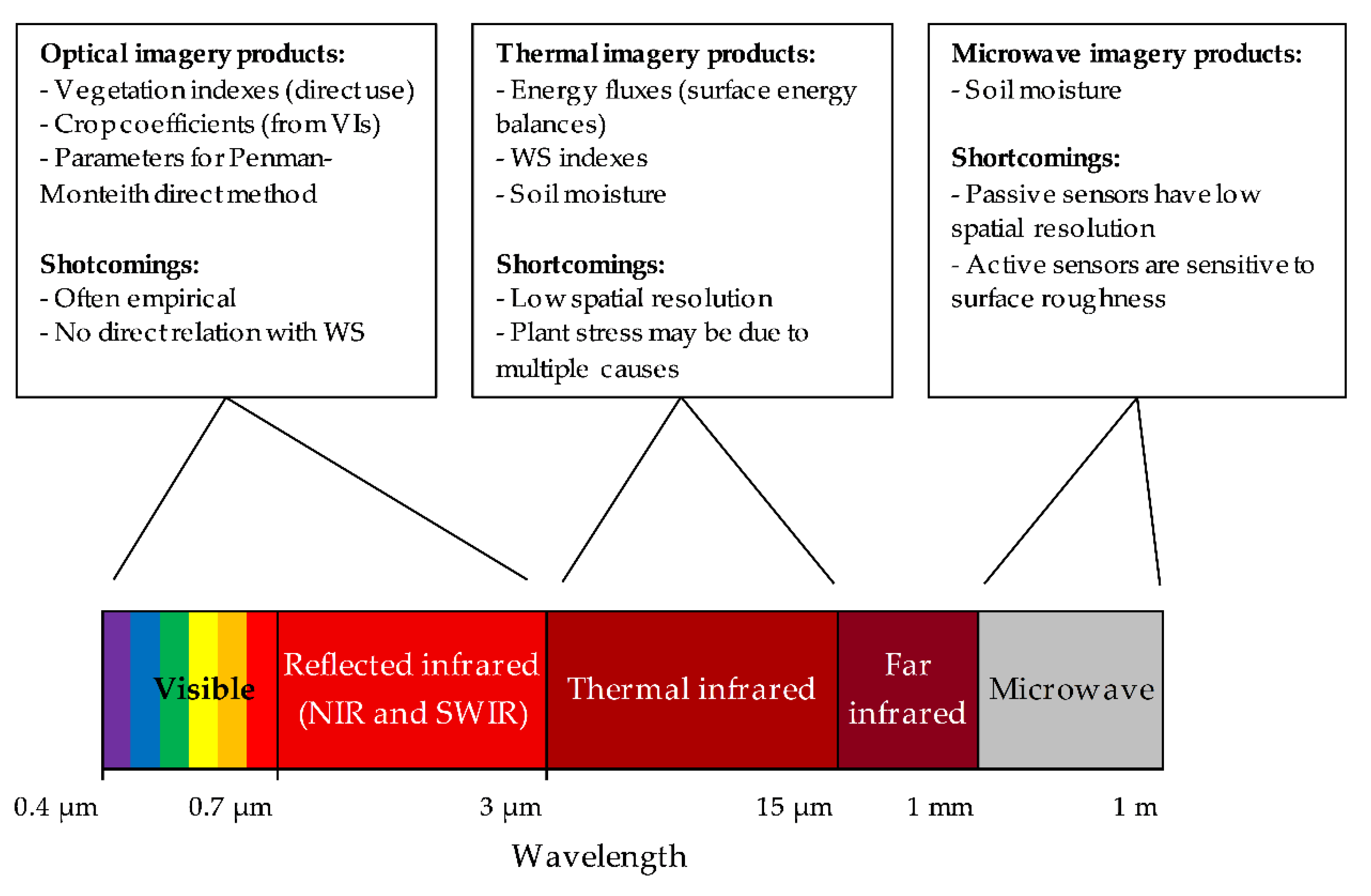
2.1. Radiation Wavelengths for Water Status Estimations

Remote sensing has been used for decades to retrieve information related to crop water stress, at different scales, from global to regional. Concerning field-scale applications, Sishodia et al. [13] recently reviewed the RS methodologies available, e.g., for precision agriculture. The authors identified the main type of information, related to CWR assessment, that can be obtained from RS: (i) crop water stress, (ii) evapotranspiration (ET) and (iii) soil moisture.

In the optical domain, that includes the visible, near infrared (NIR) and shortwave infrared (SWIR) ranges [14], vegetation indices (VIs) are traditionally extracted from RS data to estimate crop biophysical variables. These VIs typically provide precious information on vegetative cover conditions, but detect plant water stress later than indices and relationships calculated from the thermal infrared portion of the spectrum, which are mainly used for the detection of surface (crop and soil) temperature [15]. Optical VIs can eventually be related to the content of plant pigments, that is modified when severe damage has been dealt to the photosynthetic machinery by water stress, whereas thermal imagery provides an earlier pre-visual assessment of water stress, being plant temperature more directly related to transpiration rate [16]. Thermal imagery can be therefore be used to obtain water stress indices, but also to estimate energy fluxes or soil moisture [15]. Methods and indices used to estimate soil moisture which are based on optical and thermal RS have been extensively reviewed by Zhang and Zhou [17], who also mentioned the possibility of using microwave data in this context.

The use of microwave data for field-scale soil moisture estimation is still limited [17]. Passive microwave sensors have a low spatial resolution, while active sensors (e.g., synthetic aperture radar SAR) are sensitive to surface roughness in addition to soil dielectric properties, and only the latter are related to soil moisture [13]. Moreover, SAR data is affected by noise (speckle) that requires spatial or temporal aggregation [18].

Sishodia et al. [13] provide a list and description of the main satellite platforms and VIs used in agriculture, considering not only crop water stress and crop water management, but also other kinds of abiotic and biotic limitations (e.g., nutrient stress or crop diseases). The readers are invited to refer to that paper for further insights, while here we have summarized information and drawbacks of the different RS data types (Figure 1) that are related to their use for the monitoring of plant water stress and water requirements. In fact, VIs, reflectance or thermal parameters and soil moisture are all used in models for the ET estimation or in DSS that share common features with more complex dynamic crop simulation models, thereby suggesting the possibility of integration between them.

The spatial resolution required to obtain relevant crop growth and crop water status estimates needs to be consistent with field-scale management. Sishodia et al. [13], for example, considered satellite platforms whose sensors’ resolution is <30 m as suitable for precision agriculture applications, providing a detailed list. Frequently used and cited satellite platforms are Sentinel 2 for optical data and Landsat family for thermal data. Other satellite platforms that were recurrently used for estimations related to water status were the SPOT constellation (that provides optical data with high spatial resolution, <10–20 m, and high temporal resolution, <10 days), of which SPOT-6 and SPOT-7 are still active, and ASTER (that provides optical and thermal data). MODIS is also often used to downscale soil moisture [19] or surface temperature [20]. Section 2.4 provides examples of the applications of these RS products in this framework.

RS products mentioned above are also used to estimate variables and parameters to be included into two kinds of modeling approaches for the estimation of crop biomass accumulation. These modeling frameworks also constitute the core engine of dynamic crop models, as later discussed in Section 3.1.1 and Section 3.1.2. The water-driven approach estimates crop biomass accumulation as a function of crop evapotranspiration or transpiration. In this context, RS permits to estimate crop coefficients to be used for ET estimations, parameters for direct ET estimations or ET from energy fluxes (see the next Section 2.2). The radiation-driven approach estimates crop biomass accumulation as a function of crop interception/absorption of photosynthetic active radiation. Key variables of this approach, often mentioned in scientific literature, include: the amount of photosynthetic active radiation (PAR), the amount of PAR intercepted by the canopy (IPAR), the amount of PAR absorbed by the canopy (APAR), considered roughly equal to IPAR in most applications, the fraction of absorbed PAR (fAPAR = APAR/PAR) and the fraction of vegetation cover FCOVER (also called fractional canopy cover). In this context, optical RS is mainly used to estimate fAPAR and FCOVER from VIs (as in the examples provided in Section 2.4).

2.2. Modeling Evapotranspiration with Remote Sensing

The FAO (Food and Agricultural Organization) Irrigation and Drainage paper no. 56 [5] has become a standard reference for the estimation of crop water requirements based on evapotranspiration (ET) assessment, which can be easily adapted to RS data [21]. Crop water requirements (CWR) are defined in FAO Irrigation and Drainage paper no. 24 [22] as “the depth of water needed to meet the water loss through evapotranspiration (ETc) of a disease-free crop, growing in large fields under non-restricting soil conditions including soil water and fertility and achieving full production potential under the given growing environment”. In this regard, the FAO-24 paper recommends considering three aspects of the agroecosystem to estimate CWR: (i) the effect of climate on the ET demand, (ii) the effect of crop characteristics on modulating ET and (iii) the effect of local conditions (e.g., soil characteristics) and agricultural practices (e.g., irrigation system) on determining soil water availability.

In this regard, some fundamental concepts and terminologies of the FAO-56 method are necessarily to be briefly recalled here, since they are widely used in RS, DSS and crop modeling communities. The FAO-56 method prescribes the use of the Penman–Monteith equation to estimate reference ET (ET0), with subsequent adjustments to obtain estimates of crop potential ET (ETp) and actual evapotranspiration (ETa). ET0 is the evapotranspiration of a reference hypothetical standard unstressed grass surface. ETp is the evapotranspiration of a specific crop, unstressed, and ETa is the evapotranspiration of a crop under the real field conditions, accounting for WS. Equations (1) and (2) represent the FAO-56 method [5] for calculating potential and actual ET, respectively.

ETp = Kc ∙ ET0    or    ETp = ( Kcb + Ke ) ∙ ET0,

(1)

ETa = Ks ∙ Kc ∙ ET0    or    ETa = ( Ks ∙ Kcb + Ke ) ∙ ET0,

(2)

where the 2 alternatives depend on the method used: the “single coefficient” approach (the first ones) consider the crop field as a whole, while the “dual coefficient” approach (the second ones) separates crop transpiration from soil evaporation. In Equation (1) and (2) Kc is the single crop coefficient (different for each crop and crop stage), similarly to Kcb (the basal crop coefficient); Ke is the soil evaporation coefficient and Ks is the WS coefficient (assuming no other forms of stress are present). The dual coefficient approach is considered more accurate [5].

Calera et al. [7] classify RS-based methods for estimating ET into 3 categories: (i) reflectance-based basal crop coefficients (Kcb), (ii) RS-based Penman–Monteith direct approaches and (iii) RS-based surface energy balance. For a complete description of these methods, we refer readers to the work of Calera et al. [7], of which we provide only a brief but necessary recap. The first two approaches use RS to estimate parameters for ET calculations following the FAO-56 approach.

Reflectance-based Kcb are estimated from VIs and used in the crop dual coefficient approach. The recent review of Pôças et al. [23] on the relationships between crop coefficients and VIs highlighted that, due to the advances of this approach over the last 30 years, such relationships constitute simple and robust operational tools for CWR estimations. Most frequently, these are empirical linear or non-linear relationships between the normalized difference vegetation index (NDVI), the soil adjusted vegetation index (SAVI) and Kc or Kcb. The authors clarified that, due to their empirical nature, these relationships vary with experimental conditions (crop type, irrigation management and climatic conditions), and integration with other approaches (like soil water balance models) are advisable.

RS-based Penman–Monteith direct approaches use RS data to directly estimate the parameters of the Penman–Monteith ETp equation. The rationale behind this approach is that the crop coefficient is a proxy of the parameters describing the canopy development [21,24]. D’Urso and Menenti [24] originally developed the approach by defining analytical functions for the relationships between surface reflectance and vegetation parameters (LAI, surface albedo and crop height) used for the calculation of ETp according to the Penman–Monteith equation. Albedo is used to estimate the net shortwave radiation and LAI and crop height are used in the estimation of canopy resistance. The other weather- and climate-related parameters are derived from air temperature, relative humidity, wind speed and incoming radiation, as usual practice for the Penman–Monteith equation. The equation used in the Penman–Monteith direct method can be expressed as follows (Equation (3) [24,25,26]):

$$\mathrm{ET} = \frac{1}{\mathsf{\lambda }} · \frac{\mathsf{\Delta }\left({\mathrm{R}}_{\mathrm{ns}}{- \mathrm{R}}_{\mathrm{nl}}- \mathrm{G}\right)+{\rho }_a{\mathrm{c}}_{\mathrm{p}}\frac{{(\mathrm{D}}_{\mathrm{E}})}{{\mathrm{r}}_{\mathrm{a}}}}{\mathsf{\Delta } + \mathsf{\gamma }\left(1 + \frac{{\mathrm{r}}_{\mathrm{s}}}{{\mathrm{r}}_{\mathrm{a}}}\right)}$$

(3)

where $\mathsf{\lambda }$, $\mathsf{\Delta }$, ${\mathrm{R}}_{\mathrm{nl}}$, $\mathrm{G}$, ${\rho }_a$, ${\mathrm{c}}_{\mathrm{p}}$, ${\mathrm{D}}_{\mathrm{E}}$ and $\mathsf{\gamma }$ are weather-related variables: $\mathsf{\lambda }$ is the latent heat of vaporization, $\mathsf{\Delta }$ the slope of vapor pressure, ${\mathrm{R}}_{\mathrm{nl}}$ the long-wave net radiation, $\mathrm{G}$ the soil heat flux, ${\rho }_a$ the atmospheric density, ${\mathrm{c}}_{\mathrm{p}}$ the specific heat capacity of air, ${\mathrm{D}}_{\mathrm{E}}$ the vapor pressure deficit and $\mathsf{\gamma }$ the psychrometric constant. ${\mathrm{R}}_{\mathrm{ns}}$, ${\mathrm{r}}_{\mathrm{a}}$, ${\mathrm{r}}_{\mathrm{s}}$, are canopy-related variables derived from RS: ${\mathrm{R}}_{\mathrm{ns}}$ is the shortwave net radiation, ${\mathrm{r}}_{\mathrm{a}}$ the air and ${\mathrm{r}}_{\mathrm{s}}$ the surface resistance. These variables are derived from albedo, LAI and crop height through Equations (4)–(6), respectively:

$${\mathrm{R}}_{\mathrm{ns}} = (1 - \mathsf{\alpha }) ·{ \mathrm{R}}_{\mathrm{ts}}$$

(4)

$${\mathrm{r}}_{\mathrm{s}}=\frac{{\mathrm{r}}_{\mathrm{l}}}{0.5 \mathrm{LAI}}$$

(5)

$${\mathrm{r}}_{\mathrm{a}}=\frac{\ln \left(\frac{{\mathrm{z}}_{\mathrm{u}}-\frac{2}{3}\mathrm{h}}{0.123 \mathrm{h}}\right) · \ln \left(\frac{{\mathrm{z}}_{\mathrm{h}}-\frac{2}{3}\mathrm{h}}{0.0123 \mathrm{h}}\right)}{0.168 \mathrm{U}}$$

(6)

where ${\mathrm{R}}_{\mathrm{ts}}$ is the total incoming shortwave radiation, the surface albedo $\mathsf{\alpha }$ is the spectrally integrated hemispherical solar reflectance, ${\mathrm{r}}_{\mathrm{l}}$ (the average daily value of single leaf resistance) and LAI are used to calculate the surface resistance, while crop height (h), ${\mathrm{z}}_{\mathrm{u}}$ and ${\mathrm{z}}_{\mathrm{h}}$ (measurement height of wind and humidity) and U (wind speed) are used to calculate the aerodynamic resistance. Optical data is used to estimate the required canopy biophysical variables, for example through the use of RS products of the Landsat constellation, SPOT4, ASTER [27] or Sentinel 2 [28].

RS-based surface energy balance (SEB) approaches estimate ET as a residual term of the surface energy balance equation, using thermal data to compute heat fluxes. The concept behind SEBs is that the net energy absorbed by the surface (Rn) should be balanced by the sensible, latent and ground heat fluxes [29]. The balance can also be expressed to explicit the latent heat flux as in Equation (7):

LE = Rn − G − H,

(7)

where LE is the latent heat flux (flux of energy from the Earth’s surface to the atmosphere, that is associated with water evapotranspiration), Rn is the net radiation flux, G the soil heat flux and H the sensible heat flux. Rn consists of the sum of the net shortwave radiation flux (R_ns, determined as in Equation (4)) and the net longwave radiation flux (difference between incident and emitted longwave radiation). Heat fluxes are determined using a wide variety of approaches, that span from empirical direct methods that use locally calibrated constants to simplify the calculations, through methods that merge empirical and mechanistically-based parameterization, up to more deterministic methods [30]. We invite the readers to refer to the review of Courault et al. [30] for a deeper description of the methods used by SEB models to estimate energy fluxes, while some relevant features and differences among SEBs are worth to be mentioned here. A key step of all the SEB models is the estimation of land surface temperature (LST) from thermal imagery for the calculation of the sensible heat flux, while optical imagery in the visible and NIR spectra are used to estimate reflectance-derived canopy characteristics [29]. The loss of sensible heat flux from the surface is determined by aerodynamic temperature, that is usually not directly measured but needs to be derived from RS-obtained radiative temperature [31]. The way this is done defines the main difference between various SEB models, e.g., SEBAL (surface energy balance algorithm for land), TSEB (two source energy balance) and METRIC (mapping evapotranspiration at high resolution with internalized calibration). SEBAL works around the problem of the computation of the relationship between aerodynamic and radiative temperature through the identification of a “wet” and a “dry” pixel in the study area. At the wet surfaces, water vapor is released at a rate that roughly corresponds to 100% of the atmospheric demand, while at dry surfaces the latent heat flux is considered approximately null: this gradient permits the calculation of the sensible heat flux using the spatially-distributed radiometric temperature obtained from RS products [32,33,34]. The TSEB model (two source energy balance) uses a two-source parameterization to account for the contribution of soil and canopy to the heat fluxes and reduce the error of single-source models when applied to sparsely vegetated surfaces [35,36]. METRIC has its foundation on SEBAL, but calibrates internally the model on ground-measured ET0 to reduce the bias in the computation of the energy balance and provide consistency with the traditional methods for ET0 estimations used in agricultural sciences [37].

Overall, Calera et al. [7] provided several examples of successful use of the above-mentioned approaches for ET estimations, but also pointed out their limitations, which are mainly related to: uncertainty in the relationships of reflectance-derived VIs with Kcb or ET equation parameters (for the first two methods), uncertainty in the role of soil evaporation (for the direct ETp approach) and uncertainty in the representativeness of ET estimates over time in the SEB approach, due to the instantaneous nature of RS estimates of ET, corresponding to the timing of satellite overpasses. On the other hand, more accurate estimations of canopy biophysical variables (e.g., albedo, FCOVER and LAI) and more stable relationships with crop coefficients are also more likely to be provided, given the increasing availability of physically-based approaches like radiative transfer models and hybrid methods that combine these models with nonparametric regression and machine learning algorithms [38]. These methods do not present the limits of empirical relationships between VIs and biophysical variables, having a more general validity and being able to make full use of the information stored in the entire radiation spectrum, whereas VIs consider only a few spectral bands.

2.3. Decision Support Systems for Irrigation Scheduling

CWR estimation and irrigation planning can be carried out using decision support systems (DSSs), that simplify features of crop models and integrate them with communication tools to manage inputs and outputs. In practice, a DSS often takes the form of a software that aims at assisting farmers or technicians with decision making on a specific aspect of crop management [39]. To acquire data, DSSs for irrigation scheduling may use either online data (mainly weather data, but also crop and soil data) or data from sensors providing real time information (e.g., from weather stations or soil moisture sensors) [8]. A balance between simplicity and accuracy needs to be struck, since greater accuracy means that more data is required by the model.

DSS come in a great variety of forms and complexity, but usually rely on estimates of ET or soil moisture, using water balance modules. The use of crop and soil simulation modules allow DSSs to provide continuous data on CWR and WS, in order to plan irrigation intervention beforehand and/or adjust irrigation amount based on real-time information. RS data can also be integrated into DSSs to improve predictions. RS permits to collect information on soil moisture, plant growth and plant water status, avoiding at the same time costly and time-consuming field work and the use of more expensive monitoring technologies, with the added benefit of providing spatialized data. This information can be used parameterize the DSS simulation modules or to provide real-time adjustments, in a similar way to more complex crop models (e.g., through data assimilation, discussed in Section 3.5). Recent advances in computer science have also led to the development of DSSs relying on machine learning approaches, that do not need to simulate the behavior of the agroecosystem, but rather find patterns on the collected data (e.g., weather and soil data) and suggest actions to be taken to schedule irrigation [39]. For specific examples of DSSs used in irrigation scheduling, the readers can refer to the recent works of Zhai et al. [39] and Gallardo et al. [8].

Integrating field, proximal sensing and RS data with DSSs has the advantage of providing more accurate and continuous information on crop growth and development, soil water content, CWR and WS. Indeed, Cahn and Johnson [6] pointed out several limitations of measurements, devices and methods used without a comprehensive look at the crop system. Among them we can summarize some that are particularly relevant for this work: (i) soil moisture sensors alone can be useful for determining irrigation timing, but are less useful to determine the irrigation amount, (ii) ET estimates alone may be impractical for scheduling irrigation if not backed up by dynamic assessment of the crop coefficients over time, (iii) soil evaporation calculations require knowledge of soil properties, irrigation methods and interval between irrigation and rainfall events, and (iv) information about the irrigation system (i.e., wetting area, irrigation efficiency, application rate, etc.) needs to be integrated into water requirements calculations.

2.4. Towards Greater Accuracy in Crop Water Stress and Water Requirements Estimations

Some of the approaches mentioned in previous subsections, like RS-based ET estimates or DSS that integrate RS data into simple water balances, have been adjusted and improved over the years to obtain more accurate estimates of WS and CWR. In general, the trend was to increase complexity that could span from the simple addition of CWR indices or thresholds to the integration of entire new modules for better predictions. This tendency can be considered as a logical development aimed at providing an answer to overcome the previously mentioned limitations. Here are some examples:

• The surface energy balance SEBAL was originally conceived to be used with RS imagery at a landscape scale [32,33,34]. Afterwards, throughout the years, several researchers applied SEBAL in the field of agriculture and irrigation, proposing integrations or the use of various stress indices, such as the use of the evaporative fraction (the ratio of latent heat on the sum of latent plus sensible heat [40]) as an indicator of WS that can be considered a substitute of the ETa/ET0 ratio [41], the integration with a crop module for yield estimations [42], the calculation of lumped crop coefficients that incorporate crop and stress coefficients (i.e., Kc multiplied by Ks as in the FAO-56 single coefficient approach) [43], the use of the crop water stress index (CWSI, as in Bhattarai et al. [44]) and the comparison of SEBAL-derived Ks with FAO-56 Ks calculated using soil moisture sensors [45]. However, it is important to stress that SEBAL results are highly sensitive to the choice of the “wet” and “dry” pixels, that are assumed to be representative of fully contrasting hydrological conditions within the area over which the imagery was acquired [46]. Recently, Grosso et al. [47] pointed out that integration of SEBAL with field observations and soil–plant simulations can be particularly beneficial with precision irrigation practices.
• The two-source energy balance TSEB Has undergone subsequent improvements to increase spatial and temporal resolution, for example through data fusion of MODIS and Landsat disaggregated imagery [48]. Recently, Diarra et al. [49] suggested the use of a stress coefficient for monitoring WS with TSEB, based on the ratio between ETa and ETp, following Boulet et al. [50] and using another model for the calculation of the potential conditions. The coefficient ranges between 1 (totally stressed) and 0 (totally unstressed). Similarly, the ratio between actual and potential transpiration has long been used as an indicator of WS also in many crop models, such as DSSAT [51]. Diarra et al. [49] obtained optical imagery (to estimate LAI, vegetation cover and albedo) from SPOT-5 and thermal imagery (to estimate LST) from ASTER.
• FEST-WB (flash flood event based spatially distributed rainfall runoff transformation–water balance) was originally developed as a continuous water balance hydrological distributed model for simulating floods [52]. Later, the model was expanded by integrating energy balance components (FEST-EWB, where the additional E stands for energy) [53], including soil and plant parameters to calculate the water fluxes at the soil surface. The model was built to have a synergic use of RS data. A more recent implementation of FEST-EWB for managing irrigation [54] added crop-specific critical WS thresholds based on soil water content (as in FAO-56 method) to forecast irrigation timing and amount. Vegetation parameters (LAI, FCOVER and albedo) and LST were obtained from Landsat.
• The Italian IRRISAT is a service utilized since 2007 in Campania region (southern Italy), that uses satellite data to provide irrigation prescriptions directly to the farmers (for field level applications) and irrigation districts (for regional applications) [55]. IRRISAT methodology to estimate CWRs is based on the FAO-56 single coefficient direct approach, as detailed by D’Urso [56]. This approach derives crop albedo using weighting coefficient for Sentinel-2 (S2) bands and LAI using artificial neural networks S2 products derived from the Sentinel Application Platform Software (SNAP) biophysical processor. The variables obtained by RS are used as inputs of the Penman–Monteith direct approach for the estimation of ETp. Fixed values for stomatal resistance (100 s m⁻²) and crop height (0.4 m for herbaceous crops) are assumed. Net precipitation is also calculated using the semi-empirical model by Braden [57], that accounts for the effect of canopy interception of rain. A simplified water balance is calculated in this way, and with the help of short-term weather forecasts, CWRs are calculated for each farmer’s field and irrigation district on the interval of 5–7 days. Irrigation prescriptions were originally delivered to the end users in the form of SMS and afterwards through maps and graphs available on more advanced informatic devices (smartphones, tablets etc.). Recently, Bonfante et al. [58] included IRRISAT in LCIS–DSS (low cost irrigation support–DSS). The DSS was built to include 3 different irrigation management tools: (i) W-Tens, a field tensiometer monitoring system with a set of soil water status sensors communicating to a software; (ii) IRRISAT and (iii) W-Mod, based on the SWAP model [59] to simulate crop growth and soil water balance. W-Mod is a physically based simulation model that simulates the vertical flow of water by solving Richards equation (used also in dynamic crop models, see Section 3.2). The equation is solved by applying the hydraulic conductivity relationship proposed by Van Genuchten [60], with the upper boundary condition set by ETp, irrigation and precipitation, with ETp that is partitioned using LAI as suggested by Ritchie [61]. Within W-Mod, the crop growth is simulated by a simple crop module where root growth derived from experimental data on root length and LAI development that follows the “Log Normal Model” of Su et al. [62], that uses maximum LAI and thermal time. Measured data on roots and LAI coming from field trials were used for data assimilation into W-Mod. After field testing, the authors indicated that the integration of W-Tens and IRRISAT can integrate predictions of timing and amount of irrigation, respectively. Integration (via data assimilation in this case) of W-Mod with RS data (instead of field measurements) was also suggested as a potential strategy.
• The Australian IRRISAT is another example of a long lasting DSS service [63,64,65] provided by the Australian research organization CSIRO (Commonwealth and Industrial Research Organization). The DSS uses RS data to estimate reflectance-based crop coefficients from NDVI, using a locally calibrated empirical linear relationships between NDVI and Kc (mainly for cotton, in this case). The Kc (single coefficient) is combined with on-ground ET0 from a net of weather stations to obtain ETc. A simple water balance is calculated using ETc and rainfall and irrigation to provide farmers indication of the amount of water that was used since the last irrigation [63]. Gaynor et al. [66] recently compared the performances of IRRISAT with the HYDROLOGIC crop model on the basis of observed soil moisture, finding greater overall accuracy with IRRISAT, but also better performances of HYDROLOGIC up until peak flowering stages of the crop, despite the limited agronomic information on which HYDROLOGIC was relying. The authors suggested that IRRISAT provided less accurate ET predictions at early stages of canopy growth. This seems to indicate that there is still some room for improving the DSS prediction.
• The SAFY-E (simple algorithm for yield estimation) model [67] was originally created to simulate crop yield with few crop growth and development equations. The availability of the open source Matlab code allows the users to integrate parameters or variables obtained by RS into the model. For example, Duchemin et al. [67] used handheld field measurements of green LAI and NDVI to establish an exponential relationship (potentially useful for RS data too) and calibrate the SAFY model for yield estimation. Subsequent work aimed at including a water balance and WS estimation at the expense of increased complexity. Battude et al. [68] estimated green LAI and FCOVER using high spatial and temporal resolution satellite optical images and integrated a water balance model based on FAO56 method. The satellites used were Formosat-2, SPOT, Landsat-8, Deimos-1 and SPOT4-Take5, all with sufficient spatial resolution for field scale estimates (<30 m). Green, red, NIR and SWIR bands were used for the inversion of the radiative transfer model PROSAIL via artificial neural networks to estimate LAI, FCOVER and fAPAR. LAI was also used as a proxy to estimate Kcb to be used for ET estimations in the FAO-56 method.
• Liu et al. [69] proposed to integrate RS data with a simple radiation-based approach for the calculation of biomass, depending on fAPAR and on RUE (see Section 3.1.2 for definitions and details). The authors used a compact airborne spectrographic imager (CASI) mounted on an airborne platform to obtain hyperspectral RS data during the growing season. In addition, Landsat 5 and Landsat 7 cloud-free images were employed. Surface reflectance from these sensors (visible and NIR range) was combined and used to calculate 2 VIs: NDVI and MTVI2 (modified triangular vegetation index 2). fAPAR was estimated from MTVI2. The canopy structure dynamics model (CSDM) was used to simulate fAPAR dynamics over the season depending on temperature. CSDM was fitted to fAPAR estimated from RS, to derive fAPAR seasonal trend used for the seasonal estimation of biomass accumulation through the radiation driven Monteith approach. In addition, a crop stress index varying between 0 and 1 was added to act as a modifier of the biomass-radiation equation, nullifying the equation when the crop is completely stressed and leaving it unchanged when the crop is unstressed. This approach integrated RS data with simulation of crop cover dynamics, using the radiation-biomass relationship for estimating biomass and yield and a water stress index to limit crop growth, constituting an upgrade of methods based directly on RS data only.
• Campos et al. [70] used VIs obtained from RS data to estimate fAPAR and Kt, a transpiration coefficient similar to Kcb, in order to use these as inputs of simple radiation-driven and water-driven models, respectively (details on the two approaches are provided in Section 3.1). fAPAR and Kt were obtained from relationships with VIs, but the authors contemplated that other analytical approaches could be used to obtain the two biophysical parameters. NDVI obtained by Landsat 5, 7 and 8 were interpolated to obtain daily values to use in the estimation of fAPAR and Kt. Biomass accumulation was then simulated using the radiation-driven and water-driven models.
• Olivera-Guerra et al. [71] developed a method to retrieve irrigation timing and amount at field scale from RS data. Landsat 7 and 8 images with <30% of cloud cover were used over 4 cropping seasons, with an average of 20 images per season. Optical and thermal data from these sensors were used to estimate LST and FCOVER. LST was estimated using the revised single channel algorithm [72], using the thermal band of Landsat, the atmospheric water vapor content from Modis 6.0 and the spectral surface emissivity estimated using the NDVI threshold method proposed by Sobrino et al. [73], that uses FCOVER to weight emissivity from soil and vegetation. Soil emissivity was acquired from ASTER-GED using bands 13 and 14. Vegetation cover was estimated linearly based on minimum and maximum NDVI, following Duchemin et al. [74], and NDVI was obtained from Landsat red and infrared bands. A first guess of root zone soil moisture was obtained for each Landsat overpass date using LST and FCOVER, with a partitioning method based on the LST-FCOVER feature space (e.g., as in Jiang and Islam [75]). The FAO-56 dual coefficient method water balance was applied from the last soil moisture guess, backwards, in a daily time step (recursive mode). The first time that soil moisture reached field capacity (FC) was considered as the day after irrigation was applied, and using the water balance in forward mode from the previous Landsat overpass it was possible to estimate the soil moisture before irrigation started. Since irrigation was assumed to bring soil moisture at FC, irrigation amount could be calculated. In this way, it was possible to reconstruct the soil water and irrigation dynamics (timing and amount) of the entire season of specific fields (by pixel aggregation), providing estimates of water consumption and of crop water requirements when field data are scarce or not available.

In general, in the context of RS and DSS technologies for CWR estimation, WS assessment and irrigation planning, there seems to be a trend on the part of the scientific community to improve these technologies at the cost of added complexity, in order to achieve better characterization of plant–water relationships. In Section 3 we present a categorization of the formalism used by more complex crop models to simulate CWR and WS. This categorization does not aim at providing an exhaustive description of the plant–water relationships of each model, for which we invite the readers to refer to previous studies of Saseendran et al. [76] and Dhakar et al. [77]. It is rather aimed at highlighting common and well-established features that can be useful when improving RS and DSS WS and CWR estimates. Crop models represent a synthesis of the current knowledge about crop processes [78], i.e., an up to date storage of mathematically summarized soil–plant–atmosphere processes that should be considered relevant in the agricultural context. This should also prove useful for the implementation of deficit irrigation, where it is necessary to more precisely quantify also the effects of WS on yield production. As pointed out by Jovanovic et al. [79], deficit irrigation is a complex practice that involves many variables, and optimizing modeling and DSS with holistic approaches are paramount to design the most appropriate strategies for specific crops, varieties and environments, striking a balance between water productivity, environmental safeguard and economic feasibility.

3. Crop Water Stress in Dynamic Crop Models

Complex crop models simulating growth and development of herbaceous and vegetables crops (e.g., maize, wheat, soybean, tomato, etc.) and WS were selected on the basis of the following characteristics. They had to be: (i) freely available, (ii) with an easily accessible documentation, (iii) including water balance and (iv) with options for setting irrigation scheduling rules. The selected models are: APSIM, AQUACROP, CROPSYST, DAISY, DSSAT, EPIC, RZWQM2, STICS. A list of the models, websites and main developer and maintainer is provided in

Table 1. Selected models, website to download software and documentations and core institutions developing and maintaining them.

APSIM	Website	https://www.apsim.info/ [80]
	Main developer	CSIRO, State of Queensland, University of Queensland
AQUACROP	Website	http://www.fao.org/aquacrop/en/ [81]
	Main developer	FAO
CROPSYST	Website	http://modeling.bsyse.wsu.edu/CS_Suite_4/CropSyst/index.html [82]
	Main developer	Washington State University
DAISY	Website	https://daisy.ku.dk/about-daisy/ [83]
	Main developer	University of Copenhagen
DSSAT	Website	https://dssat.net/ [84]
	Main developer	University of Florida
EPIC	Website	https://epicapex.tamu.edu/epic/ [85]
	Main developer	Texas A&M University
RZWQM2	Website	https://data.nal.usda.gov/dataset/rzwqm2 [86]
	Main developer	USDA
STICS	Website	https://www6.paca.inrae.fr/stics_eng/ [87]
	Main developer	INRA

. The formalism of these models will be reviewed in the next subsections by grouping the models according to common features on different aspects of WS and CWR topics. The models will be categorized on the basis of: (i) the functions used to calculate biomass growth and development; (ii) the main variable used to calculate WS coefficients and (iii) the influence of WS on vegetative and reproductive growth. Tracking back the rationale behind crop growth and development can provide opportunities for adjustments of DSSs and RS-related tool used for CWR estimations. As shown in the previous Section 2.4, modeling concepts based on plant processes and soil-water-plant dynamics have often been used to improve existing techniques. Some of these concepts and dynamics are represented in similar ways among different models and different crop modules within the same model. Overall, there is a broad consensus around relevant processes affected by water stress and stress thresholds.

3.1. Water- and Radiation-Driven Crop Growth and Crop Development

A definition of the terms “growth” and “development” is paramount to approach the description of plant-related processes. Following Basso and Ritchie [11], we will consider crop growth as the plant biomass accumulation and crop development as the progression of the plant through growth stages (phenological development). The distinction between these two concepts is of primary importance for the adequate simulation of crop dynamics in different environments.

The selected models can be categorized in “water-driven” and “radiation-driven” models, depending on the mechanism chosen for the simulation of biomass growth.

3.1.1. Water-Driven Models

AQUACROP is a water-driven model developed by FAO. The concepts behind the model are extensively detailed in FAO-66 paper [88], that updates the FAO-33 approach [89] on water productivity and estimates ETa following the FAO-56 method [5]. Model concepts, usage and parameterization are widely described a series of paper from 2009 [90,91,92]. AQUACROP is water-driven, in that the biomass accumulation is directly related to crop transpiration and evapotranspiration, via a crop-dependent water-biomass productivity coefficient (Figure 2). Biomass water productivity has shown a remarkable conservative behavior, remaining nearly constant within species when normalized for the vapor pressure deficit (VPD), as demonstrated in the well-known studies by Tanner and Sinclair [93] and Sinclair et al. [94]. The approach considers that the biomass accumulated by plants in the same environment is directly proportional to the accumulated water volume transpired, being the stomata both the entry point of CO₂ for photosynthesis and the exit point of the absorbed water. The slope of the relationship constitutes the water use efficiency (WUE), i.e., aboveground biomass production per each unit of water transpired. Normalized WUE is considered to be fairly constant for different crops and variates, with major differences between C3 and C4 plants. Figure 2 provides an exemplification of this approach as presented in AQUACROP, where VPD is substituted by ET0 to account for environmental conditions. This modeling concept can give comparable results to that of other more complicated crop models in most situations [95,96], even though some authors questioned its validity under conditions of adequate water supply [97] where agronomic management can play an important role in increasing crop yield, the transpiration efficiency being equal [98]. AQUACROP is still maintained and currently at his 6th version and an open-source Matlab version has recently been released to permit wider use for research purposes by granting access to the source code [99]. This allows easier implementation of inverse modeling techniques and integrating with RS data [100].

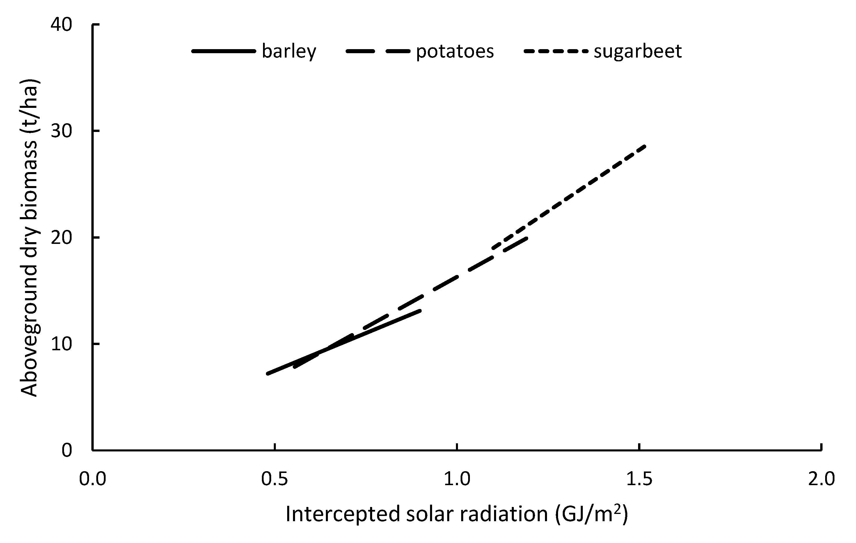
3.1.2. Radiation-Driven Models

DAISY, DSSAT, EPIC, STICS and RZWQM2 are radiation-driven models, i.e., the biomass accumulation is directly (linearly) related to the photosynthetically active radiation (PAR, the radiation between 400 and 700 nm) absorbed or intercepted by canopy (APAR and IPAR, respectively). The slope of this relationship is the radiation use efficiency (RUE, also called light use efficiency, LUE), as detailed in Rosati et al. [101]. The approach used in radiation-driven models is based on early work by Monteith [102,103] (Figure 3). DAISY is described in Abrahamsen and Hansen [104], Hansen [105] and Hansen et al. [106]. The DSSAT (Decision Support System for Agrotechnology Transfer) has been developed and maintained for a long time, currently collecting together two main crop modules: CERES for cereals and CROPGRO, originally for legumes [107,108]. EPIC was initially developed to study the relationship between soil erosion and crop productivity in the US, including simulations of economic related processes [109,110]. STICS is a model with a generic crop module able to adapt to different plants [111,112,113,114]. RZWQM2 (root zone water quality model 2, described in [115]), is an improved version of RZWQM [116] that aims at simulating mainly the fluxes of water, nutrients and chemicals in the root zone, implementing a DSSAT-derived crop module for the simulation of crop growth and development.

3.1.3. Hybrid Models

APSIM [117,118] and CROPSYST [119,120] use a hybrid approach. These models calculate both radiation- and water-driven potential biomass accumulation. Following the law of limiting factors, the lower of the two is kept as the actual biomass accumulation. APSIM 7.1 is the current version to which we will refer, though the research team is working on an improved version called “APSIM Next Gen”. In APSIM, when transpiration is not limiting, soil water demand (transpiration) is calculated backward from the biomass accumulation using the transpiration efficiency normalized by VPD (i.e., using the Tanner–Sinclair relationship in the opposite direction respect to AQUACROP).

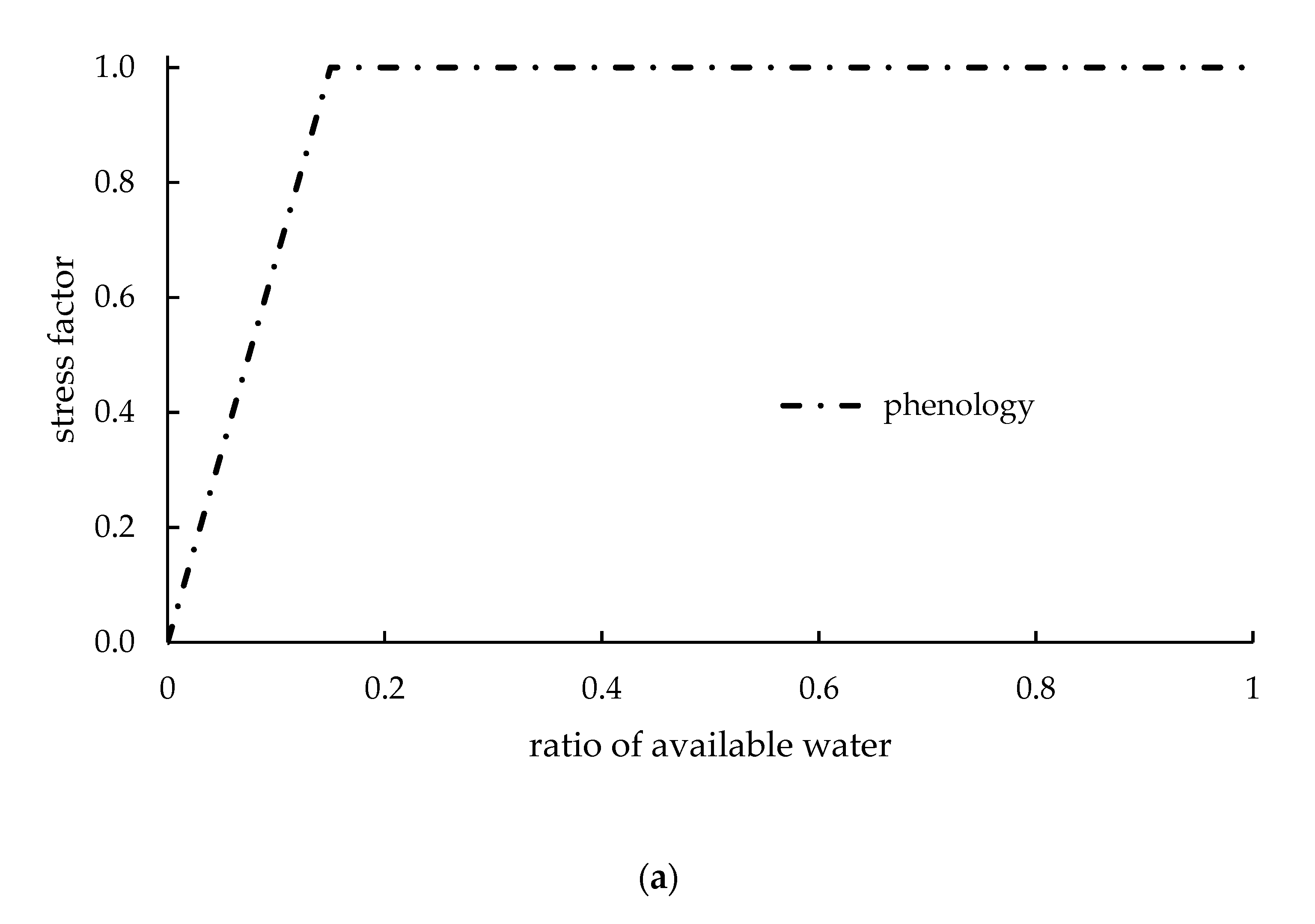
3.1.4. Crop Development

The basic concept used to model crop development is common among all the selected models. Crop development is modeled as a function of thermal time (see the definition in Trudgill et al. [121]), which is expressed in growing degree days (GDD). This is calculated daily, as the difference between the actual temperature and a crop-specific base temperature under which development stops. AQUACROP, for example, simulates crop development using thermal time only, while other models like APSIM include also modifying factors to account for the effects of photoperiod and vernalization. In general, though, further additions to the basic thermal time concept vary between crop modules within the same model (e.g., in DSSAT) and among crop models. The development rate can be accelerated by WS, and WS may have peculiar effects on plant processes in specific growth stages [122], e.g., during flowering and grain filling.

Key state variables that express the canopy development in the selected models are LAI for all the models except AQUACROP. The latter uses the relative canopy cover (called CC in the model, equivalent to the FCOVER of RS), i.e., the percentage of ground surface covered by the canopy, due to its more DSS-oriented nature, since canopy cover is easy to estimate even just by visual estimates or by downward-looking photographs of the crop. This distinction is particularly relevant when the models are integrated with RS since FCOVER is usually easier to estimate than LAI and is not subject to saturation at high values. For example, Silvestro et al. [123] assimilated FCOVER data estimated from HJ1A/B satellite into the AQUACROP model to provide wheat yield estimations at field and district level.

3.2. Soil Water Content and Transpiration Deficit as Inputs of Water Stress Functions

All the selected models can estimate ET0 using the Penman–Monteith formula, except AQUACROP that requires ET0 as an input variable. Within the different models, other less data hungry options are available (e.g., Priestley–Taylor [124]), as well as more complicated ones (e.g., Shuttleworth-Wallace [125]). All the models separate the evaporative fraction of the soil from the transpirative fraction of the plants. The movement of water in soil is simulated either by using solutions of the Richards equation (CROPSYST, DAISY, RZWQM2) or by the simpler cascade approach (AQUACROP, CROPSYST, DSSAT, EPIC, APSIM). The basis of the most frequently used method for separating evaporation and transpiration and for modeling downward flow and root water uptake in a layered soil (cascade approach) are described by Ritchie [51,61]. As for the upward flow (ET-driven), separation of soil evaporation from plant transpiration is dependent on the canopy cover (e.g., through LAI) and is particularly relevant in earlier stages of crop growth, while when the canopy completely covers the ground transpiration contributes the most to the overall ET. As for the downward flow (gravity driven), in the cascade approach excess water (above field capacity) drains to deeper soil layer with a speed that depends on soil hydraulic conductivity.

WS is calculated on the basis of either (i) soil water content or (ii) transpiration deficit.

3.2.1. Soil Water Content

Soil water content for WS calculations is related to the total available water (TAW), where TAW is the difference between field capacity (FC) and plant wilting point (PWP). TAW is also known as plant available water (PAW), root available water or, simply, available water. The input state variable of WS functions can be expressed in relative or absolute values of TAW (e.g., Figure 4 and Figure 5). Other common ways to indicate the soil water limits of TAW are DUL (drain upper limit), that corresponds to field capacity, and LL (lower limit of plant water availability), that corresponds to the wilting point [51]. This alternative nomenclature is common in models derived or inspired by DSSAT. The soil water limits are agronomic concepts used by most crop models to describe in a simplified way relevant soil water potential. However, Ritchie [126,127] warned against the use of water potential to define field water limits to model water balance, especially when the potential is measured with laboratory pressure extraction equipment. The main concerns regard the disturbances related to the extraction of soil cores and the uncertainty around the water potential value of field capacity. These limits should therefore be measured in the field, or through pedotransfer functions [128], that may be already included in the model code and operate automatically.

3.2.2. Transpiration Deficit

Transpiration deficit is expressed as the ratio of potential root water uptake (RWUp) to potential transpiration (Tp), or as a supply/demand ratio (which is the same thing with a different name). Examples are shown in Figure 6 and Figure 7b. RWUp is usually calculated from root density, soil resistance and soil water conductivity [51], and constitutes the potential supply of water from the soil. Tp, obtained by separating the evaporative and transpirative fractions of ETp, represents the potential atmospheric demand of water. When the water supply is greater than the demand (RWUp/Tp > 1), there is no limitation in the transpiration process and the actual transpiration (Ta) is equal to Tp. When the supply is smaller than the demand (RWUp/Tp < 1), the potential water supply is absorbed and transpired completely (RWUp = Ta) and there is a transpirative stress (Ta < Tp).

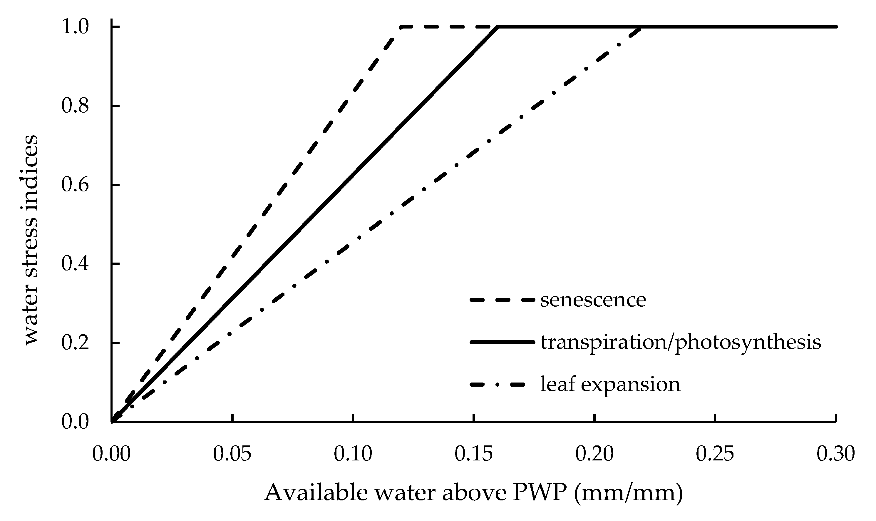
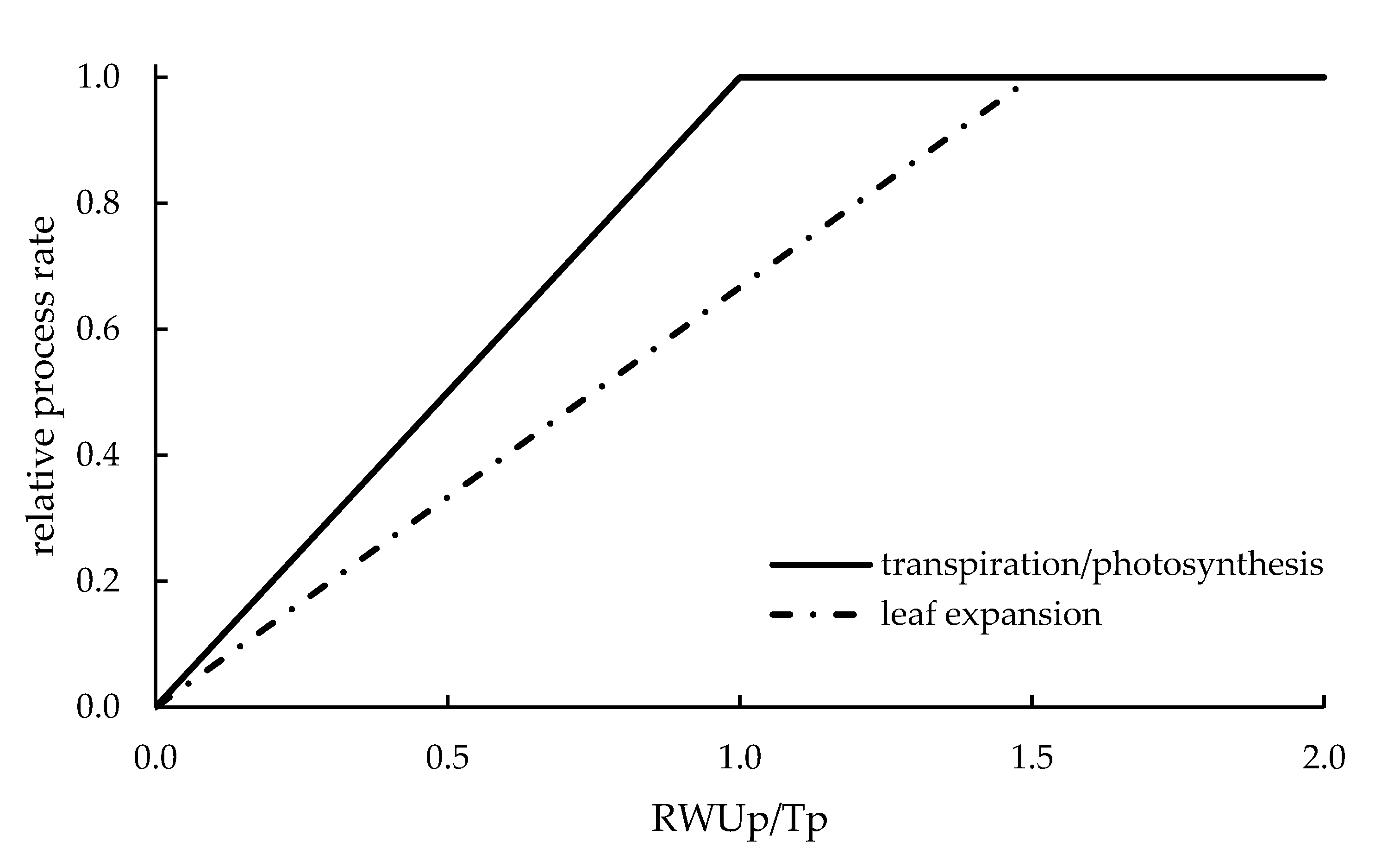
3.2.3. WS Functions Used in Crop Models

To calculate WS functions, AQUACROP uses TAW depletion ratio (Figure 4) and STICS the absolute TAW value (Figure 5). CROPSYST, DAISY, DSSAT, EPIC and RZWQM2 use the transpiration deficit (an example taken from DSSAT is provided in Figure 6). APSIM uses either TAW ratio (Figure 7a) or transpiration deficit (Figure 7b) depending on the process involved. The functions calculate a water stress factor/coefficient/modifier that acts to modify the relative process rate of several target processes. The visual representation of the stress functions of these 4 models covers essentially all the approaches used in the selected models. The processes targeted by WS are discussed in Section 3.3.

3.3. Plant Processes Targeted by Water Stress

For the description of the processes targeted by WS, we will refer from now on to a generic cereal with determinate growth, for simplicity. In particular, for DSSAT we will refer to the DSSAT-CERES crop module and for APSIM to the “Plant” crop module, that replaces previous modules covering the relevant crops. Several functions are used to simulate the WS effects on different plant processes, but the number and type of the effects can differ between crops, especially between determinate and indeterminate crops. Almost all the selected models and crop modules, share similar concepts and formulations of the WS effects on (i) leaf expansion, (ii) transpiration/photosynthesis and (iii) senescence. These functions often come in the models’ documentation or in reference papers with a visual representation of the stress functions on the basis of the state variables used for the calculations (as shown in Section 3.2). Other stress effects are sometimes simulated, but with a lower degree of agreement among different crops and models. These include modifications of the harvest index, acceleration/deceleration of phenology development, shift in photosynthates partitioning to plants’ organs and restrictions to root growth.

Table 2. Summary of the relevant crop models’ features discussed in the paper. R: radiation-driven; W: water driven; R–W: radiation–water hybrid approach (the minimum is kept); LAI: leaf area index; CC: canopy cover (usually called FCOVER in RS); avW: available water (above PWP); Tdef: transpiration deficit (Ta/Tp). Crosses indicate that the model simulates the direct effects of water stress on the specific plant growth or development process.

				Plant Processes Directly Affected by WS:
Model	Biomass Accumulation	Canopy Expansion	WS Function Input Variable	Leaf Expansion	Transpiration-Photosynthesis	Senescence
APSIM (plant module)	R–W	LAI	avW-Tdef	X	X	X
AQUACROP	W	CC (FCOVER)	avW	X	X	X
CROPSYST	R–W	LAI	Tdef	X	X	X
DAISY	R	LAI	Tdef		X
DSSAT (CERES)	R	LAI	Tdef	X	X
EPIC	R	LAI	Tdef	X	X
RZWQM2	R	LAI	Tdef		X
STICS	R	LAI	avW	X	X	X

sums up the relevant information on crop models’ features and processes affected by WS, discussed in detail in the following Sections.

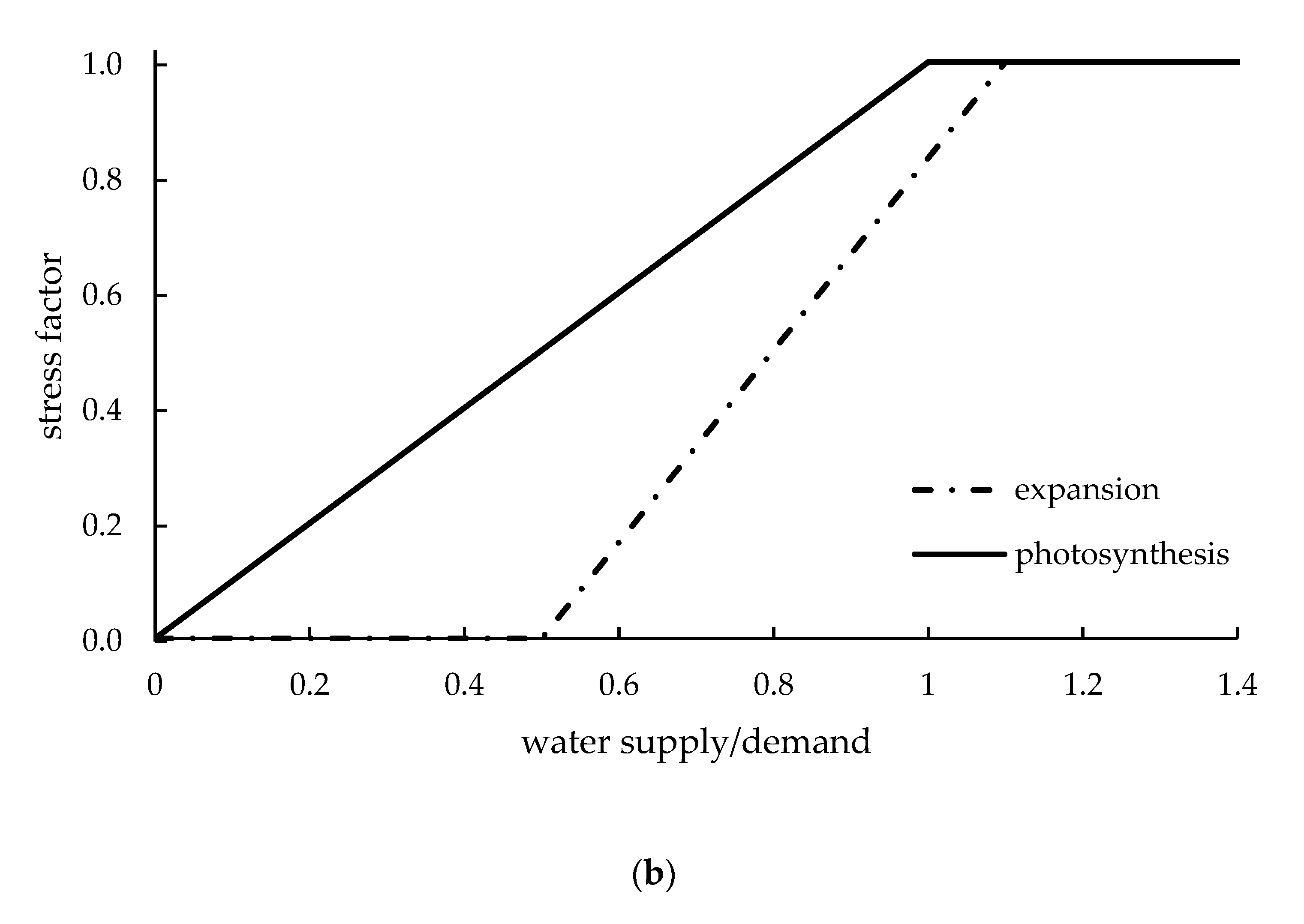
3.3.1. WS Effect on Leaf Expansion

In the progress towards lower soil water content or higher transpiration deficit, the leaf expansion stress is always the first to be encountered, being the most sensitive process. Water stress factors target the equations that regulates canopy/leaf area expansion. From the physiological point of view, WS effect can be thought as a reduction in plant cells turgor and is rarely considered in irrigation planning, especially with RS applications (Section 2). However, some authors pointed out that prolonged mild water stress during the canopy growth period, even if not yet severe enough to inhibit transpiration and photosynthesis, might significantly reduce plant productive capabilities through the steadily reduction of the photosynthetic surface [129,130]. Models that consider this effect of WS are: APSIM (Figure 7b), AQUACROP (Figure 4), CROPSYST (where leaf expansion completely stops when the Ta/Tp ratio drops below 0.9), DSSAT (Figure 6), EPIC (where the WS can reduce LAI expansion) and STICS (Figure 5). In all these cases leaf expansion is considered the process most sensitive to WS. DAISY and RZWQM2 do not simulate direct effect of WS on leaf expansion.

3.3.2. WS Effect on Transpiration/Photosynthesis

The WS effect on stomatal conductance affects biomass accumulation through reduced transpiration or reduced photosynthesis (due to reduced transpiration), depending on the formulation of each model. From the physiological point of view, water deficit causes stomata closure, reducing transpiration and CO₂ assimilation and, in turn, photosynthesis and biomass accumulation. Irrigation scheduling usually aims at avoiding completely stomatal closure (except for deficit irrigation), as highlighted by Jovanovic et al. [79]. This stress is so important and limiting that it is simulated by all the selected models. APSIM (Figure 7b), CROPSYST, DAISY, DSSAT (Figure 6), EPIC and RZWQM2 use the Ta/Tp ratio to reduce the biomass accumulation (in RZWQM2 the relationship between WS coefficient and transpiration deficit is nonlinear [131]. In DAISY, the biomass reduction is the only effect of WS considered. The reduction is based on soil water content in AQUACROP (Figure 4) and STICS (Figure 5), where the stress coefficient reduces transpiration and photosynthesis, respectively.

3.3.3. WS Effect on Senescence

WS can increase the senescence rate and also cause an earlier onset of senescence. The senescence process is affected by WS in most of the models and is the least sensitive process in respect to leaf expansion and transpiration reduction (see Figure 4 and Figure 5). Senescence is affected either through a direct increase in senescence rate or through a decrease in leaf area duration (LAD) and adjustment of the LAI curve. WS effect on senescence is modeled in APSIM, using WS factor for photosynthesis (Figure 7b), AQUACROP (Figure 4), CROPSYST, where senescence is determined by LAD and STICS (Figure 5). DAISY, DSSAT-CERES, EPIC and RZWQM2 do not directly model this effect.

3.3.4. WS Effect on Other Processes

WS can also influence harvest index (HI), phenology, partitioning and root growth, but these effects are not modeled consistently in all the models. HI is modified by WS in APSIM, AQUACROP, CROPSYST and EPIC, mainly during flowering and grain filling period. In APSIM, WS reduces HI depending on stress severity and a sensitivity factor. AQUACROP derives a HI modifier from the stress coefficients of leaf expansion (that increases HI) and of transpiration (that instead decreases HI). CROPSYST reduces HI using the lowest of water and N stress, with different sensitivity depending on stage. In EPIC, WS acts on HI depending on the stress range: with low WS (coefficient > 0.9) the HI increases, with higher WS (coefficient between 0.3 and 0.9) the HI decrease [110]. In general, it is suggested that moderate stress can be beneficial (increase in HI, in some models), while more severe WS is always detrimental for production (decrease in HI).

WS effect on development (phenology) is modeled in APSIM (Figure 7a), CROPSYST, STICS and RZWQM2. Development is slowed down by WS in APSIM from emergence to flowering, while in CROPSYST and STICS it is hastened (due to an increase in crop temperature, that governs development) [113]. In RZWQM2 moderate WS (Ta/Tp > 0.6) can hasten development, while severe stress (Ta/Tp < 0.6) slows it down.

A shift in partitioning can also be caused by WS in some of those models that simulate photosynthates allocation in different parts of the plant, but there is no consistent way of simulating it among the models. DSSAT-CERES shift allocation towards roots during WS, APSIM towards grain during grain filling period if there are not enough photosynthates, EPIC simulates root growth on the basis of RWU, RZWQM2 reduces partitioning to shoots under WS. Root growth can also be restricted by low soil water content, as in APSIM, DSSAT and STICS.

3.4. Comparison of Dynamic Crop Models

To choose the most suitable approach to model crop growth, CWR and WS is up to the modeler, depending on the purpose of the research or application, the desirable level of model complexity, data availability and user friendliness. The question of which model is “the best” has, therefore, virtually no univocal answer. Choosing a more complex and detailed model is not always a guarantee of getting better results than using a simpler, well calibrated model. However, research experience accumulated in scientific literature, comparing the performances of different models to field data in the presence of water limitations, can help to understand specific features of each model. For this reason, a few examples of model comparison will be discussed. Only the models previously discussed and reported in Table 2 will be considered.

Kloss et al. [132] compared among others DAISY and APSIM performances in simulating crop growth under deficit irrigation using field data from India, Malawi, France and Oman. The authors noticed that the yield reduction simulated by DAISY in cases of severe water stress was smaller and further from reality than for APSIM. The authors suggested that in the cases of severe water stress, especially when after a stress period full irrigation was restored, DAISY was unable to simulate irreversible damage to the crop. Even if photosynthesis was reduced during drought stress, when water availability was fully restored, both potential transpiration and photosynthesis where reached again at the same levels than before. On the other hand, APSIM also models WS effects on leaf expansion, phenology and partitioning, as previously shown in Section 3.3. However, the authors also stressed that the severe and alternating stress conditions where DAISY simulation fell short are unlikely to be met in non-experimental conditions.

Todorovic et al. [95] compared AQUACROP and CROPSYST performances in simulating sunflower growth under deficit irrigation over two cropping seasons in Southern Italy, i.e., in a Mediterranean climate. The experimental treatments were designed to provide deficit irrigation during the whole season, but also to differentiate it before and after flowering. AQUACROP performed similarly to CROPSYST, but required fewer inputs. CROPSYST simulated better the WUE under severe water stress. The authors suggested that the physiological submodel that simulates crop growth and partitioning in AQUACROP is more simplified than in CROPSYST, thus justifying the lower performances under severe water stress. Indeed, as explained in Section 3.3, CROPSYST simulates WS effect on phenology (hastening development under WS), while AQUACROP does not, and the effect on HI is also more detailed. However, the authors stressed that both models performed well under moderate stress conditions, and that their results might have been influenced by the manual calibration and the short duration of the experiment, suggesting that automatic calibration over multiple years may produce better results.

Abi Saab et al. [96] also compared AQUACROP and CROPSYST. The field experiment was on barley cultivated over 3 years, with treatments including rainfed conditions, full irrigation (maintaining full transpiration) and 50% of full irrigation. The calibration year was alternated to check the effect of calibration on the performance of the models on the validation datasets. In general, AQUACROP showed better performances, but the model was recalibrated for each non-optimal N supply conditions, while CROPSYST was calibrated once for each year (under optimal N supply conditions). This was due to the lack of a N balance module in AQUACROP. The authors suggested that CROPSYST should be a better choice in when nutrient and water stress are balanced, while when the yield reduction is due to water stress alone, AQUACROP may be preferable.

Rötter et al. [133] tested several models over 14 years of data for spring barley over multiple locations and various weather conditions. Among the models, CROPSYST, DAISY, DSSAT-CERES and STICS were included. The models were given to groups of users, to perform a “blind test”: limited data was available for calibration (only phenological observations) and the modelers were allowed to calibrate only phenological parameters. Overall, yield estimates were unsatisfactory, with measurement error > 10–15 % respect to the observed yield. The uncertainty in the estimation was similar to that found by Palosuo et al. [134] for wheat, even though the initial hypothesis of the authors was that the uncertainty was higher since barley had been less studied by the modeling community, thus having more imprecise formalism and parameters. The authors proposed that one of the reasons for the lower-than-expected error of barley simulations could have been the shorter cycle of spring barley and the absence of vernalization processes to be simulated, that instead were thought to have played a relevant role in increasing the uncertainty of winter wheat predictions in Palosuo et al. [134]. Overall, the phenology showed considerable discrepancies between simulated and observed data. The authors suggested that the complexity of effects of water and nutrient limitation in delaying or hastening the phenological development was probably not caught in sufficient detail by all the selected models. At the same time, though, the models with more accurate estimations of phenology, they did not necessarily predict yield more accurately. As for grain yield, DAISY and CROPSYST systematically underestimated yield, while the greatest variance in model residuals (inaccuracy of the estimation) was found in DSSAT-CERES, while DAISY showed the strongest correlation between observed and simulated yield (lowest uncertainty).

Kimball et al. [135] compared ET estimates among 29 models or model versions given to several modelers’ groups to simulate 8 years of maize monocropping in Iowa. Among the models, CROPSYST, RZWQM2, and various versions of APSIM, DSSAT-CERES and STICS were used. Differences between versions regarded mainly the ET estimation process (e.g., using different equations). The study was conducted in 4 phases: (i) a “blind phase” where only key input data on soil, weather and management and anthesis and maturity dates were provided; (ii) a “LAI phase” where LAI observations time series were provided, to see if improving simulations of leaf expansion also improved ET predictions; (iii) a phase where also observations of biomass, yield, ET and soil moisture of a typical year for rainfall was provided and (iv) a phase where all the observations were provided for all years to allow for detailed calibration. Overall, supplying LAI for all the years led only to slight improvements of ET estimates. With the additional information of phase 4, APSIM versions that used the Priestley–Taylor approach to estimate ET were the models that provided better evaporation estimates during early phases of crop growth. This highlighted the importance of providing information on crop variables to improve ET estimations and of providing good early-stage predictions of soil evaporation and leaf area development to obtain accurate measurements of seasonal ET. ETa during mid-season (when Ta contributes to a greater extent) was usually better predicted through the FAO-56 Penman–Monteith approach or the Shuttleworth-Wallace approach (RZWQM2 and a version of STICS). The authors noted little overlap among the models identified as best for the early-stage, evaporation-dominated period and for the mid-season, T-dominated period, suggesting that models should be improved by combining the best approaches to simulate evaporation with those to simulate T. Considering the performances on estimating both ET and agronomic variables (LAI, biomass and yield) after full calibration (phase 4), the median of all the models ranked first, followed by versions of APSIM and DSSAT-CERES (among the models selected for this review).

3.5. Integration of RS Data and Crop Models

DSS platforms to support irrigation scheduling often already include simple statistical or mechanistic models. In this framework, the application to DSSs of the concepts highlighted for dynamic models consists of a revision of the formalism of the DSS, or the addition of further simulation modules, e.g., water balance module or crop growth and development module, when this is considered appropriate. On the other hand, RS imagery requires subsequent elaborations to be used to estimate crop growth and development, WS and CWR, ranging between different degrees of complexity and directness. From the operational point of view, one of the most complicated and indirect, yet promising procedure, is the integration of RS data with dynamic crop models. RS data can be considered a natural partner of crop models, as testified by historical developments highlighted by Pinter et al. [136] and Jones et al. [9]. Kasamplis et al. [137] stressed that one of the major limitations of crop models at field scale is the lack of spatial information of the conditions within the fields, but RS can provide this information to improve models’ predictions. RS can be used to estimate state variables of crop models like FCOVER, LAI and fAPAR. One of the methods for integrating RS data with crop models that has received increased attention is data assimilation [138]. Three different strategies can be used to integrate biophysical variables derived from RS observations into crop models: calibration, forcing and updating [139]. As a rule of thumb, calibration adjusts the model parameters to minimize differences between historical observed and simulated data without considering the uncertainty contained in the observed data, forcing methods replace simulated with observed data having the same time-step (daily in most crop models) and the updating methods usually provide a real-time adjustment of model parameters considering the uncertainty related to both simulated and observed data [139].

Crop models integrating RS data can be used to provide a continuous characterization of the agroecosystem over time and forecasts of its future state, which is something that RS alone struggles to do [138]. In addition, modeling approaches permit to separate crop stresses and processes, while RS measures the actual growth conditions that includes the combined effects of growth reduction factors (e.g., water and nutrient stress together) [140]. Data assimilation can also integrate simultaneously several types of data into the same modeling scheme, e.g., multisource RS data, as well as data from airborne, Unmanned Aerial Vehicles (UAVs) and ground proximal sensors platforms. It also allows the use of near real-time meteorological data and forecasts.

In this context, users can select models based on their needs and on the best approach that fits available data from RS or other sources. The modeled effects of WS on specific plant processes of interest can also be considered. For example, correct quantification of water stress effects on crop biomass and yield are paramount in cases of deficit irrigation, where the assessment of a stress/unstressed condition is not enough to maximize the efficiency of the irrigation water use, rather than maximizing yield. Or else, a representation of water stress effects on leaf expansion might be useful in environments characterized by prolonged moderate stress during early stages of crop growth. Equations and approaches from crop models presented in this work can provide examples to implement further RS and DSS-based estimations of WS and CWR. At the same time, an overview that can guide the users through the choice of the model best suited for their purposes is provided.

4. Conclusions

We have provided an overview of recent approaches based on remote sensing and decision support systems conceived for aiding in the management of crop water requirements and water stress, highlighting relevant steps undertaken over the years to improve these tools. A general trend of increasing complexity can be noticed, with the aim of introducing relevant features or adjustment to better fulfill irrigation management support. ET estimation from remote sensing imagery and advices from decision support systems offer great opportunities for scheduling irrigation, but are limited by an incomplete representation of the soil–plant–atmosphere dynamics. Dynamic crop models offer a better understanding of the processes related to water stress, but are usually more suitable for research purposes than for direct applications by farmers and agricultural technicians. However, freely available dynamic crop models with accessible documentation (such as APSIM, AQUACROP, CROPSYST, DAISY, DSSAT, EPIC, RZWQM2 and STICS) stand as a source of condensed knowledge on the processes governing plant water stress and stress effects on plant growth and development. To some degree, these models share concepts and formalism that can be classified together. The models simulate biomass accumulation from crop transpiration, intercepted radiation or using both the approaches and selecting the most limiting. Stress functions are based on soil water content or deficit transpiration. The main processes affected by water stress in similar ways among the models include: leaf expansion (the most sensitive), transpiration/photosynthesis (usually determining irrigation thresholds, since it heavily affects biomass accumulation) and senescence. The information provided, along with the references to relevant documents and papers regarding these concepts, may constitute a starting point for researchers seeking to improve RS and DSS approaches in the field of water stress and crop water requirements estimations. The best of these worlds can be combined and integrated in several ways, keeping in mind that the choice to be made should comply with the final goal to be pursued. Who is the end user? Which degree of operational complexity should be allowed? What is the temporal perspective of interest: predictions, real-time information, or both? Is a qualitative indication of water status enough, or is a quantification of water stress effects on plant processes more appropriate? Does irrigation timing and amount need to be accurately assessed? All are questions worth asking when choosing the most appropriate approach.

References

1. Huang, Z.; Hejazi, M.; Tang, Q.; Vernon, C.R.; Liu, Y.; Chen, M.; Calvin, K. Global agricultural green and blue water consumption under future climate and land use changes. J. Hydrol. 2019, 574, 242–256. [Google Scholar] [CrossRef]
2. Mekonnen, M.M.; Hoekstra, A.Y. Sustainability of the blue water footprint of crops. Adv. Water Resour. 2020, 143, 103679. [Google Scholar] [CrossRef]
3. UNESCO World Water Assessment Programme. United Nations World Water Development Report 2020: Water and Climate Change; UNESCO: Paris, France, 2020; ISBN 978-92-3-100371-4. [Google Scholar]
4. More Crop per Drop: Revisiting a Research Paradigm: Results and Synthesis of IWMI’s Research, 1996–2005; Giordano, M.; Rijsberman, F.R.; Saleth, R.M. (Eds.) IWA Publishing: London, UK, 2007. [Google Scholar] [CrossRef]
5. Allen, R.G.; Pereira, L.S.; Raes, D.; Smith, M. Crop Evapotranspiration: Guidelines for Computing Crop Water Requirements; FAO Irrigation and Drainage Paper 56; FAO: Rome, Italy, 1998; ISBN 92-5-104219-5. [Google Scholar]
6. Cahn, M.D.; Johnson, L.F. New approaches to irrigation scheduling of vegetables. Horticulturae 2017, 3, 28. [Google Scholar] [CrossRef] [Green Version]
7. Calera, A.; Campos, I.; Osann, A.; D’Urso, G.; Menenti, M. Remote sensing for crop water management: From ET modelling to services for the end users. Sensors 2017, 17, 1104. [Google Scholar] [CrossRef] [PubMed] [Green Version]
8. Gallardo, M.; Elia, A.; Thompson, R.B. Decision support systems and models for aiding irrigation and nutrient management of vegetable crops. Agric. Water Manag. 2020, 240, 106209. [Google Scholar] [CrossRef]
9. Jones, J.W.; Antle, J.M.; Basso, B.; Boote, K.J.; Conant, R.T.; Foster, I.; Godfray, H.C.J.; Herrero, M.; Howitt, R.E.; Janssen, S.; et al. Brief history of agricultural systems modeling. Agric. Syst. 2017, 155, 240–254. [Google Scholar] [CrossRef]
10. Delécolle, R.; Maas, S.J.; Guerif, M.; Baret, F. Remote sensing and crop production models: Present trends. ISPRS J. Photogramm. Remote Sens. 1992, 47, 145–161. [Google Scholar] [CrossRef]
11. Basso, B.; Ritchie, J.T. Simulating crop growth and biogeochemical fluxes in response to land management using the SALUS model. In The Ecology of Agricultural Landscapes: Long-Term Research on the Path to Sustainability; Hamilton, S.K., Doll, J.E., Robertson, G.P., Eds.; Oxford University Press: New York, NY, USA, 2015; pp. 252–274. ISBN 9780199773350. [Google Scholar]
12. Weiss, M.; Jacob, F.; Duveiller, G. Remote sensing for agricultural applications: A meta-review. Remote Sens. Environ. 2020, 236, 111402. [Google Scholar] [CrossRef]
13. Sishodia, R.P.; Ray, R.L.; Singh, S.K. Applications of remote sensing in precision agriculture: A review. Remote Sens. 2020, 12, 3136. [Google Scholar] [CrossRef]
14. Prasad, S.; Bruce, L.M.; Chanussot, J. (Eds.) Optical remote sensing—Advances in Signal Processing and Exploitation Techniques; Springer: Berlin/Heidelberg, Germany, 2011. [Google Scholar] [CrossRef]
15. Khanal, S.; Fulton, J.; Shearer, S. An overview of current and potential applications of thermal remote sensing in precision agriculture. Comput. Electron. Agric. 2017, 139, 22–32. [Google Scholar] [CrossRef]
16. Gerhards, M.; Schlerf, M.; Mallick, K.; Udelhoven, T. Challenges and future perspectives of multi-/Hyperspectral thermal infrared remote sensing for crop water-stress detection: A review. Remote Sens. 2019, 11, 1240. [Google Scholar] [CrossRef] [Green Version]
17. Zhang, D.; Zhou, G. Estimation of soil moisture from optical and thermal remote sensing: A review. Sensors 2016, 16, 1308. [Google Scholar] [CrossRef] [PubMed] [Green Version]
18. Tupin, F.; Denis, L.; Deledalle, C.A.; Ferraioli, G. Ten Years of Patch-Based Approaches for Sar Imaging: A Review. In Proceedings of the IEEE International Geoscience and Remote Sensing Symposium, Yokohama, Japan, 28 July–2 August 2019. [Google Scholar] [CrossRef] [Green Version]
19. Im, J.; Park, S.; Rhee, J.; Baik, J.; Choi, M. Downscaling of AMSR-E soil moisture with MODIS products using machine learning approaches. Environ. Earth Sci. 2016, 75, 1120. [Google Scholar] [CrossRef]
20. Duan, S.B.; Li, Z.L. Spatial downscaling of MODIS land surface temperatures using geographically weighted regression: Case study in northern China. IEEE Trans. Geosci. Remote Sens. 2016, 54, 6458–6469. [Google Scholar] [CrossRef]
21. Vuolo, F.; D’Urso, G.; De Michele, C.; Bianchi, B.; Cutting, M. Satellite-based irrigation advisory services: A common tool for different experiences from Europe to Australia. Agric. Water Manag. 2015, 147, 82–95. [Google Scholar] [CrossRef]
22. Doorenbos, J.; Pruitt, W.O. Crop Water Requirements; FAO Irrigation and Drainage Paper No. 24; FAO: Rome, Italy, 1977. [Google Scholar]
23. Pôças, I.; Calera, A.; Campos, I.; Cunha, M. Remote sensing for estimating and mapping single and basal crop coefficientes: A review on spectral vegetation indices approaches. Agric. Water Manag. 2020, 233, 106081. [Google Scholar] [CrossRef]
24. D’Urso, G.; Menenti, M. Mapping crop coefficients in irrigated areas from Landsat TM images. Proc. SPIE 1995, 2585, 41–47. [Google Scholar] [CrossRef]
25. D’Urso, G.; Menenti, M.; Santini, A. Regional application of one-dimensional water flow models for irrigation management. Agric. Water Manag. 1999, 40, 291–302. [Google Scholar] [CrossRef]
26. Pasqualotto, N.; D’Urso, G.; Bolognesi, S.F.; Belfiore, O.R.; Van Wittenberghe, S.; Delegido, J.; Pezzola, A.; Winschel, C.; Moreno, J. Retrieval of evapotranspiration from Sentinel-2: Comparison of vegetation indices, semi-empirical models and SNAP biophysical processor approach. Agronomy 2019, 9, 663. [Google Scholar] [CrossRef] [Green Version]
27. D’Urso, G.; Calera, A. Operative approaches to determine crop water requirements from Earth Observation data: Methodologies and applications. AIP Conf. Proc. 2006, 852, 14. [Google Scholar] [CrossRef]
28. Vanino, S.; Nino, P.; De Michele, C.; Bolognesi, S.F.; D’Urso, G.; Di Bene, C.; Pennelli, B.; Vuolo, F.; Farina, R.; Pulighe, G.; et al. Capability of Sentinel-2 data for estimating maximum evapotranspiration and irrigation requirements for tomato crop in Central Italy. Remote Sens. Environ. 2018, 215, 452–470. [Google Scholar] [CrossRef]
29. Hall, F.G.; Huemmrich, K.F.; Goetz, S.J.; Sellers, P.J.; Nickeson, J.E. Satellite remote sensing of surface energy balance: Success, failures, and unresolved issues in FIFE. J. Geophys. Res. Atmos. 1992, 97, 19061–19089. [Google Scholar] [CrossRef]
30. Courault, D.; Seguin, B.; Olioso, A. Review on estimation of evapotranspiration from remote sensing data: From empirical to numerical modeling approaches. Irrig. Drain. Syst. 2005, 19, 223–249. [Google Scholar] [CrossRef]
31. Chehbouni, A.; Seen, D.L.; Njoku, E.G.; Monteny, B.M. Examination of the difference between radiative and aerodynamic surface temperatures over sparsely vegetated surfaces. Remote Sens. Environ. 1996, 58, 177–186. [Google Scholar] [CrossRef]
32. Bastiaanssen, W.G.M. Regionalization of Surface Flux Densities and Moisture Indicators in Composite Terrain: A Remote Sensing Approach under Clear Skies in Mediterranean Climates. Ph.D. Thesis, Wageningen University, Wageningen, The Netherlands, 1995. ISBN 90-5485-465-0. [Google Scholar]
33. Bastiaanssen, W.G.M.; Menenti, M.; Feddes, R.A.; Holtslag, A.A.M. A remote sensing surface energy balance algorithm for land (SEBAL). 1. Formulation. J. Hydrol. 1998, 212, 198–212. [Google Scholar] [CrossRef]
34. Bastiaanssen, W.G.M.; Pelgrum, H.; Wang, J.; Ma, Y.; Moreno, J.F.; Roerink, G.J.; Van der Wal, T. A remote sensing surface energy balance algorithm for land (SEBAL): Part 2: Validation. J. Hydrol. 1998, 212, 213–229. [Google Scholar] [CrossRef]
35. Norman, J.M.; Kustas, W.P.; Humes, K.S. Source approach for estimating soil and vegetation energy fluxes in observations of directional radiometric surface temperature. Agric. For. Meteorol. 1995, 77, 263–293. [Google Scholar] [CrossRef]
36. Kustas, W.P.; Norman, J.M. Evaluation of soil and vegetation heat flux predictions using a simple two-source model with radiometric temperatures for partial canopy cover. Agric. For. Meteorol. 1999, 94, 13–29. [Google Scholar] [CrossRef]
37. Allen, R.G.; Tasumi, M.; Trezza, R. Satellite-based energy balance for mapping evapotranspiration with internalized calibration (METRIC)—Model. J. Irrig. Drain. Eng. 2007, 133, 380–394. [Google Scholar] [CrossRef]
38. Upreti, D.; Huang, W.; Kong, W.; Pascucci, S.; Pignatti, S.; Zhou, X.; Ye, H.; Casa, R. A comparison of hybrid machine learning algorithms for the retrieval of wheat biophysical variables from Sentinel-2. Remote Sens. 2019, 11, 481. [Google Scholar] [CrossRef] [Green Version]
39. Zhai, Z.; Martínez, J.F.; Beltran, V.; Martínez, N.L. Decision support systems for agriculture 4.0: Survey and challenges. Comput. Electron. Agric. 2020, 170, 105256. [Google Scholar] [CrossRef]
40. Shuttleworth, W.J.; Gurney, R.J.; Hsu, A.Y.; Ormsby, J.P. FIFE, the variation on energy partition at surface flux sites. In Proceedings of the International Association of Hydrological Sciences (IAHS) Third Scientific Assembly, Baltimore, MD, USA, 10–19 May 1989; pp. 67–74. [Google Scholar]
41. Bastiaanssen, W.G.M. SEBAL-based sensible and latent heat fluxes in the irrigated Gediz Basin, Turkey. J. Hydrol. 2000, 229, 87–100. [Google Scholar] [CrossRef]
42. Bastiaanssen, W.G.M.; Ali, S. A new crop yield forecasting model based on satellite measurements applied across the Indus Basin, Pakistan. Agric. Ecosyst. Environ. 2003, 94, 321–340. [Google Scholar] [CrossRef]
43. Lal, D.; Clark, B.; Bettner, T.; Thoreson, B.; Snyder, R. Rice evapotranspiration estimates and crop coefficients in Glenn-Colusa irrigation district, Sacramento Valley, California. In Irrigated Agriculture Responds to Water Use Challenges—Strategies for Success, Proceedings of the USCID Water Management Conference, Austin, TX, USA, 3–6 April 2012; Gibbens, G.A., Anderson, S.S., Eds.; U.S. Committee on Irrigation and Drainage: Denver, CO, USA; pp. 145–156. ISBN 978-1-887903-39-4.
44. Bhattarai, N.; Wagle, P.; Gowda, P.H.; Kakani, V.G. Utility of remote sensing-based surface energy balance models to track water stress in rain-fed switchgrass under dry and wet conditions. ISPRS J. Photogramm. Remote Sens. 2017, 133, 128–141. [Google Scholar] [CrossRef]
45. Gobbo, S.; Lo Presti, S.; Martello, M.; Panunzi, L.; Berti, A.; Morari, F. Integrating SEBAL with in-Field Crop Water Status Measurement for Precision Irrigation Applications—A Case Study. Remote Sens. 2019, 11, 2069. [Google Scholar] [CrossRef] [Green Version]
46. Timmermans, W.J.; Kustas, W.P.; Anderson, M.C.; French, A.N. An intercomparison of the surface energy balance algorithm for land (SEBAL) and the two-source energy balance (TSEB) modeling schemes. Remote Sens. Environ. 2007, 108, 369–384. [Google Scholar] [CrossRef]
47. Grosso, C.; Manoli, G.; Martello, M.; Chemin, Y.H.; Pons, D.H.; Teatini, P.; Piccoli, I.; Morari, F. Mapping maize evapotranspiration at field scale using SEBAL: A comparison with the FAO method and soil-plant model simulations. Remote Sens. 2018, 10, 1452. [Google Scholar] [CrossRef] [Green Version]
48. Cammalleri, C.; Anderson, M.C.; Gao, F.; Hain, C.R.; Kustas, W.P. A data fusion approach for mapping daily evapotranspiration at field scale. Water Resour. Res. 2013, 49, 4672–4686. [Google Scholar] [CrossRef]
49. Diarra, A.; Jarlan, L.; Er-Raki, S.; Le Page, M.; Aouade, G.; Tavernier, A.; Boulet, G.; Ezzahar, J.; Merlin, O.; Khabba, S. Performance of the two-source energy budget (TSEB) model for the monitoring of evapotranspiration over irrigated annual crops in North Africa. Agric. Water Manag. 2017, 193, 71–88. [Google Scholar] [CrossRef]
50. Boulet, G.; Chehbouni, A.; Gentine, P.; Duchemin, B.; Ezzahar, J.; Hadria, R. Monitoring water stress using time series of observed to unstressed surface temperature difference. Agric. For. Meteorol. 2007, 146, 159–172. [Google Scholar] [CrossRef] [Green Version]
51. Ritchie, J.T. Soil water balance and plant water stress. In Understanding Options for Agricultural Production; Tsuji, G.Y., Hoogenboom, G., Thornton, P.K., Eds.; Springer: Dordrecht, Netherlands, 1998; pp. 41–54. [Google Scholar] [CrossRef]
52. Ravazzani, G.; Rabuffetti, D.; Corbari, C.; Mancini, M. Validation of FEST-WB, a continuous water balance distributed model for flood simulation. In Proceedings of the XXXI Italian Hydraulic and Hydraulic Construction Symposium, Perugia, Italy, 9–12 September 2008; ISBN 9788860742209. [Google Scholar]
53. Corbari, C.; Ravazzani, G.; Mancini, M. A distributed thermodynamic model for energy and mass balance computation: FEST–EWB. Hydrol. Process. 2011, 25, 1443–1452. [Google Scholar] [CrossRef]
54. Corbari, C.; Salerno, R.; Ceppi, A.; Telesca, V.; Mancini, M. Smart irrigation forecast using satellite LANDSAT data and meteo-hydrological modeling. Agric. Water Manag. 2019, 212, 283–294. [Google Scholar] [CrossRef]
55. D’Urso, G.; De Michele, C.; Bolognesi, S.F. IRRISAT: The Italian On-line Satellite Irrigation Advisory Service. In Proceedings of the EFITA-WCCA-CIGR Conference “Sustainable Agriculture Through ICT Innovation”, Turin, Italy, 23–27 June 2013; pp. 24–27. [Google Scholar]
56. D’Urso, G. Current Status and Perspectives for the Estimation of Crop Water Requirements from Earth Observation. Ital. J. Agron. 2010, 5, 107–120. [Google Scholar] [CrossRef] [Green Version]
57. Braden, H. The Model AMBETI-A Detailed Description; Selbstverlag des Deutschen Wetterdienstes: Offenbach am Main, Germany, 1995. [Google Scholar]
58. Bonfante, A.; Monaco, E.; Manna, P.; De Mascellis, R.; Basile, A.; Buonanno, M.; Cantilena, G.; Esposito, A.; Tedeschi, A.; De Michele, C.; et al. LCIS DSS—An irrigation supporting system for water use efficiency improvement in precision agriculture: A maize case study. Agric. Syst. 2019, 176, 102646. [Google Scholar] [CrossRef]
59. Kroes, J.G.; Van Dam, J.C.; Groenendijk, P.; Hendriks, R.F.A.; Jacobs, C.M.J. SWAP Version 3.2. Theory Description and User Manual; Alterra Report 1649 (02); Alterra: Wageningen, The Netherlands, 2009; ISSN 1566-7197. [Google Scholar]
60. Van Genuchten, M.T. A closed-form equation for predicting the hydraulic conductivity of unsaturated soils. Soil Sci. Soc. Am. J. 1980, 44, 892–898. [Google Scholar] [CrossRef] [Green Version]
61. Ritchie, J.T. Model for predicting evaporation from a row crop with incomplete cover. Water Resour. Res. 1972, 8, 1204–1213. [Google Scholar] [CrossRef] [Green Version]
62. Su, L.; Wang, Q.; Wang, C.; Shan, Y. Simulation models of leaf area index and yield for cotton grown with different soil conditioners. PLoS ONE 2015, 10, e0141835. [Google Scholar] [CrossRef]
63. Hornbuckle, J.W.; Car, N.J.; Christen, E.W.; Stein, T.M.; Williamson, B. IrriSatSMS: Irrigation Water Management by Satellite and SMS—A Utilisation Framework; CSIRO Land and Water Science Report No. 04/09; Commonwealth Scientific and Industrial Research Organisation: Griffith, Australia, 2009. [Google Scholar]
64. Vleeshouwer, J.; Car, N.J.; Hornbuckle, J. A cotton irrigator’s decision support system and benchmarking tool using national, regional and local data. In Environmental Software Systems. Infrastructures, Services and Applications, Proceedings of the 11th IFIP WG 5.11 International Symposium, ISESS 2015, Melbourne, VIC, Australia, 25–27 March 2015; Denzer, R., Argent, R.M., Schimak, G., Hřebíček, J., Eds.; Springer: Cham, Switzerland, 2015; pp. 187–195. [Google Scholar] [CrossRef] [Green Version]
65. Car, N. Tracking the Value of an Innovation through the New Product Development Process: The IrriSat Family of Agricultural Decision Support System Tools. Australas. Agribus. Perspect. 2017, 20, 90–108, ISSN 1442-6951. [Google Scholar]
66. Gaynor, H.; Filippi, P.; Brodrick, R.; Tan, D.K. When to irrigate? Testing the technologies available to estimate soil water in cotton systems. In Proceedings of the 19th Australian Society of Agronomy Conference, Wagga Wagga, NSW, Australia, 25–29 August 2019. [Google Scholar]
67. Duchemin, B.; Maisongrande, P.; Boulet, G.; Benhadj, I. A simple algorithm for yield estimates: Evaluation for semi-arid irrigated winter wheat monitored with green leaf area index. Environ. Model. Softw. 2008, 23, 876–892. [Google Scholar] [CrossRef] [Green Version]
68. Battude, M.; Al Bitar, A.; Brut, A.; Tallec, T.; Huc, M.; Cros, J.; Weber, J.J.; Lhuissier, L.; Simonneaux, V.; Demarez, V. Modeling water needs and total irrigation depths of maize crop in the south west of France using high spatial and temporal resolution satellite imagery. Agric. Water Manag. 2017, 189, 123–136. [Google Scholar] [CrossRef]
69. Liu, J.; Pattey, E.; Miller, J.R.; McNairn, H.; Smith, A.; Hu, B. Estimating crop stresses, aboveground dry biomass and yield of corn using multi-temporal optical data combined with a radiation use efficiency model. Remote Sens. Environ. 2010, 114, 1167–1177. [Google Scholar] [CrossRef]
70. Campos, I.; Gonzalez-Gomez, L.; Villodre, J.; Gonzalez-Piqueras, J.; Suyker, A.E.; Calera, A. Remote sensing-based crop biomass with water or light-driven crop growth models in wheat commercial fields. Field Crop. Res. 2018, 216, 175–188. [Google Scholar] [CrossRef]
71. Olivera-Guerra, L.; Merlin, O.; Er-Raki, S. Irrigation retrieval from Landsat optical/thermal data integrated into a crop water balance model: A case study over winter wheat fields in a semi-arid region. Remote Sens. Environ. 2020, 239, 111627. [Google Scholar] [CrossRef] [Green Version]
72. Jiménez-Muñoz, J.C.; Cristóbal, J.; Sobrino, J.A.; Sòria, G.; Ninyerola, M.; Pons, X. Revision of the single-channel algorithm for land surface temperature retrieval from Landsat thermal-infrared data. IEEE Trans. Geosci. Remote Sens. 2008, 47, 339–349. [Google Scholar] [CrossRef]
73. Sobrino, J.A.; Jiménez-Muñoz, J.C.; Sòria, G.; Romaguera, M.; Guanter, L.; Moreno, J.; Plaza, A.; Martínez, P. Land surface emissivity retrieval from different VNIR and TIR sensors. IEEE Trans. Geosci. Remote Sens. 2008, 46, 316–327. [Google Scholar] [CrossRef]
74. Duchemin, B.; Hadria, R.; Erraki, S.; Boulet, G.; Maisongrande, P.; Chehbouni, A.; Escadafal, R.; Ezzahar, J.; Hoedjes, J.C.B.; Kharrou, M.H.; et al. Monitoring wheat phenology and irrigation in Central Morocco: On the use of relationships between evapotranspiration, crops coefficients, leaf area index and remotely-sensed vegetation indices. Agric. Water Manag. 2006, 79, 1–27. [Google Scholar] [CrossRef]
75. Jiang, L.; Islam, S. An intercomparison of regional latent heat flux estimation using remote sensing data. Int. J. Remote Sens. 2003, 24, 2221–2236. [Google Scholar] [CrossRef]
76. Saseendran, S.A.; Ahuja, L.R.; Ma, L.; Timlin, D.; Stöckle, C.O.; Boote, K.J.; Hoogenboom, G. Current water deficit stress simulations in selected agricultural system models. In Response of Crops to Limited Water: Understanding and Modeling Water Stress Effects on Plant Growth Processes; Ahuja, L.R., Reddy, V.R., Saseendran, S.A., Yu, Q., Eds.; American Society of Agronomy, Crop Science Society of America, Soil Science Society of America: Madison, WI, USA, 2008; pp. 1–38. [Google Scholar] [CrossRef]
77. Dhakar, R.; Chandran, M.A.S.; Nagar, S.; Kumari, V.V.; Subbarao, A.V.M.; Bal, S.K.; Kumar, P.V. Field Crop Response to Water Deficit Stress: Assessment Through Crop Models. In Advances in Crop Environment Interaction; Bal, S.K., Mukherjee, J., Choudhury, B.U., Dhawan, A.K., Eds.; Springer: Singapore, 2018; pp. 287–315. [Google Scholar] [CrossRef]
78. Wallach, D.; Makowski, D.; Jones, J.W.; Brun, F. Working with Dynamic Crop Models: Methods, Tools and Examples for Agriculture and Environment, 2nd ed.; Academic Press: London, UK, 2014; ISBN 978-0-12-397008-4. [Google Scholar]
79. Jovanovic, N.; Pereira, L.S.; Paredes, P.; Pôças, I.; Cantore, V.; Todorovic, M. A review of strategies, methods and technologies to reduce non-beneficial consumptive water use on farms considering the FAO56 methods. Agric. Water Manag. 2020, 239, 106267. [Google Scholar] [CrossRef]
80. APSIM: The Agricultural Production Systems sIMulator. Available online: https://www.apsim.info/ (accessed on 31 August 2020).
81. AQUACROP: The Crop-Water Productivity Model. Available online: http://www.fao.org/aquacrop/en/ (accessed on 31 August 2020).
82. CS Suite: CropSyst. Available online: http://modeling.bsyse.wsu.edu/CS_Suite_4/CropSyst/index.html (accessed on 31 August 2020).
83. Daisy: Mechanistic Simulation of Agricultural Fields. Available online: https://daisy.ku.dk/about-daisy/ (accessed on 31 August 2020).
84. DSSAT: Decision Support System for Agrotechnology Transfer. Available online: https://dssat.net/ (accessed on 31 August 2020).
85. EPIC: Environmental Policy Integrated Climate Model. Available online: https://epicapex.tamu.edu/epic/ (accessed on 31 August 2020).
86. RZWQM2: Root Zone Water Quality 2. Available online: https://data.nal.usda.gov/dataset/rzwqm2 (accessed on 31 August 2020).
87. STICS. Available online: https://www6.paca.inrae.fr/stics_eng/ (accessed on 31 August 2020).
88. Steduto, P.; Hsiao, T.C.; Fereres, E.; Raes, D. Crop Yield Response to Water; FAO Irrigation and Drainage Paper 66; FAO: Rome, Italy, 2012; ISBN 978-92-5-107274-5. [Google Scholar]
89. Doorenbos, J.; Kassam, A.H. Yield Response to Water; FAO Irrigation and Drainage Paper 33; FAO: Rome, Italy, 1979; ISBN 9251007446. [Google Scholar]
90. Steduto, P.; Hsiao, T.C.; Raes, D.; Fereres, E. AquaCrop—The FAO crop model to simulate yield response to water: I. Concepts and underlying principles. Agron. J. 2009, 101, 426–437. [Google Scholar] [CrossRef] [Green Version]
91. Raes, D.; Steduto, P.; Hsiao, T.C.; Fereres, E. AquaCrop—the FAO crop model to simulate yield response to water: II. Main algorithms and software description. Agron. J. 2009, 101, 438–447. [Google Scholar] [CrossRef] [Green Version]
92. Hsiao, T.C.; Heng, L.; Steduto, P.; Rojas-Lara, B.; Raes, D.; Fereres, E. AquaCrop—The FAO crop model to simulate yield response to water: III. Parameterization and testing for maize. Agron. J. 2009, 101, 448–459. [Google Scholar] [CrossRef]
93. Tanner, C.B.; Sinclair, T.R. Efficient water use in crop production: Research or re-search. In Limitations to Efficient Water Use in Crop Production; Taylor, H.M., Jordan, W.R., Sinclair, T.R., Eds.; American Society of Agronomy, Crop Society of America, Soil Science Society of America: Madison, WI, USA, 1983; pp. 1–27. [Google Scholar] [CrossRef]
94. Sinclair, T.R.; Tanner, C.B.; Bennett, J.M. Water-use efficiency in crop production. Bioscience 1984, 34, 36–40. [Google Scholar] [CrossRef]
95. Todorovic, M.; Albrizio, R.; Zivotic, L.; Abi Saab, M.T.; Stöckle, C.; Steduto, P. Assessment of AquaCrop, CropSyst, and WOFOST models in the simulation of sunflower growth under different water regimes. Agron. J. 2009, 101, 509–521. [Google Scholar] [CrossRef]
96. Abi Saab, M.T.; Todorovic, M.; Albrizio, R. Comparing AquaCrop and CropSyst models in simulating barley growth and yield under different water and nitrogen regimes. Does calibration year influence the performance of crop growth models? Agric. Water Manag. 2015, 147, 21–33. [Google Scholar] [CrossRef]
97. Ritchie, J.T.; Basso, B. Water use efficiency is not constant when crop water supply is adequate or fixed: The role of agronomic management. Eur. J. Agron. 2008, 28, 273–281. [Google Scholar] [CrossRef]
98. Basso, B.; Ritchie, J.T. Evapotranspiration in high-yielding maize and under increased vapor pressure deficit in the US Midwest. Agric. Environ. Lett. 2018, 3, 1–6. [Google Scholar] [CrossRef]
99. Foster, T.; Brozović, N.; Butler, A.P.; Neale, C.M.U.; Raes, D.; Steduto, P.; Fereres, E.; Hsiao, T.C. AquaCrop-OS: An open source version of FAO’s crop water productivity model. Agric. Water Manag. 2017, 181, 18–22. [Google Scholar] [CrossRef]
100. Upreti, D.; Pignatti, S.; Pascucci, S.; Tolomio, M.; Huang, W.; Casa, R. Bayesian Calibration of the Aquacrop-OS Model for Durum Wheat by Assimilation of Canopy Cover Retrieved from VENµS Satellite Data. Remote Sens. 2020, 12, 2666. [Google Scholar] [CrossRef]
101. Rosati, A.; Metcalf, S.G.; Lampinen, B.D. A simple method to estimate photosynthetic radiation use efficiency of canopies. Ann. Bot. 2004, 93, 567–574. [Google Scholar] [CrossRef] [Green Version]
102. Monteith, J.L. Solar radiation and productivity in tropical ecosystems. J. Appl. Ecol. 1972, 9, 747–766. [Google Scholar] [CrossRef] [Green Version]
103. Monteith, J.L. Climate and the efficiency of crop production in Britain. Philos. Trans. R. Soc. Lond. B Biol. Sci. 1977, 281, 277–294. [Google Scholar] [CrossRef]
104. Abrahamsen, P.; Hansen, S. Daisy: An open soil-crop-atmosphere system model. Environ. Model. Softw. 2000, 15, 313–330. [Google Scholar] [CrossRef]
105. Hansen, S. Daisy, a Flexible Soil-Plant-Atmosphere System Model; The Royal Veterinary and Agricultural University: Copenhagen, Denmark, 2002. [Google Scholar]
106. Hansen, S.; Abrahamsen, P.; Petersen, C.T.; Styczen, M. Daisy: Model use, calibration, and validation. Trans. ASABE 2012, 55, 1317–1333. [Google Scholar] [CrossRef]
107. Jones, J.W.; Hoogenboom, G.; Porter, C.H.; Boote, K.J.; Batchelor, W.D.; Hunt, L.A.; Wilkens, P.A.; Singh, P.; Gijsman, A.J.; Ritchie, J.T. The DSSAT cropping system model. Eur. J. Agron. 2003, 18, 235–265. [Google Scholar] [CrossRef]
108. Hoogenboom, G.; Porter, C.H.; Boote, K.J.; Shelia, V.; Wilkens, P.W.; Singh, U.; White, J.W.; Asseng, S.; Lizaso, J.I.; Moreno, L.P.; et al. The DSSAT crop modeling ecosystem. In Advances in Crop Modelling for a Sustainable Agriculture; Boote, K., Ed.; Burleigh Dodds Science Publishing: London, UK, 2019. [Google Scholar] [CrossRef]
109. Williams, J.R.; Jones, C.A.; Kiniry, J.R.; Spanel, D.A. The EPIC crop growth model. Trans. ASAE 1989, 32, 497–511. [Google Scholar] [CrossRef]
110. Sharpley, A.N.; Williams, J.R. (Eds.) EPIC-Erosion/Productivity Impact Calculator. I: Model Documentation; USDA Technical Bulletin; US Department of Agriculture: Washington, DC, USA, 1990; Volume 1768.
111. Brisson, N.; Mary, B.; Ripoche, D.; Jeuffroy, M.H.; Ruget, F.; Nicoullaud, B.; Gate, P.; Devienne-Barret, F.; Antonioletti, R.; Durr, C.; et al. STICS: A generic model for the simulation of crops and their water and nitrogen balances. I. Theory and parameterization applied to wheat and corn. Agronomie 1998, 18, 311–346. [Google Scholar] [CrossRef]
112. Brisson, N.; Ruget, F.; Gate, P.; Lorgeou, J.; Nicoullaud, B.; Tayot, X.; Plenet, D.; Jeuffroy, M.H.; Bouthier, A.; Ripoche, D.; et al. STICS: A generic model for simulating crops and their water and nitrogen balances. II. Model validation for wheat and maize. Agronomie 2002, 22, 69–92. [Google Scholar] [CrossRef]
113. Brisson, N.; Gary, C.; Justes, E.; Roche, R.; Mary, B.; Ripoche, D.; Zimmer, D.; Sierra, J.; Bertuzzi, P.; Burger, P.; et al. An overview of the crop model STICS. Eur. J. Agron. 2003, 18, 309–332. [Google Scholar] [CrossRef]
114. Buis, S.; Wallach, D.; Guillaume, S.; Varella, H.; Lecharpentier, P.; Launay, M.; Guérif, M.; Bergez, J.E.; Justes, E. The STICS crop model and associated software for analysis, parameterization, and evaluation. In Methods of Introducing System Models into Agricultural Research; Ahuja, L.R., Ma, L., Eds.; American Society of Agronomy, Crop Society of America, Soil Science Society of America: Madison, WI, USA, 2011; pp. 395–426. [Google Scholar] [CrossRef] [Green Version]
115. Ma, L.; Ahuja, L.R.; Nolan, B.T.; Malone, R.W.; Trout, T.J.; Qi, Z. Root zone water quality model (RZWQM2): Model use, calibration, and validation. Trans. ASABE 2012, 55, 1425–1446. [Google Scholar] [CrossRef]
116. Ahuja, L.; Rojas, K.W.; Hanson, J.D. Root Zone Water Quality Model: Modelling Management Effects on Water Quality and Crop Production; Water Resources Publication, LCC: Highlands Ranch, CO, USA, 2000; ISBN 1-887201-08-4. [Google Scholar]
117. Keating, B.A.; Carberry, P.S.; Hammer, G.L.; Probert, M.E.; Robertson, M.J.; Holzworth, D.; Huth, N.I.; Hargreaves, J.N.G.; Meinke, H.; Hochman, Z.; et al. An overview of APSIM, a model designed for farming systems simulation. Eur. J. Agron. 2003, 18, 267–288. [Google Scholar] [CrossRef] [Green Version]
118. Holzworth, D.P.; Huth, N.I.; deVoil, P.G.; Zurcher, E.J.; Herrmann, N.I.; McLean, G.; Chenu, K.; van Oosterom, E.J.; Snow, V.; Murphy, C.; et al. APSIM—Evolution towards a new generation of agricultural systems simulation. Environ. Model. Softw. 2014, 62, 327–350. [Google Scholar] [CrossRef]
119. Stöckle, C.O.; Martin, S.A.; Campbell, G.S. CropSyst, a cropping systems simulation model: Water/nitrogen budgets and crop yield. Agric. Syst. 1994, 46, 335–359. [Google Scholar] [CrossRef]
120. Stöckle, C.O.; Donatelli, M.; Nelson, R. CropSyst, a cropping systems simulation model. Eur. J. Agron. 2003, 18, 289–307. [Google Scholar] [CrossRef]
121. Trudgill, D.L.; Honek, A.; Li, D.; Van Straalen, N.M. Thermal time—Concepts and utility. Ann. Appl. Biol. 2005, 146, 1–14. [Google Scholar] [CrossRef]
122. McMaster, G.S.; White, J.W.; Weiss, A.; Baenziger, P.S.; Wilhelm, W.W.; Porter, J.R.; Jamieson, P.D. Simulating crop phenological responses to water deficits. In Response of Crops to Limited Water: Understanding and Modeling Water Stress Effects on Plant Growth Processes; Ahuja, L.R., Reddy, V.R., Saseendran, S.A., Yu, Q., Eds.; American Society of Agronomy, Crop Science Society of America, Soil Science Society of America: Madison, WI, USA, 2008; pp. 277–300. [Google Scholar] [CrossRef]
123. Silvestro, P.C.; Pignatti, S.; Pascucci, S.; Yang, H.; Li, Z.; Yang, G.; Huang, W.; Casa, R. Estimating wheat yield in China at the field and district scale from the assimilation of satellite data into the Aquacrop and simple algorithm for yield (SAFY) models. Remote Sens. 2017, 9, 509. [Google Scholar] [CrossRef] [Green Version]
124. Priestley, C.H.B.; Taylor, R.J. On the assessment of surface heat flux and evaporation using large-scale parameters. Mon. Weather Rev. 1972, 100, 81–92. [Google Scholar] [CrossRef]
125. Shuttleworth, W.J.; Wallace, J.S. Evaporation from sparse crops-an energy combination theory. Quart. J. R. Met. Soc. 1985, 111, 839–855. [Google Scholar] [CrossRef]
126. Ritchie, J.T. Water dynamics in the soil-plant-atmosphere system. Plant Soil 1981, 58, 81–96. Available online: https://www.jstor.org/stable/42933782 (accessed on 9 November 2020). [CrossRef]
127. Ritchie, J.T. Soil water availability. Plant Soil 1981, 58, 327–338. Available online: https://www.jstor.org/stable/42933793 (accessed on 9 November 2020). [CrossRef]
128. Gijsman, A.J.; Jagtap, S.S.; Jones, J.W. Wading through a swamp of complete confusion: How to choose a method for estimating soil water retention parameters for crop models. Eur. J. Agron. 2002, 18, 77–106. [Google Scholar] [CrossRef]
129. Hsiao, T.C. Leaf and root growth in relation to water status. HortScience 2000, 35, 1051–1058. [Google Scholar] [CrossRef] [Green Version]
130. Fereres, E.; Goldhamer, D.A.; Parsons, L.R. Irrigation water management of horticultural crops. HortScience 2003, 38, 1036–1042. [Google Scholar] [CrossRef] [Green Version]
131. Kozak, J.A.; Ma, L.; Ahuja, L.R.; Flerchinger, G.; Nielsen, D.C. Evaluating various water stress calculations in RZWQM and RZ-SHAW for corn and soybean production. Agron. J. 2006, 98, 1146–1155. [Google Scholar] [CrossRef]
132. Kloss, S.; Pushpalatha, R.; Kamoyo, K.J.; Schütze, N. Evaluation of crop models for simulating and optimizing deficit irrigation systems in arid and semi-arid countries under climate variability. Water Resour. Manag. 2012, 26, 997–1014. [Google Scholar] [CrossRef]
133. Rötter, R.P.; Palosuo, T.; Kersebaum, K.C.; Angulo, C.; Bindi, M.; Ewert, F.; Ferrise, R.; Hlavinka, P.; Moriondo, M.; Nendel, C.; et al. Simulation of spring barley yield in different climatic zones of Northern and Central Europe: A comparison of nine crop models. Field Crop. Res. 2012, 133, 23–36. [Google Scholar] [CrossRef]
134. Palosuo, T.; Kersebaum, K.C.; Angulo, C.; Hlavinka, P.; Moriondo, M.; Olesen, J.E.; Patil, R.H.; Ruget, F.; Rumbaur, C.; Takáč, J.; et al. Simulation of winter wheat yield and its variability in different climates of Europe: A comparison of eight crop growth models. Eur. J. Agron. 2011, 35, 103–114. [Google Scholar] [CrossRef] [Green Version]
135. Kimball, B.A.; Boote, K.J.; Hatfield, J.L.; Ahuja, L.R.; Stockle, C.; Archontoulis, S.; Baron, C.; Basso, B.; Bertuzzi, P.; Constantin, J.; et al. Simulation of maize evapotranspiration: An inter-comparison among 29 maize models. Agric. For. Meteorol. 2019, 271, 264–284. [Google Scholar] [CrossRef]
136. Pinter, P.J., Jr.; Ritchie, J.C.; Hatfield, J.L.; Hart, G.F. The Agricultural Research Service’s Remote Sensing Program. Photogramm. Eng. Remote Sens. 2003, 69, 615–618. [Google Scholar] [CrossRef]
137. Kasampalis, D.A.; Alexandridis, T.K.; Deva, C.; Challinor, A.; Moshou, D.; Zalidis, G. Contribution of remote sensing on crop models: A review. J. Imaging 2018, 4, 52. [Google Scholar] [CrossRef] [Green Version]
138. Huang, J.; Gómez-Dans, J.L.; Huang, H.; Ma, H.; Wu, Q.; Lewis, P.E.; Liang, S.; Chen, Z.; Xue, J.H.; Wu, Y.; et al. Assimilation of remote sensing into crop growth models: Current status and perspectives. Agric. For. Meteorol. 2019, 276, 107609. [Google Scholar] [CrossRef]
139. Jin, X.; Kumar, L.; Li, Z.; Feng, H.; Xu, X.; Yang, G.; Wang, J. A review of data assimilation of remote sensing and crop models. Eur. J. Agron. 2018, 92, 141–152. [Google Scholar] [CrossRef]
140. Hoefsloot, P.; Ines, A.V.M.; van Dam, J.C.; Duveiller, G.; Kayitakire, F.; Hansen, J. Combining Crop Models and Remote Sensing for Yield Prediction: Concepts, Applications and Challenges for Heterogeneous Smallholder Environments; Joint Research Center Technical Report: Luxembourg, 2012. [Google Scholar] [CrossRef]
141. Idso, S.B.; Jackson, R.D.; Pinter, P.J., Jr.; Reginato, R.J.; Hatfield, J.L. Normalizing the stress-degree-day parameter for environmental variability. Agric. Meteorol. 1981, 24, 45–55. [Google Scholar] [CrossRef]
142. Haboudane, D.; Miller, J.R.; Pattey, E.; Zarco-Tejada, P.J.; Strachan, I.B. Hyperspectral vegetation indices and novel algorithms for predicting green LAI of crop canopies: Modeling and validation in the context of precision agriculture. Remote Sens. Environ. 2004, 90, 337–352. [Google Scholar] [CrossRef]
143. Rouse, J.W.; Haas, R.H.; Schell, J.A. Monitoring the Vernal Advancement and Retrogradation (Greenwave Effect) of Natural Vegetation; NASA Goddard Space Flight Center: Texas, TX, USA, 1974; pp. 1–8.
144. Huete, A.R. A soil-adjusted vegetation index (SAVI). Remote Sensing of Environment. Remote Sens. Environ. 1988, 25, 295–309. [Google Scholar] [CrossRef]
Figure 1. Schematization of the main utilization of remote sensing products by wavelength range, in terms of estimation of crop water stress or of variables related to crop water stress. Major shortcomings are highlighted. NIR: near infrared (from 0.7 to 1 μm circa); SWIR: shortwave infrared (from 1 to 2.5–3 μm circa).
Remotesensing 12 03945 g001
Figure 2. Relationship between above ground biomass and cumulative transpiration normalized by ET0 in AQUACROP (FAO-66 approach, redrawn from Steduto et al. [88]). The approach is based on Tanner–Sinclair [93] biomass-transpiration relationship. The two lines indicate the carbon fixation type: the C4 plants line is based on sorghum, the C3 plants line on sunflower, wheat and chickpea.
Remotesensing 12 03945 g002
Figure 3. Relationship between above ground biomass and intercepted solar radiation (from the Monteith approach, redrawn from Monteith [103]).
Remotesensing 12 03945 g003
Figure 4. WS coefficients for vegetative growth and development in AQUACROP (redrawn from Steduto et al. [88]). The state variable used to calculate the coefficients is the total available water (TAW) relative depletion ratio. The example refers to maize water stress (WS) calculated at ET0 of 5 mm. The first stress threshold (leaf expansion affected) is met at 14% of TAW depletion. Transpiration and senescence processes begin to be affected both at 69% TAW depletion. Stress threshold for senescence is usually met at equal or higher depletion ratio than for transpirative stress, depending on the crop.
Remotesensing 12 03945 g004
Figure 5. WS coefficients as a function of absolute available soil water content (above plant wilting point (PWP)) of the root zone in STICS (redrawn from Brisson et al. [113]).
Remotesensing 12 03945 g005
Figure 6. WS coefficients for vegetative growth initially developed for DSSAT (redrawn from Ritchie [51]). The stress is calculated on the ratio between potential root water uptake and potential transpiration. Transpiration and photosynthesis are affected when RWUp/Tp drops below 1, leaf expansion is affected when RWUp/Tp drops below 1.5, to account for the greater sensitivity of this process.
Remotesensing 12 03945 g006
Figure 7. WS of the plant module in APSIM (redrawn from the model documentation available with the download of APSIM 7.1). The approaches can be soil moisture-related or transpiration deficit-related, depending on the process affected. (a) WS coefficient (0–1 range) affecting phenology. The stress is calculated on the ratio of available water (ratio of TAW), similarly to AQUACROP. (b) WS coefficients (0–1 range) affecting leaf expansion and photosynthesis. These stresses are based on the ratio of water supply (RWUp) to demand (Tp), similarly to DSSAT.
Remotesensing 12 03945 g007aRemotesensing 12 03945 g007b