Modeling Growth, Containment and Decay of the COVID-19 Epidemic in Italy

1. Introduction

The coronavirus disease 2019 (COVID-19) is an infectious respiratory illness caused by the newly discovered virus strain SARS-CoV-2 [1–3]. The on-going COVID-19 outbreak started in Wuhan (Hubei, China) in late December 2019 and spread quickly to all Chinese provinces and to several countries, prompting the World Health Organization (WHO) to declare a pandemic on March 11, 2020 [4]. The high human-to-human transmission rate and clinical severity of the infection have raised enormous concern on an international scale, with governments worldwide taking drastic and unprecedented measures to contain the disease spread. Despite the efforts, 34,804,348 people have been infected world-wide, and 1,030,738 have died as of October 4, 2020 [5].

The global emergency has issued a massive call-to-arms for researchers from several disciplines. Among the various fields of study, epidemic modeling is of utmost importance to inform policy makers about the required sanitary system capacity, to guide the design of containment strategies, and to assess their effectiveness in real time [6]. Humongous efforts are currently on-going to develop accurate mathematical models of the disease spread, ranging from top-down (i.e., static curve fitting) approaches [7, 8] to dynamic compartment models of various degree of complexity [9, 10]. The latter class is especially appealing, as it allows a rather straightforward incorporation and testing of physics-based hypotheses. Nonetheless, the modeling process is hindered by several factors, including incomplete knowledge of the disease, as well as the challenging incorporation of containment strategies and unreported cases [11]. Retrospective analysis of data from countries that have already overcome a turning point in the COVID-19 epidemic is highly valuable to inspire and calibrate novel mathematical models with predictive capabilities.

In this paper, we aimed to derive a physics-based dynamic compartment model able to adhere as much as possible to the qualitative and quantitative nature of the observed data. To this purpose we take Italy, one of the early hard-hit countries that has overcome a first epidemic wave, as a primary modeling source. We start by preliminarily analyzing the epidemic data in Section 2, drawing important qualitative observations about the scaling laws of the growth and decay of the outbreak. Guided by these, in Section 3 we propose a compartment model that incorporates key epidemiological features of the disease and is able to reproduce the observed trends. In Section 4 we report and discuss the results of the proposed model, and compare them to official data from Italy. Concluding remarks are given in Section 5.

2. Data Analysis of the COVID-19 Outbreak in Italy

The outbreak in Italy started on February 21, 2020, when a local cluster of COVID-19 cases was identified in Codogno (Lodi). The Italian government immediately ordered lockdown for 11 hard-hit Northern-Italy municipalities; however, the rapid and seemingly uncontrolled growth of infections in the following days led to increasingly tight regulations on the entire national territory, including closure of schools (March 4) and, shortly after, quarantine (March 9). The measures proved to be effective and, following the decline of the number of confirmed cases, the containment measures were gradually released since May 4. As of early July, the epidemic was mostly under control, with a reproductive number $<1$ in the majority of Italian regions [12].

It is instructive to preliminarily analyze the cumulative curve of laboratory-confirmed infections $C\left(t_i\right)$, as well as the curve of new daily cases, $\text{Δ}C\left(t_i\right)=C\left(t_i\right)-C\left(t_{i-1}\right)$. It is worth mentioning that confirmed infected individuals are immediately quarantined (either home-isolated or hospitalized). All data were downloaded from the publicly available database provided by the Johns Hopkins University Center for Systems Science and Engineering (JHU-CSSE) [13].

Figure 1A shows a logarithmic plot of confirmed COVID-19 cases in Italy in a restricted time interval (from February 22 to April 30), while Figure 1B reports new daily cases in a linear plot for the same time range. Three distinct phases can be inferred from static data analysis:

(1) an initial exponential growth, which is typical of unconstrained outbreaks, with best-fit exponent $\omega \approx 0.27$. The exponential growth phase lasts approximately until March 2, before undergoing a transition to a different scaling behavior;

(2) a phase of algebraic growth, starting approximately on March 6 and ending on March 18. The power-law scaling $t^{\alpha }$ is best revealed by examining the slope in the logarithmic plane

as shown in the inset of Figure 1A. The plot shows a distinct plateau within the mentioned time window with $\overline{\alpha }\approx 3.1$, which guided the definition of the starting/ending dates of the algebraic phase. The starting day of the power-law phase slightly precedes the national quarantine (ordered on March 9), presumably as a consequence of previous containment measures, such as lockdown of Northern areas and school closure;

(3) a relatively slow decay. The decay phase is deliberately assumed to start from the turning point of the epidemic, that occurred on March 23, after roughly 5 days of “transition” from the previous algebraic phase. The slow decay is evident from Figure 1B, which shows a markedly asymmetric bell-shaped curve with respect to the turning point.

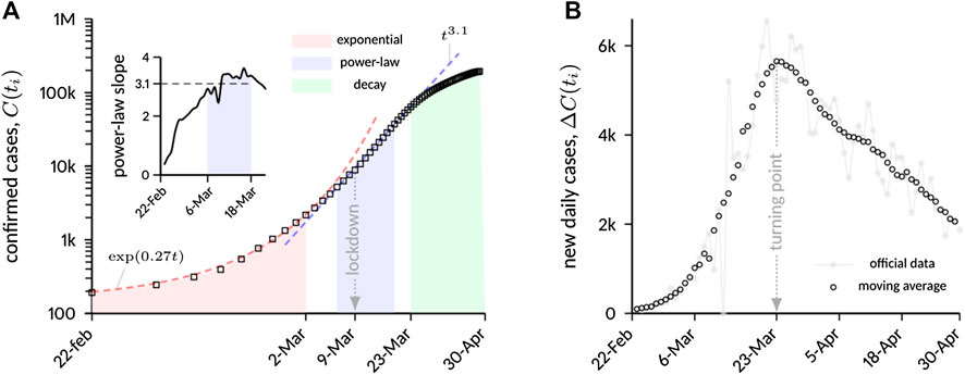
FIGURE 1. (A) Cumulative number of laboratory-confirmed COVID-19 infections in Italy. A moving average with a time window of 7 days was applied to the data to filter weekly fluctuations in case reporting. After an initial exponential growth, on March 6 the increase starts to follow a scaling law $t^{\alpha }$ with average $\overline{\alpha }\approx 3.1$. (B) Number of new daily cases of laboratory-confirmed COVID-19 infections in Italy. The turning point is highlighted. Gray circles represent official data, highlighting fluctuations in data reporting, while black circles were obtained with a 7-days moving average.

Evidence of algebraic growth has been observed and described elsewhere for other countries, including China [14] as well as other European countries [15], with exponents generally ranging from 2 to 4. From a fundamental perspective, this behavior has been attributed to structural changes in the topology of the population network that supports the epidemic spreading. Several authors [15, 16] have resorted to the small-world hypothesis [17] to justify the algebraic growth. More in general, spatial networks where short links are favored over long-range connections have been shown to produce power-law exponents in close similarity with the observed COVID-19 dynamics [18]. Similarly, the asymmetric decay has been put into some (empirical) connection with the simultaneous presence of a persistent phase of algebraic growth, in contrast with other countries where the epidemic has been characterized by a rather symmetric rise-and-fall behavior [19]. In this regard, graphs with a power-law degree distribution are known to produce outbreaks characterized by a polynomial growth followed by an exponential decay [20]. A functional form of this type was successfully used to fit COVID-19 data from over 100 countries [21], supporting the evidence that the nature of the underlying network is key to the infectious dynamics, and that growth and decay of the epidemic are indeed intimately connected. Network effects and their relationship with COVID-19 epidemic trends are further discussed in Ref. 22.

The reported observations have important consequences on traditional modeling approaches. From the perspective of classical population growth models, standard logistic models appear to be inappropriate, as they provide symmetric S-shaped curves for the cumulative number of infections; in contrast, the generalized Richard’s model (GRM) has been shown to provide a rather accurate description of the epidemic in Chinese provinces [8]. While the GRM can provide sub-exponential growth and asymmetric decline [23], it is known to lack clear epidemiological significance [24]. Compartment models are richer in terms of physics and allow addition of several degrees of freedom. The basic version of the celebrated Susceptible–Infectious–Removed (SIR) framework [25] can be easily transformed, under mild assumptions, into a logistic model [26], therefore suffering from the same above-mentioned limitations. Several refined SIR-like approaches have been proposed, particularly aiming at quantifying undetected cases [27] and at modeling the effect of containment policies [14, 28]. These have been modeled in most cases by means of a piecewise constant transmission rate (or, alternatively, by changing the local reproduction number) [29], or possibly by incorporating the effects of individual reaction [30].

Reconciling algebraic growth with mean-field models is not straightforward. Recently Ref. 21, observed that a general solution of the type $I\left(t\right)\propto t^{\alpha }$, where I is the infectious compartment, is compatible with a SIR model provided that the corresponding basic reproduction number decays as $t^{-1}$. On the other hand, Maier and Brockmann [14] (M&B hereinafter) have found, and proved analytically, that a region of algebraic growth can be captured by a slightly modified SIR-like model that includes a (constant) depletion rate of susceptible individuals. The question arises whether such a modeling framework is able to capture a markedly asymmetric decay dynamics such as the one occurring in Italy.

We conjecture that the three phases reported above are inherently coupled by endogenous epidemic processes, and thus they can be accurately modeled into a unique framework that relies exclusively on physics-based assumptions and policy-driven changes of the model parameters. Inspired by M&B, we aim to propose a compartment model that is able to: 1) capture the power-law growth; 2) generate an asymmetric decay; 3) incorporate unreported cases.

3. Proposed Compartment Model

We propose a compact compartment model of SEIQR-type (Susceptible–Exposed–Infectious–Quarantined–Removed), whose schematic is shown in Figure 2. Although many more compartments can be added to increase the level of detail and supposedly the realism of the model, we rather opted for a parsimonious framework, while focusing primarily on the reproduction of the observed scaling laws. We note explicitly that the inclusion of the Q-compartment is highly warranted for countries characterized by strong government interventions, since identified infectious individuals are typically quarantined and therefore they are no longer able to spread the disease. On the contrary, the necessity of taking the incubation period into account via the E-class is currently debated, mainly due to incomplete understanding of the relationship between incubation and latency periods for SARS-CoV-2 infection. However, a certain time lag between infection and infectiousness (in either clinical or subclinical cases) has often been observed [2, 31]; therefore, we chose to include the exposed class with an average incubation period ${\gamma }^{-1}$.

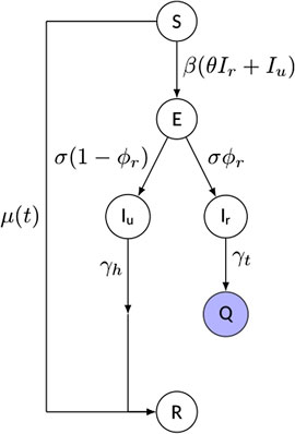
FIGURE 2. Schematic of the model and of its parameters (see text for details). The “quarantined” variable $Q\left(t\right)$ coincides, by construction, with the time-series of official laboratory-confirmed infections $C\left(t_i\right)$, when evaluated at the same sample points; $Q\left(t\right)$ is thus the only known variable in the context of a data-driven calibration of the model.

Additional key features of the model include:

• a time-dependent rate of depletion of the susceptible population, $\mu \left(t\right)$. Following M&B, we conjecture that starting (roughly) from the implementation of lockdown measures, and due to increased perception of the disease, a fraction of the S-class becomes unsusceptible due to self-protection, isolation, and adoption of preventive measures (e.g., wearing masks, hand-washing, etc.). However, and importantly, preliminary tests showed that a constant rate of depletion leads to strong under-prediction of the number of infections during the decay phase. Here we propose a time-dependent, decaying rate of depletion of susceptible individuals,

where ${\mu }_0$ is the initial rate of the depletion, $t^{\ast }$ is the start of the containment measures and τ is a timescale parameter. Such a modeling paradigm allows for a non-zero asymptotic residual of susceptible individuals, and is an essential component for capturing the strongly asymmetric behavior observed for the curve of new daily cases;

• an explicit distinction between reported and unreported cases. The infectious class has been split into reported (I_r) and unreported (I_u) individuals, modulated by a reporting rate ${\varphi }_r$. Since the policy in Italy consists into testing only symptomatic individuals, it is reasonable to assume that reported and unreported cases roughly coincide with asymptomatic (i.e., subclinical) and symptomatic (i.e., seeking medical attention) cases. Therefore, individuals belonging to the I_r class are infectious as long as they are tested and quarantined at a rate ${\gamma }_t$, and thus transferred to the Q-class. By construction, the variable $Q\left(t\right)$ coincides with the time-series of laboratory-confirmed infections $C\left(t_i\right)$. On the other hand, for individuals belonging to the Iu class, the disease goes unrecognized and they continue mixing with the susceptible population, before spontaneously recovering at a rate ${\gamma }_h$. We assume a bilinear transmission rate for reported and unreported cases: $\theta \beta$ for symptomatic individuals, and β for subclinical ones, with $\theta \in \left[\mathrm{0,1}\right]$. Although counter-intuitive, this choice was driven by the fact that people with symptoms that are severe enough to require medical attention are likely to reduce social contacts, therefore diminishing their transmission rate with respect to asymptomatic individuals (despite having, supposedly, a higher viral load and thus contagious potential).

Note that, for the sake of simplicity, we do not explicitly model the subsequent recovery/death of quarantined individuals, nor we distinguish between hospitalized and home-isolated patients; however, information in this regard can be inferred a-posterior once the temporal dynamics of $Q\left(t\right)$ and $I\left(t\right)$ is known. It is also worth to underline that the removed (R) class contains both recovered (from the unreported compartment) and protected individuals. Possible re-infection is not modeled as it is currently considered to be unlikely [32].

In summary, the temporal dynamics of the compartments is governed by the following system of ordinary differential equations:

where $s=S/N$ and N is the total (constant) population. The time dependency of the main variables has been omitted at the right-hand sides for the sake of clarity. All the parameters appearing in the model are constant and positive real numbers, with $\theta ,{\varphi }_r\in \left[\mathrm{0,1}\right]$, except for $\mu \left(t\right)$ that has explicit dependence on time. The basic reproduction number $R_0$ of this model can be inferred by a next-generation matrix approach; following [33]; the matrices F and V can be defined as

and $R_0$ is the spectral radius of $F{V}^{-1}$, yielding

The model defined by Eq. 3 has eight free parameters; some of them can be set a-priori based on epidemiological, clinical or policy-related evidence. The incubation time ${\sigma }^{-1}$ has been found by different clinical groups to be around 5 days [2, 31], thereby yielding $\sigma =1/5$, a value also used in similar modeling studies [34, 35]. The rate of testing ${\gamma }_t$ is country-specific; in Italy, the “Istituto Superiore di Sanità” (ISS) has reported an average time from symptoms onset to diagnosis (via pharyngeal swab) of 5 days, within the time range considered in this work. The infection duration in subclinical cases without medical treatment has been estimated to be in the range of 5–10 days [36]; after preliminary sensitivity tests, we set ${\gamma }_h=1/5$. The starting time of the susceptible population removal $t^{\text{*}}$ is expected to coincide roughly with the starting time of national lockdown; we left, however, $t^{\text{*}}$ as a free parameter for manual calibration.

4. Results and Discussion

Numerical simulations of the outbreak in Italy were obtained upon integration of Eq. 3 for the time range from February 24 to June 30, 2020. Table 1 summarizes the values of the entire set of model parameters, including those assigned a-priori and the ones inferred from the data. After several preliminary tests aimed to circumvent overfitting issues, we chose to optimize the parameter space containing $\left\{\beta ,\theta ,{\mu }_0,\tau ,E\left(0\right)\right\}$, while ${\varphi }_r$ and $t^{\text{*}}$ were left free to be manually varied in a parametric way until an optimal fit was found. The optimization procedure was carried out using an interior-point method implemented in MATLAB (Mathworks, Natick, United States); the optimization target was based on a blend of the cumulative number of confirmed cases and the daily number of new cases, that were weighted 10 and 90%, respectively. The infectious compartments were initialized as follows: $I_r\left(0\right)={\varphi }_{r}E\left(0\right)$, $I_u\left(0\right)=\left(1-{\varphi }_r\right)E\left(0\right)$, while the other initial conditions are either known from data or can be found by subtraction, with $N=60\times {10}^6$.

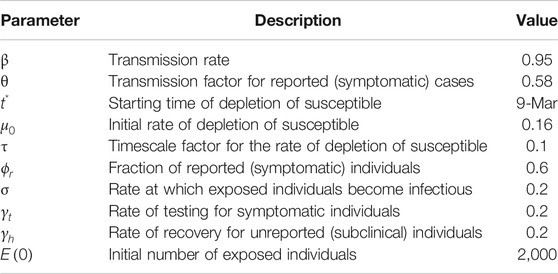
TABLE 1. Optimal values of the estimated model parameters for the simulation of the outbreak in Italy.

Main results are shown in Figure 3. Figure 3A reports the temporal evolution of $Q\left(t\right)$, as compared with the time-series of laboratory-confirmed infections $C\left(t_i\right)$. The agreement is very good for all the phases of the outbreak. Interestingly, the best-fit value for $t^{\text{*}}$ was March 9, i.e., the start of the national quarantine, which indirectly proves the robustness of the proposed framework in reproducing the underlying epidemic mechanisms at play. The inset of Figure 3A reports the power-law slope provided by the model, which is in very good agreement with the observed one, proving that the model is capable of reproducing the peculiar algebraic growth phase of the COVID‐19 pandemic reported in several countries.

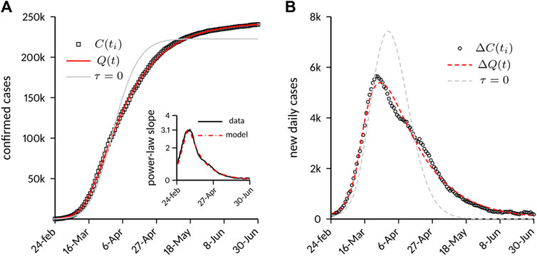
FIGURE 3. Case numbers in Italy compared to model predictions. (A) Cumulative number of laboratory-confirmed infections. The model predictions are shown both with the full model and with a variant obtained by setting $\tau =0$ (constant depletion rate of the susceptible population). The inset reports the local power-law slope for the moving-averaged official data and the full-model prediction. (B) Number of new daily cases.

Of note, the model was able to capture the decay phase of the epidemic correctly without any further change of the parameters. This circumstance suggests a strong link between the decay dynamics and the timing and implementation of the containment strategies. It is conjectured that an incomplete depletion of the susceptible population during the lockdown (provided by the exponential decay of $\mu \left(t\right)$) naturally sets the observed slow decay. It can be further hypothesized in light of the results that the behavioral changes established during the containment phase persist throughout the subsequent phases of the epidemic. Since lower values of the timescale τ over which the susceptible removal occurs yield a faster decay, this parameter be re-interpreted as an “effectiveness index” of the implementation of containment policies.

We also tested a variant of the model that more closely resembles the original M&B approach, with a constant depletion rate of the susceptible population $\mu ={\mu }_0$. Upon re-running the optimization procedure with $\tau =0$, we obtained similar values as those reported in Table 1, but it was not possible to match the decay phase correctly. This variant of the model provides a reasonable agreement only up to the turning point of the epidemic (with the peak value of new daily cases highly over-estimated), while strongly under-estimating the number of infections during the decay phase, as clearly seen in Figure 3B. An additional steep change of the model parameters would be necessary, although this would be hardly justifiable in terms of physical assumptions or containment policies.

In light of the above mentioned results and observations, it is instructive to directly quantify the effects of $\mu \left(t\right)$ on the epidemic dynamics. To this aim, it is worth to preliminarily observe that, under a disease-free linearization (i.e., assuming that containment dominates over infection) the normalized number of susceptible for $t\gg t^{\ast }$ is not null (as in the case $\tau =0$) but converges to

showing that τ is explicitly responsible for the incomplete removal. Although it is possible, in principle, to derive a closed-form expression for $Q\left(t\right)$ under some mild simplifying hypotheses, the analytic treatment becomes very involved and it is cumbersome to extract immediate information. The reader is referred to Ref. 14 for an analytic demonstration of how the depletion of susceptible is responsible for the power-law growth, while the effects of ${\mu }_0$ and τ on the decay are best revealed through parametric analysis. Figure 4 shows the effects of the containment-related parameters on $\text{Δ}Q$, with the other modeling parameters being held equal to the optimal solution reported in Table 1. Figure 4A shows that lower values of ${\mu }_0$ (i.e., weaker depletion) tend to shift the curve toward higher values of $\text{Δ}Q$ and delay the turning point, while the overall shape is roughly preserved. On the other hand, Figure 4B demonstrates that values of $\tau >0$ contribute to asymmetrize the curve of new daily cases, effectively slowing the decay while preserving the growth dynamics. Since τ is directly related to the residual number of susceptible individuals during the course of the epidemic, see Eq. 6, these findings reinforce our claim that the observed asymmetry is directly related to a (spatially-averaged) incomplete depletion of the susceptible population during the containment phase.

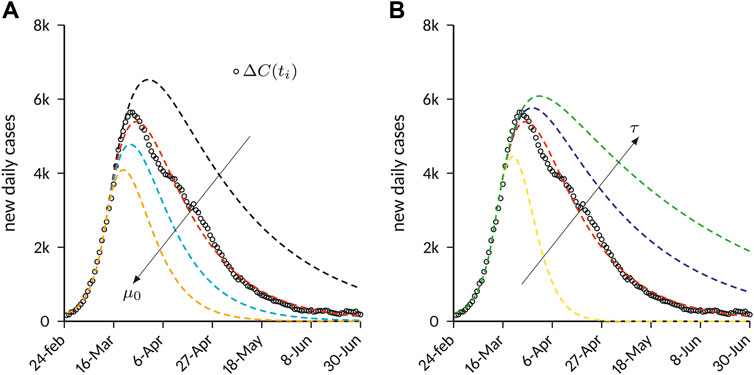
FIGURE 4. Effects of containment on the number of new daily cases predicted by the SEIQR compartment model. The results are obtained with the parameters provided in Table 1, and by varying the parameters ${\mu }_0$ and τ. The red curve corresponds to the optimal solution. Moving-averaged official data are also reported. (A) Effect of ${\mu }_0$ for values in the set $\left[0.14,0.16,0.18,0.22\right]$. (B) Effect of τ for values in the set $\left[0.0,0.1,0.12,0.13\right]$.

With regards to the functional form of the time-varying depletion rate $\mu \left(t\right)$, the exponential decay was chosen as the most natural one with a clear and intuitive biological significance. However, we also explored whether alternative expressions for $\mu \left(t\right)$ are able to reproduce the essential characteristics of the COVID-19 epidemic. To this end, we consider a simplified version of the proposed compartment model, wherein the E-class is removed and ${\varphi }_r=\theta =1$, i.e., all infected individuals are identified and quarantined:

In such case, assuming that in a certain time interval $Q\left(t\right)\approx t^{\alpha }$, and that containment dominates over infection, simple analytic manipulations yield

where $c_1$ and $c_2$ are constants. We tested the behavior of the complete model by plugging Eq. 8 into Eq. 3; we were able to generate outbreaks (not shown here) in good agreement with the official data and for similar values of the model parameters as those reported in Table 1. While this circumstance promotes the correctness of the underlying modeling hypotheses, additional tests and analyses are required to determine which functional form is most suitable for $\mu \left(t\right)$, and whether other decay laws (e.g., Gaussian) can be instead ruled out to describe the containment process.

The role of subclinical infected with regards to the spread of the disease is one of the most debated epidemiological and biomedical issues in the context of the COVID-19 outbreak [37]. Accurate studies in small-scale, “laboratory-like” contexts with blanket testing showed that a substantial fraction of SARS-CoV-2-positive individuals can display very mild symptoms or even remain completely asymptomatic throughout the course of the infection, while having a viral load comparable to that of symptomatic patients [38–40]. Here we found a very good fit for values of the reporting rate in the range ${\varphi }_r\in \left[0.55,0.65\right]$, yielding a fraction of unreported (subclinical) cases $\left(1-{\varphi }_r\right)$ in line with previous modeling and experimental estimates [27, 38].

It is worth to remark, in general, that we were able to generate outbreaks in good agreement with official data for a certain range and combination of the model parameters. While we did not quantify sensitivity, nor we carried out specifical statistical analyses of the confidence interval of such parameters, we chose the set of values that yielded the best accordance with the observed scaling laws (exponential growth rate, peak power-law slope, decay dynamics) and a reasonable value for the basic reproduction number. For the best-fit reported in Table 1, we get $R_0=3.53$, very much in line with previous literature results [41].

5. Concluding Remarks

In this study, we started from the preliminary observation that in countries such as Italy, the cumulative number of infections displays an initial exponential amplification, followed by a power-law growth and a markedly asymmetric saturation behavior. We conjecture that these three phases are intimately connected and can be described by the interplay between the contagion process and the behavioral changes/containment policies acting on the population over comparable time scales.

Based on this hypothesis, and inspired by previous work by Ref. 14, we proposed a SEIQR-type compartment model with the following salient features: i) a compartment for unreported (asymptomatic) infected, that are supposed to play a major role in the spread of the disease; ii) a time-dependent rate of depletion of the susceptible population, which allows for a non-zero asymptotic residual of susceptible individuals.

The model was able to accurately reproduce the entire epidemic course in Italy, including quantitative agreement with exponential growth and power-law slope, for a plausible range of the model free parameters, with only one steep change of the parameters driven by the introduction of strict containment strategies. This circumstance suggests that the timing and implementation of containment policies (as quantified by model parameters $t^{\text{*}}$, ${\mu }_0$ and τ) may effectively establish the decay characteristics of the epidemic. In particular we conjecture that the slow decay of the Italian epidemic can be attributed to an incomplete depletion of susceptible individuals during the containment phase.

The proposed modeling framework could be profitably used to gain insights and predictions on the so-called “second wave” of the epidemic, which (as of early October 2020) appears to be hitting Italy and other countries. To this purpose, the model could be modified by 1) introducing a release rate of protected individuals (from compartment R to S), that reflects the relaxation of containment measures as well as the gradually diminished perception of the pandemic; 2) accounting for a different testing policy: while only symptomatic individuals were tested during the first wave of the epidemic, the introduction of contact tracing and screening procedures has certainly contributed to increase the reporting rate ${\varphi }_r$, whereas the simultaneous improvements in testing efficiency and COVID-related infrastructures has led to a decrease in the testing time ${\varphi }_t$.

This study presents a number of simplifications and limitations that, however, do not affect the main conclusions. Among others, the number of confirmed infections is influenced by the number of tests performed each day, an aspect that was only weakly incorporated into the model via the (constant) fraction of reported cases ${\varphi }_r$. Even though many countries experienced initial difficulties with the testing capacity, the robustness and universality of the observed epidemic trends [19] strongly suggest that the scaling laws at play are primarily driven by the described containment-related mechanisms, with the scale of testing playing a minor role in the process [22]. Furthermore, the COVID-19 pandemic has been shown to have a strong geographical character with localized outbreaks, due to so-called superspreaders or family clusters [42]. In the context of a well-mixed framework, such as the one proposed in this paper, this phenomenon could be modeled by considering a specific infectious compartment with a much higher transmission rate, similarly as in Ref. 43. This aspect was not accounted for here and is left for future work.

Data Availability Statement

The raw data supporting the conclusions of this article will be made available by the authors, without undue reservation.

Author Contributions

FC designed the study, conducted the data analysis, developed the mathematical model, interpreted the data and wrote the article.

Conflict of Interest

The authors declare that the research was conducted in the absence of any commercial or financial relationships that could be construed as a potential conflict of interest.

Acknowledgments

The author is indebted to Valerio Carandente, Marco Cozzo, Vincenzo Di Savino and Andrea Piccolo for insightful discussions.

References

1. Zhu N, Zhang D, Wang W, Li X, Yang B, Song J, et al. A novel coronavirus from patients with pneumonia in China, 2019. N Engl J Med (2020). 382:727–33. doi:10.1056/NEJMoa2001017
2. Li Q, Guan X, Wu P, Wang X, Zhou L, Tong Y, et al. Early transmission dynamics in Wuhan, China, of novel coronavirus-infected pneumonia. N Engl J Med (2020). 382:1199–207. doi:10.1056/NEJMoa2001316
3. Wu F, Zhao S, Yu B, Chen Y-M, Wang W, Song Z-G, et al. A new coronavirus associated with human respiratory disease in China. Nature (2020). 579:265–9. doi:10.1038/s41586-020-2008-3
5.World Health Organization. Coronavirus disease 2019 (COVID-19) weekly epidemiological update—5 october 2020 (2020). https://www.who.int/publications/m/item/weekly-epidemiological-update---5-october-2020.
6. Adam D. Special report: the simulations driving the world's response to COVID-19. Nature (2020). 580:316–8. doi:10.1038/d41586-020-01003-6
7. Shen CY. Logistic growth modelling of COVID-19 proliferation in China and its international implications. Int J Infect Dis (2020). 96:582–9. doi:10.1016/j.ijid.2020.04.085.
8. Wu K, Darcet D, Wang Q, Sornette D. Generalized logistic growth modeling of the COVID-19 outbreak in 29 provinces in China and in the rest of the world (2020). arXiv preprint arXiv:2003.05681.
9. Prem K, Liu Y, Russell TW, Kucharski AJ, Eggo RM, Davies N, et al. The effect of control strategies to reduce social mixing on outcomes of the COVID-19 epidemic in Wuhan, China: a modelling study. Lancet Public Health (2020). 5:e261–70. doi:10.1016/S2468-2667(20)30073-6
10. Jit A, Russell T, Diamond C, Liu Y, Edmunds J, Funk S, et al. Early dynamics of transmission and control of COVID-19: a mathematical modelling study. Lancet Infect Dis (2020). 20:P553–8. doi:10.1016/S1473-3099(20)30144-4
11. Jewell NP, Lewnard JA, Jewell BL. Predictive mathematical models of the COVID-19 pandemic. J Am Med Assoc (2020). 323:1893–4. doi:10.1001/jama.2020.6585
12. Ministero della Salute (2020). COVID‐19 weekly monitoring reportAvailable from: http://www.salute.gov.it/nuovocoronavirus (Accessed July 6, 2020).
13. Dong E, Du H, Gardner L. An interactive web-based dashboard to track COVID-19 in real time. Lancet Infect Dis (2020). 20:533–4. doi:10.1016/S1473-3099(20)30120-1
14. Maier BF, Brockmann D. Effective containment explains subexponential growth in recent confirmed COVID-19 cases in China. Science (2020). 368:742–6. doi:10.1126/science.abb4557
15. Manchein C, Brugnago EL, da Silva RM, Mendes CFO, Beims MW. Strong correlations between power-law growth of COVID-19 in four continents and the inefficiency of soft quarantine strategies. Chaos (2020). 30:041102. doi:10.1063/5.0009454
17. Watts DJ, Strogatz SH. Collective dynamics of 'small-world' networks. Nature (1998). 393:440–2. doi:10.1038/30918
18. Medo M. Contact network models matching the dynamics of the COVID-19 spreading (2020). arXiv preprint ArXiv:2003.13160.
19. Singer HM. The COVID-19 pandemic: growth patterns, power law scaling, and saturation. Phys Biol (2020). 17(5):055001. doi:10.1088/1478-3975/ab9bf5
20. Vazquez A. Polynomial growth in branching processes with diverging reproductive number. Phys Rev Lett (2006). 96:038702. doi:10.1103/physrevlett.96.038702
21. Bodova K, Kollar R. Emerging algebraic growth trends in SARS-CoV-2 pandemic data. Phys Biol (2020). 20:42. doi:10.1088/1478-3975/abb6db
22. Thurner S, Klimek P, Hanel R. A network-based explanation of why most COVID-19 infection curves are linear. Proc Natl Acad Sci USA (2020). 117:22684–9. doi:10.1073/pnas.2010398117
23. Chu KH. Fitting the Gompertz equation to asymmetric breakthrough curves. J Environ Chem Eng (2020). 8:103713. doi:10.1016/j.jece.2020.103713
24. Li J, Lou Y. Characteristics of an epidemic outbreak with a large initial infection size. J Biol Dynam (2016). 10:366–78. doi:10.1080/17513758.2016.1205223
25. Kermack WO, McKendrick AG. A contribution to the mathematical theory of epidemics. Proc Roy Soc Lond (1927). 115:700–21. doi:10.1098/rspa.1927.0118
26. Postnikov EB. Estimation of COVID-19 dynamics “on a back-of-envelope”: does the simplest SIR model provide quantitative parameters and predictions? Chaos Solit Fractals (2020). 135:109841. doi:10.1016/j.chaos.2020.109841
27. Li R, Pei S, Chen B, Song Y, Zhang T, Yang W, et al. Substantial undocumented infection facilitates the rapid dissemination of novel coronavirus (SARS-CoV-2). Science (2020). 368:489–93. doi:10.1126/science.abb3221
28. Hellewell J, Abbott S, Gimma A, Bosse NI, Jarvis CI, Russell TW, et al. Feasibility of controlling COVID-19 outbreaks by isolation of cases and contacts. Lancet Global Health (2020). 8:e488–96. doi:10.1016/S2214-109X(20)30074-7
29. Munday G, Blanchini F, Bruno R, Colaneri P, Di Filippo A, Di Matteo A, et al. Modelling the COVID-19 epidemic and implementation of population-wide interventions in Italy. Nat Med (2020). 26:855–60. doi:10.1038/s41591-020-0883-7
30. Lin Q, Zhao S, Gao D, Lou Y, Yang S, Musa SS, et al. A conceptual model for the coronavirus disease 2019 (COVID-19) outbreak in Wuhan, China with individual reaction and governmental action. Int J Infect Dis (2020). 93:211–6. doi:10.1016/j.ijid.2020.02.058
31. Lauer SA, Grantz KH, Bi Q, Jones FK, Zheng Q, Meredith HR, et al. The incubation period of coronavirus disease 2019 (COVID-19) from publicly reported confirmed cases: estimation and application. Ann Intern Med (2020). 172:577–82. doi:10.7326/M20-0504
32. Deng W, Bao L, Liu J, Xiao C, Liu J, Xue J, et al. Primary exposure to SARS-CoV-2 protects against reinfection in rhesus macaques. Science (2020). 369:818–23. doi:10.1126/science.abc5343
33. Lv P, Watmough J. Reproduction numbers and sub-threshold endemic equilibria for compartmental models of disease transmission. Math Biosci (2002). 180:29–48. doi:10.1016/S0025-5564(02)00108-6
34. Sun G-Q, Wang S-F, Li M-T, Li L, Zhang J, Zhang W, et al. Transmission dynamics of COVID-19 in Wuhan, China: effects of lockdown and medical resources. Nonlinear Dynam (2020). 16:1–13. doi:10.1007/s11071-020-05770-9
35. Li M-T, Sun G-Q, Zhang J, Zhao Y, Pei X, Li L, et al. Analysis of COVID-19 transmission in Shanxi Province with discrete time imported cases. Math Biosci Eng (2020). 17:3710–20. doi:10.3934/mbe.2020208
36. Li Y, Yao L, Wei T, Tian F, Jin D-Y, Chen L, et al. Presumed asymptomatic carrier transmission of COVID-19. J Am Med Assoc (2020). 323:1406–7. doi:10.1001/jama.2020.2565
37. Wang M, Yokoe DS, Havlir DV. Asymptomatic transmission, the Achilles’ heel of current strategies to control COVID-19. N Engl J Med (2020). 382:2158–60. doi:10.1056/NEJMe2009758
38. Lavezzo E, Franchin E, Ciavarella C, Cuomo-Dannenburg G, Barzon L, Del Vecchio C, et al. Suppression of a SARS-CoV-2 outbreak in the Italian municipality of Vo′. Nature (2020). 584, 425–9. doi:10.1038/s41586-020-2488-1
39. Mizumoto K, Kagaya K, Zarebski A, Chowell G. Estimating the asymptomatic proportion of coronavirus disease 2019 (COVID-19) cases on board the Diamond Princess cruise ship. Euro Surveill (2020). 25:2000180. doi:10.2807/1560-7917.ES.2020.25.10.2000180
40. Russell TW, Hellewell J, Jarvis CI, van Zandvoort K, Abbott S, Ratnayake R, et al. Estimating the infection and case fatality ratio for coronavirus disease (COVID-19) using age-adjusted data from the outbreak on the Diamond Princess cruise ship, February 2020. Euro Surveill (2020). 25:200256. doi:10.2807/1560-7917.ES.2020.25.12.2000256
41. Flasche M, Bertuzzo E, Mari L, Miccoli S, Carraro L, Casagrandi R, et al. Spread and dynamics of the COVID-19 epidemic in Italy: effects of emergency containment measures. Proc Natl Acad Sci USA (2020). 117:10484–91. doi:10.1073/pnas.2004978117
42. Rinaldo Y, Eggo RM, Kucharski AJ. Secondary attack rate and superspreading events for SARS-CoV-2. Lancet (2020). 395:e47. doi:10.1016/s0140-6736(20)30462-1
Keywords: COVID-19, power-law growth, compartment model, containment strategies, unreported cases
Citation: Capuano F (2020) Modeling Growth, Containment and Decay of the COVID-19 Epidemic in Italy. Front. Phys. 8:586180. doi: 10.3389/fphy.2020.586180
Received: 22 July 2020; Accepted: 30 October 2020;
Published: 30 November 2020.
Edited by:
Zhen Wang, Hong Kong Baptist University, Hong KongReviewed by:
Matúš Medo, University of Electronic Science and Technology of China, ChinaGui-Quan Sun, North University of China, China
Copyright © 2020 Capuano. This is an open-access article distributed under the terms of the Creative Commons Attribution License (CC BY). The use, distribution or reproduction in other forums is permitted, provided the original author(s) and the copyright owner(s) are credited and that the original publication in this journal is cited, in accordance with accepted academic practice. No use, distribution or reproduction is permitted which does not comply with these terms.
*Correspondence: Francesco Capuano, francesco.capuano@unina.it