Unravelling the Impacts of Parameters on Surrogate Safety Measures for a Mixed Platoon

Abstract

With the precedence of connected automated vehicles (CAVs), car-following control technology is a promising way to enhance traffic safety. Although a variety of research has been conducted to analyze the safety enhancement by CAV technology, the parametric impact on CAV technology has not been systematically explored. Hence, this paper analyzes the parametric impacts on surrogate safety measures (SSMs) for a mixed vehicular platoon via a two-level analysis structure. To construct the active safety evaluation framework, numerical simulations were constructed which can generate trajectories for different kind of vehicles while considering communication and vehicle dynamics characteristics. Based on the trajectories, we analyzed parametric impacts upon active safety on two different levels. On the microscopic level, parameters including controller dynamic characteristics and equilibrium time headway of car-following policies were analyzed, which aimed to capture local and aggregated driving behavior’s impact on the vehicle. On the macroscopic level, parameters incorporating market penetration rate (MPR), vehicle topology, and vehicle-to-vehicle environment were extensively investigated to evaluate their impacts on aggregated platoon level safety caused by inter-drivers’ behavioral differences. As indicated by simulation results, an automated vehicle (AV) suffering from degradation is a potentially unsafe component in platoon, due to the loss of a feedforward control mechanism. Hence, the introduction of connected automated vehicles (CAVs) only start showing benefits to platoon safety from about 20% CAV MPR in this study. Furthermore, the analysis on vehicle platoon topology suggests that arranging all CAVs at the front of a mixed platoon assists in enhancing platoon SSM performances.

1. Introduction

Traffic safety, as a global issue, has been drawing considerable concentration from the public during the past decades. Among all collisions, rear-end collisions are the most frequently occurring type [1]. Generally, rear-end crashes happen due to improper vehicular longitudinal single-lane motions. With the rapid and continuous development of sensing and communication technologies, connected automated vehicles (CAVs) equipped with on-board sensors and wireless communication devices provides unprecedented opportunities to drastically improve traffic safety [2,3,4]. For a CAV, cooperative adaptive cruise control (CACC) is a predominant approach to deal with inter-vehicle longitudinal driving behaviors by applying detected parameters from the preceding vehicle and real-time information received via vehicle-to-vehicle (V2V) communication. However, CACC can lose cooperation and degrade to ACC, owing to the incomplete information caused by both receivers (such as communication failure during transmission) or senders (such as a human driven vehicles (HDVs) without sending functions) [5,6]. Notably, communication degradation can affect a vehicle’s car-following behaviors and safety.

In the past, traditional HDV rear-end crash analysis and evaluation mainly focused on historical accidents and their severity through some statistical models [7,8,9,10]. These after-crash studies belong to the field of passive safety, endeavoring to reduce harm and damage from accidents that have occurred. Nevertheless, passive safety has lots of drawbacks, such as a long observation period and small sampling size. One of the most significant disadvantages is that it fails to catch safety characteristics of vehicle’s driving behavior and state at a certain moment. In light of this, active safety technologies aiming at preventing accidents are emerging, which are more efficient and meet with CAV’s demand for real-time safety analysis. Much literature has focused on the active safety evaluation to study the CACC/ACC rear-end crash risk. Some risk prediction and evaluation models, such as references [11,12,13,14] were proposed, applying macroscopic traffic flow data including density, volume, etc., to proactively perceive potential risk. For example, reference [15] attempted to utilize different driver assistance systems to better reduce small-scale inclement weather-caused rear-end crashes. Two disturbance-based indices were then proposed in order to represent the general safety level of car-following scenarios [16]. These methods are useful but neglect important microscopic traffic characteristics that are also accountable for collision. Therefore, surrogate safety measures (SSMs) that usually uses the follower’s acceleration, velocity, and spacing with the leading vehicle to identify the potential collision dangers between vehicles has gained increasing interests to quantify safety. Among all SSMs, time-to-collision (TTC) has been widely applied in previous studies. Considering the limitation of TTC, some extension measures of TTC, such as time exposed time-to-collision (TET) and time-integrated time-to-collision (TIT) are proposed subsequently (i.e., [17,18,19,20]). A developed CACC strategy integrating a variable speed limit control was proved to effectively reduce rear-end crash risk via TTC-related SSMs, i.e., a 98% decline in TET and TIT [21].

The aforementioned discussions are based on the assumption of a full (connected) automated environment, however, even though the CAV technology is rapidly developing, achieving a pure CAV environment is still quite distant. Therefore, partially connected automated environments constructed by a mixture of CAVs and HDVs will be more realistic in the foreseeable future. Much work so far has focused on the impacts of CAV market penetration rate (MPR) on safety in different application scenarios. A surrogate safety assessment model including five SSMs was established, devoted to evaluating both segment and intersection crash risks under various CAV MPRs [22]. An investigation of the safety influences of CAV MPR at intersections with different signalization degrees was conducted using SSMs, in which the results showed a difference in SSM changing trend with low or high CAV penetration [23]. Furthermore, reference [24] pointed out that automated vehicles (AV) suffering from degradation can increase a mixed platoon’s rear-end crash risk. Although this research explores the impacts of some parameters for the CAV design, a systematic analysis of all parameters of concern is missing. Especially, these works do not fully consider the higher order effects caused by feedback and feedforward gains inside the CAV controllers, and the vehicle platoon topology’s impact and the corresponding communication degradation are largely missing.

Therefore, to fill the gap, this study aims to further unravel the parameter impacts on SSM under partially connected automated environment. To this end, a two-level active safety evaluation framework is proposed to perform a systematic parametric analysis. The novelty of this study lies in the cooperation of platoon topology formation and communication degradation. Another contribution is that we consider evaluating the impact of dynamic characteristics embedded in a decentralized linear CAV controller. The findings of this study can also be helpful for safety improvement and practical mixed traffic flow management.

The rest of this paper is organized as follows: Section 2 provides the overview of the two-level active safety framework of vehicle topology and car-following models for the mixed platoon under partial connected automated environment. Section 3 introduces the definitions of surrogated safety measures. Simulation experiments and discussion are conducted in Section 4. Section 5 draws the conclusion and gives some future directions. Finally, Section 6 discusses limitations and future works.

2. Materials and Methods

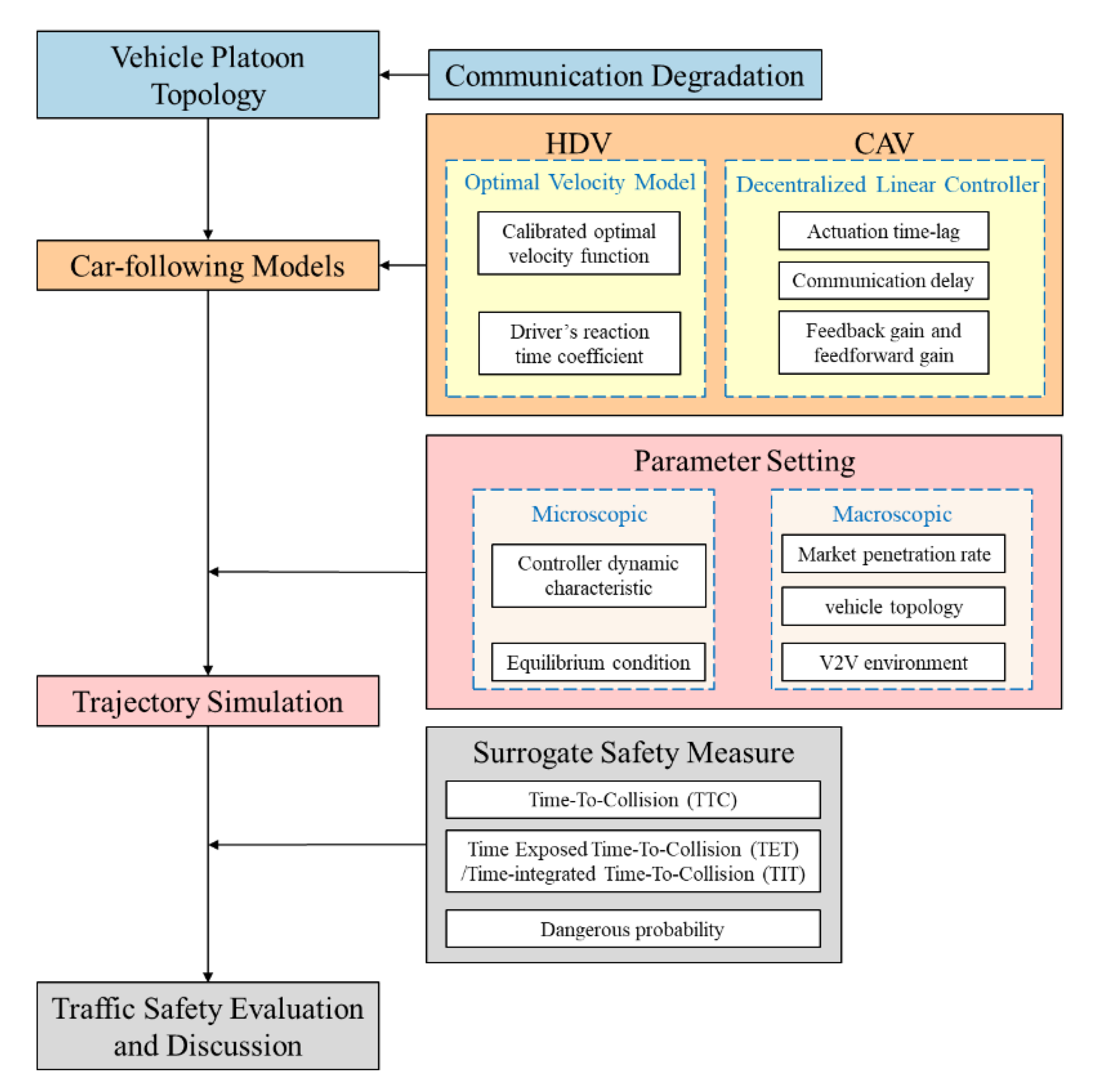
The overview of the proposed framework is shown in Figure 1, which has four parts: the vehicle platoon topology is responsible for dictating vehicle order and based on that, the corresponding car-following models for each car-following pair is picked to provide the longitudinal movement of CAVs and HDVs. By giving the first leading vehicle trajectory and car following models, a numerical simulation is conducted to generate each vehicle’s trajectory. By the trajectories for each vehicle inside the platoon, the traffic safety evaluation and discussion module gives the safety performances of input platoon trajectory data via SSM. More detailed explanations of each component are provided in the following sections. It is noteworthy that in the process of parameter setting, the microscopic level strives for capturing the parametric impacts of vehicle local and aggregated driving behavior on SSM, whereas the macroscopic level works towards parametric impacts of an aggregated platoon on SSM.

This section firstly describes the platoon’s vehicle topology formation under a partially connected automated environment considering communication degradation. For simplicity, other than CAV and HDV, we assumed that all AVs in the mixed platoon came from the degraded CAV. Furthermore, to describe the car-following behavior, models used for three different kinds of vehicles in the platoon are then proposed, respectively. After settling down the topology and car-following models, trajectories of a mixed platoon can be generated.

2.1. Mixed Platoon Topology Formation Considering Communication Degradation

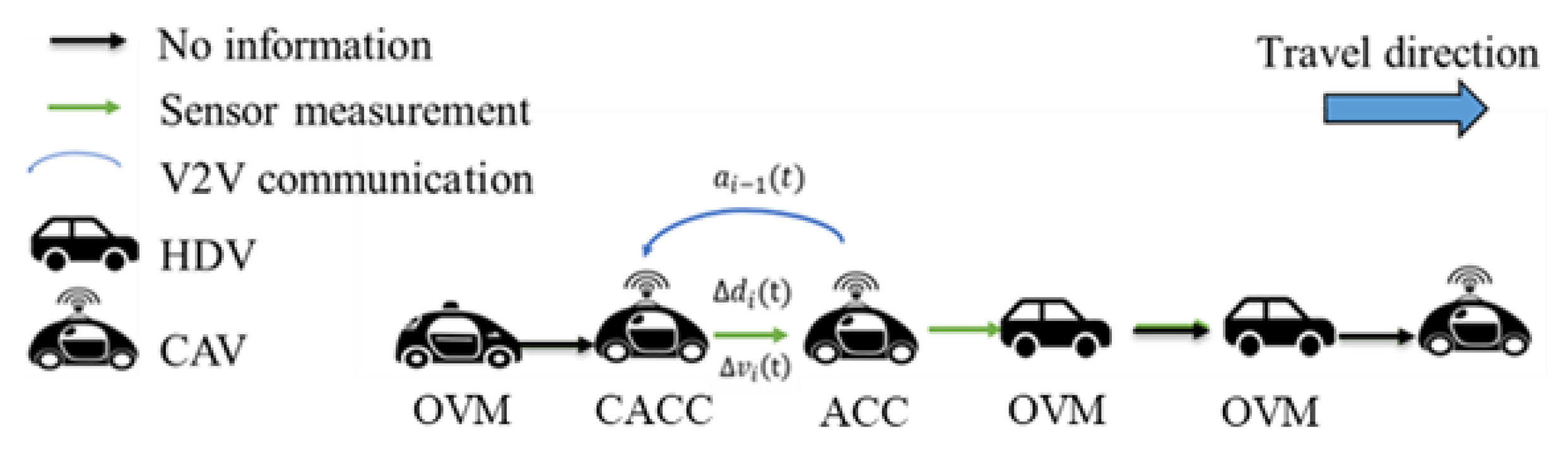
The communication topology in this study complies with the most widely acceptable one-vehicle look ahead (predecessor-following) style, in which a CAV can only receive the information from the most adjacent leading vehicle. We postulate that every CAV is equipped with V2V devices whereas the HDVs are not. Notice that communication degradation (hereinafter referred to as degradation) happens when the predecessor’s acceleration becomes unavailable for a CAV, i.e., it does not have an HDV leader. Thus, when degradation occurs, a CAV’s following mode degrades to ACC. Notably, although AVs fail to have V2V communication, they can still detect some information about the preceding vehicle through sensor measurement. Figure 2 illustrates the schematic of a mixed platoon’s car-following relationship.

2.2. HDV Car-Following Model

The optimal velocity model (OVM) is one of the most widely used HDV car-following models which can reproduce the realistic human drivers’ car-following behaviors in a decent manner [25]. OVM adjusts follower driving towards an optimal velocity which is defined as a function of time and headway. The optimal velocity function is calculated as:

$$v_n^{*}\left(\Delta s_n\left(t\right)\right)=v_0\left[\tanh \left(\frac{P_{n-1}\left(t\right)-P_n\left(t\right)-l_{n-1}}{b}-c_1\right)+c_2\right]$$

(1)

where $v_n^{*}$ is the optimal velocity, P_n−1(t) and P_n(t) is the position of vehicle n and n − 1 at t time, respectively. The time headway Δs_n(t) = P_n−1(t) − P_n(t) − l_n−1, where l_n−1 represents the length of predecessor. b is the unit scale.v₀, c₁, and c₂ are predefined coefficients. Then, OVM assumes the acceleration of the $n\mathrm{th}$ vehicle can be determined based on the velocity difference between the actual velocity and optimal velocity computed via Equation (1). A human driver is not able to respond to the preceding vehicle’s acceleration change immediately, therefore the driver’s reaction time coefficient τ_n is incorporated in the acceleration calculation, written as:

$$a_{n,OVM}\left(t\right)=\alpha \left[v_n^{*}\left(\Delta s_n\left(t-{\tau }_n\right)\right)-v_n\left(t-{\tau }_n\right)\right]$$

(2)

where α is a constant sensitive parameter. In order to make OVM more concrete, the optimal velocity function used in this paper applies the calibrated highway field data in reference [26], which can be described as:

$$v_n^{*}\left(\Delta s_n\left(t\right)\right)=16.8\left[\tanh 0.0860\left(\Delta s_n\left(t\right)-25\right)+0.913\right]$$

(3)

2.3. Decentralized Linear CAV/AV Controller

In this paper, we use the prominent linear decentralized controller proposed by [27] to model CAVs and AVs in a platoon, due to its simplicity and robustness against vehicle dynamics and communication delay uncertainties. It has also been validated via simulation that with proper parameter setting, this controller can provide efficient control with guaranteed string stability. To describe the system, a state space system is constructed by defining, the system state for CAV $i$ at time $t$ as $x_i\left(t\right)={\left[\mathsf{\Delta }{s}_i\left(t\right), \mathsf{\Delta }{v}_i\left(t\right),a_i\left(t\right)\right]}^T$, where the first item $\mathsf{\Delta }{s}_i\left(t\right)$ denotes the deviation from the equilibrium spacing following a constant time headway policy; $\mathsf{\Delta }{v}_i\left(t\right)$ is the relative speed with leader and $a_i\left(t\right)$ is the realized acceleration, and a control input is defined as the demanding acceleration denoted as $u_i\left(t\right)$. Based on the above, the state-space formulation of a CAV can be written as an ordinary differential equation given below:

$$\dot{x_i}\left(t\right)=A_i{x}_i\left(t\right)+B_i{u}_i\left(t\right)+D_i{a}_{i-1}\left(t\right)$$

(4)

where $A_i=\left[\begin{array}{ccc}0& 1& -t_i^{*}\\ 0& 0& -1\\ 0& 0& \frac{1}{{\phi }_i}\end{array}\right]$, $B_i=\left[\begin{array}{c}0\\ 0\\ \frac{1}{{\phi }_i}\end{array}\right]$, $D_i=\left[\begin{array}{c}0\\ 1\\ 0\end{array}\right]$, $t_i^{*}$ is desired time-gap for vehicle $i$, and ${\phi }_i$ is the actuation time-lag. $a_{i-1}\left(t\right)$ is the acceleration of the preceding vehicle acquired through V2V communication. To regulate the speed difference and deviation from equilibrium spacing, a linear feedback and feedforward controller is adopted:

$$u_i\left(t\right)=K{x}_i\left(t\right)+K_f{a}_{i-1}\left(t-\theta \right)$$

(5)

where feedback gain matrix $K$ is a predetermined coefficient matrix, $K=\left[k_s,k_v,k_a\right]$. $k_s$, $k_v$, $k_a$ are feedback gains corresponding to the deviation from the equilibrium spacing, relative speed and acceleration, respectively. $K_f$ is the feedforward gain responding to the predecessor’s acceleration, set $K_f=\left[k_f\right]$. Communication transmission between vehicles is not instantaneously, therefore $\theta$ is used to express the communication delay.

Combining Equations (4) and (5), the CAV’s dynamic characteristic can be reformulated as:

$$\dot{x_i}\left(t\right)=\left(A_i+B_{i}K\right)x_i\left(t\right)+D_i{a}_{i-1}\left(t\right)+B_i{K}_f{a}_{i-1}\left(t-\theta \right)$$

(6)

For ACC, degradation occurs. Therefore, feedforward control is inaccessible under this circumstance, set as $K_f=0$. The control input becomes:

$$u_i\left(t\right)=K{x}_i\left(t\right)$$

(7)

And state-space formulation for AV is:

$$\dot{x_i}\left(t\right)=\left(A_i+B_{i}K\right)x_i\left(t\right)+D_i{a}_{i-1}\left(t\right)$$

(8)

In summary, the acceleration of vehicle $i$ in the mixed platoon is developed as below:

$$a_i\left(t\right)=\{\begin{array}{ll}K{x}_i\left(t\right)+K_f{a}_{i-1}\left(t-\theta \right)& \hspace{1em}\mathrm{for} \mathrm{CAV}\\ \hspace{1em}K{x}_i\left(t\right)& \hspace{1em}\mathrm{for} \mathrm{AV}\\ \alpha \left[v_i^{*}\left(\mathsf{\Delta }{s}_i\left(t-{\tau }_i\right)-v_i\left(t-{\tau }_i\right)\right)\right]& \hspace{1em}\mathrm{for} \mathrm{HDV}\end{array}$$

(9)

3. Results

As alluded, rear-end crash risk of a mixed platoon cannot be quantitatively measured via trajectory information directly, hence SSMs should be used to assess the potential crash risk. Time to collision is one of the most widely used safety indicator, defined as the time required for a collision to occur under the assumption that the leading vehicle $i-1$ and following vehicle $i$ continue to drive at current speeds:

$$TT{C}_i\left(t\right)=\{\begin{array}{c}\frac{P_{i-1}\left(t\right)-P_i\left(t\right)-l_{i-1}}{\mathsf{\Delta }{v}_i\left(t\right)}, \mathrm{if} \mathsf{\Delta }{v}_i\left(t\right)>\mathsf{\Delta }{v}_{i-1}\left(t\right)\\ \infty , \mathrm{if} \mathsf{\Delta }{v}_i\left(t\right)<\mathsf{\Delta }{v}_{i-1}\left(t\right)\end{array}$$

(10)

TTC describes the degree of instantaneous danger of a vehicle. Normally, larger TTC values represent a safer situation for the vehicle. TTC will be equal to infinity when the leader has a larger speed than the follower, indicating a definite safe state. Moreover, to distinguish a vehicle’s safe and unsafe mode, we define the TTC threshold, denoted as $TT{C}^{*}$. Smaller settings of TTC threshold elucidate a higher requirement on rear-end crash avoidance for vehicles. Nevertheless, for aggregated platoon level, TTC fails to measure the whole platoon’s safety performance during a long-lasting period. To this end, two more indicators are introduced based on TTC, namely time exposed time-to-collision and time integrated time-to-collision [28]:

$$TET={{\displaystyle \sum }}_{i=1}^{N}TE{T}_i={{\displaystyle \sum }}_{i=1}^N{{\displaystyle \sum }}_{i=1}^T{\delta }_i\left(t\right)·\Delta t$$

(11)

$$TIT={{\displaystyle \sum }}_{i=1}^{N}TI{T}_i={{\displaystyle \sum }}_{i=1}^N{{\displaystyle \sum }}_{i=1}^T{\delta }_i\left(t\right)·\left[\frac{1}{TT{C}_i}-\frac{1}{TT{C}^{*}}\right]·\Delta t$$

(12)

$${\delta }_i\left(t\right)=\{\begin{array}{cc}1\hfill & \hfill if 0<TT{C}_i\left(t\right)\le TT{C}^{*}\\ 0\hfill & \hfill else\end{array}$$

(13)

where $T$ is the total calculating period, $N$ is the number of total following vehicles, and $\Delta t$ denotes the time step. ${\delta }_i\left(t\right)$ is a switching variable which accounts all steps with an instant TTC value less than the threshold. Note that $TE{T}_i$ and $TI{T}_i$ target a single vehicle, whereas $TET$ and $TIT$ describe the whole platoon.

TET is an accumulative SSM interpreting the total dangerous durations for the platoon during total study period, which meets the safety evaluation requirement of integrity and continuity. Moreover, to be more comprehensive, TIT takes the impact of various instant TTC values during dangerous durations into account.

4. Experiments and Discussions

As far as the authors know, there is currently no open-source dataset available for mixed platoon field tests. Furthermore, although the car following control model can be calibrated, it is nearly impossible to extensively explore the parametric impacts by implementing the algorithm inside the vehicle and conducting field tests. Instead, numerical simulation experiments are performed based on the aforementioned two-level active safety evaluation framework. The numerical simulation was constructed on MATLAB, and because it is a numerical simulation, simulation warming up was not needed. Generally, the parameters to investigate could be categorized into microscopic type and macroscopic type. HDV driving behavior cannot be fully controlled, therefore at the micro level we mainly focused on the inner vehicle parameter settings of CAV/AV, including the discussion of the controller’s dynamic characteristics and equilibrium condition in the first part. With regard to macro level parametric analysis, CAV/AV market penetration rate, platoon vehicle topology, and V2V environment are investigated in the second part. Furthermore, we also investigated the string stability performance of a mixed platoon which could provide insights for the parametric impacts on safety and oscillation propagation trends.

To conduct the proposed active safety evaluation, as alluded before, we firstly determined vehicle topology in the platoon. Then we applied car-following models to simulate the trajectory of each following vehicle in the platoon sequentially with the given leading vehicle’s trajectory. The default values of the three car-following strategies are shown in

Table 1. Model default parameters.

Model	Parameter	Value	Description
OVM	$\alpha$	$2{ \mathrm{s}}^{-1}$	Desired speed
	${\tau }_n$	$0.2 \mathrm{s}$	Driver’s reaction coefficient
ACC	$k_f$	0	Feedforward gain
	${\phi }_i$	0.45	Actuation time-lag
	$s_0$	$4 \mathrm{m}$	Standstill distance
CACC	$k_f$	1	Feedforward gain
	$\theta$	$0.2 \mathrm{s}$	Communication delay
	${\phi }_i$	0.45	Actuation time-lag
	$s_0$	$4 \mathrm{m}$	Standstill distance

. Specifically, OVM modifies the preference values mentioned in [26] and uses the calibrated optimal velocity function mentioned before to be more convincing. For ACC and CACC, the actuation time-lag ${\phi }_i$ was set as 0.45 with reference to [27]. Without a loss of generality, CACC feedforward gain was set as 1. The default communication delay chose 0.2 s and the system update interval was set as 0.1 s. Note that the parameters without additional mention in the following experiments are defaulted to using the typical value in Table 1. All experiments were conducted on a one-lane highway and no lane-changing behavior was incorporated. With simulated trajectories, SSMs are able to calculate and then assess safety.

4.1. Microscopic Parametric Impact Analysis

Microscopic parameters can influence each vehicle’s driving behaviors such that it has an impact on SSM performance. We concentrated on controller feedback gains and communication delays that determine car-following behavior and equilibrium condition parameters that have a close relationship with the desired car-following state.

4.1.1. Controller Dynamic Characteristics

• CAV/AV Controller Feedback Gains

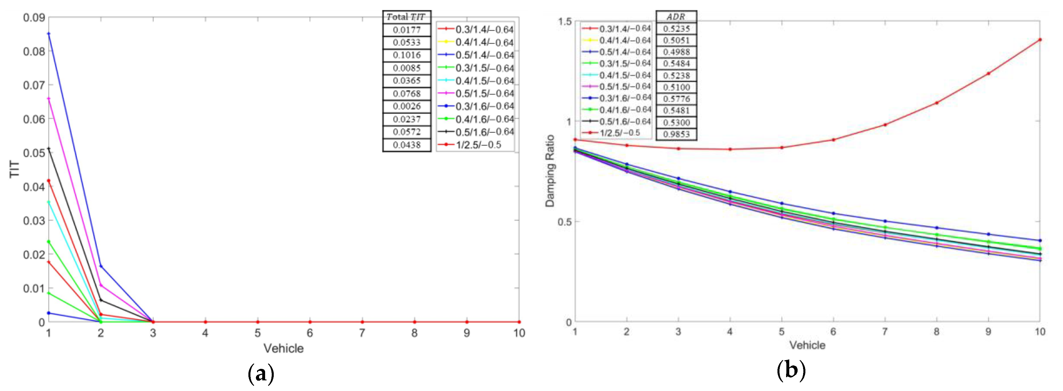
Feedback gains for the CAV (AV) controller should be carefully designed within a rational range because improper selection of the feedback gains can cause inappropriate driving behaviors. According to reference [27], $k_s$ ranges from 0.3 to 0.5, and $k_v$ ranges from 1.4 to 1.6. $k_a$ fluctuates within a certain range however does not have an obvious effect on the results. Therefore, we set $k_s$ as 0.3, 0.4, 0.5, $k_v$ as 1.4, 1.5, 1.6, and $k_a$ as −0.64 for gain impact analysis. Nine combinations were generated. Other than the above, a combination of 1, 2.5, −0.5 for $k_s$, $k_v$, and $k_a$ was also included for comparison.

In addition, stability can be categorized into local stability and string stability. It is worth noting that local stability is necessary for CAV (AV) controller because it should be always ensured in real driving process. Hence, the feedback gain value candidates of the platoon should primarily check the conditions that have been proved by [29] for local stability. On the other hand, disturbance (e.g., proceeding vehicle acceleration/deceleration) can be the main reason of system string instability and by the process of a rear-end crash, string stability describes how the disturbances are attenuated through vehicle string. The string stability is usually measured by a norm function; we used the disturbance energy norm, i.e., $l_2$-norm to measure string stability and to give insights in safety performance. Note that $\Vert a_i{\left(t\right)\Vert }_{l_2}$ denotes $l_2$-norm of $a_i\left(t\right)$, which can be approximated by the Riemann sum. According to reference [27], the sufficient and necessary condition for a CAV system to be string stable is $\Vert a_i{\left(t\right)\Vert }_{l_2}\le \Vert a_{i-1}{\left(t\right)\Vert }_{l_2}$. Moreover, to quantify the disturbance attenuation and better interpret the development trend of platoon’s string stability performance, we defined the damping ratio ($D{R}_i$) for each following vehicle $i$ and platoon average damping ratio (ADR) as below:

$$D{R}_i=\frac{{{\displaystyle \sum }}_{t=1}^T\Vert a_i{\left(t\right)\Vert }_{l_2} }{{{\displaystyle \sum }}_{t=1}^T\Vert a_l{\left(t\right)\Vert }_{l_2} }$$

(14)

$$ADR=\sqrt[N]{{{\displaystyle \prod }}_{i=1}^{N}D{R}_i}$$

(15)

where $a_l$ denotes the acceleration of the leading vehicle, $a_i$ is the acceleration of the following vehicle i, ${\displaystyle \prod }_{i=1}^{N}D{R}_i$ means the product of damping ratio sequence, and $\sqrt[N]{·}$ represents the Nth root.

To analyze the performance for each individual vehicle microscopically, and meanwhile show the trend of TIT through vehicle string, our experiment was implemented on a platoon consisting of 10 CAV followers whose initial states were at the equilibrium point (0,0,0). To eliminate the specialty of a single trajectory that may cause bias in conclusion, the trajectory of the leading vehicle applied the data from a randomly generated dataset including 20 trajectories. The simulation ran for 20 different trials and then the average value was taken. The sampling period was every one-tenth of a second and the total experiment time duration was 45 s, which is usually sufficient to cover a whole ‘stop and go’ for a single vehicle during a traffic oscillation. Note that because the CAVs usually have better capability to conduct car following tasks, we enhanced the default TTC threshold to 5 s to better show the trend of TIT through vehicle strings. A sensitivity analysis on the TTC threshold value is given in a later section. Furthermore, to circumvent over-aggressiveness and over-conservativeness, the controller’s default desired time headway was selected to be 1.2 s. We calculated the platoon’s TIT value and damping ratio under ten different combinations of feedback gains, respectively. The results are shown in Figure 3.

In Figure 3a, it can be seen that some feedback gain combinations have zero-value TIT from the second vehicle whilst others are from the third vehicle, showing the different beginning locations of being totally safe in the platoon. The results imply that SSMs and string stability generally follows a correlative relationship. Besides, we also plot the platoon damping ratio in Figure 3b, in which all candidate combinations except for the comparison are string stable for the monotonous decreasing trend. When the platoon is string stable, the magnitudes of $k_s$ and $k_v$ can determine different performances of platoon. Specifically, we found that smaller $k_s$ and larger $k_v$ (0.3/1.6/−0.64) performs better in terms of platoon TIT, whereas, larger $k_s$ and smaller $k_v$ (0.5/1.4/−0.64) tended to have better performance with respect to damping ratio. The potential reason for this phenomenon could be a larger setting on $k_s$ which may lead the controller to overacting on velocity difference. On the contrary, when $k_v$ is relatively large, the speeds of two vehicles tend to be consistent, such that TTC value becomes infinity, inferring an absolute safe state.

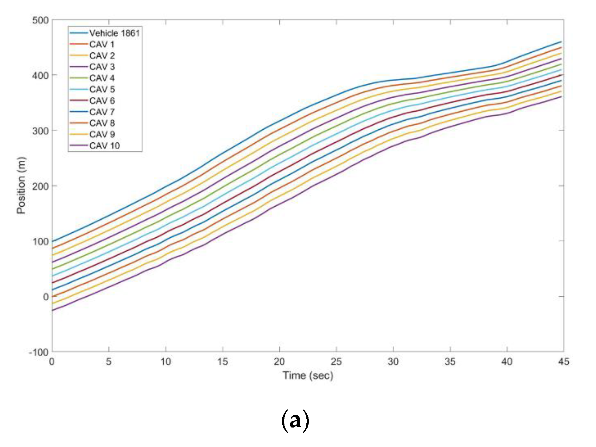
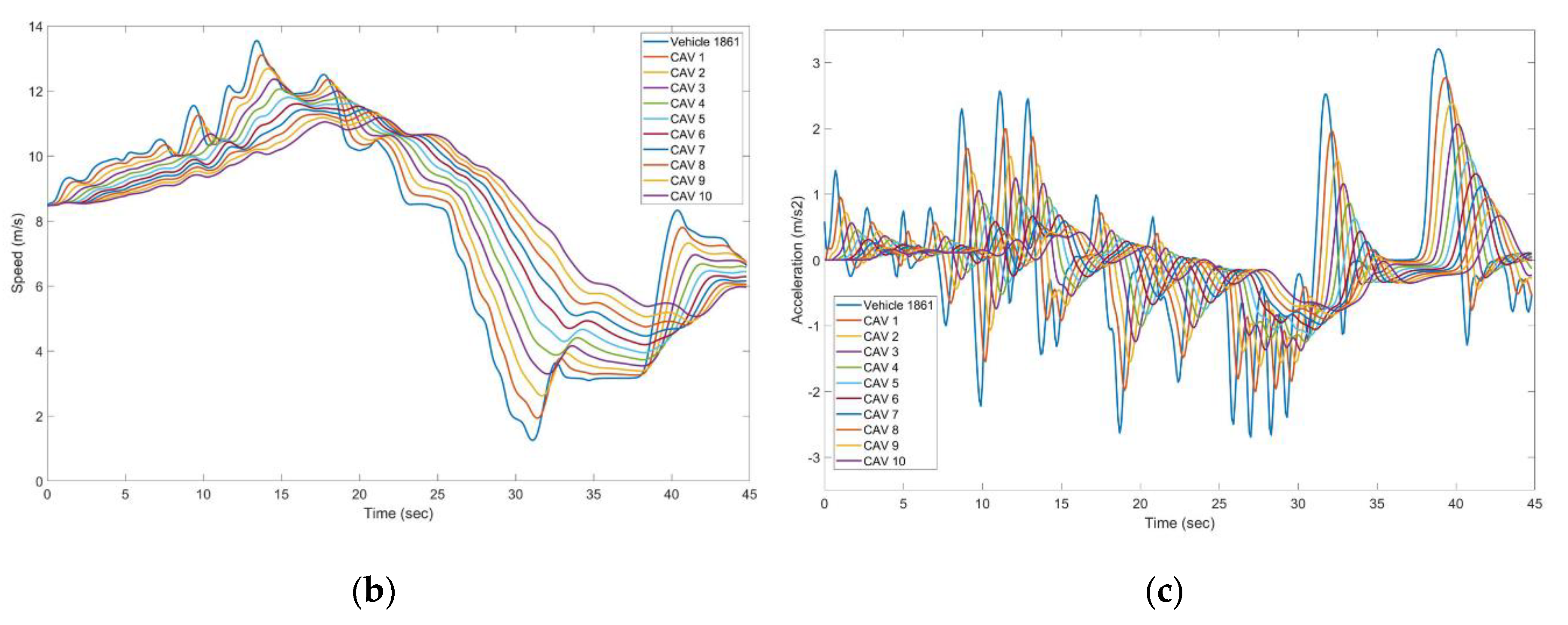
Without loss of generality, we chose the combination of 0.3/1.5/−0.64 for CAV and AV in the following experiments. As an example, Figure 4 plots the trajectory information used to compute SSMs and stability measures with the selected feedback gains. The leading HDV of the platoon is numbered 1861 whose driving data were extracted from the NGSIM database [30]. A proper filter has been applied on origin trajectory data to acquire clean data without sudden acceleration change or other wrong information.

2.

CAV controller communication delay

In this subpart, a pure CAV platoon with 15 followers were established. According to reference [31], communication delay is usually assumed to be 0.2 s or 0.4 s for the CAV controller. As a comparison, the controller without any delay was also studied as an ideal case, due to the increasing maturity of 5G and even 6G technology. Furthermore, TTC threshold values normally range from 1 s to 4 s based on some previous references, e.g., reference [18]. It is worth noting that for a more insightful analysis and strict safety requirement, the critical threshold was extended up to 5 s in this paper. $t^{*}$ was set as 1.2 s. The leading vehicle’s trajectory was also applied from the aforementioned 20-trajectory dataset. The results are shown in

Table 2. CACC communication delay impact analysis.

Communication Delay	$\mathit{\theta }=0 \mathbf{s}$	$\mathit{\theta }=0.2 \mathbf{s}$	$\mathit{\theta }=0.4 \mathbf{s}$
$TT{C}^{*}=1 \mathrm{s}$	0	0	0
$TT{C}^{*}=2 \mathrm{s}$	0	0	0.0006
$TT{C}^{*}=3 \mathrm{s}$	0	0.0016	0.0089
$TT{C}^{*}=4 \mathrm{s}$	0.0006	0.0068	0.0285
$TT{C}^{*}=5 \mathrm{s}$	0.0032	0.0159	0.0852
ADR	0.4649	0.5484	0.7598
Stable	Yes	Yes	Yes

.

A negative effect on TIT is shown as communication delay increases. The main reason can be derived from larger communication delays resulting in more acceleration information lag such that the information may be outdated. Besides, we found that further increment of communication delay can lead to string instability and extremely large TIT values. This part is omitted due to the limited space. We set $\theta =0.2 \mathrm{s}$ for the following experiments.

4.1.2. Equilibrium Condition

The desired (equilibrium) time headway affects the controller’s convergent speed to the equilibrium point which also has a close relationship with driving behavior. According to reference [31], desired time headway’s setting considers 1 s, 1.2 s, 1.5 s. The results are provided in

Table 3. CACC equilibrium time gap impact analysis

${\mathit{t}}^{*}$	$1 \mathbf{s}$	$1.2 \mathbf{s}$	$1.5 \mathbf{s}$
$TT{C}^{*}=1 \mathrm{s}$	0	0	0
$TT{C}^{*}=2 \mathrm{s}$	0	0	0
$TT{C}^{*}=3 \mathrm{s}$	0.0030	0.0016	0.0011
$TT{C}^{*}=4 \mathrm{s}$	0.0118	0.0068	0.0038
$TT{C}^{*}=5 \mathrm{s}$	0.0360	0.0159	0.0085
ADR	0.6046	0.5484	0.4776
Stable	Yes	Yes	Yes

. From Table 3, the conclusion can be drawn that performances of TIT become better as desired time headway grows. Obviously, larger desired time headway setting guarantees system safety better due to a larger equilibrium spacing under constant time headway (CTH) policy, however, it can simultaneously worsen car-following performance of vehicular system and reduce throughput. Therefore, by judging the trade-off between rear-end crash risk and system performance, controller’s desired time headway should choose 1.2 s. Moreover, the TIT value improves as TTC threshold increases due to an increased dangerous duration included and the increased part $\frac{1}{TTC\left(t\right)}-\frac{1}{TT{C}^{*}}$ in TIT computing.

4.2. Macroscopic Parametric Impact Analysis

Macroscopic parameters focus on platoon-level characteristics. CAV MPR and vehicle topology are two vital parameters in platoon trajectory generation, which could further influence platoon safety. In addition, to avoid negative impacts owing to the degradation, platoon’s SSM under V2V environment were also analyzed as a comparison.

4.2.1. CAV Market Penetration Rate

Different MPRs of CAVs in the mixed platoon have essential influences on SSMs. In this subpart, CAVs were introduced to the platoon with a 20% increment. We simulated a pure HDV platoon, mixed platoons with 20%, 40%, 60%, 80% MPR of CAV, and a purely CAV platoon, respectively. All the aforementioned strings have 10 following vehicles. The trajectories of the leading vehicle were also obtained from the dataset. Set $TT{C}^{*}=5 \mathrm{s}$ based on the analysis before. Without loss of generality, several typical vehicle orders were selected for the above CAV MPR circumstances. Moreover, the dangerous probability derived from TET is defined as:

$$p\left(\mathrm{dangerous}\right)=\frac{TE{T}_i}{T\times \Delta \left(t\right)}$$

(16)

where $p\left(\mathrm{dangerous}\right)$ interprets the dangerous degree of each vehicle during total period.

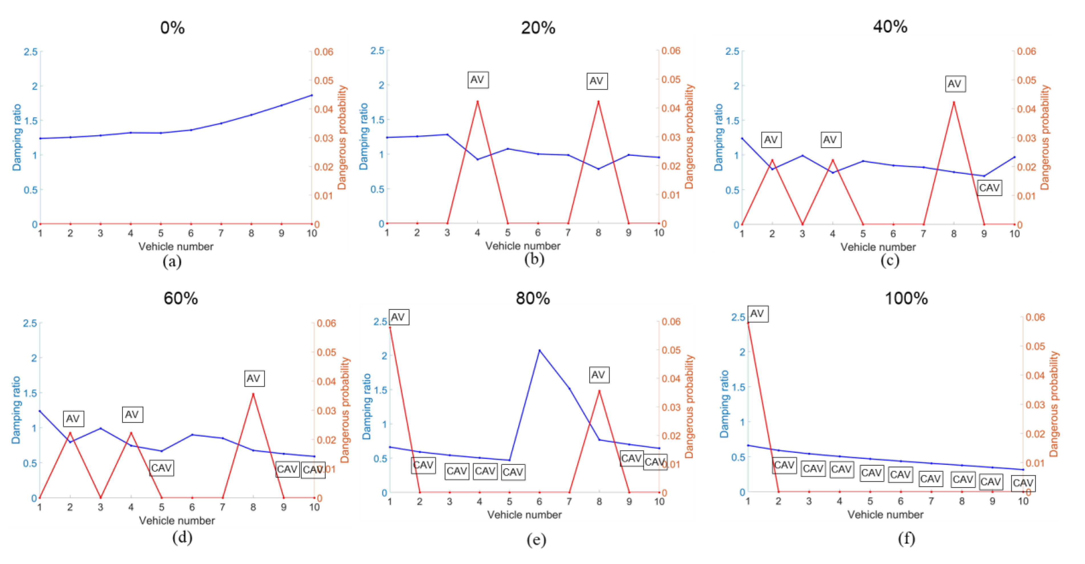
The simulation results considering degradation are shown in

Table 4. Dangerous probability and damping ratio per vehicle under different CAV MPRs.

Dangerous Probability							Damping Ratio
CAV MPR	0%	20%	40%	60%	80%	100%	0%	20%	40%	60%	80%	100%
V1	0.0497	0.0497	0.0497	0.0497	0.1002 1	0.1002	1.1206	1.1026	1.1026	1.1026	0.7801	0.7801
V2	0.0421	0.0421	0.1072	0.1072	0.0000	0.0000	1.1271	1.1271	0.7327	0.7273	0.6384	0.6384
V3	0.0446	0.0446	0.0283	0.083	0.0000	0.0000	1.1281	1.1281	0.9306	0.9306	0.5747	0.5474
V4	0.0446	0.1172	0.0876	0.0876	0.0000	0.0000	1.1714	0.8048	0.6422	0.6422	0.5179	0.5179
V5	0.0519	0.0452	0.0240	0.0000	0.0000	0.0000	1.2356	1.0493	0.8716	0.5848	0.4674	0.4674
V6	0.0604	0.0472	0.0281	0.0249	0.0193	0.0000	1.2956	1.1115	0.9027	0.8627	0.8365	0.4230
V7	0.0713	0.0510	0.0319	0.0260	0.0186	0.0000	1.3478	1.1746	0.9439	0.8990	0.8609	0.3844
V8	0.0790	0.1251	0.0998	0.0808	0.0590	0.0000	1.3917	0.7928	0.7069	0.6464	0.6352	0.3511
V9	0.0852	0.0536	0.0000	0.0000	0.0000	0.0000	1.3906	1.0296	0.6607	0.5974	0.5818	0.3222
V10	0.0868	0.0548	0.0398	0.0000	0.0000	0.0000	1.3845	1.0901	0.9360	0.5539	0.5336	0.2968
AVE	0.0616	0.0630	0.0496	0.0404	0.0197	0.0100	1.1183	1.0161	0.9108	0.8581	0.7900	0.6712

¹ Bold numbers in table means a CAV or AV.

. From the results, both dangerous probability and damping ratio in a purely HDV platoon (0%) have an overall amplified trend through the string, indicating the unsafety and instability property for HDVs. Focusing on the dangerous probability, we have similar conclusions with reference [18]. Notice that when CAV MPR is less than 20%, the mixed platoon’s safety performance is even worse compared with a full HDV platoon. The reason can be derived from CAVs having a large likelihood to degrade to AV under low CAV MPR, and AVs do not have the feedforward term while still maintaining a relatively small headway. Furthermore, a small MPR may introduce heterogeneities to traffic flow, which may also cause some car following safety issues. Nevertheless, when CAV MPR exceeds 20%, the dangerous probability will decay gradually as the MPR increases. This is achieved because CAVs in the platoon can improve the whole platoon’s performance due to their own outstanding safety performances (See MPR 40%, V9, MPR 80%, V2). Moreover, we also investigated the string stability performances in terms of damping ratio to evaluate the influence of CAVs (AVs) on oscillation dissipation. Results show that with the increment of CAV MPR, the damping ratio of a vehicle decreases drastically when the original HDV is replaced with an AV (e.g., see MPR = 20%, V4) while there is a slower decline from AV to CAV (e.g., see MPR = 40%, V9). An HDV after an AV or CAV increases the damping ratio again. This phenomenon validates that the feedback mechanism embedded in CAV/AV controller has a stronger ability to ameliorate oscillation compared with the feedforward mechanism. Although the string stability has been improved by CAV when MPR is 20%, string stability is just one of the factors affecting car following safety. One key reason is that the string stability only guarantees the acceleration attenuation. The over acceleration smoothness may contribute to the speed difference and cause some potential car following safety risk. The heterogeneity caused by CAV degradation can also be another potential reason. In general, SSMs and string stability measures have a qualitative relationship with respect to CAV MPR.

As an example, and to be more intuitive, $p\left(\mathrm{dangerous}\right)$ per vehicle and damping ratio of a platoon led by vehicle number 1861 from NGSIM database are illustrate in Figure 5, in which vehicle orders in platoon are also elucidated. Vehicles without other notations in the following figures are HDV.

4.2.2. Vehicle Topology

Except for the CAV proportion in the platoon, the vehicle topology formation is then studied under identical CAV MPR for a more in-depth analysis. Without loss of generality, a 50% CAV MPR was chosen. In practice, there are usually four kinds of car following modes, including: (1) vehicles in the former part are CAVs and the following part are HDVs, called “CAV first” (CCCCCHHHHH); (2) vehicles in the former part are HDVs and the following part are CAVs, called “HDV first” (HHHHHCCCCC); (3) HDVs and CAVs are arranged alternately (CHCHCHCHCH); (4) randomly ordered (e.g., CHHCHCHCCC).

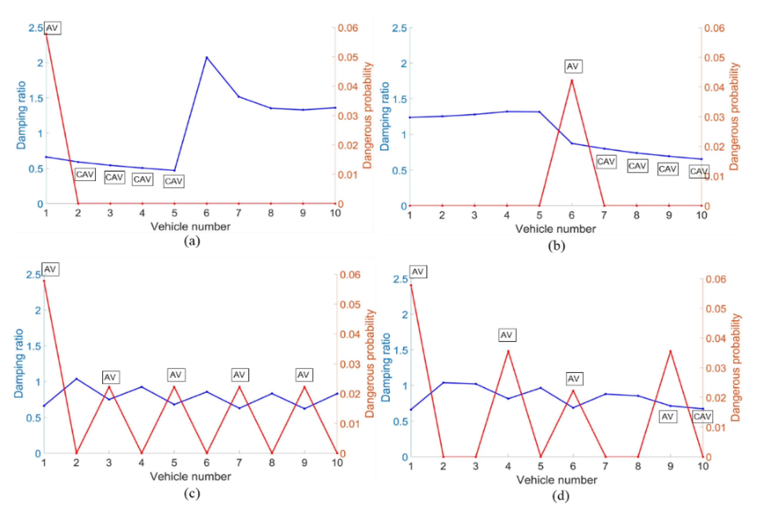
Simulation results are presented in

Table 5. Platoon damping ratio and dangerous probability under 50% MPR

${\mathit{t}}^{*}$	Dangerous Probability	Average Damping Ratio
Situation 1	0.0200	0.8451
Situation 2	0.0389	0.9483
Situation 3	0.0549	0.8542
Situation 4	0.0453	0.8895

using the trajectory dataset mentioned above. Results show that situation 1 has best performance for both dangerous probability and average damping ratio. In situation 1, disturbance from the leading vehicle has been adjusted by the front CAVs of the mixed platoon such that oscillation will not be amplified through the propagation to the back HDVs, thus the platoon becomes safer. Situation 4 takes the average values of all random orders in Dangerous probability and Average damping ratio except the orders in Situation 1, 2 and 3. Results show that Situation 4 performs between situation 2 and situation 3 from both perspectives. Hence, under the same CAV MPR, we should set CAVs at the front as much as possible to achieve a better performance. Correspondingly, Figure 6 plots the aforementioned four situations with vehicle 1861 as the leading vehicle. Situation 4 illustrated here is a characteristic case of random order.

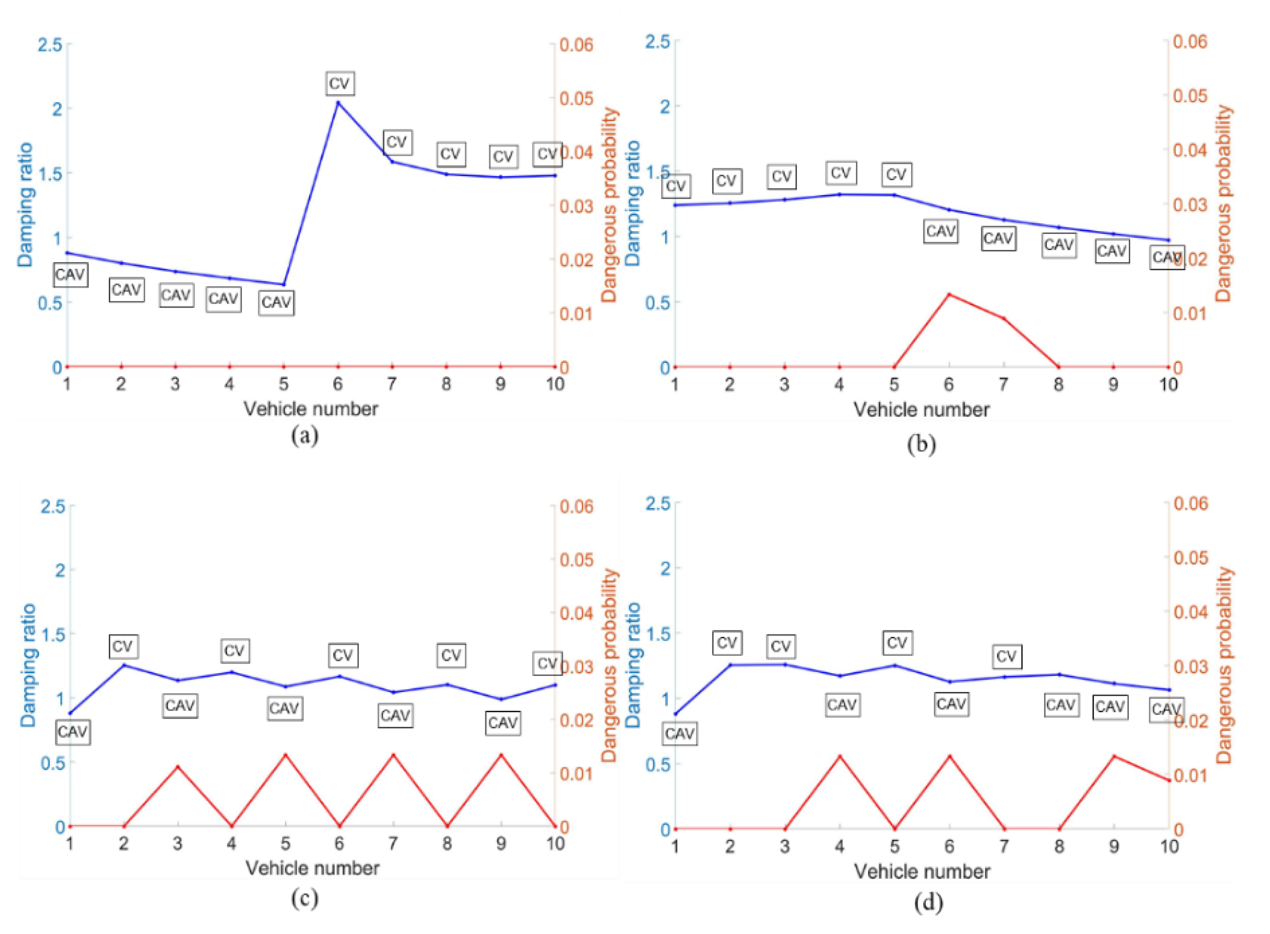
4.3. V2V Environment

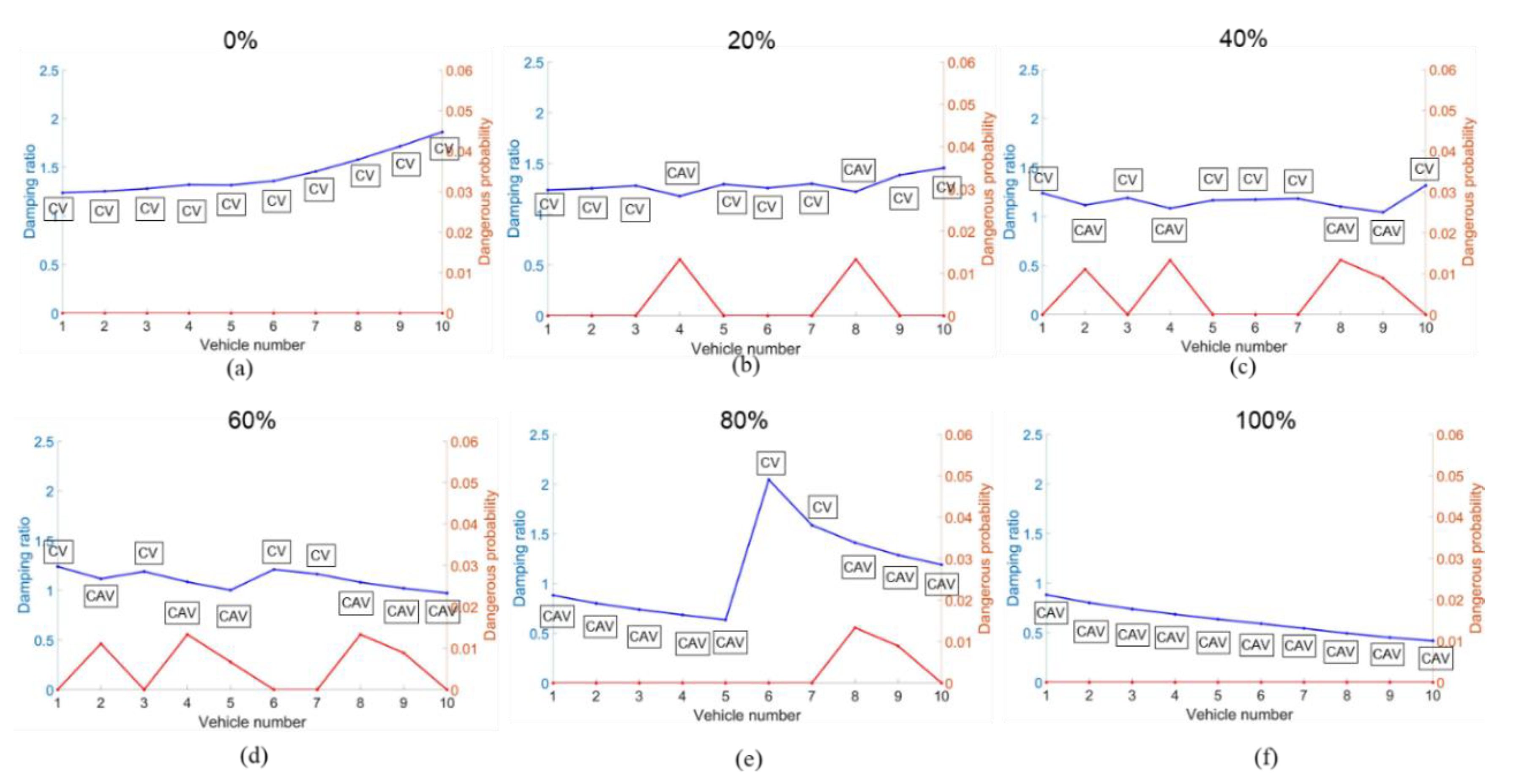
From the previous experiments, we can acknowledge that degradation of CAV can locally weaken the improvement of SSMs in the mixed platoon. Hence, to compensate for degradation, we considered building a V2V environment in which a communication device is added to every HDV. HDV then upgrades to a connected vehicle (CV) because it can transfer its current driving state to the follower. Under this circumstance, no communication degradation will occur. We evaluate the identical situations set for CAV MPR and vehicle topology in the former part.

Table 6. Dangerous probability and damping ratio per vehicle under different CAV MPRs in a V2V environment.

Dangerous Probability							Damping Ratio
CAV MPR	0%	20%	40%	60%	80%	100%	0%	20%	40%	60%	80%	100%
V1	0.0497	0.0497	0.0497	0.0497	0.0060 1	0.0060	0.0060	0.0666	0.0060	0.0060	0.0497	0.0497
V2	0.0421	0.0421	0.0179	0.0179	0.0018	0.0018	0.0018	0.0488	0.0492	0.0492	0.0421	0.0421
V3	0.0446	0.0446	0.0364	0.0364	0.0010	0.0010	0.0010	0.0429	0.0164	0.0368	0.0446	0.0446
V4	0.0446	0.0271	0.0189	0.0189	0.0002	0.0002	0.0002	0.0440	0.0338	0.0222	0.0446	0.0271
V5	0.0519	0.0542	0.0310	0.0182	0.0000	0.0000	0.0000	0.0531	0.0181	0.0416	0.0519	0.0542
V6	0.0604	0.0601	0.0321	0.0349	0.0190	0.0000	0.0174	0.0319	0.0274	0.0260	0.0604	0.0601
V7	0.0713	0.0689	0.0426	0.0438	0.0236	0.0000	0.0223	0.0309	0.0197	0.0364	0.0713	0.0689
V8	0.0790	0.0427	0.0287	0.0346	0.0210	0.0000	0.0270	0.0280	0.0273	0.0403	0.0790	0.0427
V9	0.0852	0.0883	0.0278	0.0307	0.0211	0.0000	0.0332	0.0228	0.0208	0.0287	0.0852	0.0883
V10	0.0868	0.0956	0.0569	0.0246	0.0186	0.0000	0.0404	0.0717	0.0331	0.0274	0.0868	0.0956
Mean	0.0616	0.0573	0.0342	0.0310	0.0112	0.0009	0.0149	0.0386	0.0252	0.0315	0.0616	0.0573

¹ Bold numbers in table mean a CAV or AV.

shows the results.

With the mixed platoon cases with degradation tested before set as benchmarks, we observed that the SSM-related performances were all improved. This can be attributed to the additional feedforward term setting on CAV controllers that more comprehensive information can be provide through V2V process compared with AV. Besides, with the pure CV platoon set as a benchmark, the dangerous probability starts to decay immediately when CAVs are introduced to the platoon, inferring the CV’s effectiveness of safety improvement on probability declining. This also explains the significance of feedforward control. For vehicle topology, situation 1 is still the best choice. Similarly, Figure 7 and Figure 8 illustrate performances corresponding to the situations in V2V environment with 1861 as leading vehicle.

5. Conclusions and Discussion

This paper conducted a systematically parametric impact analysis on SSM for a mixed platoon consisting of CAV, AV, and HDV via a proposed two-level active safety evaluation framework. By performing simulation experiments, we found that for a single vehicle, the higher order dynamics of CAVs affected by equilibrium time gap, feedback and feedforward mechanism. CAV serve as the major factor to ensure SSM performance. The results imply that SSM and string stability generally follows a correlative relationship, and larger speed difference feedback gains over the string stability region can further help to enhance the car-following safety. Furthermore, we also figured out that communication degradation of CAVs can be a potential unsafe component. For the whole platoon, the platoon safety performance in terms of SSMs can be improved only after they exceed a certain level of CAV MPR considering degradation. Furthermore, rather than simply analyzing the MPR impact, we further analyzed the vehicle topology impacts on SSM. The findings also suggested that all CAVs should be arranged as close to the front of the mixed platoon as possible to achieve a better SSM performance from a vehicle topology perspective. As a remedy, we found that upgrading HDVs to CVs can also eliminate negative effects caused by degradation and improve SSM performance to a great extent.

Experimental results conducted in this paper can have some insight meanings for the practical management under partial connected automated environments for sustainability concerns. Firstly, guaranteeing string stability for CAV control is very important to enhance car-following safety, and a proper tuning of controller’s gains and equilibrium spacing can also be one of the most achievable and cost effective ways to enhance car-following safety. Secondly, with the development of communication technology, the communication delay is likely to be reduced, which can facilitate increased car-following safety. We should also manage to reduce CAV degradation happening through changing the vehicle topology formations, such as establishing CAV dedicated lanes, because AVs are the main reason for amplified danger probabilities. Furthermore, adding a V2V communication unit to an HDV is another useful strategy to improve SSMs. However, the process of complete HDV upgrading for device installment is time-consuming, therefore some graceful degradation measures are recommended as a remedy strategy.

6. Limitations and Future Works

Although our paper systematically analyzed the parametric impacts for mixed traffic, there is still some room to further conduct safety analyses: (1). This paper merely took the longitudinal motion into consideration, while the lateral motions such as lane-changing and merging maneuvers were not considered in this research; (2). This paper just applied a decentralized communication topology, while other types of communication topology could be further explored using our framework; (3). The vehicle dynamics and communication delay were treated as nominal values, although in reality they could be time varying and uncertain. Those parts will be further investigated in the future.

References

- Lee, S.E.; Llaneras, E.; Klauer, S.; Sudweeks, J. Analyses of rear-end crashes and near-crashes in the 100-car naturalistic driving study to support rear-signaling countermeasure development. DOT HS 2007, 810, 846. [Google Scholar]
- Ye, L.; Yamamoto, T. Modeling connected and autonomous vehicles in heterogeneous traffic flow. Phys. A Stat. Mech. Its Appl. 2018, 490, 269–277. [Google Scholar] [CrossRef]
- Zheng, Z.; Ahn, S.; Chen, D.; Laval, J. Applications of wavelet transform for analysis of freeway traffic: Bottlenecks, transient traffic, and traffic oscillations. Transp. Res. Part B Methodol. 2011, 45, 372–384. [Google Scholar] [CrossRef] [Green Version]
- Turoń, K.; Kubik, A. Economic aspects of driving various types of vehicles in intelligent urban transport systems, including car-sharing services and autonomous vehicles. Appl. Sci. 2020, 10, 5580. [Google Scholar] [CrossRef]
- Wang, C.; Gong, S.; Zhou, A.; Li, T.; Peeta, S. Cooperative adaptive cruise control for connected autonomous vehicles by factoring communication-related constraints. Transp. Res. Part C Emerg. Technol. 2019, 1–22. [Google Scholar] [CrossRef] [Green Version]
- Ploeg, J.; Semsar-Kazerooni, E.; Lijster, G.; Van De Wouw, N.; Nijmeijer, H. Graceful degradation of CACC performance subject to unreliable wireless communication. IEEE Conf. Intell. Transp. Syst. Proc. ITSC 2013, 1210–1216. [Google Scholar] [CrossRef]
- Nagai, M. The perspectives of research for enhancing active safety based on advanced control technology. User Model. User-Adapt. Interact. 2007, 45, 413–431. [Google Scholar] [CrossRef]
- Hauer, E. Statistical road safety modeling. Transp. Res. Rec. 2004, 1897, 81–87. [Google Scholar] [CrossRef]
- Miaou, S.-P. The relationship between truck accidents and geometric design of road sections: Poisson versus negative binomial regressions. Accid. Anal. Prev. 1994, 26, 471–482. [Google Scholar] [CrossRef] [Green Version]
- Lee, J.; Nam, B.; Abdel-Aty, M. Effects of pavement surface conditions on traffic crash severity. J. Transp. Eng. 2015, 141, 4015020. [Google Scholar] [CrossRef]
- Wu, Y.; Abdel-aty, M.; Cai, Q.; Lee, J.; Park, J. Developing an algorithm to assess the rear-end collision risk under fog conditions using real-time data. Transp. Res. Part C 2018, 87, 11–25. [Google Scholar] [CrossRef]
- Xu, C.; Liu, P.; Yang, B.; Wang, W. Real-time estimation of secondary crash likelihood on freeways using high-resolution loop detector data. Transp. Res. Part C 2016, 71, 406–418. [Google Scholar] [CrossRef]
- Tian, D.; Wu, G. Performance Measurement Evaluation Framework Analysis for Connected and Automated Vehicles (CAV) Applications: A Survey. IEEE Intell. Transp. Syst. Mag. 2018, 10, 110–122. [Google Scholar] [CrossRef] [Green Version]
- Lord, D.; Persaud, B.N. Accident prediction models with and without trend: Application of the generalized estimating equations procedure. Transp. Res. Rec. 2000, 1717, 102–108. [Google Scholar] [CrossRef]
- Li, Y.; Xing, L.; Wang, W.; Wang, H.; Dong, C.; Liu, S. Evaluating impacts of different longitudinal driver assistance systems on reducing multi-vehicle rear-end crashes during small-scale inclement weather. Accid. Anal. Prev. 2017, 107, 63–76. [Google Scholar] [CrossRef]
- Kuang, Y.; Yu, Y.; Qu, X. Novel Crash Surrogate Measure for Freeways. J. Transp. Eng. Part A Syst. 2020, 146, 04020085. [Google Scholar] [CrossRef]
- Meng, Q.; Qu, X. Estimation of rear-end vehicle crash frequencies in urban road tunnels. Accid. Anal. Prev. 2012, 48, 254–263. [Google Scholar] [CrossRef] [Green Version]
- Qin, Y.; Wang, H. Influence of the feedback links of connected and automated vehicle on rear-end collision risks with vehicle-to-vehicle communication. Traffic Inj. Prev. 2019, 20, 79–83. [Google Scholar] [CrossRef]
- Qu, X.; Yang, Y.; Liu, Z.; Jin, S.; Weng, J. Potential crash risks of expressway on-ramps and off-ramps: A case study in Beijing, China. Saf. Sci. 2014, 70, 58–62. [Google Scholar] [CrossRef] [Green Version]
- Xing, L.; He, J.; Abdel-Aty, M.; Cai, Q.; Li, Y.; Zheng, O. Examining traffic conflicts of up stream toll plaza area using vehicles’ trajectory data. Accid. Anal. Prev. 2019, 125, 174–187. [Google Scholar] [CrossRef]
- Li, Y.; Xu, C.; Xing, L.; Wang, W. Integrated Cooperative Adaptive Cruise and Variable Speed Limit Controls for Reducing Rear-End Collision Risks Near Freeway Bottlenecks Based on Micro-Simulations. IEEE Trans. Intell. Transp. Syst. 2017, 18, 3157–3167. [Google Scholar] [CrossRef]
- Rahman, M.S.; Abdel-Aty, M.; Lee, J.; Rahman, M.H. Safety benefits of arterials’ crash risk under connected and automated vehicles. Transp. Res. Part C Emerg. Technol. 2019, 100, 354–371. [Google Scholar] [CrossRef]
- Virdi, N.; Grzybowska, H.; Waller, S.T.; Dixit, V. A safety assessment of mixed fleets with Connected and Autonomous Vehicles using the Surrogate Safety Assessment Module. Accid. Anal. Prev. 2019, 131, 95–111. [Google Scholar] [CrossRef]
- Qin, Y.Y.; He, Z.Y.; Ran, B. Rear-end crash risk of CACC-Manual driven mixed flow considering the degeneration of CACC systems. IEEE Access 2019, 7, 140421–140429. [Google Scholar] [CrossRef]
- Bando, M.; Hasebe, K.; Nakanishi, K.; Nakayama, A. Analysis of optimal velocity model with explicit delay. Phys. Rev. E-Stat. Physics, Plasmas, Fluids, Relat. Interdiscip. Top. 1998, 58, 5429–5435. [Google Scholar] [CrossRef] [Green Version]
- Koshi, M. Some findings and an overview on vehicular flow characteristics. In Proceedings of the Eighth International Symposium on Transportation and Traffic Theory, Toronto, ON, Canada, 24–26 June 1981. [Google Scholar]
- Zhou, Y.; Ahn, S.; Wang, M.; Hoogendoorn, S. Stabilizing mixed vehicular platoons with connected automated vehicles: An H-infinity approach. Transp. Res. Part B Methodol. 2020, 132, 152–170. [Google Scholar] [CrossRef]
- Minderhoud, M.M.; Bovy, P.H.L. Extended time-to-collision measures for road traffic safety assessment. Accid. Anal. Prev. 2001, 33, 89–97. [Google Scholar] [CrossRef]
- Zhou, Y.; Wang, M.; Ahn, S. Distributed model predictive control approach for cooperative car-following with guaranteed local and string stability. Transp. Res. Part B Methodol. 2019, 128, 69–86. [Google Scholar] [CrossRef]
- Ge, J.I.; Avedisov, S.S.; He, C.R.; Qin, W.B.; Sadeghpour, M.; Orosz, G. Experimental validation of connected automated vehicle design among human-driven vehicles. Transp. Res. Part C Emerg. Technol. 2018, 91, 335–352. [Google Scholar] [CrossRef]
- Punzo, V.; Teresa, M.; Ciuffo, B. On the assessment of vehicle trajectory data accuracy and application to the Next Generation SIMulation (NGSIM) program data. Transp. Res. Part C. 2011, 19, 1243–1262. [Google Scholar] [CrossRef]
Figure 1.
Flowchart of the two-level active safety evaluation.
Figure 2.
Schematic diagram of mixed platoon car-following relationship.
Figure 3.
Parameter impact analysis on controller feedback gains: (a) TIT for each vehicle; (b) Damping ratio for each vehicle.
Figure 4.
Trajectory of example case system: (a) Position; (b) Speed; (c) Acceleration.
Figure 5.
Damping ratio and dangerous probability per vehicle of example case under different CAV (AV) market penetration rate considering degradation: (a) 0%; (b) 20%; (c) 40%; (d) 60%; (e) 80%; (f) 100%.
Figure 6.
Mixed vehicle system dangerous probability and damping ratio under 50% CAV(AV) market penetration: (a) Situation 1; (b) Situation 2; (c) Situation 3; (d) Situation 4.
Figure 7.
Damping ratio and dangerous probability per vehicle of example case under different CAV (AV) market penetration rate without degradation: (a) 0%; (b) 20%; (c) 40%; (d) 60%; (e) 80%; (f) 100%.
Figure 8.
Mixed vehicle system dangerous probability and damping ratio under 50% CAV(AV) market penetration in V2V environment: (a) Situation 1; (b) Situation 2; (c) Situation 3; (d) Situation 4.