Predicting the Impact of Climate Change on Freshwater Fish Distribution by Incorporating Water Flow Rate and Quality Variables

 and
and
Abstract
:1. Introduction
2. Data and Methodology
2.1. Study Area and Fish Data
2.2. Environmental Data
2.3. Species Distribution Modeling
3. Results and Discussion
3.1. Model Performance
3.2. Overall Prediction of Fish Distribution
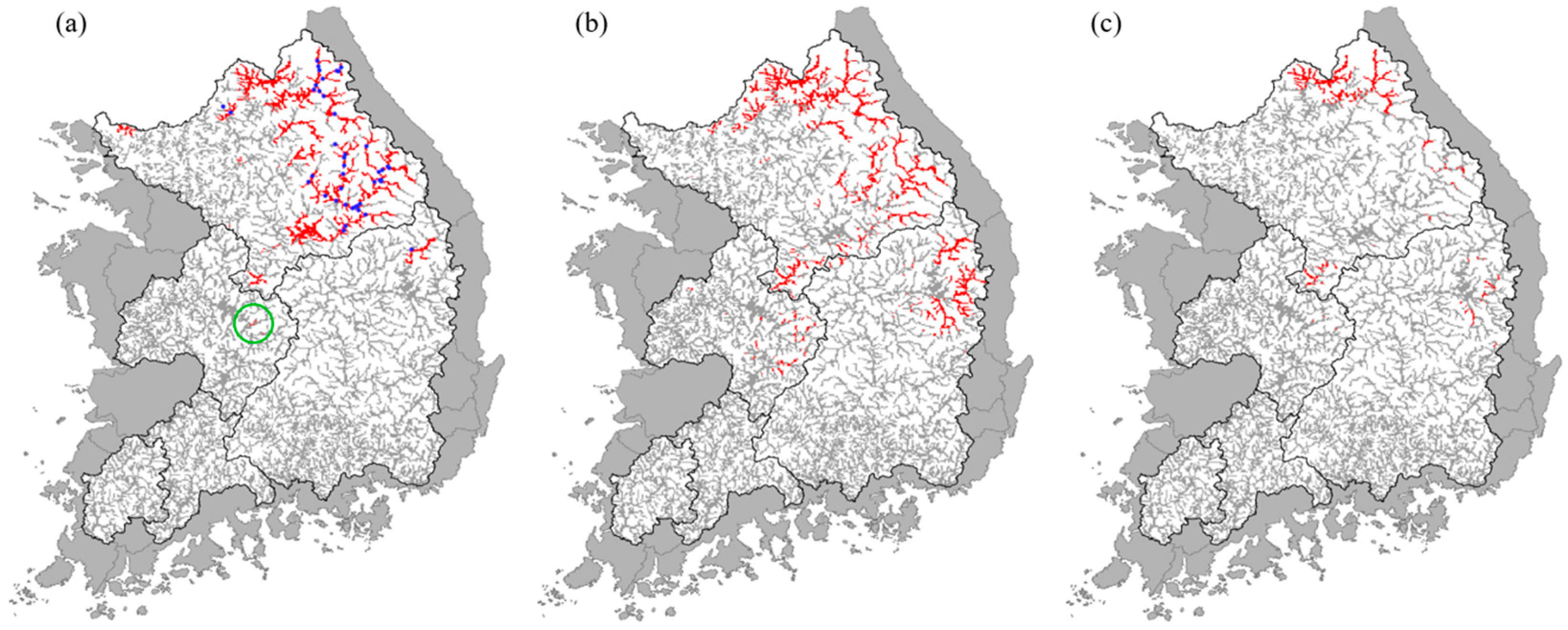
3.3. Predicted Distribution of Korean Spotted Barbel
3.4. Model Limitations and Challenges
4. Conclusions
Supplementary Materials
Author Contributions
Funding
Acknowledgments
Conflicts of Interest
References
- Markovic, D.; Carrizo, S.; Freyhof, J.; Cid, N.; Lengyel, S.; Scholz, M.; Kasperdius, H.; Darwall, W. Europe’s freshwater biodiversity under climate change: Distribution shifts and conservation needs. Divers. Distrib. 2014, 20, 1097–1107. [Google Scholar] [CrossRef]
- Novak, M.; Moore, J.W.; Leidy, R.A. Nestedness patterns and the dual nature of community reassembly in California streams: A multivariate permutation-based approach. Glob. Chang. Biol. 2011, 17, 3714–3723. [Google Scholar] [CrossRef]
- IPCC (Intergovernmental Panel on Climate Change). Climate Change 2013: The Physical Science Basis. Contribution of Working Group I to the Fifth Assessment Report of the Intergovernmental Panel on Climate Change; Stocker, T.F., Qin, D., Plattner, G.K., Tignor, M., Allen, S.K., Boschung, J., Nauels, A., Xia, Y., Bex, V., Midgley, P.M., Eds.; Cambridge University Press: Cambridge, UK; New York, NY, USA, 2013. [Google Scholar]
- NIMR. Korean Peninsula Climate Change Outlook Report; Publication Number: 11-1360000-000861-01; NIMR: Seoul, Korea, 2011.
- Koo, K.A.; Kong, W.S.; Nibbelink, N.P.; Hopkinson, C.S.; Lee, J.H. Potential Effects of Climate Change on the Distribution of Cold-Tolerant Evergreen Broadleaved Woody Plants in the Korean Peninsula. PLoS ONE 2015, 10, e0134043. [Google Scholar] [CrossRef]
- Lim, C.H.; Yoo, S.; Choi, Y.; Jeon, S.W.; Son, Y.; Lee, W.K. Assessing Climate Change Impact on Forest Habitat Suitability and Diversity in the Korean Peninsula. Forests 2018, 9, 259. [Google Scholar] [CrossRef] [Green Version]
- Kwon, Y.S.; Bae, M.J.; Hwang, S.J.; Kim, S.H.; Park, Y.S. Predicting potential impacts of climate change on freshwater fish in Korea. Ecol. Inform. 2015, 29, 156–165. [Google Scholar] [CrossRef]
- Pandit, S.N.; Maitland, B.M.; Pandit, L.K.; Poesch, M.S.; Enders, E.C. Climate change change risks, extinction debt, and conservation implications for a threatened freshwater fish: Carmine shiner (Notropis percobromus). Sci. Total Environ. 2017, 598, 1–11. [Google Scholar] [CrossRef]
- Friedman, J.H. Multivariate Adaptive Regression Splines. Ann. Stat. 1991, 19, 1–67. [Google Scholar] [CrossRef]
- Cortes, C.; Vapnik, V. Support-Vector Networks. Mach. Learn. 1995, 20, 273–297. [Google Scholar] [CrossRef]
- Elith, J.; Graham, C.H.; Anderson, R.P.; Dudik, M.; Ferrier, S.; Guisan, A.; Hijmans, R.J.; Huettmann, F.; Leathwick, J.R.; Lehmann, A.; et al. Novel methods improve prediction of species’ distributions from occurrence data. Ecography 2006, 29, 129–151. [Google Scholar] [CrossRef] [Green Version]
- Phillips, S.J.; Anderson, R.P.; Schapire, R.E. Maximum entropy modeling of species geographic distributions. Ecol. Model. 2006, 190, 231–259. [Google Scholar] [CrossRef] [Green Version]
- Wisz, M.S.; Hijmans, R.J.; Li, J.; Peterson, A.T.; Graham, C.H.; Guisan, A.; Distribut, N.P.S. Effects of sample size on the performance of species distribution models. Divers. Distrib. 2008, 14, 763–773. [Google Scholar] [CrossRef]
- Poulos, H.M.; Chernoff, B.; Fuller, P.L.; Butman, D. Ensemble forecasting of potential habitat for three invasive fishes. Aquat. Invasions 2012, 7, 59–72. [Google Scholar] [CrossRef]
- Warren, D.L.; Seifert, S.N. Ecological niche modeling in Maxent: The importance of model complexity and the performance of model selection criteria. Ecol. Appl. 2011, 21, 335–342. [Google Scholar] [CrossRef] [Green Version]
- Frederico, R.; Zuanon, J.; De Marco, P. Amazon protected areas and its ability to protect stream-dwelling fish fauna. Biol. Conserv. 2018, 219, 12–19. [Google Scholar] [CrossRef]
- Growns, I.; Rourke, M.; Gilligan, D. Toward river health assessment using species distributional modeling. Ecol. Indic. 2013, 29, 138–144. [Google Scholar] [CrossRef]
- Liang, L.; Fei, S.; Ripy, J.; Blandford, B.; Grossardt, T. Stream habitat modelling for conserving a threatened headwater fish in the upper cumberland river, Kentucky. River Res. Appl. 2013, 29, 1207–1214. [Google Scholar] [CrossRef]
- Guisan, A.; Thuiller, W. Predicting species distribution: Offering more than simple habitat models. Ecol. Lett. 2005, 8, 993–1009. [Google Scholar] [CrossRef]
- Hughes, R.M.; Gammon, J.R. Longitudinal changes in fish assemblages and water quality in the Willamette River, Oregon. Trans. Am. Fish. Soc. 1987, 116, 196–209. [Google Scholar] [CrossRef]
- Reyjol, Y.; Lim, P.; Belaud, A.; Lek, S. Modelling of microhabitat used by fish in natural and regulated flows in the river Garonne (France). Ecol. Model. 2001, 146, 131–142. [Google Scholar] [CrossRef]
- Tsadik, G.G.; Bart, A.N. Effects of feeding, stocking density and water-flow rate on fecundity, spawning frequency and egg quality of Nile tilapia, Oreochromis niloticus (L.). Aquaculture 2007, 272, 380–388. [Google Scholar] [CrossRef]
- Hockley, F.A.; Wilson, C.A.M.E.; Brew, A.; Cable, J. Fish responses to flow velocity and turbulence in relation to size, sex and parasite load. J. R. Soc. Interface 2014, 11. [Google Scholar] [CrossRef] [PubMed] [Green Version]
- Bradie, J.; Leung, B. A quantitative synthesis of the importance of variables used in MaxEnt species distribution models. J. Biogeogr. 2017, 44, 1344–1361. [Google Scholar] [CrossRef]
- Official Site of Water Environment Information System. Available online: http://water.nier.go.kr/ (accessed on 21 February 2017).
- NIER. Survey and Assessment of Stream/River Ecosystem Health (VII); Publication Number: 11-1480523-002181-01; NIER: Incheon, Korea, 2014.
- Official Site of Korea Meteorological Administration. Available online: http://www.climate.go.kr/ (accessed on 24 February 2017).
- Official Site of ESRI. Available online: https://www.esri.com/en-us/home/ (accessed on 16 January 2017).
- Arnold, J.G.; Moriasi, D.N.; Gassman, P.W.; Abbaspour, K.C.; White, M.J.; Srinivasan, R.; Santhi, C.; Harmel, R.D.; van Griensven, A.; Van Liew, M.W.; et al. Swat: Model Use, Calibration, and Validation. Trans. ASABE 2012, 55, 1491–1508. [Google Scholar] [CrossRef]
- Engel, B.; Storm, D.; White, M.; Arnold, J.; Arabi, M. A Hydrologic/Water Quality Model Application Protocol. J. Am. Water Resour. Assoc. 2007, 43, 1223–1236. [Google Scholar] [CrossRef]
- Official Site of Water Resources Management Information System. Available online: http://www.wamis.go.kr/ (accessed on 21 February 2017).
- Douglas-Mankin, K.R.; Srinivasan, R.; Arnold, J.G. Soil and Water Assessment Tool (Swat) Model: Current Developments and Applications. Trans. ASABE 2010, 53, 1423–1431. [Google Scholar] [CrossRef]
- Neitsch, S.L.; Arnold, J.G.; Kiniry, J.R.; Williams, J.R. Soil and Water Assessment Tool Theoretical Documentation Version 2009; Texas Water Resources Institute: College Station, TX, USA, 2011. [Google Scholar]
- Official Site of National Geographic Information Institute. Available online: http://www.ngii.go.kr/ (accessed on 6 February 2017).
- Official Site of National Institute of Agricultural Sciences. Available online: http://www.naas.go.kr/ (accessed on 6 February 2017).
- Official Site of Maxent. Available online: https://biodiversityinformatics.amnh.org/open_source/maxent/ (accessed on 15 March 2017).
- Hanley, J.A.; McNeil, B.J. The meaning and use of the area under a receiver operating characteristic (ROC) curve. Radiology 1982, 143, 29–36. [Google Scholar] [CrossRef] [Green Version]
- Klemm, D.J.; Stober, Q.J.; Lazorchak, J.M. Fish Field and Laboratory Methods for Evaluating the Biological Integrity of Surface Waters; US EPA: Cincinnati, OH, USA, 1993.
- NIER. Development of Biological Criteria for Water Quality Assessment Using Aquatic Organisms (II); NIER: Incheon, Korea, 2009.
- Swets, J.A. Measuring the Accuracy of Diagnostic Systems. Science 1988, 240, 1285–1293. [Google Scholar] [CrossRef] [Green Version]
- Lobo, J.M.; Jimenez-Valverde, A.; Real, R. AUC: A misleading measure of the performance of predictive distribution models. Glob. Ecol. Biogeogr. 2008, 17, 145–151. [Google Scholar] [CrossRef]
- Bouska, K.L.; Whitledge, G.W.; Lant, C. Development and evaluation of species distribution models for fourteen native central US fish species. Hydrobiologia 2015, 747, 159–176. [Google Scholar] [CrossRef]
- Huang, J.; Frimpong, E.A. Limited transferability of stream-fish distribution models among river catchments: Reasons and implications. Freshw. Biol. 2016, 61, 729–744. [Google Scholar] [CrossRef]
- Markovic, D.; Freyhof, J.; Wolter, C. Where Are All the Fish: Potential of Biogeographical Maps to Project Current and Future Distribution Patterns of Freshwater Species. PLoS ONE 2012, 7. [Google Scholar] [CrossRef] [PubMed]
- Delong, E.R.; Delong, D.M.; Clarkepearson, D.I. Comparing the Areas under two or More Correlated Receiver Operating Characteristic Curves—A Nonparametric Approach. Biometrics 1988, 44, 837–845. [Google Scholar] [CrossRef] [PubMed]
- Harris, G.; Pimm, S.L. Range size and extinction risk in forest birds. Conserv. Biol. 2008, 22, 163–171. [Google Scholar] [CrossRef] [PubMed]
- Yoon, J.D.; Kim, J.H.; Byeon, M.S.; Yang, H.J.; Park, J.Y.; Shim, J.H.; Song, H.B.; Yang, H.; Jang, M.H. Distribution patterns of fish communities with respect to environmental gradients in Korean streams. Ann. Limnol. Int. J. Lim. 2011, 47, S63–S71. [Google Scholar] [CrossRef]
- Dynesius, M.; Jansson, R. Evolutionary consequences of changes in species’ geographical distributions driven by Milankovitch climate oscillations. Proc. Natl. Acad. Sci. USA 2000, 97, 9115–9120. [Google Scholar] [CrossRef] [PubMed] [Green Version]
- Griffiths, D. Pattern and process in the distribution of North American freshwater fish. Biol. J. Linn. Soc. 2010, 100, 46–61. [Google Scholar] [CrossRef]
- Bovee, K.D.; Lamb, B.L.; Bartholow, J.M.; Stalnaker, C.B.; Taylor, J.; Henrikson, J. Stream Habitat Analysis Using the Instream Flow Incremental Methodology; USGS: Fort Collins, CO, USA, 1998.
- Stewart, G.; Anderson, R.; Wohl, E. Two-dimensional modelling of habitat suitability as a function of discharge on two Colorado rivers. River Res. Appl. 2005, 21, 1061–1074. [Google Scholar] [CrossRef]
- Bash, J.; Berman, C.H.; Bolton, S. Effects of Turbidity and Suspended Solids on Salmonids; University of Washington Water Center: Seattle, WA, USA, 2001. [Google Scholar]
- Kjelland, M.E.; Woodley, C.M.; Swannack, T.M.; Smith, D.L. A review of the potential effects of suspended sediment on fishes: Potential dredging-related physiological, behavioral, and transgenerational implications. Environ. Syst. Decis. 2015, 35, 334–350. [Google Scholar] [CrossRef] [Green Version]
- Richardson, J.; Jowett, I.G. Effects of sediment on fish communities in East Cape streams, North Island, New Zealand. N. Z. J. Mar. Freshw. Res. 2002, 36, 431–442. [Google Scholar] [CrossRef]
- Henley, W.; Patterson, M.; Neves, R.; Lemly, A.D. Effects of sedimentation and turbidity on lotic food webs: A concise review for natural resource managers. Rev. Fish. Sci. 2000, 8, 125–139. [Google Scholar] [CrossRef] [Green Version]
- Kemp, P.; Sear, D.; Collins, A.; Naden, P.; Jones, I. The impacts of fine sediment on riverine fish. Hydrol. Process. 2011, 25, 1800–1821. [Google Scholar] [CrossRef]
- Richter, B.D.; Braun, D.P.; Mendelson, M.A.; Master, L.L. Threats to imperiled freshwater fauna. Conserv. Biol. 1997, 11, 1081–1093. [Google Scholar] [CrossRef]
- Kwon, Y.S.; Li, F.; Chung, N.; Bae, M.J.; Hwang, S.J.; Byoen, M.S.; Park, S.J.; Park, Y.S. Response of Fish Communities to Various Environmental Variables across Multiple Spatial Scales. Int. J. Environ. Res. Public Health 2012, 9, 3629–3653. [Google Scholar] [CrossRef] [PubMed]
- Chung, N.; Kwon, Y.S.; Li, F.; Bae, M.J.; Chung, E.G.; Kim, K.; Hwang, S.J.; Park, Y.S. Basin-specific effect of global warming on endemic riverine fish in Korea. Ann. Limnol. Int. J. Lim. 2016, 52, 171–186. [Google Scholar] [CrossRef]
- Chen, I.C.; Hill, J.K.; Ohlemuller, R.; Roy, D.B.; Thomas, C.D. Rapid Range Shifts of Species Associated with High Levels of Climate Warming. Science 2011, 333, 1024–1026. [Google Scholar] [CrossRef]
- Karr, J.R.; Fausch, K.D.; Angermeier, P.L.; Yant, P.R.; Schlosser, I.J. Assessing Biological Integrity in Running Waters. A Method and Its Rationale; Illinois Natural History Survey: Champaign, IL, USA, 1986. [Google Scholar]
- Hughes, R.M.; Kaufmann, P.R.; Herlihy, A.T.; Kincaid, T.M.; Reynolds, L.; Larsen, D.P. A process for developing and evaluating indices of fish assemblage integrity. Can. J. Fish. Aquat. Sci. 1998, 55, 1618–1631. [Google Scholar] [CrossRef]
- Whitehead, P.G.; Wilby, R.L.; Battarbee, R.W.; Kernan, M.; Wade, A.J. A review of the potential impacts of climate change on surface water quality. Hydrol. Sci. J. 2009, 54, 101–123. [Google Scholar] [CrossRef]
- Lee, W.; Noh, S. Korean Peninsula Freshwater Fish; Jisungsa: Seoul, Korea, 2011. (In Korean) [Google Scholar]
- MOE. Studies on the Genetic Diversity, Artificial Propagation and Ex Situ Restoration of a Threatened National Monument Fish Hemibarbus Mylodon; Publication Number: 052-031-014; MOE: Seoul, Korea, 2006.
- Choi, K.-C.; Baek, Y.K. On the Life-history of Gonoproktopterus mylodon (Berg) (Preliminary report). Korean J. Limnol. 1970, 3, 23–33. [Google Scholar]
- Bolton, C.; Peoples, B.K.; Frimpong, E.A. Recognizing gape limitation and interannual variability in bluehead chub nesting microhabitat use in a small Virginia stream. J. Freshw. Ecol. 2015, 30, 503–511. [Google Scholar] [CrossRef] [Green Version]
- Peoples, B.K.; McManamay, R.A.; Orth, D.J.; Frimpong, E.A. Nesting habitat use by river chubs in a hydrologically variable Appalachian tailwater. Ecol. Freshw. Fish 2014, 23, 283–293. [Google Scholar] [CrossRef]
- Wisenden, B.D.; Unruh, A.; Morantes, A.; Bury, S.; Curry, B.; Driscoll, R.; Hussein, M.; Markegard, S. Functional constraints on nest characteristics of pebble mounds of breeding male hornyhead chub Nocomis biguttatus. J. Fish Biol. 2009, 75, 1577–1585. [Google Scholar] [CrossRef] [PubMed]
- NIER. Development of an Impact Assessment Model of Water Quality and Ecosystem by Climate Change (II); Publication Number: 11-1480523-001306-01; NIER: Incheon, Korea, 2012.
- Soberón, J.; Peterson, A.T. Interpretation of models of fundamental ecological niches and species’ distributional areas. Biodivers. Inform. 2005, 2, 1–10. [Google Scholar] [CrossRef] [Green Version]
- Hutchinson, G.E. Concluding Remarks. Cold Spring Harb. Symp. Quant. Biol. 1957, 22, 415–427. [Google Scholar] [CrossRef]
- Griesemer, J.R. Niche: Historical Perspectives. In Keywords in Evolutionary Biology; Fox Keller, E., Lloyd, E.A., Eds.; Harvard University Press: Cambridge, MA, USA, 1992; pp. 231–240. [Google Scholar]
- Cox, G.W. The role of competition in the evolution of migration. Evolution 1968, 180–192. [Google Scholar] [CrossRef]
- NIBR. Endangered Wildlife Species; Publication Number: 11-1480592-001380-01; NIBR: Incheon, Korea, 2017.
- IUCN. The IUCN Red List of Threatened Species. Version 2019-3. 2019. Available online: http://www.iucnredlist.org (accessed on 24 December 2019).
- Anderson, R.P.; Gonzalez, I. Species-specific tuning increases robustness to sampling bias in models of species distributions: An implementation with Maxent. Ecol. Model. 2011, 222, 2796–2811. [Google Scholar] [CrossRef]
- Shcheglovitova, M.; Anderson, R.P. Estimating optimal complexity for ecological niche models: A jackknife approach for species with small sample sizes. Ecol. Model. 2013, 269, 9–17. [Google Scholar] [CrossRef]


| Category | Predictor | Description | Unit |
|---|---|---|---|
| Temperature | Tavg | Annual average air temperature | °C |
| Tspr | Mean air temperature in spring | °C | |
| Taut | Mean air temperature in autumn | °C | |
| Tdif | Mean annual difference in temperature | °C | |
| Precipitation | Pavg | Annual average precipitation | mm/month |
| Pspr | Mean precipitation in spring | mm/month | |
| Paut | Mean precipitation in autumn | mm/month | |
| Pdif | Mean annual difference in precipitation | mm/month | |
| Flow Rate | FRavg | Annual average flow rate | m3/s |
| FRspr | Mean flow rate in spring | m3/s | |
| FRaut | Mean flow rate in autumn | m3/s | |
| FRdif | Mean annual difference in flow rate | m3/s | |
| Water Quality | TN | Annual average total nitrogen | mg/L |
| TP | Annual average total phosphorus | mg/L | |
| TSS | Annual average total suspended solids | mg/L | |
| Topography | Elev | Elevation | m |
| Slope | Slope | % |
| Rank | Model A | Model B | ||
|---|---|---|---|---|
| Predictor | Average Contribution | Predictor | Average Contribution | |
| 1 | Elev | 32.796 | Elev | 26.843 |
| 2 | Tdif | 10.754 | TSS | 7.687 |
| 3 | Pavg | 9.776 | Tdif | 7.211 |
| 4 | Tspr | 7.918 | TP | 6.292 |
| 5 | Pspr | 7.809 | Pavg | 5.369 |
| 6 | Paut | 7.080 | Tspr | 5.330 |
| 7 | Slope | 6.856 | Slope | 5.265 |
| 8 | Taut | 6.653 | TN | 4.872 |
| 9 | Pdif | 6.112 | Pspr | 4.773 |
| 10 | Tavg | 4.246 | Paut | 4.458 |
| 11 | FRspr | 4.158 | ||
| 12 | Taut | 3.873 | ||
| 13 | FRaut | 3.578 | ||
| 14 | FRdif | 3.549 | ||
| 15 | Pdif | 3.355 | ||
| 16 | Tavg | 2.662 | ||
| 17 | FRavg | 0.725 | ||
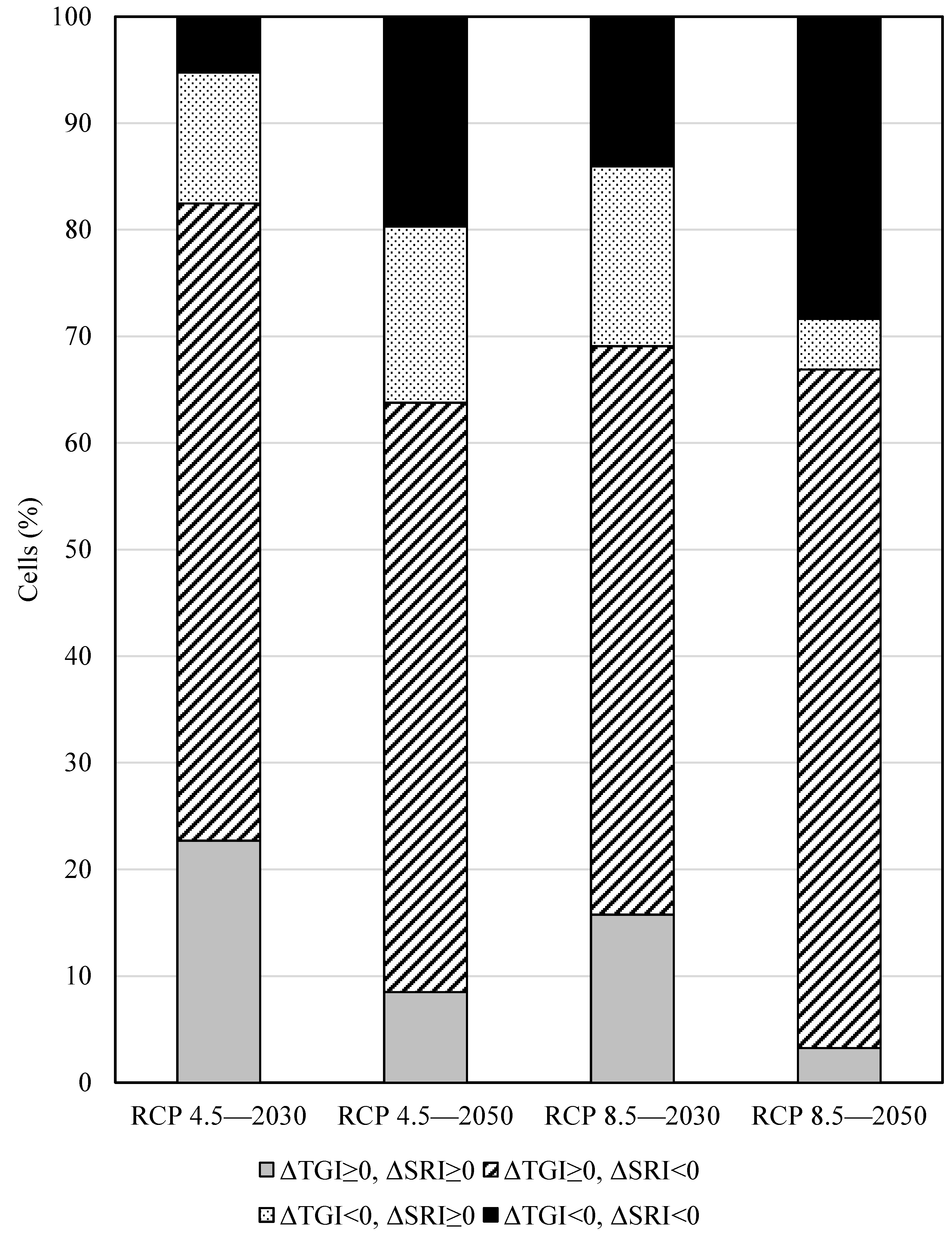
| SRI | TGI | SS | |
|---|---|---|---|
| Present | 33.48 ± 12.1 | 0.488 ± 0.26 | 7.66 ± 3.48 |
| RCP 4.5—2030 | 29.20 ± 10.8 | 0.637 ± 0.26 | 9.86 ± 4.82 |
| RCP 4.5—2050 | 24.11 ± 11.2 | 0.552 ± 0.30 | 6.37 ± 3.98 |
| RCP 8.5—2030 | 28.28 ± 10.8 | 0.560 ± 0.27 | 7.88 ± 4.16 |
| RCP 8.5—2050 | 20.27 ± 8.4 | 0.543 ± 0.29 | 6.13 ± 3.16 |
| Category | Predictor | Present | RCP 4.5—2030 | RCP 4.5—2050 | RCP 8.5—2030 | RCP 8.5—2050 |
|---|---|---|---|---|---|---|
| Temperature | Tavg | 12.295 ± 1.026 | −0.165 | 0.480 | −0.086 | 1.038 |
| (°C) | Tspr | 12.542 ± 0.845 | −1.178 | −0.362 | −0.956 | 0.105 |
| Taut | 13.439 ± 1.119 | 0.061 | 0.659 | 0.268 | 1.739 | |
| Tdif | 28.907 ± 1.672 | −1.768 | −2.263 | −1.425 | −0.854 | |
| Precipitation | Pavg | 103.307 ± 11.421 | −1.310 | 16.498 | 11.201 | 0.759 |
| (mm/month) | Pspr | 75.209 ± 16.594 | −2.317 | 17.513 | 2.498 | 11.806 |
| Paut | 96.332 ± 11.707 | −14.521 | −17.643 | −15.554 | −25.341 | |
| Pdif | 357.571 ± 51.327 | −22.945 | 94.094 | 51.414 | 41.158 | |
| Flow Rate | FRavg | 33.064 ± 69.280 | 3.713 | 13.111 | 10.824 | 14.847 |
| (m3/s) | FRspr | 15.618 ± 37.778 | 5.112 | 11.815 | 7.269 | 10.948 |
| FRaut | 41.648 ± 85.790 | 2.517 | −1.356 | 0.025 | −4.622 | |
| FRdif | 99.970 ± 211.498 | −5.399 | 49.179 | 40.278 | 63.992 | |
| Water Quality | TN | 2.487 ± 1.450 | 0.199 | 0.010 | 0.055 | 0.087 |
| (mg/L) | TP | 1.495 ± 14.033 | 0.493 | 0.010 | 0.165 | 0.152 |
| TSS | 22.514 ± 23.685 | 6.468 | 2.724 | 2.356 | 2.767 | |
| Topography | Elev | 201.07 ± 166.56 | - | - | - | - |
| Slope | 3.55 ± 3.09 | - | - | - | - |
| Han | Nakdong | Geum | Seomjin | Yeongsan | Total | |
|---|---|---|---|---|---|---|
| Present | −0.6901 | −0.6915 | −0.7164 | −0.8023 | −0.6981 | −0.6610 |
| RCP 4.5—2030 | 0.5094 | 0.6387 | 0.5693 | 0.4785 | 0.6306 | 0.5666 |
| RCP 4.5—2050 | 0.3703 | 0.4595 | 0.5399 | 0.3656 | 0.4392 | 0.4422 |
| RCP 8.5—2030 | 0.4655 | 0.5407 | 0.6174 | 0.3474 | 0.3559 | 0.4983 |
| RCP 8.5—2050 | 0.5153 | 0.5153 | 0.4868 | 0.5456 | 0.2937 | 0.4883 |
Publisher’s Note: MDPI stays neutral with regard to jurisdictional claims in published maps and institutional affiliations. |
© 2020 by the authors. Licensee MDPI, Basel, Switzerland. This article is an open access article distributed under the terms and conditions of the Creative Commons Attribution (CC BY) license (http://creativecommons.org/licenses/by/4.0/).
Share and Cite
Kim, Z.; Shim, T.; Koo, Y.-M.; Seo, D.; Kim, Y.-O.; Hwang, S.-J.; Jung, J. Predicting the Impact of Climate Change on Freshwater Fish Distribution by Incorporating Water Flow Rate and Quality Variables. Sustainability 2020, 12, 10001. https://doi.org/10.3390/su122310001
Kim Z, Shim T, Koo Y-M, Seo D, Kim Y-O, Hwang S-J, Jung J. Predicting the Impact of Climate Change on Freshwater Fish Distribution by Incorporating Water Flow Rate and Quality Variables. Sustainability. 2020; 12(23):10001. https://doi.org/10.3390/su122310001
Chicago/Turabian StyleKim, Zhonghyun, Taeyong Shim, Young-Min Koo, Dongil Seo, Young-Oh Kim, Soon-Jin Hwang, and Jinho Jung. 2020. "Predicting the Impact of Climate Change on Freshwater Fish Distribution by Incorporating Water Flow Rate and Quality Variables" Sustainability 12, no. 23: 10001. https://doi.org/10.3390/su122310001