A Kalman Filter-Based Approach for Online Source-Term Estimation in Accidental Radioactive Dispersion Events


Department of Energy, Politecnico di Milano, Via La Masa 34, 20156 Milano, Italy
*
Author to whom correspondence should be addressed.
Sustainability 2020, 12(23), 10003; https://doi.org/10.3390/su122310003
Submission received: 10 November 2020
/
Accepted: 25 November 2020
/
Published: 30 November 2020
(This article belongs to the Special Issue Sustainability in Innovative Nuclear Fission/Fusion Systems and Related Fuel Cycles)
Abstract
:In the present work, a online data assimilation approach, based on the Kalman filter algorithm, is proposed for the source term reconstruction in accidental events with dispersion of radioactive agents in air. For this purpose a Gaussian plume model of dispersion in air is embedded in the Kalman filter algorithm to estimate unknown scenario parameters, such as the coordinates and the intensity of the source, on the basis of measurements collected by a mobile sensor. The approach was tested against pseudo-experimental data produced with both the Gaussian plume model and the Lagrangian puff model SCIPUFF. The results show the good capabilities of the proposed approach in retrieving the values of the unknown parameters when (i) one or more release parameters are poorly known and (ii) a sufficient number of experimental measurements describing the evolution of the dispersion process can be collected in a short time by means of mobile sensors. Thanks to its flexibility and computational efficiency, and due to the exploitation of the Kalman filter potentialities through the use of a simplified model of dispersion in air, the proposed approach can constitute a useful tool for the management of emergency scenarios.
1. Introduction
When dealing with the analysis of accidental atmospheric releases of radionuclides, or more in general, hazardous contaminants, predictive computational models constitute essential tools to provide decision-makers with quantitative information for both emergency operations and post-accident management [1]. Typical applications involve local- to global-scale scenarios, with time scales which can range from a few hours to several months. The choice of the most appropriate modelling approach depends on the complexity of the scenarios, in terms of computational effort, amount of required input data and spatial and temporal scales involved.
Microscale scenarios (<1–2 km) are strongly affected by the interaction of atmospheric flows with surface irregularities, such as buildings and obstacles in general. This can lead to large inaccuracies in the predictions, if detailed geometry is not taken into account. Moreover, as numerical weather prediction (NWP) tools do not have adequate resolution for microscale scenarios, some effort for the determination of the wind field is often required as well. For these reasons, approaches based on computational fluid dynamics (CFD) were adopted in recent years to deal with miscroscale scenarios [2,3,4]. In spite of their good accuracy, the complexity of such tools and their computational requirements are incompatible with large scales and real-time applications. Different approaches are usually adopted for mesoscale and macroscale scenarios. In the Eulerian approach, transport equations are discretised and numerically approximated [5,6]. In the Lagrangian approach, a large number of pseudo-particles of the released agent are tracked along their trajectories [7,8]. Such trajectories are determined as the result of two contributions, i.e., deterministic advection by the wind field and stochastic diffusion due to turbulence. In both Eulerian and Lagrangian approaches, the wind field is usually obtained from standard NWP models. Despite their simplicity, Gaussian dispersion models [9] are also widely employed and are among the most commonly used tools in regulatory air dispersion modelling for fast screening purposes at different scales.
Regardless of the choice of the modelling approach and the spatial or temporal scales of the scenario, a fundamental issue with the analysis of accidental events can be the lack of information regarding the intensity and location of the source of release, i.e., the so-called source term. One may think of a nuclear accident, where it is generally hard to estimate the amount of the release of radioactive agents directly from the plant inventory, or a more generic radiological event in which even the location of the source might be poorly known. In such situations, data coming from concentration or activity measurements collected by on-site sensors might be exploited to obtain estimates of the unknown quantities.
The general problem of estimating one or more parameters characterising a system from observed data is commonly known as an inverse problem [10]. Inverse problems arise very often in the field of atmospheric releases of contaminants, in which they usually take the name of source term estimation (STE) problems. The aim of a STE problem is to estimate the main parameters which define the source of the release, i.e., its location and intensity. The STE problem has been subject of intense study and the potential exploitation of measurements collected by sensors has attracted great interest in recent years [11]. In general, source term estimates are intended to be used as input for further analyses, either on-site, to provide a fast local characterisation of the scenarios, or off-site, to feed more sophisticated long-range models.
Most of STE approaches are based on the minimisation of an objective function, which gives a measure of the discrepancy between observed data and predictions obtained with the adopted model of dispersion in air. Methods have been proposed which employ simple analytical dispersion models [12,13], or more complex modelling approaches, e.g., the advection-diffusion equation [14,15], CFD [16] and other off-the-shelf tools like the SCIPUFF Lagrangian-puff model [17,18]. Bayesian techniques, which are widely adopted, are based on a statistical approach in which inherent uncertainties affecting measurements or the adopted model of dispersion in air are taken into account together with prior information. This provides posterior statistics about the estimated quantities from which confidence regions can be obtained. Most of the literature deals with steady-state, single source problems. Some approaches have also been proposed for multiple sources [19] or time-dependent scenarios [20]. Estimated quantities usually include source term parameters, such as its location in a 2D or 3D domain and its intensity, with meteorological data given as input. In some cases wind and turbulence parameters have been estimated as well, e.g., by Wade and Senocak [21] and Senocak et al. [22].
The majority of the literature deals with static sensor networks where the sampling locations are either constrained by available data sets or selected a priori. When mobile sensing devices are considered, the additional problem of the choice of the sampling strategy must be addressed. This enables the use of all the available information (dispersion models, current estimates, previous observations) to steer the sampling procedure towards locations where more informative observations can be collected. Common approaches to address this problem include the maximisation of some kind of predicted information gain [23] or of some measure of the mutual information between model output and measurements [24].
In the present work, an approach based on Kalman filter embedding of a Gaussian plume model is proposed for the online estimation of the location and intensity of a single source of release in a 3D domain, by resorting to the employment of mobile sensors. According to the proposed approach, measurement data collected by a sensor can be processed recursively, allowing the online updating of the estimated quantities. Such an online data collection and update approach also enables a less strict sampling strategy, where the sensor path is not established a priori but can be controlled by the source estimation algorithm. This strategy can be of interest for emergency scenarios, where data are made available as soon as they are collected and fast estimation techniques are essential. Knowledge about the source term (and any other uncertain parameter) can be therefore improved each time new observations made available by sensors are assimilated by the algorithm. Kalman filtering is particularly suited for any time evolution model for which an analytical formulation—or at least a time-stepping operator—is given. A similar approach was proposed by Drews et al. [25], who considered a static sensor network to estimate the intensity of a single-source release from a known location. Even though in the present work a simple fast-running Gaussian dispersion model has been employed, the approach is indeed quite general and can be employed with more sophisticated atmospheric dispersion models as well. A case study, describing the dispersion at the microscale of a non-reactive agent released by a steady state single point source, was selected to test the methodology. Some release parameters were treated as unknown and subject to estimation. Two series of tests are presented: in the first one, pseudo-experimental dispersion data were produced with the Gaussian plume model, to check the correct implementation of the methodology and the consistency of estimation results. In the second series, the SCIPUFF Lagrangian puff model was used to produce pseudo-experimental dispersion data.
The paper is organised as follows: in Section 2 the adopted methods and modelling strategies are presented. More specifically, Section 2.1 reports brief descriptions of the employed atmospheric dispersion models, namely, the Gaussian plume model and the SCIPUFF Lagrangian puff model. Section 2.2 gives basic descriptions of the Kalman filter algorithm and the related techniques, upon which the proposed data assimilation approach is based. In Section 2.3 the proposed source term estimation algorithm is presented. The case study selected for the verification of the proposed approach is then described in Section 2.4. In Section 3 the results of the tests on the case study are reported and discussed. Conclusions are presented in Section 4, together with possible suggestions for further work.
2. Materials and Methods
2.1. Atmospheric Dispersion Modelling
2.1.1. The Gaussian Plume Model
Gaussian plume models comprise a family of simplified models which are based on an analytical solution of the atmospheric advection-dispersion problem. For a detailed discussion on Gaussian models from basic formulations to more sophisticated implementations, the reader may refer to [26]. Fundamental equations are usually derived under the following assumptions:
- (i)
- The source of contaminant can be considered as localised in a single point (point source approach).
- (ii)
- The release rate from the source is continuous and constant in time.
- (iii)
- The wind speed and direction are both constant in time and uniform in space.
- (iv)
- Atmospheric turbulence is constant in time and uniform in space.
Following the convention by which the coordinates respectively indicate the downwind, crosswind and vertical axes directions, the basic formulation reads:
where c is the concentration at a given point (g m−3). The origin of the coordinate system is placed at ground level in correspondence with the source location. The term represents the downwind dilution:
where S and u are the source release rate (g s−1) and the wind speed at release height (m s−1), respectively. The terms and represent the crosswind and vertical dilution:
where is the source release height (m), while and are the dispersion parameters in the y and z directions (m).
The and parameters are used to model the broadening of the Gaussian plume due to atmospheric turbulence, as it drifts away from the source point. It follows that appropriate empirical correlations must be used to assess and as functions of x and weather conditions. Among available parametrisations of various complexity, the ones based on atmospheric stability classes are still widely adopted due to their simplicity. The most commonly used classification of atmospheric stability is the one developed by Pasquill [27] and Gifford [28]. The original empirical correlations are commonly used in the formulation proposed by Briggs [29]:
where , , , , , are empirical constants depending on the Pasquill–Gifford stability class.
The decay term D is commonly used as a simple correction factor to model exponential decay, or more in general, first-order chemical reactions [30]:
where is the decay rate (s−1). When radioactive agents are considered, the decay term D is simply neglected if the decay rate of the radionuclide is sufficiently small according to (7).
2.1.2. The SCIPUFF Model
SCIPUFF (second-order closure integrated PUFF) is a Lagrangian transport and diffusion model for atmospheric dispersion applications [31]. The technique employed to solve the transport equations is the Gaussian puff method in which a collection of 3D puffs is used to represent an arbitrary time-dependent release. The turbulence parametrisation used in SCIPUFF is based on a second-order turbulence closure theory, providing a direct connection between measurable velocity statistics and the predicted dispersion rates. The Lagrangian approach allows an accurate treatment of a wide range of length scales. This range may extend from the microscale to the macroscale, namely, from a few tenths of a metre up to continental or global scales. The meteorological input required by SCIPUFF ranges from simple input parameters, like single wind vectors, to observational data such as single wind measurements or multiple profiles. Observations can include turbulence measurements and boundary layer parameters such as mixing-layer height or Pasquill–Gifford stability class. Alternatively, 3D gridded wind and meteorological fields generated by a prognostic weather model may be used as input.
2.2. The Kalman Filter Algorithm
2.2.1. The Original Formulation
The Kalman filter (KF) is a widely employed data assimilation algorithm, originally developed as a recursive predictor-corrector state estimator [34]. It is based on a state space representation of the mathematical model under analysis, in which the state variables of the system are included in a state vector , while its observable quantities are included in an observable vector . The subscript t typically denotes a time instant, but more generally it may simply represent a sequential iteration index. The system is thus described by the following equations:
where and represent two generic, nonlinear, possibly time-dependent, deterministic operators: the state Equation (8) provides the time evolution of the system, while the observation Equation (9) links the state of the system to the observable quantities. The terms and are respectively the so-called process noise and measurement noise. They consist of two mutually uncorrelated stochastic vector variables and represent all uncertainties and non-deterministic effects affecting the model. The system model thus comprises a deterministic and a stochastic part, such that the state becomes a stochastic variable itself subjected to a certain probability distribution.
The original formulation of the KF is based on the following assumptions:
- (i)
- the stochastic vector variables and follow multivariate Gaussian probability distributions, each characterised by zero mean and covariance matrices and , respectively (i.e., , , );
- (ii)
- the stochastic vectors variables and are not cross-correlated, i.e., , for ;
- (iii)
- the operators and are linear.
Such assumptions ensure that the stochastic variables involved in the algorithm are Gaussian and that the KF provides a least-squares best estimate of the state , in terms of its expected value and covariance matrix . While conditions (i) and (ii) are quite straightforward (at least in lack of better knowledge), condition (iii) is not easily satisfied, especially when model parameters are included in the state vector. In such cases the expressions and require modifications which make them nonlinear.
Under the hypothesis of model linearity, (8) and (9) may be written as follows:
where and are linear, still possibly time-dependent operators.
To introduce the KF equations, it is assumed, at a given instant t, to possess the following pieces of information:
- (i)
- the estimate of the system state at the previous instant is characterised by an expected value and a covariance matrix ;
- (ii)
- one or more measurements have been performed on the system at time t, yielding the measurement vector .
Then, the KF equations consist in a prediction step in which the state is propagated forward in time on the basis of the model:
and a correction (or update) step in which measurements are assimilated and used to adjust the prediction:
where the optimal Kalman gain is defined as:
The matrix is regarded as a gain, as it determines the degree to which the discrepancy between measurements and model prediction is amplified to correct the prediction itself. The value assumed by the gain matrix at each iteration is determined by the combination of the uncertainties associated with the state after prediction and to the measurements. It follows from (14) and (16) that, when the uncertainty associated with the measurements is ideally made very large or very small, the updated estimate respectively tends to and . Analogous statements hold also for the covariance matrix .
Given that (12) to (16) allow one to propagate recursively the estimate of the state from instant to t by assimilating the data collected at time t, the KF algorithm needs to be initialised at t = 0. Initial conditions and for the state of the system must therefore be provided. They can result from previous analyses, from expert opinions or from any other source of information. When no reliable information is given, rough or tentative initial estimates can be used by specifying relatively large initial covariance, as the KF will forget about initial estimates after few iterations.
2.2.2. The Extended Kalman Filter Algorithm
As most practical applications involve nonlinear model equations, the assumptions described in the previous section do not hold and (12) to (16) can not be used to propagate the state of the system. If nonlinearities in the model are not too strong, one common solution to the nonlinear estimation problem consists of deriving linearised versions of the operators and . This leads to the so-called extended Kalman filter (EKF) equations [35] for the prediction step:
the correction step:
and the Kalman gain:
The linear operators and are here defined as the following Jacobian matrices:
When nonlinearities are too strong, the EKF may yield poor estimation results. For nonlinear models the EKF is not in general an optimal estimator and poor initial estimates may cause the algorithm to diverge. As alternatives to the standard EKF, more advanced approaches are available, e.g., the iterated EKF [35], in which the equations are solved by iteratively modifying the linearisation point. This limits the error introduced by linearisation at the expense of increased computational burden. Another example is the unscented Kalman filter (UKF) [36], in which, rather than approximating the model equations with some linearised versions, the probability density functions of the involved quantities are directly approximated by choosing a small set of sampling points and then nonlinearly propagated. Besides yielding better estimation results in many applications, the UKF can be particularly useful in all cases where the Jacobians are not available or their computation proves to be too complex or demanding. The present works employs the EKF algorithm to deal with the nonlinearities of the Gaussian dispersion model. Jacobian matrices are evaluated numerically.
2.3. Architecture of the Proposed Source Term Estimation Algorithm
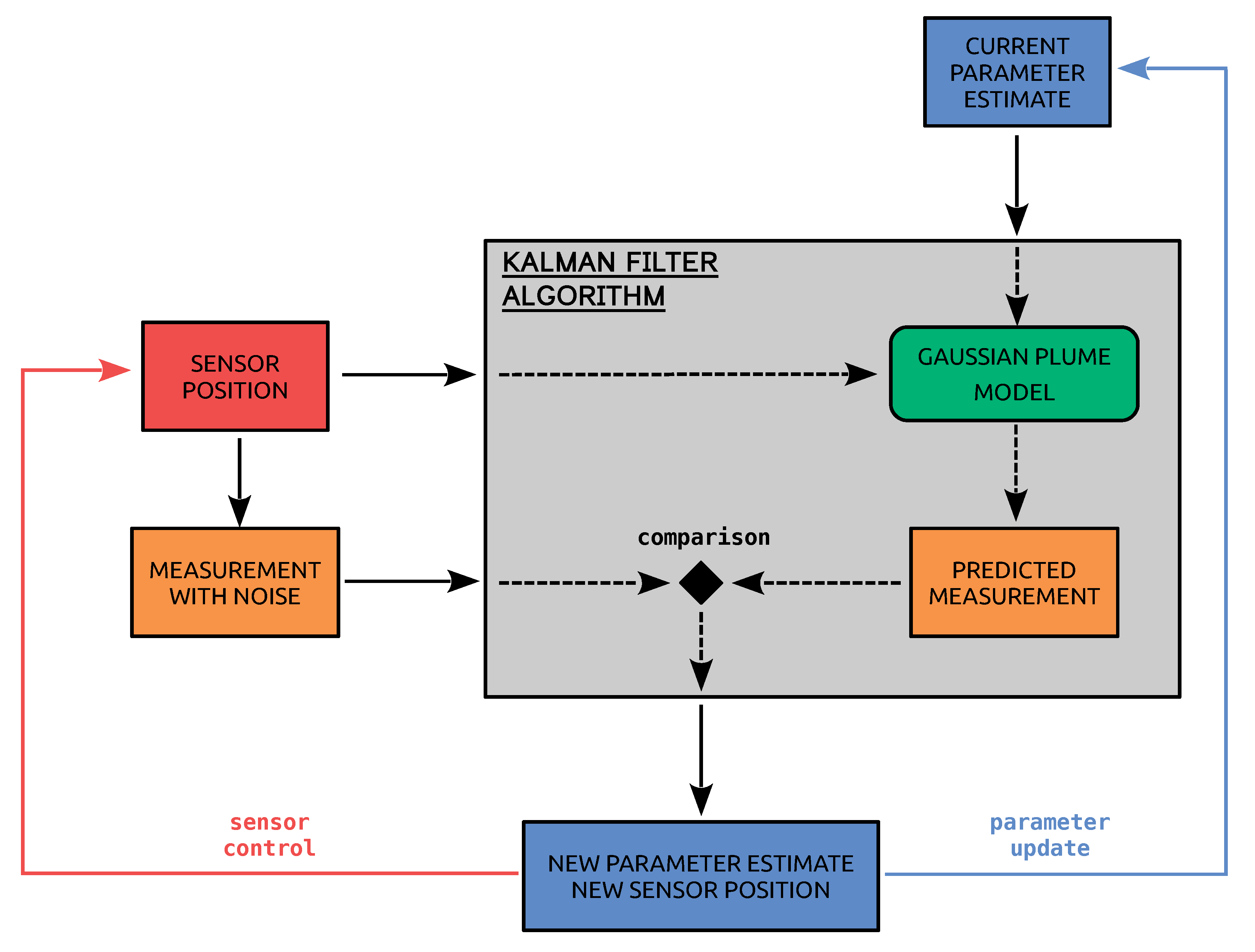
A conceptual scheme of the here proposed source term estimation algorithm is depicted in Figure 1. The proposed online data assimilation approach for the source term estimation is based on the Kalman filter in which a Gaussian plume dispersion model is embedded. Model predictions are compared with measurements to perform the online update of estimated quantities. The algorithm can also make use of the most recent estimates of the unknown parameters to control mobile sensors placement. A simulation loop provides measurement predictions, the current estimates of the parameters and the current position of the sensor, while a control loop drives the sensor based on current parameters estimates. Information on the sensor noise level is used to weigh the contribution of experimental observations during the update of the estimates. The approach focuses on single-source steady-state scenarios that fulfil the hypotheses under which the Gaussian plume model is derived.
2.3.1. Parametrisation of Atmospheric Stability
Regarding the parametrisation of atmospheric stability, and are computed as functions of the downwind distance x and of a stability class parameter , here defined as a proxy of the so-called atmospheric stability class. The parameter is used to evaluate the empirical coefficients appearing in (5) and (6) by piece-wise linear interpolation of the values from Briggs [29]. The coefficients of the six original stability classes from Pasquill [27] and Gifford [28] are hence interpolated to provide a continuous parametrisation using a single parameter (Table 1).
2.3.2. Embedding in the Kalman Filter Algorithm
The Kalman state vector is built as:
where are the unknown parameters of the Gaussian model which are to be estimated. The maximum size of the state vector is , which corresponds to all the parameters being regarded as unknown, i.e., the source location coordinates and release rate, the wind velocity and direction and the stability class parameter:
The actual composition of the state can be modified from one case to another, depending on which parameters are known.
The state estimate is updated, starting from an initial guess, using the EKF equations as described in Section 2.2.2. The time evolution operator in (8) is the identity, since the process is assumed to be (statistically) steady-state:
where I is the identity matrix. The observation Equation (9) is derived from the Gaussian model equations:
where is the number of observations made independently at time t. The function therefore depends on time, as the positions (and possibly also the number) of the observations can vary from one iteration to another. The Jacobian matrix is easily obtained at each iteration by numerical differentiation of (28).
2.3.3. Sampling Strategy
The positions of the observations are updated at each iteration taking into account the current estimate of the source location. The employed sampling strategy keeps the sensor roughly at a fixed downwind distance from the estimated source location, i.e., on the plume centreline and at the source release height:
where the coordinates are expressed with respect to the Gaussian model reference system. Since the concentration decays rapidly when moving from = in the y and z directions, the broadening of the plume is exploited to avoid measurements in regions where the concentration is low compared to the measurement noise. At each iteration is determined together with additional measurement positions. With respect to , two additional measurements are made in each direction (downwind, crosswind, vertical):
where , and are constant values. The number of observations at each iteration, in this case, is therefore . This is done to ensure better measurement statistics and to acquire information in all directions.
2.4. Case Study
A micro-scale dispersion scenario characterised by a constant and point-source release is considered. The size of of the considered domain is 500 × 500 × 25 m. The source coordinates are expressed in a generic reference system and the source intensity S is given in arbitrary units, as reported in Table 2. The wind speed u is set to 5 m s−1 (constant and uniform), while for atmospheric stability, three different scenarios are selected which correspond to the second, third and fourth (i.e., B,C,D) stability classes from the Pasquill–Gifford classification. The corresponding dispersion coefficients are typical of moderately unstable, slightly unstable and neutral atmospheric conditions respectively [29]. SCIPUFF observational data assimilation features are exploited to prescribe atmospheric stability according to the Pasquill–Gifford scheme. It is further assumed that radioactive decay is negligible with respect to the time scales under consideration. Albeit based on a different kind of parametrisation with respect to the one adopted in this work, the SCIPUFF model can use Pasquill–Gifford classes to specify turbulent diffusion. Non-integer values are accepted by the program and treated by interpolation as well.
The proposed estimation algorithm was verified by running two series of tests wherein pseudo-experimental data were produced by means of dispersion models. The proposed approach was first tested using pseudo-experimental data produced with the Gaussian plume model (Section 3.1), and then with pseudo-experimental data generated by means of the SCIPUFF Lagrangian puff model (Section 3.2). The values adopted for the sampling parameters are listed in Table 3. The quantity defines the standard deviation of the measurement noise. It is used to build the measurement noise covariance matrix:
where I is the identity matrix of size q. It is therefore assumed for simplicity a constant fixed measurement noise for all observations, with no correlation between observations taken at different positions within the same algorithm iteration. The same standard deviation is used to sample random additive noise from a zero-mean normal distribution, which is added to each simulated measurement.
The wind speed u and angle are assumed known. The state vector is therefore built as:
The Kalman filter needs the definition of the process noise covariance matrix . There are no general rules for its choice. In this work, a diagonal matrix is used:
with , where for the present tests
The choice of such values is somewhat arbitrary. Listed values where chosen to provide satisfactory dynamical properties for the state estimates. They can be varied in a certain range with no significant consequences on the convergence properties of the algorithm, but larger values can lead to instability and divergence of the state estimate. On the other hand, smaller values lead to very slow convergence. It is worth remarking that, even though has a direct impact on Kalman filter equations—in particular on the definition of the Kalman gain in (21)—many applications are found in which process noise is not needed to drive the data assimilation process. In this case, however, model equations are such that state-to-output sensitivity is not large enough and process noise is needed. Setting its covariance to zero would result in no state update and the estimation algorithm would get stuck immediately.
3. Results
The proposed approach has been first tested using pseudo-experimental data generated by the Gaussian plume model (Section 3.1), then with data generated by means of the SCIPUFF model (Section 3.2). The source estimation algorithm is initialised with the same data in both the series of tests. Four different cases have been considered corresponding to different initial guesses of the release source coordinates and . For each of such cases, two possible values of the release source height are considered. To simplify the analysis, a single initial guess of the release source intensity and of the atmospheric stability class parameter is considered for all tests. Initial conditions for the quantities to be estimated are reported in Table 4. The values reported for , and refer to the initial “errors” with respect to the true values of Table 2, while and are expressed in absolute terms. Chosen values for and only represent positive initial errors, but the symmetry of the case study scenario makes the choice of the sign equivalent. Moreover, little confidence is given to the initial estimates, so that the algorithm is not dependent on the initial guesses for the state covariance matrix. The values adopted for the initial state covariance matrix are therefore omitted.
3.1. Verification against Pseudo-Experimental Data Generated with the Gaussian Plume Model
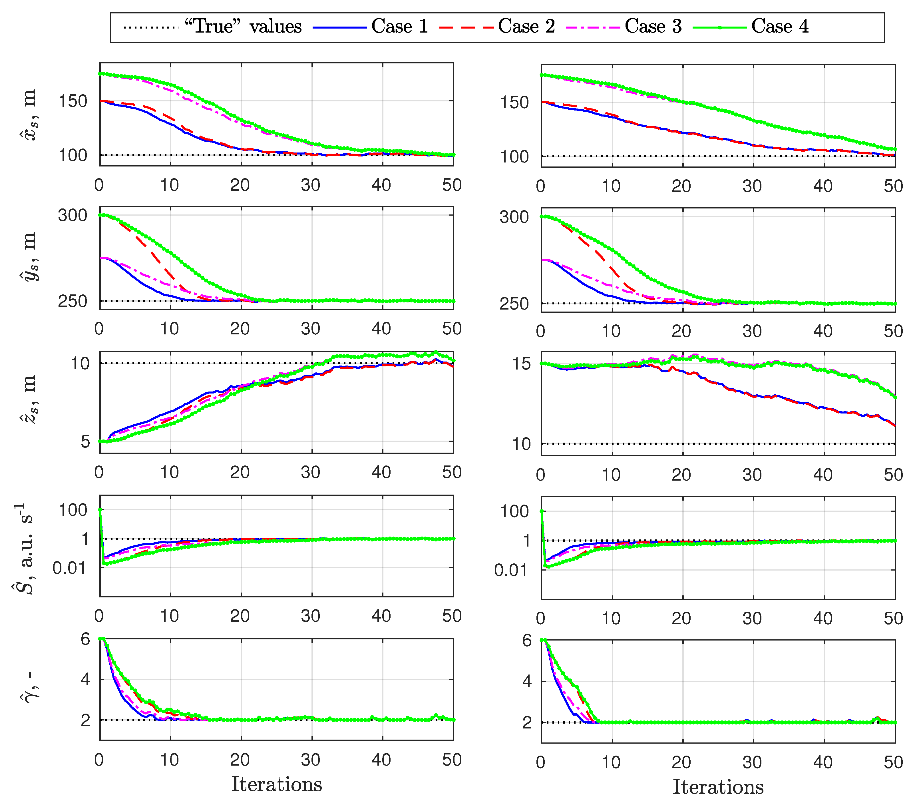
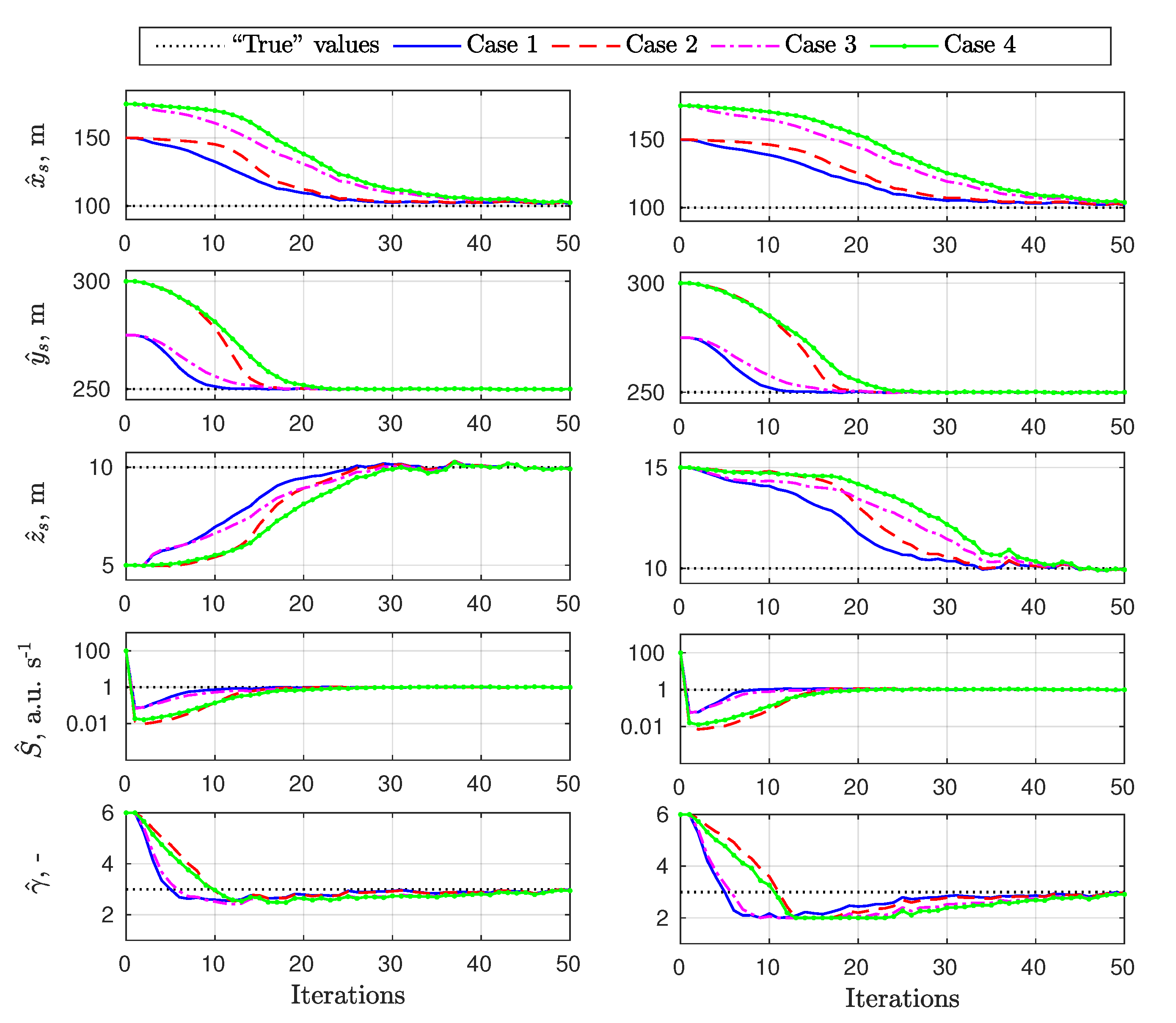
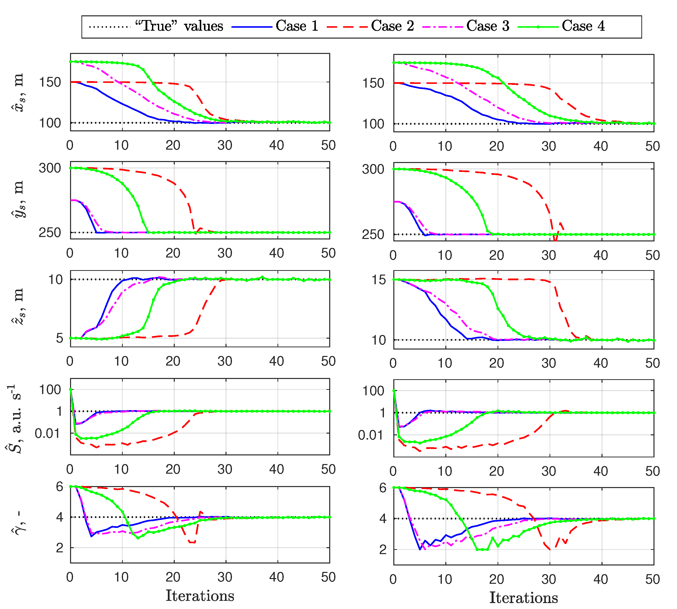
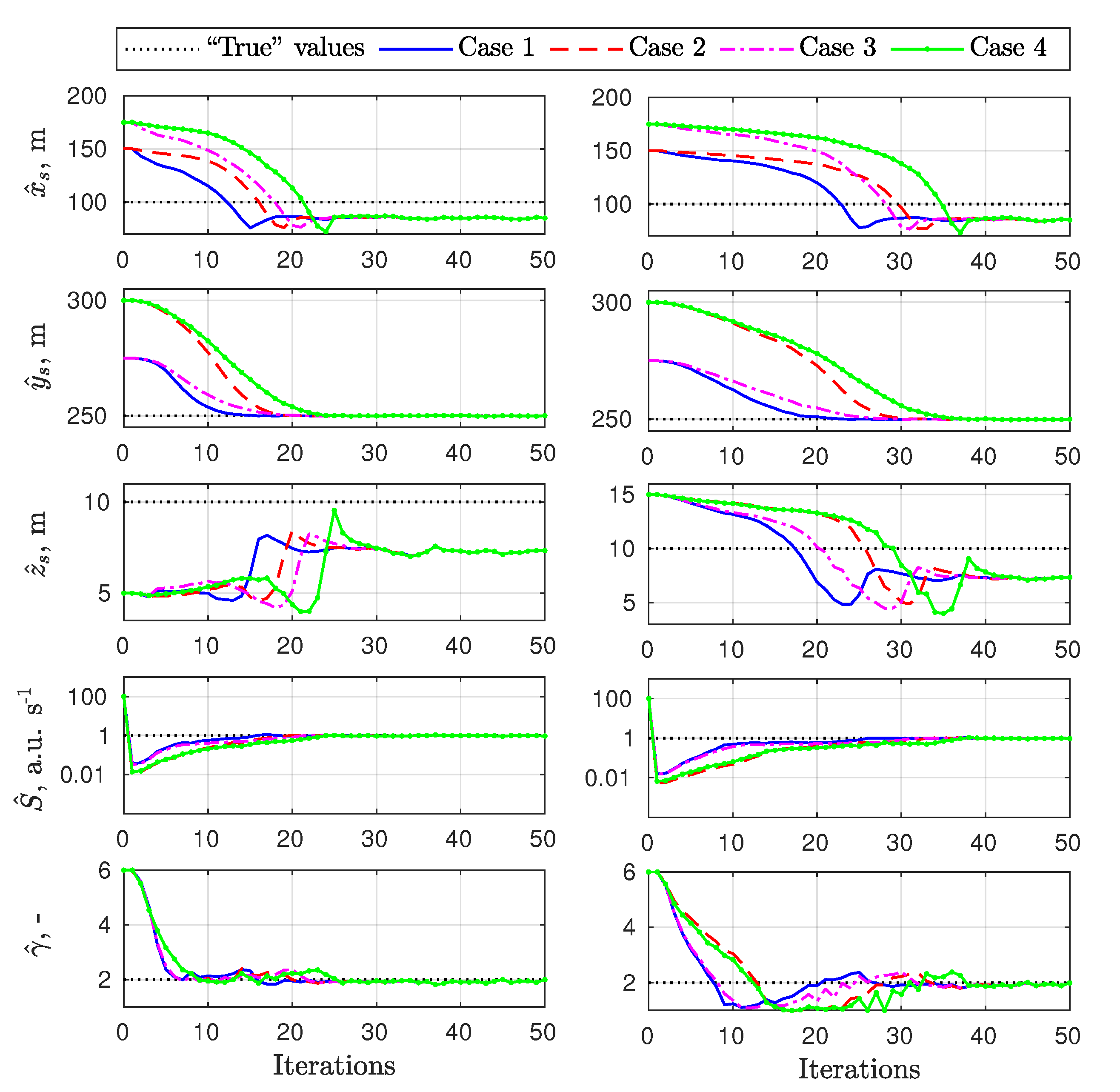
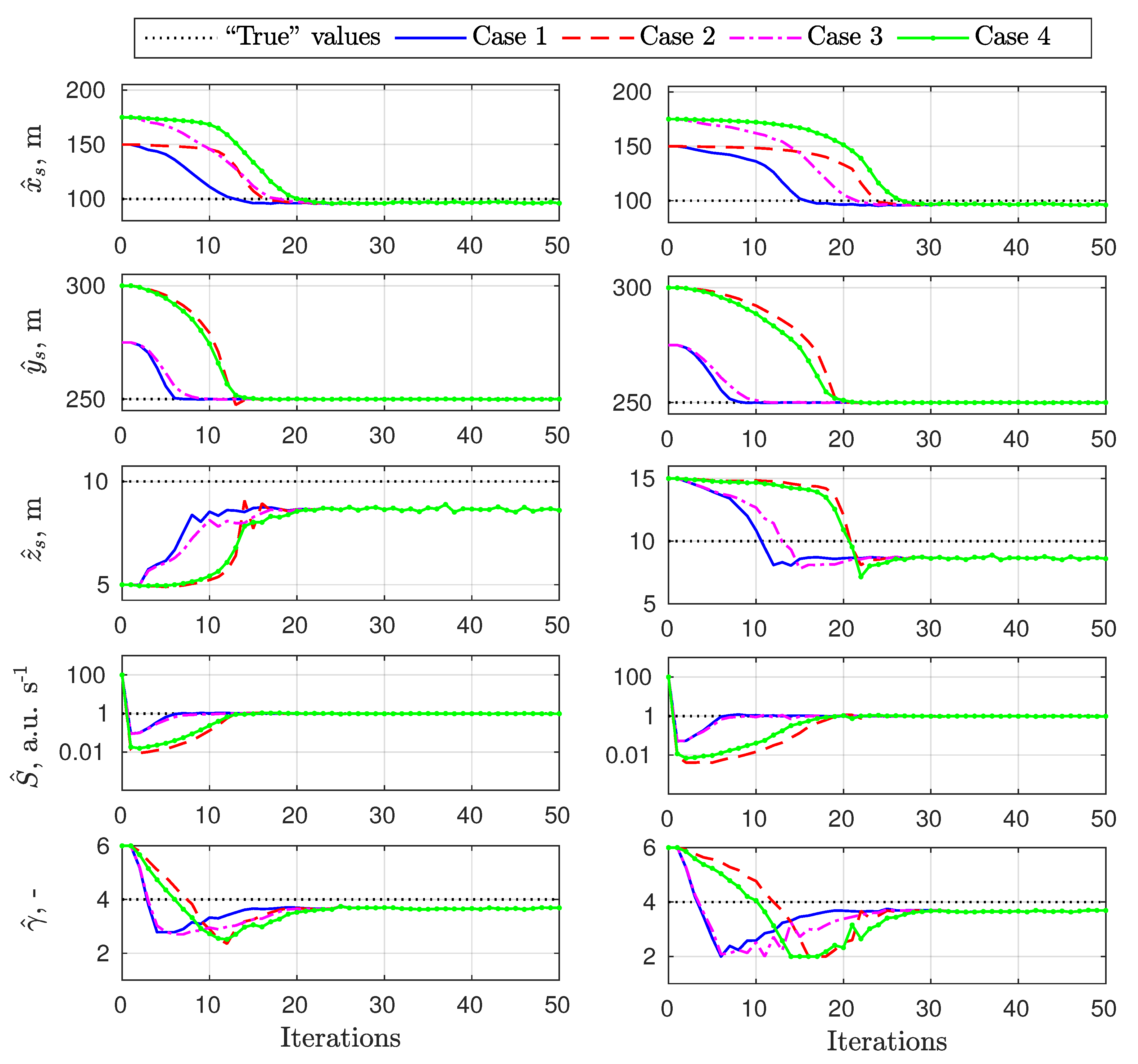
The evolution of state estimates along algorithm iterations for the 3 selected case-study values of the atmospheric stability class parameter (Table 2) are shown in Figure 2, Figure 3 and Figure 4 respectively. In almost all simulated cases, the algorithm shows its capability to retrieve the “true” parameter values in a reasonable amount of iterations (less than 50). Using the prior information on the measurement noise, the Kalman filter approach is able to adapt to the magnitude of the measured concentrations. Closer iterations are therefore made when noise is more significant, to collect more information. As the stability class parameter shifts towards 2 (class B), a generally slower convergence is observed. This is understandable since more unstable atmospheric conditions lead to smoother concentration profiles, with less information to be extracted from concentration gradients at each iteration. As a result, more measurements are needed for the algorithm to converge. This is particularly evident in Figure 2, where the estimate of the height of the source, , has not reached convergence yet after 50 algorithm iterations. It is also noted that the linear dependence of the observation equation on the source intensity S is exploited by the model, as the estimate is readily decreased by several orders of magnitude after very few iterations. Even though the initial guess was overestimated by two orders of magnitude, the algorithm at the end is able to converge to the “true” value. The slower convergence of the parameter estimates in case 2 and case 4 is clearly visible, especially in Figure 4. Apart from convergence rates, the overall dynamics of the estimates is similar for all cases with the same value of , but seems to depend in some way on the atmospheric stability conditions. Even though the final convergence is not hindered, this behaviour could suggest a non-optimal choice of the process noise covariance matrix for the specific cases and that an automatic scenario-dependent choice of such parameters could improve algorithm dynamics.
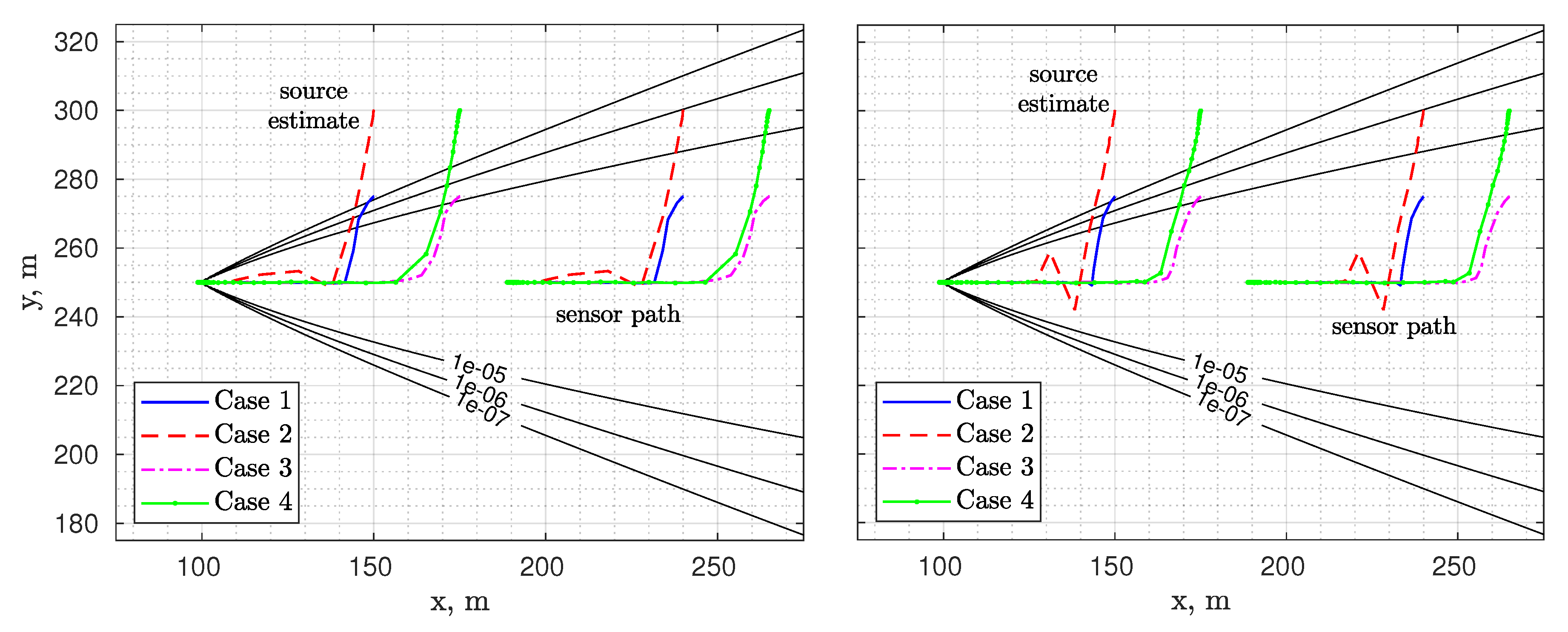
In Figure 5 are shown the trajectories in the x-y plane of both the mobile sensor position and the source estimate along iterations. For brevity, only results for the case with are reported. Due to the simple feedback strategy employed, the sensor path coincides with the source estimate path shifted by in the x direction. Contour plots at are added as well to characterise the concentration field due to the “true” parameter values. Contour values for concentrations of 0.1, 1 and 10 times the measurement noise are shown. The 4 test cases were chosen, as reported in Table 4, to span a wide region and to make the mobile sensor explore regions where the measurement noise is comparable in magnitude to the exact concentration values.
3.2. Verification against Pseudo-Experimental Data Generated with the SCIPUFF Model
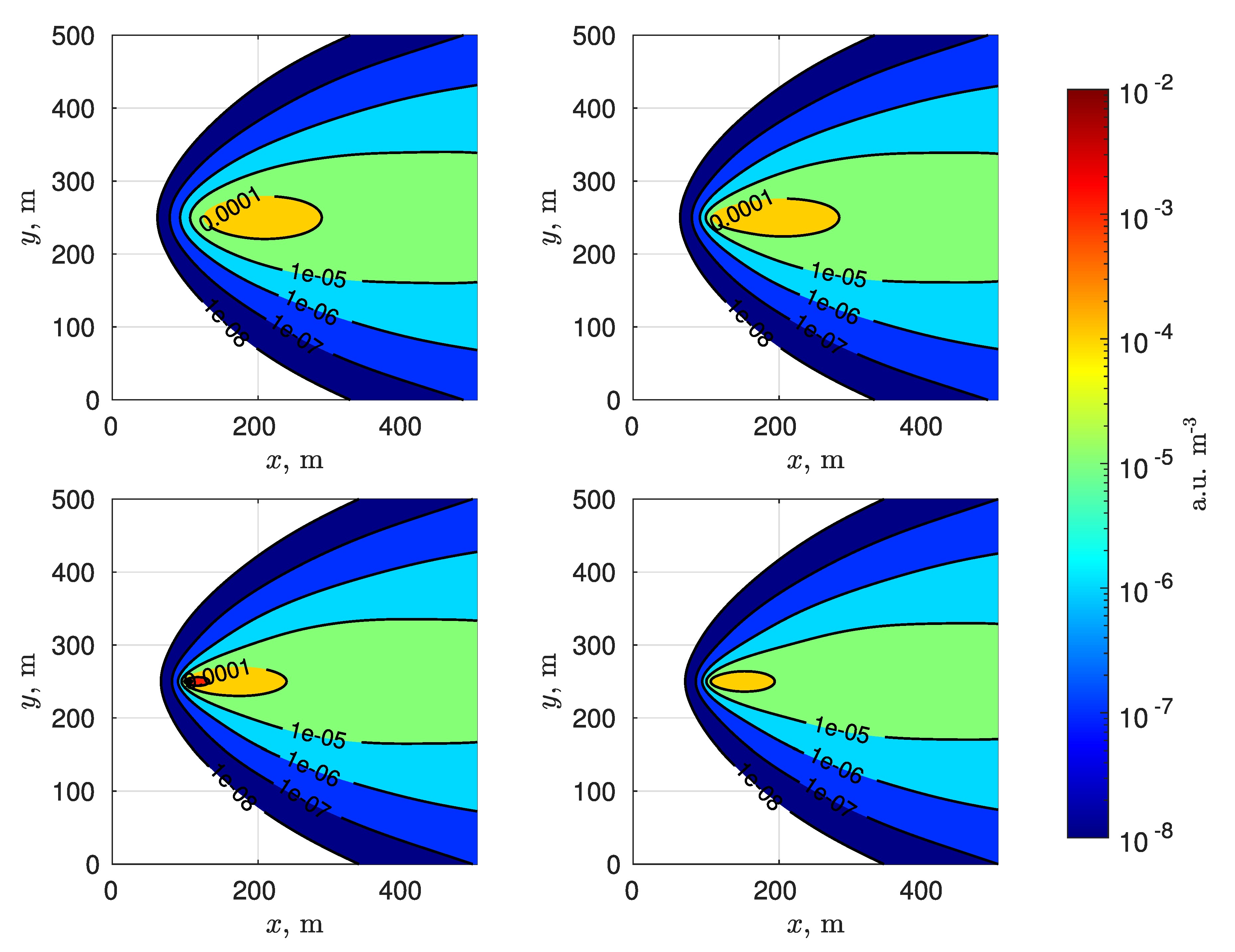
To test the capability of the proposed source term estimation algorithm based on the Gaussian plume dispersion model, pseudo experimental data have been produced by means of the SCIPUFF Lagrangian puff model, with the purpose of employing a more realistic set of dispersion data obtained with a dispersion model different from the one embedded in the Kalman filter algorithm. Since the SCIPUFF model allows for the specification of meteorological field data from an arbitrary amount of input point measurements, a single measurement point is specified from which the model computes uniform and constant meteorological fields. In particular, the same wind speed and atmospheric stability class as in the previous cases (Table 2) are used. The PGT class which SCIPUFF accepts as input is a close relative of the parameter here used, but, since the model uses a different and possibly more complex parametrisation of atmospheric instability, perfect agreement between the models cannot be expected. Concentration data is computed and exported off-line from SCIPUFF on a 3D grid of m with uniform spacing of 1 m ( points). Data is then read online by the algorithm and linearly interpolated to provide a continuous 3D concentration field from which pseudo-experimental observations data are extracted. The concentration contour plots of the SCIPUFF simulation data for PGT class equal to 3 at 4 different heights are reported in Figure 6.
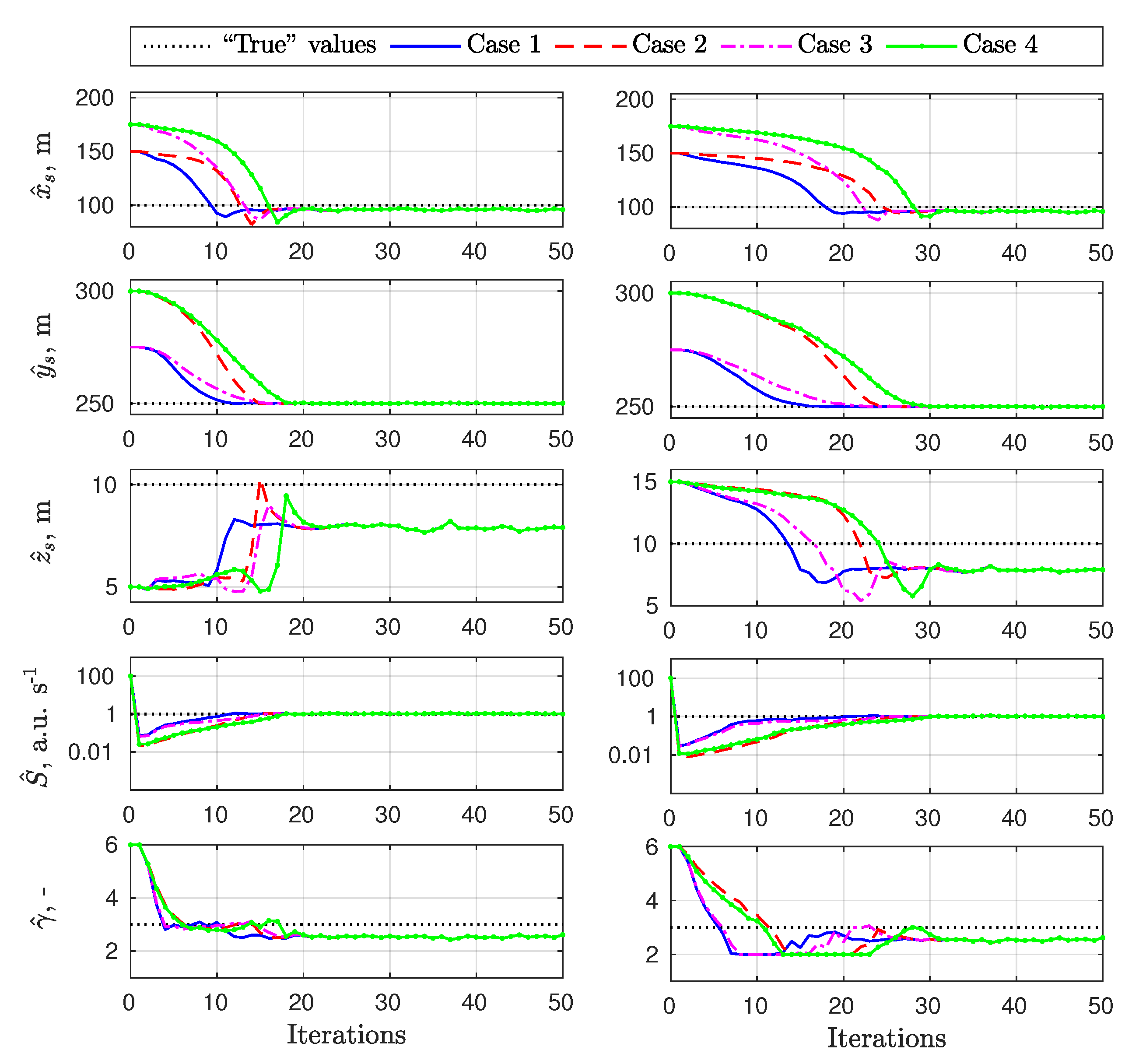
Figure 7, Figure 8 and Figure 9 show the source estimation results obtained using pseudo-experimental data from the SCIPUFF model, with PGT class respectively equal to 2, 3 and 4. Most of the observations on algorithm convergence made for the Gaussian plume cases are valid also in these cases. The proposed inversion methodology gives satisfactory results also when applied to pseudo-experimental data produced by a different dispersion model. The algorithm is able to identify, at least approximately, the source location and its intensity in all cases. This is particularly convenient since the atmospheric stability conditions are considered to be unknown and the Gaussian plume model and SCIPUFF model use different atmospheric stability parametrisations.
However, some discrepancies between the estimated quantities and the “true” scenario parameters are found. The estimated source height and stability class parameter are only approximately correct in most cases. The inaccuracies in retrieving the source height might be attributed to the poor approximation introduced by piece-wise linearly interpolated vertical concentration profiles obtained from SCIPUFF data. The uniform 1 m resolution of exported SCIPUFF data might be insufficient to properly describe vertical profiles, especially close to the source where concentration gradients are steeper. Estimation of with PGT class equal to B (Figure 7) shows the least satisfactory results, with an estimation bias of 10–15 m (consistent for all initial conditions). As pointed out earlier, no perfect match between the Gaussian and SCIPUFF dispersion models can be expected, with consequences on estimated values. The estimation algorithm relies on measurements collected quite far from the estimated source, so that some dependence on the local match between the models (and therefore on the distance from the estimated source) is expected.
4. Conclusions
An online source term estimation algorithm based on a Kalman filtering algorithm, within which is embedded a Gaussian plume model, is proposed. The unknown parameters of the Gaussian model constitute the state variables of the Kalman filter, while the Gaussian model equations are used to link the state variables to the observations which are fed to the algorithm. A mobile sensor is supposed to collect noisy measurements in a 3D scenario. In addition to more flexibility in the data sampling strategy, the use of mobile sensors enables a “feedback” mechanism to inform the sensor with updated information about the current source estimate. The proposed approach has been tested with simulated data coming from both the Gaussian plume model and the SCIPUFF Lagrangian puff model. It provides reliable estimates of the unknown state variables, including the source location and intensity, and the atmospheric stability class. Several cases have been tested, with different scenario parameters and initial estimates. In almost all cases the algorithm was able to retrieve satisfactory estimates of the parameter values after a few tens of algorithm iterations. Tests with Gaussian plume data showed almost perfect matches between “true” and estimated quantities, but tests with SCIPUFF data were affected by some inaccuracies that can be attributed to two main aspects. The first is the local discrepancy between the model employed to produce pseudo-experimental dispersion data and the model embedded in the estimation algorithm. The second is the spatial resolution of pseudo-experimental data fed to the algorithm, especially in the vertical direction. The overall accuracy was nevertheless good, as the x and y coordinates of the source location and the intensity were almost always correctly estimated. The estimated values of the stability class parameter are consistent with the PGT class adopted in SCIPUFF simulations. The approach was therefore demonstrated to be computationally efficient, and even though the quality of the estimates depends on the quality of the input data, it appears as a promising tool for the management of emergency radiological scenarios.
The approach is indeed very simplified and many assumptions were made. Further development and testing are therefore needed to prove its applicability in a real scenario. To extend the approach to non-uniform and possibly time-dependent scenarios, the adoption of more advanced tools, such as reduced order models (ROMs) and surrogate modelling techniques in general, could represent a viable option to embed complex and/or large models while preserving computational efficiency. Validation with experimental datasets, or at least cross-verification with other dispersion models, is foreseen to assess the limits of the approach with realistic data affected by noise.
Author Contributions
Conceptualisation, A.D.R., F.G. and A.C.; investigation, A.D.R.; supervision, F.G. and A.C.; writing—original draft, A.D.R.; writing—review and editing, A.D.R., F.G. and A.C. All authors have read and agreed to the published version of the manuscript.
Funding
This research received no external funding.
Conflicts of Interest
The authors declare no conflict of interest.
References
- Leelőssy, Á.; Lagzi, I.; Kovács, A.; Mészáros, R. A review of numerical models to predict the atmospheric dispersion of radionuclides. J. Environ. Radioact. 2018, 182, 20–33. [Google Scholar] [CrossRef] [PubMed]
- Tominaga, Y.; Stathopoulos, T. CFD simulations of near-field pollutant dispersion with different plume buoyancies. Build. Environ. 2018, 131, 128–139. [Google Scholar] [CrossRef]
- Lateb, M.; Meroney, R.; Yataghene, M.; Fellouah, H.; Saleh, F.; Boufadel, M. On the use of numerical modelling for near-field pollutant dispersion in urban environments-A review. Environ. Pollut. 2016, 208, 271–283. [Google Scholar] [CrossRef] [PubMed] [Green Version]
- de Sampaio, P.A.; Junior, M.A.; Lapa, C.M. A CFD approach to the atmospheric dispersion of radionuclides in the vicinity of NPPs. Nucl. Eng. Des. 2008, 238, 250–273. [Google Scholar] [CrossRef]
- Huh, C.A.; Lin, C.Y.; Hsu, S.C. Regional dispersal of Fukushima-derived fission nuclides by east-asian monsoon: A synthesis and review. Aerosol Air Qual. Res. 2013, 13, 537–544. [Google Scholar] [CrossRef]
- Mikkelsen, T.; Thykier-Nielsen, S.; Astrup, P.; Santabárbara, J.; Sørensen, J.; Rasmussen, A.; Robertson, L.; Ullerstig, A.; Deme, S.; Martens, R.; et al. MET-RODOS: A Comprehensive Atmospheric Dispersion Module. Radiat. Prot. Dosim. 1997, 73, 45–55. [Google Scholar] [CrossRef]
- An, H.Y.; Kang, Y.H.; Song, S.K.; Kim, Y.K. Comparison of CALPUFF and HYSPLIT models for atmospheric dispersion simulations of radioactive materials. J. Korean Soc. Atmos. Environ. 2015, 31, 573–584. [Google Scholar] [CrossRef] [Green Version]
- Connan, O.; Smith, K.; Organo, C.; Solier, L.; Maro, D.; Hébert, D. Comparison of RIMPUFF, HYSPLIT, ADMS atmospheric dispersion model outputs, using emergency response procedures, with 85Kr measurements made in the vicinity of nuclear reprocessing plant. J. Environ. Radioact. 2013, 124, 266–277. [Google Scholar] [CrossRef]
- Stockie, J. The mathematics of atmospheric dispersion modeling. SIAM Rev. 2011, 53, 349–372. [Google Scholar] [CrossRef]
- Tarantola, A. Inverse Problem Theory and Methods for Model Parameter Estimation; Society for Industrial and Applied Mathematics: Philadelphia, PA, USA, 2005. [Google Scholar]
- Hutchinson, M.; Oh, H.; Chen, W. A review of source term estimation methods for atmospheric dispersion events using static or mobile sensors. Inf. Fusion 2017, 36, 130–148. [Google Scholar] [CrossRef] [Green Version]
- Ristic, B.; Gunatilaka, A.; Gailis, R. Achievable accuracy in Gaussian plume parameter estimation using a network of binary sensors. Inf. Fusion 2015, 25, 42–48. [Google Scholar] [CrossRef]
- Borysiewicz, M.; Wawrzynczak, A.; Kopka, P. Bayesian-Based Methods for the Estimation of the Unknown Model’s Parameters in the Case of the Localization of the Atmospheric Contamination Source. Found. Comput. Decis. Sci. 2012, 37, 253–270. [Google Scholar] [CrossRef] [Green Version]
- Singh, S.K.; Rani, R. A least-squares inversion technique for identification of a point release: Application to Fusion Field Trials 2007. Atmos. Environ. 2014, 92, 104–117. [Google Scholar] [CrossRef]
- Keats, A.; Yee, E.; Lien, F.S. Bayesian inference for source determination with applications to a complex urban environment. Atmos. Environ. 2007, 41, 465–479. [Google Scholar] [CrossRef]
- Kumar, P.; Feiz, A.A.; Singh, S.K.; Ngae, P.; Turbelin, G. Reconstruction of an atmospheric tracer source in an urban-like environment. J. Geophys. Res. Atmos. 2015, 120, 12589–12604. [Google Scholar] [CrossRef] [Green Version]
- Sykes, R.I.; Parker, S.F.; Henn, D.S.; Gabruk, R.S. SCIPUFF-A generalized dispersion model. In Air Pollution Modeling and Its Application XI; Gryning, S.E., Schiermeier, F.A., Eds.; Springer: Boston, MA, USA, 1996; pp. 425–432. [Google Scholar]
- Allen, C.T.; Haupt, S.E.; Young, G.S. Source Characterization with a Genetic Algorithm–Coupled Dispersion–Backward Model Incorporating SCIPUFF. J. Appl. Meteorol. Climatol. 2007, 46, 273–287. [Google Scholar] [CrossRef]
- Annunzio, A.J.; Young, G.S.; Haupt, S.E. A Multi-Entity Field Approximation to determine the source location of multiple atmospheric contaminant releases. Atmos. Environ. 2012, 62, 593–604. [Google Scholar] [CrossRef]
- Zheng, X.; Chen, Z. Back-calculation of the strength and location of hazardous materials releases using the pattern search method. J. Hazard. Mater. 2010, 183, 474–481. [Google Scholar] [CrossRef]
- Wade, D.; Senocak, I. Stochastic reconstruction of multiple source atmospheric contaminant dispersion events. Atmos. Environ. 2013, 74, 45–51. [Google Scholar] [CrossRef] [Green Version]
- Senocak, I.; Hengartner, N.W.; Short, M.B.; Daniel, W.B. Stochastic event reconstruction of atmospheric contaminant dispersion using Bayesian inference. Atmos. Environ. 2008, 42, 7718–7727. [Google Scholar] [CrossRef] [Green Version]
- Ristic, B.; Skvortsov, A.; Walker, A. Autonomous search for a diffusive source in an unknown structured environment. Entropy 2014, 16, 789–813. [Google Scholar] [CrossRef] [Green Version]
- Madankan, R.; Singla, P.; Singh, T. Optimal information collection for source parameter estimation of atmospheric release phenomenon. In Proceedings of the 2014 American Control Conference, Portland, OR, USA, 4–6 June 2014; pp. 604–609. [Google Scholar] [CrossRef]
- Drews, M.; Lauritzen, B.; Madsen, H.; Smith, J.Q. Kalman filtration of radiation monitoring data from atmospheric dispersion of radioactive materials. Radiat. Prot. Dosim. 2004, 111, 257–269. [Google Scholar] [CrossRef] [PubMed]
- De Visscher, A. Air Dispersion Modeling: Foundations and Applications; John Wiley & Sons: Hoboken, NJ, USA, 2014. [Google Scholar]
- Pasquill, F. The Estimation of the Dispersion of Windborne Material. Meteorol. Manag. 1961, 90, 33–49. [Google Scholar]
- Gifford, F.A. Use of Routine Meteorological Observations for Estimating Atmospheric Dispersion. Nucl. Saf. 1961, 2, 47–51. [Google Scholar]
- Briggs, G.A. Diffusion Estimation for Small Emissions; Preliminary Report; Technical Report; NOAA Atmospheric Turbulence and Diffusion Laboratory: Oak Ridge, TN, USA, 1973. [Google Scholar] [CrossRef] [Green Version]
- Zannetti, P. Air Pollution Modeling: Theories, Computational Methods and Available Software; Springer US: New York City, NY, USA, 1990. [Google Scholar]
- Sykes, R.I.; Lewellen, W.S.; Parker, S.F. A Gaussian plume model of atmospheric dispersion based on second-order closure. J. Clim. Appl. Meteorol. 1986, 25, 322–331. [Google Scholar] [CrossRef] [Green Version]
- Karamchandani, P.; Santos, L.; Sykes, I.; Zhang, Y.; Tonne, C.; Seigneur, C. Development and evaluation of a state-of-the-science reactive plume model. Environ. Sci. Technol. 2000, 34, 870–880. [Google Scholar] [CrossRef]
- Chowdhury, B.; Karamchandani, P.K.; Sykes, R.I.; Henn, D.S.; Knipping, E. Reactive puff model SCICHEM: Model enhancements and performance studies. Atmos. Environ. 2015, 117, 242–258. [Google Scholar] [CrossRef]
- Kalman, R. A New Approach to Linear Filtering and Prediction Problems. J. Basic Eng. 1960, 82, 35–45. [Google Scholar] [CrossRef] [Green Version]
- Gibbs, B. Advanced Kalman Filtering, Least-Squares and Modeling: A Practical Handbook; John Wiley & Sons: Hoboken, NJ, USA, 2011. [Google Scholar]
- Julier, S.; Uhlmann, J. Unscented filtering and nonlinear estimation. Proc. IEEE 2004, 92, 401–422. [Google Scholar] [CrossRef] [Green Version]
Figure 1.
Conceptual scheme of the online source estimation algorithm. The data assimilation scheme based on Kalman filtering merges predicted measurements with measurements collected by sensors, providing updated estimates of model parameters and a new sensor position.
Figure 1.
Conceptual scheme of the online source estimation algorithm. The data assimilation scheme based on Kalman filtering merges predicted measurements with measurements collected by sensors, providing updated estimates of model parameters and a new sensor position.

Figure 2.
Evolution of the state estimate . Pseudo-experimental data produced by the Gaussian plume model with stability class parameter (PGT class B). Initial estimated source height m (left) and m (right).
Figure 2.
Evolution of the state estimate . Pseudo-experimental data produced by the Gaussian plume model with stability class parameter (PGT class B). Initial estimated source height m (left) and m (right).

Figure 3.
Evolution of the state estimate . Pseudo-experimental data produced by the Gaussian plume model with stability class parameter (PGT class C). Initial estimated source height m (left) and m (right).
Figure 3.
Evolution of the state estimate . Pseudo-experimental data produced by the Gaussian plume model with stability class parameter (PGT class C). Initial estimated source height m (left) and m (right).

Figure 4.
Evolution of the state estimate . Pseudo-experimental data produced by the Gaussian plume model with stability class parameter (PGT class D). Initial estimated source height m (left) and m (right).
Figure 4.
Evolution of the state estimate . Pseudo-experimental data produced by the Gaussian plume model with stability class parameter (PGT class D). Initial estimated source height m (left) and m (right).

Figure 5.
Trajectories of the source location estimate and of the sensor in the x-y plane for the cases relative to Figure 4. The left and right plots refer to the initial guesses m and m, respectively. The black lines are contours of the concentration field (at the “true” source height m) expressed in a.u. m−3. Three contour values are shown, corresponding to 0.1, 1 and 10 times the measurement noise standard deviation .

Figure 6.
SCIPUFF pseudo-experimental concentration contours (PGT class B). From left to right and from top to bottom: m, m, m and m.
Figure 6.
SCIPUFF pseudo-experimental concentration contours (PGT class B). From left to right and from top to bottom: m, m, m and m.

Figure 7.
Evolution of the state estimate . Pseudo-experimental data produced by the SCIPUFF Lagrangian puff model with PGT class equal to B (). Initial estimated source height m (left) and m (right).
Figure 7.
Evolution of the state estimate . Pseudo-experimental data produced by the SCIPUFF Lagrangian puff model with PGT class equal to B (). Initial estimated source height m (left) and m (right).

Figure 8.
Evolution of the state estimate . Pseudo-experimental data produced by the SCIPUFF Lagrangian puff model with PGT class equal to C (). Initial estimated source height m (left) and m (right).
Figure 8.
Evolution of the state estimate . Pseudo-experimental data produced by the SCIPUFF Lagrangian puff model with PGT class equal to C (). Initial estimated source height m (left) and m (right).

Figure 9.
Evolution of the state estimate . Pseudo-experimental data produced by the SCIPUFF Lagrangian puff model with PGT class equal to D (). Initial estimated source height m (left) and m (right).
Figure 9.
Evolution of the state estimate . Pseudo-experimental data produced by the SCIPUFF Lagrangian puff model with PGT class equal to D (). Initial estimated source height m (left) and m (right).


Table 1.
Pasquill–Gifford–Turner (PGT) coefficients from Briggs [29]. The parameter is defined as a continuous equivalent for the original stability classes to provide continuous interpolation curves for the coefficients.
Table 1.
Pasquill–Gifford–Turner (PGT) coefficients from Briggs [29]. The parameter is defined as a continuous equivalent for the original stability classes to provide continuous interpolation curves for the coefficients.
| PGT Class | |||||||
|---|---|---|---|---|---|---|---|
| A | 1 | 0.22 | 0.0001 | −0.5 | 0.200 | 0 | 0 |
| B | 2 | 0.16 | 0.0001 | −0.5 | 0.120 | 0 | 0 |
| C | 3 | 0.11 | 0.0001 | −0.5 | 0.080 | 0.0002 | −0.5 |
| D | 4 | 0.08 | 0.0001 | −0.5 | 0.060 | 0.0015 | −0.5 |
| E | 5 | 0.06 | 0.0001 | −0.5 | 0.030 | 0.0003 | −1 |
| F | 6 | 0.04 | 0.0001 | −0.5 | 0.016 | 0.0003 | −1 |
Table 2.
Dispersion model parameters adopted for the case study.
| Parameter | Units | Value | |
|---|---|---|---|
| Release x-coordinate | m | 100 | |
| Release y-coordinate | m | 250 | |
| Release z-coordinate | m | 10 | |
| Release intensity | S | a.u. s−1 | 1 |
| Wind speed | u | m s−1 | 5 |
| Wind angle | 0 | ||
| Stability class parameter | - | [2,3,4] |
Table 3.
Measurement sampling parameters adopted for the tests.
| Parameter | Units | Value | |
|---|---|---|---|
| Measurement noise (std. deviation) | a.u. m−3 | 10−6 | |
| Measurement location | m | 90 | |
| Position of additional meas. in x-direction | m | 5 | |
| Position of additional meas. in y-direction | m | 5 | |
| Position of additional meas. in z-direction | m | 1 |
Table 4.
Initial conditions for the state estimate for the tests. The values for , and are intended as errors with respect to true values, while and are expressed in absolute terms.
Table 4.
Initial conditions for the state estimate for the tests. The values for , and are intended as errors with respect to true values, while and are expressed in absolute terms.
| State | Units | Case 1 | Case 2 | Case 3 | Case 4 |
|---|---|---|---|---|---|
| m | +50 | +50 | +75 | +75 | |
| m | +25 | +50 | +25 | +50 | |
| m | [−5,+5] | ||||
| a.u. m−3 | 100 | ||||
| - | 6 | ||||
Publisher’s Note: MDPI stays neutral with regard to jurisdictional claims in published maps and institutional affiliations. |
© 2020 by the authors. Licensee MDPI, Basel, Switzerland. This article is an open access article distributed under the terms and conditions of the Creative Commons Attribution (CC BY) license (http://creativecommons.org/licenses/by/4.0/).
Share and Cite
MDPI and ACS Style
Di Ronco, A.; Giacobbo, F.; Cammi, A. A Kalman Filter-Based Approach for Online Source-Term Estimation in Accidental Radioactive Dispersion Events. Sustainability 2020, 12, 10003. https://doi.org/10.3390/su122310003
AMA Style
Di Ronco A, Giacobbo F, Cammi A. A Kalman Filter-Based Approach for Online Source-Term Estimation in Accidental Radioactive Dispersion Events. Sustainability. 2020; 12(23):10003. https://doi.org/10.3390/su122310003
Chicago/Turabian StyleDi Ronco, Andrea, Francesca Giacobbo, and Antonio Cammi. 2020. "A Kalman Filter-Based Approach for Online Source-Term Estimation in Accidental Radioactive Dispersion Events" Sustainability 12, no. 23: 10003. https://doi.org/10.3390/su122310003
Note that from the first issue of 2016, this journal uses article numbers instead of page numbers. See further details here.