Estimation of Surface Concentrations of Black Carbon from Long-Term Measurements at Aeronet Sites over Korea

Abstract

We estimated fine-mode black carbon (BC) concentrations at the surface using AERONET data from five AERONET sites in Korea, representing urban, rural, and background. We first obtained the columnar BC concentrations by separating the refractive index (RI) for fine-mode aerosols from AERONET data and minimizing the difference between separated RIs and calculated RIs using a mixing rule that can represent a real aerosol mixture (Maxwell Garnett for water-insoluble components and volume average for water-soluble components). Next, we acquired the surface BC concentrations by establishing a multiple linear regression (MLR) between in-situ BC concentrations from co-located or adjacent measurement sites, and columnar BC concentrations, by linearly adding meteorological parameters, month, and land-use type as the independent variables. The columnar BC concentrations estimated from AERONET data using a mixing rule well reproduced site-specific monthly variations of the in-situ measurement data, such as increases due to heating and/or biomass burning and long-range transport associated with prevailing westerlies in the spring and winter, and decreases due to wet scavenging in the summer. The MLR model exhibited a better correlation between measured and predicted BC concentrations than those based on columnar concentrations only, with a correlation coefficient of 0.64. The performance of our MLR model for BC was comparable to that reported in previous studies on the relationship between aerosol optical depth and particulate matter concentration in Korea. This study suggests that the MLR model with properly selected parameters is useful for estimating the surface BC concentration from AERONET data during the daytime, at sites where BC monitoring is not available.

1. Introduction

Black carbon (BC), the strongest light-absorbing aerosol, can positively contribute to radiative forcing of climate change, semi-directly affect changes in the albedo of snow and ice, and indirectly act as cloud condensation nuclei (CCN), which can alter cloud albedo [1,2]. In addition, BC is more significantly associated with health issues, including respiratory, lung, and cardiovascular disease [3,4,5], than PM_2.5 (particulate matter having an aerodynamic diameter less than 2.5 µm; [6,7]). In general, BC is emitted from the incomplete combustion of carbon-based fuels from vehicles (mainly diesel engines), residential solid fuels, and open burning [2]; thus, the BC concentration is related to not only the level of urbanization but also the fuel types.

Compared to the BC emissions in the Emissions Database for Global Atmospheric Research (EDGAR version 4.3.2) in 1970, when the Annex I countries (parties to the United Nations Framework Convention on Climate Change listed in Annex I of the Convention) accounted for ~36% of the global total burden (2.71 Tg), the contributions of Annex I countries significantly decreased to ~10% in 2012 because of the considerable increase in BC emissions from developing countries to the global total emissions (4.52 Tg). The contribution of non-Annex I countries to the global BC burden is much higher than their contribution to global PM_2.5 emissions [8]. Considering that emissions from wildfires are excluded from EDGAR, BC emissions from developing countries and forested areas, which are mainly emitted from stove ovens and biomass burning from natural sources, respectively, have become more important in predicting and understanding BC behavior on a global scale. Nevertheless, BC monitoring has been less widely and continuously conducted compared to PM monitoring, even in developed countries, which is mainly performed by governments in relation to national air quality standards. The lack of BC concentration and distribution data can hinder the understanding of BC behaviors because validation of BC emission inventories and model results were conducted based on measured BC concentrations [1,9,10,11,12,13].

With the increasing number of sites over the world, AErosol RObotic NETwork (AERONET) products have become a ground truth value by providing detailed information on aerosol physical and optical properties with finer temporal/spatial resolutions compared to satellite data. The wavelength dependency characteristic of light-absorbing properties, i.e., absorption Angstrom exponents (AAE), has been widely used for the classification of light-absorbing aerosol types, including BC, organic carbon (OC), and mineral dust (MD) [14,15,16]. AAE is also used to separate BC and OC on the basis of the absorption aerosol optical depth (AAOD) obtained from AERONET or absorption coefficients obtained from multi-wavelength light-absorbing instruments (e.g., aethalometer) to validate simulated carbonaceous aerosols from models [17,18] and to estimate their proportions [19,20]. However, these approaches can provide only approximate BC information by assuming AAE ~ 1 for BC, which could vary depending on the coating thickness and materials of BC [21,22,23].

Several research groups have attempted to estimate the concentrations of aerosol components using a complex refractive index (RI) and volume concentrations from AERONET data by assuming various mixing rules. Different chemical components, including carbonaceous components [24,25,26,27], MD, ammonium sulfate [28,29,30,31], and even water-soluble organic carbon (WSOC) [32,33], have been considered depending on the research purpose. To overcome the inherent limitations of columnar aerosol optical properties in providing information on both fine- and coarse-mode aerosols, some studies have attempted to separately determine the components of fine- and coarse-mode aerosols, given that carbonaceous aerosols (BC and OC) and MD are mostly present in fine- and coarse-mode aerosols, respectively [33,34]. Among the considered chemical components, BC is the essential component used to estimate the column concentration (mg m⁻²), but validation of the columnar BC concentration by comparison with in-situ measured concentrations has been limited to short-term measurements, less than three months [25,28,29,32]. In contrast, to derive long-term surface PM concentration at the area that lacks a monitoring station, many previous studies have been carried out using their relationship between PM and ground-based and/or satellite-derived aerosol optical depth (AOD) [35,36,37,38,39,40,41]. One of the most common approaches is multiple linear regression (MLR) by considering the additional environmental predictors, such as geographical and meteorological variables, which can improve estimation performance; the correlation coefficients (R) were higher than 0.7 and the slopes of best-fit line were close to 1 [42,43,44,45,46,47].

This study attempts to estimate the columnar BC concentration from AERONET inversion products at five sites in Korea during 2010−2018 by considering only the fine mode aerosol information through the breakdown method and proper mixing rules. To attain the study goals, the variations of the estimated major components depending on the study sites and the monthly variation in the columnar BC concentration estimated from AERONET, which is compared with the in-situ BC concentration, are discussed. Afterwards, the relationship between the hourly based columnar and in-situ BC concentration according to different meteorological conditions is described. Finally, we establish an MLR model to derive the surface BC concentration from estimated BC columnar concentration from AERONET along with meteorological parameters, season, and land-use type [35,36,37,38,39,40].

2. Materials and Methods

2.1. Study Sites and Periods

Among more than 10 AERONET sites in Korea, five were selected by considering the availability of long-term measurements since the 2010s and co-located in-situ BC concentration data (Figure 1 for the location;

Table 1. Information on five selected AERONET sites in Korea.

Location	AERONET Site Name	Land Use	Period
Seoul	Yonsei_University	Urban	2011.03–2018.12
Yongin	Hankuk_UFS	Rural	2015.01–2018.12
Anmyon	Anmyon	Rural	2014.03–2017.04
Baengnyeong	Baengnyeong	Background	2010.08–2016.08
Gosan	Gosan_SNU	Background	2012.03–2015.12

). The five sites are representative of the land-use type of urban (Seoul), rural (Yongin and Anmyon), and background (Baengnyeong and Gosan). Seoul (Yonsei University; 126.93° E, 37.56° N, 88 m asl) is a metropolitan city with a population exceeding 10 million along with significant transportation and industrial emission sources, resulting in high levels of urban pollution [48,49]. Yongin (Hankuk_UFS; 127.27° E, 37.34° N, 167 m asl) is suitable for monitoring the pollutants transported from Seoul because the site is located in a downwind region (~37 km from Seoul city hall) and has no major emission source except for a four-lane road nearby (~1.8 km) [32,50]. Anmyon (126.33° E, 36.54° N, 46 m asl) is one of World Meteorological Organization (WMO) Global Atmosphere Watch (GAW) stations, located on the west coast of South Korea. Although the site is regarded as a background site in Korea [51,52], without major emission sources nearby, it is affected by the transport of anthropogenic pollutants from China associated with the prevailing westerlies. Moreover, pollutants from nearby coal power plants and industrial complexes (46 km to the north) have continuously influenced the measurement site; as a result, the Anmyon site is a polluted continental site with similar amounts of fine- and coarse-mode aerosols, unlike the typical background sites [14,53]. Both Baengnyeong (124.63° E, 37.97° N) and Gosan (127.27° E, 37.34° N) are representative background sites in Korea and are located in the western region of the Korean Peninsula, with similar longitudes but different latitudes. Thus, these sites are suitable for monitoring pollutant transport from China, North Korea (especially Baengnyeong), and South Korea [12,54]. The Baengnyeong site is one of the intensive measurement stations operated by the Korean National Institute for Environmental Research, and the east and south are subject to local emissions from agricultural sources and small towns [55,56]. The Gosan site has been a supersite in many international campaigns, such as the Aerosol Characterization Experiments in Asia (ACE-Asia; [57]), the Atmospheric Brown Cloud (ABC; [58]), and the Cheju ABC Plume–Monsoon Experiment (CAPMEX; [59]).

The measurement periods mainly began in the 2010s but slightly differed among the sites, with the longest measurement period in Seoul (2010–2018), followed by Baengnyeong (2010–2016), Yongin (2015–2018), Gosan (2012–2015), and Anmyon (2014–2017).

2.2. AERONET Sun-Sky Radiometer

CIMEL Electronique CE-318 sunphotometers were used for measurements at several wavelengths, typically centered at 0.34, 0.38, 0.44, 0.50, 0.67, 0.87, 0.94, and 1.02 µm, enabling direct radiation measurements during clear-sky conditions in the daytime [60,61]. The spectral AOD was obtained from direct radiation measurements with a high accuracy (±0.01 to 0.02) [62]. All of these spectral bands were utilized in the direct sun measurements, while four of them (0.44, 0.67, 0.87, and 1.02 µm) were used for the sky radiance measurements according to a fixed zenith angle and varied azimuth angle up to 180° on both sides [60]. From those sky radiance measurements, other aerosol optical properties, such as single scattering albedo (SSA), RI, and volume size distribution (VSD), were retrieved from an inversion of the combined sky radiance and AOD measurements [63,64,65]. The diffuse radiation measurements were conducted at optical air masses of 4, 3, 2, and 1.7 in the morning and afternoon, approximately once every hour [66]. In this study, we used the recently developed version 3 AERONET level 2 products (L2), which passed an improved cloud screening process and were quality assured by applying post-field calibration [67,68], resulting in the allowance of a high level of fluctuation in fine-mode aerosols, which were misidentified as clouds in version 2.

It should be noted that the level 2 criterion of the AOD at 440 nm (AOD₄₄₀) ≥ 0.4 for inversion products (e.g., the SSA and VSD) is often too strict, considering that the AOD₄₄₀ is smaller than 0.4 at many sites. Therefore, we used a lower AOD₄₄₀ threshold of 0.2 by replacing the inversion products from level 1.5 (cloud- screened data) for 0.2 ≤ AOD₄₄₀ < 0.4, which passed other quality-assured level 2 criteria referred to as ‘L2*’ [32], same with Arola et al. [27] and Schafer et al. [69]. The threshold (AOD₄₄₀ ≥ 0.2) is relaxed compared to AERONET recommendation, but stricter than Andrews et al. [70] and van Beelen et al. [71] who used all AOD range when corresponding L2 AOD exists. Because the stable performance of the inversion algorithm was illustrated in sensitivity studies performed by Dubovik et al. [64], the mean error between the retrieval and measurement values of the SSA is approximately 1% when AOD ≥ 0.2. Choi and Ghim [32] also showed reasonable results by applying the same criteria for AERONET inversion products. Applying the loosen threshold, we can obtain the increased number of data points from 3158 for L2 to 5813 for L2*.

2.3. Separation of the Refractive Index (RI) into Real and Imaginary Parts for Fine- and Coarse-Mode Aerosols

As aforementioned, since the aerosol optical properties derived from the AERONET inversion algorithm represent the total size of both fine- and coarse-mode aerosols, we attempted to separate the AERONET RI into fine and coarse modes using two major assumptions: (1) the AERONET VSD (μm³ μm⁻²) can be fitted in accordance with multi-peak log-normal modes, and (2) the RIs of the fine- and coarse-mode aerosols are associated with their components.

First, we identified the multi-modal log-normal distributions fitting the AERONET VSD (dV/dlnr) using the following equation:

$$\frac{dV(r)}{d\ln r}={\displaystyle \sum _{i=1}^m\frac{C_i}{\sqrt{2\pi }\left|\ln {\sigma }_i\right|}\exp \left[-\frac{1}{2}{\left(\frac{\ln r-\ln r_i}{\ln {\sigma }_i}\right)}^2\right]}$$

(1)

where C_i, r_i, and σ_i, are the modal volume concentration, median radius, and standard deviation, respectively, for each log-normal mode, and m is the number of modes. The AERONET VSD has two typically defined modes (fine and coarse; i.e., m = 2), whereas the m in this study was increased to identify the representative AERONET VSD by applying size distribution breakdown methods [72,73]. Based on 1.0 μm of the r_i, smaller and larger r_i were considered for the fine and coarse modes, respectively. Figure 2a shows an example of the breakdown results of the VSD retrieved from AERONET, which is separated into fine and coarse modes when applying the optimal number of modes of two for each fine and coarse mode.

Second, to separate the RIs for fine- and coarse-mode aerosols according to the predetermined VSD from the first step, we assumed that the real part (n) of the RIs is constant from the UV to the NIR region, whereas the imaginary part (k) of the RIs has a large spectral variability and is divided into 440 nm and the remaining wavelengths (675, 870, and 1020 nm) depending on the light-absorbing chemical components [24,34]. Details regarding the separation of the RI method can be found in Zhang et al. [73]. The six RI outputs (two n, two k at 440 nm, and two k at 675–1020 nm for both fine and coarse modes) were optimized by comparing the corresponding AOD and AAOD at each wavelength from AERONET with those calculated using the RIs and VSD according to Mie theory (Figure 2b,c). In this step, the limited-memory optimization algorithm (L-BFGS; [74]) was used by constraining both AOD and absorption AOD with AERONET products.

2.4. Determination of the Volume Fractions for Chemical Components in Fine Mode

The RI of the fine mode mixture was estimated according to the mixing rule, which depends on the water solubility of each chemical component. The volume fractions of the chemical components were determined by comparing the RI of the mixture to that estimated for fine-mode RIs in Section 2.3. The RI at short and remaining wavelengths and the density of the chemical components considered in this study are summarized in

Table 2. Complex refractive indices and densities of selected components used to estimate the columnar mass concentration (mg m⁻²).

	n	K			Density	Reference
		440 nm	675 nm	870−1020 nm	(g cm−3)
BC	1.95	0.79	0.79	0.79	1.8	[77]
WSOC a	1.53	0.0232	0.0032	0.001	1.2	[24]
WIOC	1.53	0.063	0.005	0.001	1.2	[25,78]
SII b	1.53	10−7	10−7	10−7	1.76	[79]
MD	1.57	0.01	0.004	0.001	2.3	[29]
Water	1.33	1.96 × 10−9	1.96 × 10−9	1.96 × 10−9	1	[76]

^a The same density as that of WIOC was assumed. ^b Secondary inorganic ions including ammonium sulfate and ammonium nitrate. The density and RI values of ammonium sulfate were assumed for those of ammonium nitrate, considering the similarity of these ions.

. The k of MD shows significantly higher absorption at 440 nm due to the presence of hematite and goethite [34,75]. In addition, the k of OC shows less spectral variation, while that of the BC mixture also has a much smaller spectral range. Although the mixing rules were established mainly according to water solubility (soluble vs. insoluble), aerosols in the real world exist in mixtures with both homogenous and heterogeneous components. Therefore, we distinguished the considered chemical components based on water solubility to apply the proper mixing rule that can represent their properties. The BC, MD, and water-insoluble organic carbon (WIOC) particles were regarded as insoluble particles suspended in a solution of secondary inorganic ions (SII) and WSOC within water as a host medium. For water-insoluble particles, the effective dielectric constant (square of RI) for the mixture (ε_mix) can be estimated by the Maxwell Garnett (MG) mixing rule, which is appropriate for a mixture of insoluble spherical particles embedded in the host matrix using the following Equation (2) [26,32,76].

$${\epsilon }_{mix}(\lambda )={\epsilon }_{host}(\lambda )\left[1+\frac{3{\displaystyle \sum _{j=1}^3{f}_j\left(\frac{{\epsilon }_j(\lambda )-{\epsilon }_{host}(\lambda )}{{\epsilon }_j(\lambda )+2{\epsilon }_{host}(\lambda )}\right)}}{1-{\displaystyle \sum _{j=1}^3{f}_j\left(\frac{{\epsilon }_j(\lambda )-{\epsilon }_{host}(\lambda )}{{\epsilon }_j(\lambda )+2{\epsilon }_{host}(\lambda )}\right)}}\right]$$

(2)

where λ and ε_host represent the wavelength and dielectric constants for the host matrix, respectively, and ε_j and f_j are the dielectric constants and volume fraction of component j, respectively. The variable j varies from 1 to 3, corresponding to BC, MD, and WIOC, respectively.

For the host matrix, the volume-average dielectric constant mixing rule was used to consider a homogeneous solution including WSOC, SII, and water [80]:

$${\epsilon }_{host}(\lambda )={\displaystyle \sum _{j=1}^3{f}_j}{\epsilon }_j(\lambda )$$

(3)

where j also varies from 1 to 3 for SII, WSOC, and water, respectively. It should be noted that SII comprise ammonium sulfate and nitrate, and the densities (ρ) and RIs of ammonium nitrate were assumed to be the same as ammonium sulfate based on the similarities between these ions [71]. Because three components are considered in both Equations (2) and (3), the sum of the volume fraction for six components should be unity, ${\displaystyle \sum _{j=1}^6{f}_j=1}$. And we set constraints that each f_j in Equations (2) and (3) would vary between 0 and 1. The estimated dielectric constant for the mixture is also a complex variable that is calculated according to Equations (2) and (3) and can be converted to the RI as follows:

$$n(\lambda )=\sqrt{\frac{\sqrt{{\epsilon }_r{}^2+{\epsilon }_i{}^2}+{\epsilon }_r}{2}},k(\lambda )=\sqrt{\frac{\sqrt{{\epsilon }_r{}^2+{\epsilon }_i{}^2}-{\epsilon }_r}{2}}$$

(4)

where n (λ) and k (λ) are the real and imaginary RIs, respectively, and ε_r and ε_i are the real and imaginary dielectric constants. The volume fraction (f_j) of each component was determined by minimizing the following objective function:

$${\chi }^2={\displaystyle \sum _{l=1}^4{\left(\frac{n_{mix}({\lambda }_l)}{n_{finemode}({\lambda }_l)}-1\right)}^2}+{\displaystyle \sum _{l=1}^4{\left(\frac{k_{mix}({\lambda }_l)}{k_{finemode}({\lambda }_l)}-1\right)}^2}$$

(5)

where mix denotes the variables calculated from Equations (2)–(4) and fine mode denotes the variables in fine mode estimated from AERONET in Section 2.3.

To minimize χ², we used an R function, optimization (‘optim’), included in the standard R package “stats”, with the option of “L-BFGS-B”, which allows box constraints [81]. The volume fraction of component j (f_j) was converted to a columnar mass concentration, M_j, as follows:

$$M_j=f_j{\rho }_j{V}_{fine}$$

(6)

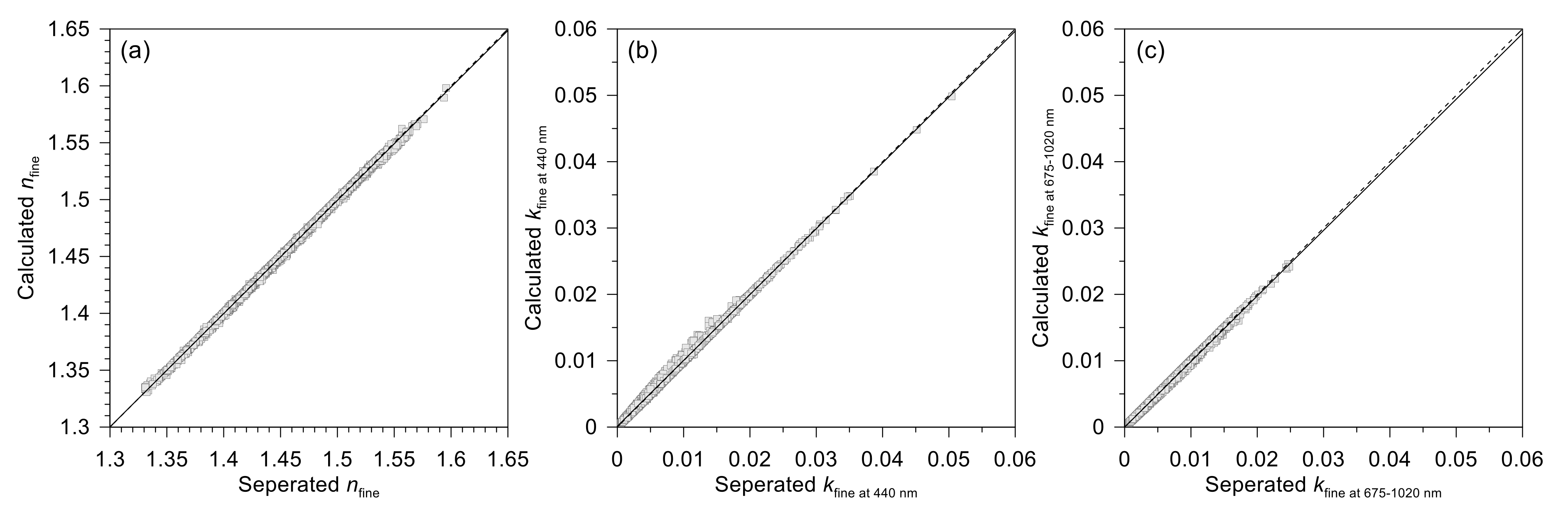
where ρ_j and V_fine are the density of jth chemical components and the volume concentration for fine-mode aerosols. Among the minimized data, we rejected the case that exceeded the χ² outlier using first and third quartiles (Q₁ and Q₃, respectively), 1.5 × [Q₃ − Q₁] + Q₃ (~6 × 10⁻³), to reduce the uncertainty from our estimation method. As a result, the total number of hourly data points was 4930 using AERONET L2* products, but this number of data reduced to 3637 (74%) when only data smaller than the χ² outlier were used. The estimated fine-mode n and k were well correlated with those separated from AERONET data, indicating that the estimated chemical components were plausible (Figure 3). The reported total relative error of BC was lowest among the other chemical components, implying that the BC estimation method used in this study should be reasonable [82].

2.5. In-Situ BC Measurements and Meteorological Data

To compare the estimated columnar BC concentration from the columnar aerosols, we used in-situ BC concentrations from co-located (or nearest) and well-validated instruments, including OC– elemental carbon (EC) analyzers (Sunset Laboratory Inc., Tigard, OR, USA) with optical corrections, multi-angle absorption photometer (MAAP 5012, Thermo Scientific), an aethalometer (AE31, Magee), and a continuous light absorption photometer (CLAP), yielding good agreement in the BC concentrations among the instruments (uncertainty ≤ ±15% except for CLAP ≤ ±20%) [12,83,84]. Hourly PM_2.5 EC was measured with a Sunset OC–EC analyzer with optical correction for Baengnyeong and Seoul. It should be noted that the BC concentration for Seoul was measured at an intensive measurement station (126.93° E, 37.61° N, 67 m asl) that is about 5.6 km northwest of the study site. A MAAP was used to measure the hourly BC in PM_2.5 at Yongin, applying an improved mass absorption efficiency (MAE) of 10.3 m² g⁻¹ instead of the default value (6.6 m² g⁻¹). This value was suggested based on calibrations using the thermal/optical method and the laser-induced incandescence technique [13,84]. The BC at Anmyon and Gosan was measured with the CLAP with a PM₁ inlet and the AE31 with a PM₁₀ inlet, respectively. The BC data from these two sites were ‘quality assessed level 2 data’ and were obtained from the European Monitoring and Evaluation Programme and the World Data Centre for Aerosols database (http://ebas.nilu.no, last accessed: 10 December 2018). We decided to ignore the uncertainty caused by the different PM inlets for the two sites because BC particles mainly exist in amounts less than 1 μm [2,85,86]. The CLAP data also showed a good correlation with the co-located PM_2.5 EC concentrations from the Sunset EC/OC analyzer, and the best-fitted line was close to one (1.17), which was slightly lower than the reported range of uncertainty of ~25% [87].

Meteorological parameters such as temperature, relative humidity (RH), wind speed, and wind direction were obtained from the European Centre for Medium-Range Weather Forecasts (ECMWF) ReAnalysis 5 (ERA5) hourly data on single and pressure levels at a resolution of 0.25° × 0.25°. In addition, the planetary boundary layer height (PBLH) was obtained from the Hybrid Single Particle Lagrangian Integrated Trajectory (HYSPLIT) Model version 4 [88] using ERA5 as the input.

3. Results

3.1. Estimated Column Concentration of Chemical Components of Fine Mode Aerosol at AERONET Sites

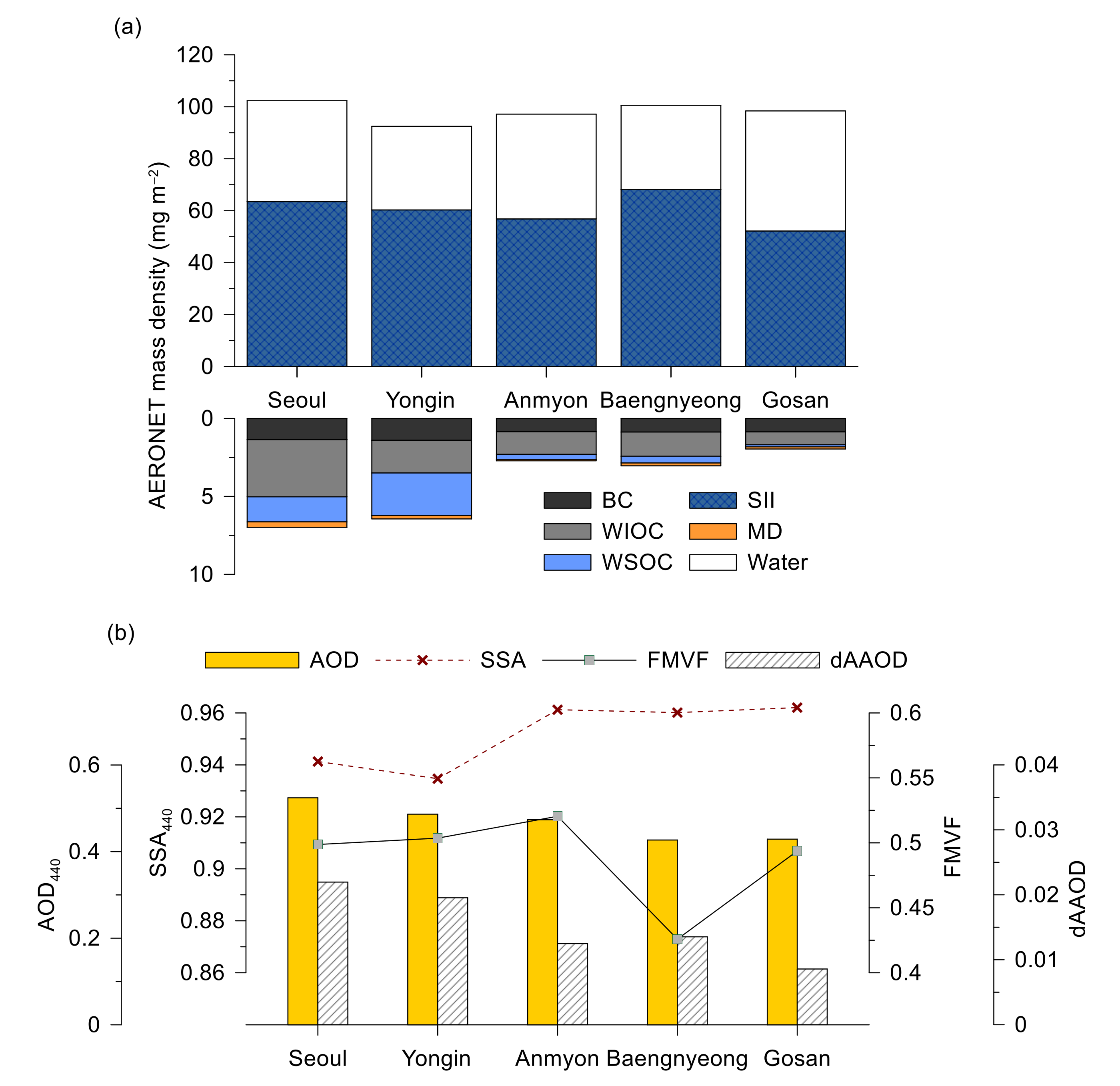
Figure 4a shows the estimated column concentration (mg m⁻²) of the considered chemical components of the fine-mode aerosols (~PM_2.5) in the columns according to site. The total column concentration was the highest in the urban region (Seoul) because of the large amount of local emissions, including those from residences and transportation. Among the chemical components, the mean with standard deviation of column concentration of SII was high, at 60.2 ± 5.5 mg m⁻², while the light-absorbing aerosols contributed minor amounts (OC [WSOC+WSIC]: 2.96 ± 1.74 mg m⁻², BC: 1.07 ± 0.25 mg m⁻², and MD: 0.20 ± 0.09 mg m⁻²). Choi and Ghim [32] reported that the mean MD and OC column concentrations (both ~10 mg m⁻²) were much higher than those from our results. Because they considered fine-mode dominant aerosols on the basis of the total RI and the measurement was conducted only in spring (March to May 2012) when MD and carbonaceous pollutants are dominant. However, previous studies in Northeast China reported the dominance of MD among the chemical components of the column concentration and volume fraction (20–80%) depending on the study period and the mixing rules because they considered both fine- and coarse-mode aerosols [28,29,30,31,33].

The variation in each chemical component showed different site dependencies. The coefficient of variation (CV; the ratio between the standard deviation and the average) of the scattering aerosols (SII and water) was very low among sites (0.09 and 0.14, respectively), whereas the light-absorbing components (BC, OC, and MD) had slightly higher CV values (0.24, 0.59, and 0.45, respectively). These results could be indicated that secondary formation was occurred uniformly over Korea, while light-absorbing aerosols were mainly influenced by local emissions. However, among the light-absorbing components, the CV of OC (especially WSOC) was higher than that of MD and BC, indicating a large spatial variability between urban/rural and background sites. In particular, the CV of WSOC (0.94) was two times higher than that of WIOC (0.50). Freshly emitted OC is primarily insoluble (WIOC), while WSOC is formed either by the chemical aging of WIOC or secondarily in the atmosphere [89]. The ratio between WSOC and OC was the highest in Yongin among the study sites, with a value of 0.56, indicating a considerable role of chemical aging and/or secondary formation in the downwind region [90]. Moreover, similar ratios that identified at Yongin were found in previous studies, with a value of 0.53 at the same location [32], 0.40–0.56 in Gwangju, Korea [91,92], and 0.51 in Beijing, China [33]. The ratio found in Seoul (0.30) was similar to reported values of 0.41 for Seoul [93] and 0.23–0.42 in Tokyo, Japan [89], but the ratio for the background sites (0.14–0.22) was slightly lower than the reported value of 0.37–0.59 in Gosan [94]. BC had the lowest CV among the light-absorbing components, with a value of 0.24, indicating relatively low spatial variation among sites, but a more detailed discussion for the variation in BC will be discussed in the next section.

The overall mean aerosol optical properties had similar characteristics to the estimated column concentration despite the aerosol optical properties representing total size aerosols, not fine-mode aerosols (Figure 4b). AOD was the highest in Seoul, with a low deviation between the sites due to the low CV of SII and water. The SSA varied according to the fraction of OC column concentration (high in Seoul and Yongin with low SSA and vice versa in other sites) along with a slightly constant BC amount. The high dAAOD in Seoul and Yongin also confirmed the high proportion of wavelength-dependent light-absorbing aerosols, especially OC, because only OC shows a spectral dependency of light absorption among the fine-mode aerosol components when considering the dominance of fine-mode aerosols (fine-mode volume fraction >~0.5).

3.2. Monthly Variation in the Columnar BC Concentration Estimated from AERONET

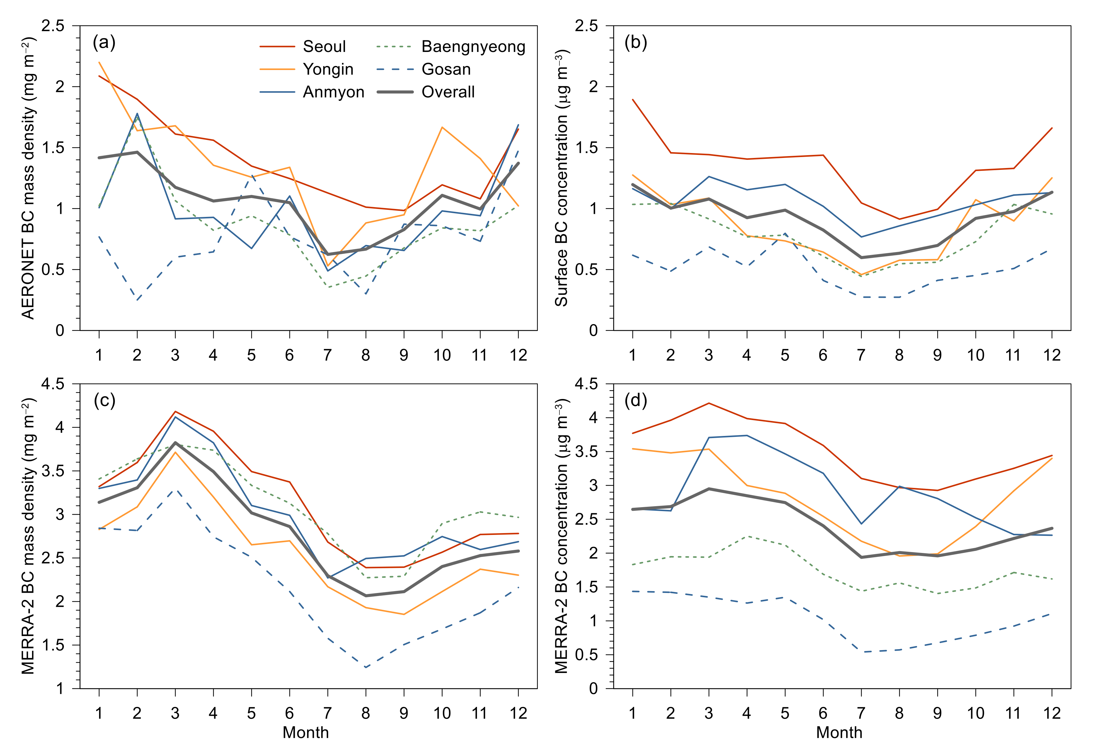
In this section, we also compared the columnar and in-situ BC concentrations from the Modern-Era Retrospective analysis for Research and Applications version 2 (MERRA-2; [95]), which is regarded as a proxy for global BC information. The mean columnar BC concentration estimated from AERONET was highest in Seoul (1.40 mg m⁻²), followed by Yongin (1.33 mg m⁻²), Anmyon (0.99 mg m⁻²), Baengnyeong (0.88 mg m⁻²), and Gosan (0.76 mg m⁻²). The columnar BC concentrations from the five sites were within a reasonable range compared to those observed in previous studies (

Table 3. Summary of comparison results between the column and the in-situ black carbon (BC) concentrations using linear regression (y = ax + b).

Study Sites	Column Concentration a	In-Situ Concentration b	R	Period	Instrument	Reference
Seoul, Korea	1.40	1.36	0.39	2011.03–2018.12	Sunset OC/EC	This study
Yongin, Korea	1.33	0.87	0.18	2015.01–2018.12	MAAP
Anmyon, Korea	0.99	1.05	0.35	2014.03–2017.04	AE31
Baengnyeong, Korea	0.88	0.78	0.48	2010.08–2016.08	Sunset OC/EC
Gosan, Korea	0.76	0.51	0.21	2012.03–2015.12	CLAP
Yongin, Korea	2.33	1.08	0.78	2012.3–2012.5	MAAP	[32]
Beijing, China	4.24	-	0.73	2014.10–2015.1 (2014.10.15–2014.11.13)	AE31	[33]
	3.70	1.44	0.79	2014.10.16–2015.1.29	AE31	[31]
	6.84	4.33	0.80	2012.10.11–2012-10.31	AE51	[29]
	-	-	0.77	2012.2.11–2.29	AE51	[28]
Cabauw, the Netherlands	0.87	0.92	0.37	2008.5.1–2008.5.15	MAAP	[71]

^a mg m⁻²; ^b μg m⁻³.

) according to the pollution levels of the sites (lower than Beijing, China, and higher than Cabauw, the Netherlands), although the previous studies did not consider only fine-mode aerosols, except for Zhang et al. [33]. However, while the in-situ BC concentrations also showed a similar order, the order of Anmyon (1.05 µg m⁻³) and Yongin (0.87 µg m⁻³) were switched. This could be partially explained by the difference in the temporal window of measurement because the in-situ measurements were conducted for 24 h regardless of the weather conditions, in contrast to the AEROENT data, which is only available for cloud-free conditions during the daytime. For this reason, the MERRA-2 BC concentrations showed a similar order to the in-situ BC concentrations, but the ranges of both column and surface concentrations from MERRA-2 were 1.9–3.6 times higher than those of the estimated column concentration from AERONET and in-situ concentration.

Figure 5a,b shows the monthly variation in the columnar BC concentration estimated from AERONET and in-situ BC concentration for each site. The overall columnar and in-situ BC concentrations began increasing in fall and peaked in winter due to house heating and/or biomass burning and were lowest in summer because of wet scavenging as a result of frequent precipitation. For each site, the monthly variation in the columnar and in-situ BC concentrations showed a slightly different pattern. In the case of Yongin, located near farmland, the columnar BC concentration was pronounced in October compared to that at the other sites. It might be attributable to biomass burning of agricultural residues, which are ubiquitous in Korea during those months [96,97]. In contrast, the columnar and in-situ BC concentrations in Gosan was the highest in May because BC might be transported from eastern China due to crop residue burning after harvest, as crop burning is prevalent in May–June rather than October–November [98].

Figure 5c,d shows the monthly variation in columnar BC and surface concentrations derived from MERRA-2. In the case of columnar BC concentration, the monthly variation among sites was more similar than that estimated from the AERONET, being the lowest in summer and the highest in spring, not in winter. Therefore, the characterized monthly variation depending on site, which was observed from AERONET and in-situ measurement (i.e., October in Yongin and May in Gosan), was diminished because MERRA-2 follows the normally well-known variations in AOD. Nevertheless, the monthly mean showed a good relationship between in-situ and surface BC concentration from MERRA-2, with high correlation coefficients (R) ranging from 0.45 (Baengnyeong) to 0.80 (Yongin). The range of R between the two datasets was similar to that found in a previous study (0.55 to 0.90) which compared 14 China Atmosphere Watch Network sites in East China during 2006–2016, and the ratio of the monthly mean between MERRA-2 and in-situ measurements (1.02 ± 0.21) showed good agreement when compared to the average value in this study (2.60 ± 0.49) [99]. The large difference in the ratio between Korea and China could be resulted from the much lower BC concentrations from MERRA-2 over Korea (less than 3.5 µg m⁻³) compared to those over East China (less than ~15 µg m⁻³).

4. Discussion

4.1. Comparison between Columnar BC Concentration Estimated from AERONET and In-Situ BC Concentrations

We compare the hourly columnar BC concentration with in-situ BC concentration. Although the PM standard was based on the daily mean to assess the short-term risk of PM, we used an hourly timescale to minimize the differences in the parameters under clear-sky conditions in the daytime and other sky conditions, which can be caused by the clear-sky bias problem [100,101]. The overall R between columnar and in-situ concentration showed a moderate value of 0.37 (p < 0.01), suggesting that the hourly relationship was highly influenced by local variabilities, such as meteorological parameters. By the sites, the highest R was observed at Baengnyeong (0.48), followed by Seoul (0.39), Anmyon (0.35), Gosan (0.21), and Yongin (0.18), indicating that the variation in in-situ BC concentration at Baengnyeong, Seoul, and Anmyon might be partially explained by the columnar BC concentration, but Gosan and Yongin are more complicated than the other sites due to other variables. These values were significantly lower than those observed in previous studies in Korea and China due to the short-term comparison periods (Table 3). Therefore, comparison with previous studies is difficult because most studies were conducted under relatively constant meteorological conditions (e.g., PBLH, temperature, and RH) and emission sources which showed high seasonal variability.

Among the R between in-situ BC concentration and the meteorological parameters, the temperature (−0.17), wind speed (−0.28), and PBLH (−0.13) were negative, whereas the columnar BC concentration and RH showed high (0.37) and low (0.06) positive correlations, respectively. As discussed in the previous section, it could be easily deduced that in-situ BC concentration was increased by low wind speeds (stagnant conditions), low PBLH (low vertical mixing), and low temperatures (high emissions from heating), resulting in accumulated BC at the surface level. The reason for the low correlation with RH is that freshly emitted BC particles have a hydrophobic property, which is less effective with RH [54]. Moreover, the growth factor of more hygroscopic BC-containing particles due to aging is generally lower than that of BC-free particles [102,103].

Table 4. Summary of statistical parameters for the relationship between the columnar and in-situ BC concentrations depending on the season and meteorological conditions. The parameters include the mean with standard deviation, correlation coefficient (R), slope, and intercept of the linear regression line (y = ax + b), and the number of data points. (a) Season, (b) wind direction, (c) wind speed, (d) relative humidity, (e) planetary boundary layer height (PBLH), and temperature.

	In-Situ Concentration (µg m−3)	Column Concentration (mg cm−2)	R	a	b	N		In-Situ Concentration (µg m−3)	Column Concentration (mg cm−2)	R	a	b	N
(a) Season							(b) Wind direction
Spring	1.40 ± 0.85	1.20 ± 0.84	0.34	0.33	0.61	1018	North	1.17 ± 0.71	1.10 ± 0.88	0.28	0.34	0.63	636
Summer	1.04 ± 0.60	0.97 ± 0.73	0.26	0.32	0.65	422	East	1.38 ± 0.86	0.92 ± 0.70	0.41	0.33	0.51	402
Fall	1.47 ± 0.90	1.05 ± 0.88	0.38	0.37	0.48	578	West	1.37 ± 0.84	1.26 ± 0.96	0.44	0.50	0.45	637
Winter	1.72 ± 1.09	1.49 ± 1.09	0.51	0.51	0.41	112	South	1.62 ± 0.99	1.17 ± 0.72	0.39	0.28	0.61	455
(c) Wind speed (m s−1)							(d) Relative humidity (%)
0–1	1.77 ± 0.98	1.18 ± 0.76	0.34	0.27	0.60	215	10–20	1.17 ± 0.60	1.53 ± 0.82	−0.23	−0.32	1.24	40
1–1.5	1.69 ± 0.90	1.29 ± 0.88	0.25	0.25	0.68	302	20–30	1.17 ± 0.72	1.40 ± 0.83	0.29	0.33	0.72	159
1.5–2	1.51 ± 0.93	1.15 ± 0.83	0.33	0.30	0.61	238	30–40	1.24 ± 0.72	1.27 ± 0.83	0.37	0.43	0.58	236
2–3	1.39 ± 0.86	1.26 ± 1.03	0.43	0.52	0.43	400	40–50	1.46 ± 0.95	1.26 ± 1.05	0.44	0.49	0.44	256
3–4	1.24 ± 0.71	1.10 ± 0.85	0.32	0.39	0.56	332	50–60	1.43 ± 0.86	1.12 ± 0.86	0.33	0.33	0.58	319
4–5	1.11 ± 0.69	1.00 ± 0.73	0.32	0.33	0.63	306	60–70	1.44 ± 0.90	1.00 ± 0.77	0.49	0.42	0.40	311
5–6	1.07 ± 0.68	0.94 ± 0.76	0.40	0.44	0.50	164	70–80	1.40 ± 0.86	1.05 ± 0.76	0.43	0.38	0.50	284
6–15	1.00 ± 0.73	0.90 ± 0.68	0.43	0.40	0.56	173	80–90	1.33 ± 0.95	0.99 ± 0.73	0.37	0.28	0.62	160
(e) PBLH (km)							(f) Temperature (°K)
0.2–0.3	1.40 ± 0.85	0.97 ± 0.73	0.35	0.30	0.57	365	263–273	1.61 ± 0.85	1.50 ± 1.02	0.50	0.60	0.35	30
0.3–0.4	1.57 ± 0.95	1.02 ± 0.70	0.40	0.30	0.55	399	273–278	1.65 ± 0.91	1.22 ± 0.88	0.46	0.45	0.40	167
0.4–0.6	1.40 ± 0.87	1.05 ± 0.78	0.45	0.41	0.46	503	278–283	1.48 ± 0.90	1.04 ± 0.73	0.41	0.33	0.53	324
0.6–0.8	1.33 ± 0.84	1.17 ± 0.90	0.39	0.42	0.53	326	283–288	1.46 ± 0.95	1.09 ± 0.78	0.32	0.27	0.65	444
0.8–1	1.19 ± 0.73	1.19 ± 0.94	0.40	0.51	0.48	231	288–293	1.33 ± 0.84	1.10 ± 0.88	0.42	0.44	0.47	466
1–1.5	1.17 ± 0.79	1.47 ± 1.07	0.51	0.69	0.45	257	293–298	1.22 ± 0.76	1.20 ± 0.97	0.41	0.53	0.46	403
1.5–2	1.12 ± 0.59	1.59 ± 0.89	−0.14	−0.21	1.14	44	298–303	1.16 ± 0.69	1.10 ± 0.76	0.25	0.27	0.71	266
2–2.5	1.23 ± 0.70	1.21 ± 0.60	0.94	0.81	0.18	5	303–313	0.99 ± 0.46	1.37 ± 1.13	0.16	0.38	0.73	29

summarizes the statistical parameters of the comparison results according to the different bins of the meteorological parameters and seasons to identify the conditions that showed a good correlation between the columnar and in-situ BC concentration. All R of the meteorological parameters and seasons were also located within significant levels. By season, the R between the hourly columnar and in-situ BC concentrations varied from 0.26 to 0.51, being high in winter and low in summer, indicating that the large variability in the BC concentration in winter resulted in a good correlation. By the same token, a high R was observed under low temperatures (263–278 °K) and relatively low RH (60–70%), which represent a typical cold season in Korea. In the case of wind direction, the west with relatively high wind speed (2–3 m s⁻¹) showed a high R because westerlies prevail on the Korean Peninsula, especially during spring and winter, resulting in a large amount of BC particles being transported from China. It should be noted that a good correlation was observed in the high planetary boundary layer (1–1.5 km) suggesting that vertical mixing is important because the columnar BC concentration represents the aerosols in the column, whereas the in-situ BC concentration is constrained under the PBLH [42].

4.2. Multiple Linear Regression (MLR) Model for Predicting Surface BC Concentration

To develop a model that can predict surface BC concentration, we used the variables discussed in the previous section in the following MLR equation [42,46], except for season which is replaced by the measurement month:

$$\begin{array}{l}B{C}_{in-situ}=C_1+C_2\cdot B{C}_{column}+C_3\cdot Temp+C_4\cdot RH+C_5\cdot PBLH\\ +C_6\cdot WS+C_7\cdot WD+C_8\cdot Month+C_9\cdot Land-usetype\end{array}$$

(7)

where BC_in-situ is in-situ BC concentration (μg m⁻³), C₁ is the intercept of the model using MLR, and C₂–C₈ are regression coefficients for the predictor variables, including the columnar BC concentration (BC_column), temperature, RH, PBLH, wind speed, wind direction, measurement month, and land-use type. The reason we replaced the season with measurement month is that measurement months showed better performance compared to season. It should be noted that the land-use type is also considered in our equation to reflect the influence of local emissions (high in urban, medium in rural, and low in background sites). The wind direction, measurement month, and land-use type parameters were considered as categorical variables and the others were continuous variables. Most estimated regression coefficients of the model were found to be highly significant (p < 0.05), except for wind directions and some measurement months (

Table 5. Estimated regression coefficients for the multiple linear regression (MLR) model.

		Coefficient
(a) Continuous variables
Intercept		−9.533 ***
BCcolumn (mg m−2)		0.330 ***
Temperature (°K)		0.022 ***
RH (%)		0.050 ***
PBLH (km)		−0.162 **
Wind speed (m s−1)		−0.041 ***
(b) Categorical variables
Wind direction	East	-
	North	0.025
	South	0.085
	West	0.043
Season	Jan	-
	Feb	0.15
	Mar	−0.212
	Apr	−0.311 *
	May	−0.574 ***
	Jun	−1.067 ***
	Jul	−1.275 ***
	Aug	−1.126 ***
	Sep	−0.935 ***
	Oct	−0.404 **
	Nov	−0.07
	Dec	0.042
Land-use	Background	-
	Rural	0.262 ***
	Urban	0.750 ***

p-value: *** p < 0.001, ** p < 0.01, * p < 0.05.

). Among the considered continuous variables, the estimated regression coefficients of temperature, PBLH, and wind speed had negative values, which is similar to the results described in Section 4.1. The columnar BC concentration and PBLH were the strongest coefficients to estimate the in-situ BC concentration. In the case of categorical variables, the urban and wintertime showed the highest coefficients suggesting the categorical variables were also followed well with already-known BC characteristics, except for the southerly wind. The difference in wind direction (not westerly wind) might be due to the considered time resolution was subdivided into months instead of seasons which can cause the weaken the wind direction effects. As a result, the coefficients of wind directions were lower than other categorical variables with insignificant levels (p ≥ 0.05).

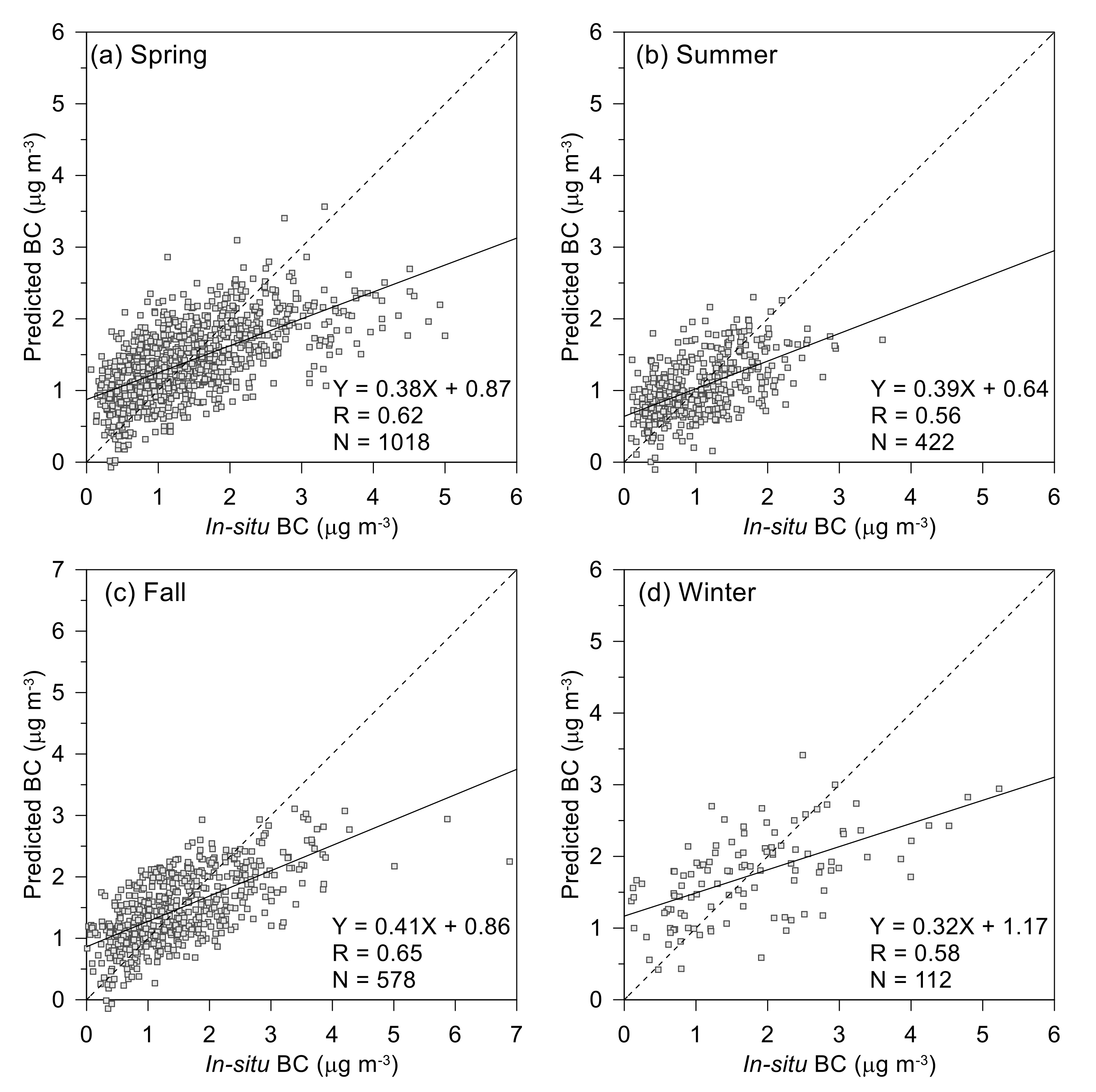
The R between in-situ and predicted BC concentrations using the MLR model was 0.64, which was much higher than the model that accounted for only the columnar BC concentration from AERONET (R = 0.37). Moreover, the slope of the linear regression line was also improved from 0.36 to 0.41 when considering the MLR model. Figure 6 presents the seasonal scatterplots between in-situ and predicted BC concentrations. The seasonal R converged into a similar range from 0.56 for summer to 0.65 for fall. Although the available number of data points in winter was significantly lower than that in other seasons, the performance in winter was comparable, yielding a higher R compared to that in summer. It should be noted that predicted BC concentrations were underestimated as in-situ concentration was increased; slopes of linear regression lines were less than unity. This could be resulted from the inherent difference in characteristics of vertical distribution between column and in-situ BC concentrations although we tried to reduce the difference by considering the PBLH, which is the indirect indicator for the vertical distribution of aerosols. The lowest slope of linear regression line in winter could be partial explained by the inherent difference in vertical distribution because the vertical mixing was restricted due to low temperature. The slope (a = 0.41) and intercept (b = 0.81) of linear regression lines might be containing the inherent difference in vertical distribution, thus, we can overcome the underestimation issue of predicted BC concentration by applying the bias correction method ([y − b]/a) using linear regression line fitting [104].

Therefore, as an aspect of R, the performance of our model can be compared with the results from previous studies that mostly focused on the relationship between the AOD and PM concentrations in Korea [46,47,105,106]. Choi et al. [105] investigated the seasonal relationship between the MODIS AOD and PM₁₀ using the 3-D global chemical transport model (GEOS-Chem) for 62 sites over East Asia. The seasonal R varied from 0.28 in fall to 0.54 in summer using linear regression methods (y = ax + b), and these values were much lower than those obtained from our model. This difference might have been due to the use of a simple linear equation and the much wider spatial distribution of monitoring sites, which showed high regional variability in meteorological parameters and emission factors. Seo et al. [46] focused on the relationship between AERONET AOD and PM₁₀ from 10 air quality monitoring stations in Seoul, Korea. They reported a much higher R value (0.68) when using an MLR model similar to our formula, but the measurement period (March to May 2012) did not cover whole seasons. Kim et al. [106] demonstrated an improved R (0.82) between AERONET AOD and PM₁₀ at Gosan for March 2008 and October 2009 using the lidar vertical fraction method, which considers the haze layer height and hygroscopic growth factor. Similarly, Kim et al. [47] also reported a high R (0.85; 0.78–0.91) between the GOCI AOD and PM_2.5 in Seoul, Korea in 2015 using the MLR model and lidar vertical profile of aerosols. On the basis of these comparisons, our model has been validated as a representative method for accurately predicting the in-situ BC concentration from AERONET sites where BC instruments are not installed, by allowing the real-time monitoring of BC during the daytime with global coverage.

5. Conclusions

Because of the increasing importance of BC emissions from developing countries and forest areas and the necessity of understanding spatial and temporal variation in BC, we investigated the columnar BC concentration from five AERONET sites in Korea using mixing rules, which can represent aerosols in the real world, and then we established an MLR model to predict the in-situ BC concentration by considering additional relevant parameters. By considering water-insoluble and water-soluble chemical components for fine-mode aerosols, the column concentrations (mg m⁻²) were estimated using (1) breakdown methods for separating the RI between fine and coarse modes and (2) mixing rules that can represent aerosols in the real world (Maxwell Garnett for water-insoluble components and volume average for water-soluble components). Among the sites, the total column concentration was associated with the geographical location; for example, it was highest in the urban area (Seoul) due to a large amount of local emissions, followed by the rural (Yongin and Anmyon) and background regions (Baengnyeong and Gosan). Among the chemical components, the mean column concentration of SII was high, at 60.2 ± 5.5 mg m⁻², with a very low CV (0.09), indicating a homogeneous distribution over Korea. In contrast, OC (2.96 ± 1.74 mg m⁻²), BC (1.07 ± 0.25 mg m⁻²), and MD (0.20 ± 0.09 mg m⁻²) had slightly higher CV values of 0.59, 0.24, and 0.45, respectively, suggesting the importance of local emissions. Among the light-absorbing components, WSOC (CV of 0.94) showed the highest spatial variation, along with WIOC (CV of 0.50), and the WSOC/OC ratio reflected site characteristics similar to those observed in previous studies. The mean columnar BC concentration was the highest and lowest in Seoul and Gosan, respectively, similar to the in-situ and MERRA-2 BC concentrations. The monthly mean columnar and in-situ BC concentrations were high in winter and spring due to house heating and/or biomass burning and the lowest in summer because of wet scavenging. The detailed monthly variation in the columnar and in-situ BC concentrations showed distinct patterns depending on the site (e.g., high values in October in Yongin and in May in Gosan due to crop residue burning), but the columnar and surface BC concentrations from the MERRA-2 reanalysis data did not show such variations and were high in spring rather than winter. When comparing the hourly in-situ BC concentration with meteorological parameters, BC increased in association with low wind speeds (stagnant conditions), low PBLH (low vertical mixing), and low temperatures (high emissions from heating), resulting in accumulated BC at the surface level. The statistical parameters for the relationship between in-situ and predicted BC concentrations using the MLR model showed similar performance (R of 0.64) to that observed in previous studies using MLR focused on the relationship between the AOD and PM concentrations in Korea (R of 0.68−0.91). Therefore, our model could be an effective tool for accurately predicting in-situ BC concentrations from AERONET data to enhance the understanding of global BC behavior.

References

- Samset, B.H.; Myhre, G.; Herber, A.; Kondo, Y.; Li, S.M.; Moteki, N.; Koike, M.; Oshima, N.; Schwarz, J.P.; Balkanski, Y.; et al. Modelled black carbon radiative forcing and atmospheric lifetime in AeroCom Phase II constrained by aircraft observations. Atmos. Chem. Phys. 2014, 14, 12465–12477. [Google Scholar] [CrossRef] [Green Version]
- Bond, T.C.; Doherty, S.J.; Fahey, D.; Forster, P.; Berntsen, T.; DeAngelo, B.; Flanner, M.; Ghan, S.; Kärcher, B.; Koch, D. Bounding the role of black carbon in the climate system: A scientific assessment. J. Geophys. Res. Atmos. 2013, 118, 5380–5552. [Google Scholar] [CrossRef]
- Geng, F.; Hua, J.; Mu, Z.; Peng, L.; Xu, X.; Chen, R.; Kan, H. Differentiating the associations of black carbon and fine particle with daily mortality in a Chinese city. Environ. Res. 2013, 120, 27–32. [Google Scholar] [CrossRef] [PubMed]
- Smith, K.R.; Jerrett, M.; Anderson, H.R.; Burnett, R.T.; Stone, V.; Derwent, R.; Atkinson, R.W.; Cohen, A.; Shonkoff, S.B.; Krewski, D.; et al. Public health benefits of strategies to reduce greenhouse-gas emissions: Health implications of short-lived greenhouse pollutants. Lancet 2009, 374, 2091–2103. [Google Scholar] [CrossRef] [Green Version]
- Suglia, S.F.; Gryparis, A.; Schwartz, J.; Wright, R.J. Association between Traffic-Related Black Carbon Exposure and Lung Function among Urban Women. Environ. Health Perspect. 2008, 116, 1333–1337. [Google Scholar] [CrossRef]
- Janssen, N.A.H.; Hoek, G.; Simic-Lawson, M.; Fischer, P.; van Bree, L.; ten Brink, H.; Keuken, M.; Atkinson Richard, W.; Anderson, H.R.; Brunekreef, B.; et al. Black Carbon as an Additional Indicator of the Adverse Health Effects of Airborne Particles Compared with PM10 and PM2.5. Environ. Health Perspect. 2011, 119, 1691–1699. [Google Scholar] [CrossRef] [Green Version]
- Loomis, D.; Grosse, Y.; Lauby-Secretan, B.; Ghissassi, F.E.; Bouvard, V.; Benbrahim-Tallaa, L.; Guha, N.; Baan, R.; Mattock, H.; Straif, K. The carcinogenicity of outdoor air pollution. The Lancet Oncol. 2013, 14, 1262–1263. [Google Scholar] [CrossRef]
- Crippa, M.; Guizzardi, D.; Muntean, M.; Schaaf, E.; Dentener, F.; van Aardenne, J.A.; Monni, S.; Doering, U.; Olivier, J.G.J.; Pagliari, V.; et al. Gridded emissions of air pollutants for the period 1970–2012 within EDGAR v4.3.2. Earth Syst. Sci. Data 2018, 10, 1987–2013. [Google Scholar] [CrossRef] [Green Version]
- Chen, X.; Wang, Z.; Yu, F.; Pan, X.; Li, J.; Ge, B.; Wang, Z.; Hu, M.; Yang, W.; Chen, H. Estimation of atmospheric aging time of black carbon particles in the polluted atmosphere over central-eastern China using microphysical process analysis in regional chemical transport model. Atmos. Environ. 2017, 163, 44–56. [Google Scholar] [CrossRef]
- Grythe, H.; Kristiansen, N.I.; Groot Zwaaftink, C.D.; Eckhardt, S.; Ström, J.; Tunved, P.; Krejci, R.; Stohl, A. A new aerosol wet removal scheme for the Lagrangian particle model FLEXPART v10. Geosci. Model Dev. 2017, 10, 1447–1466. [Google Scholar] [CrossRef] [Green Version]
- Winiger, P.; Andersson, A.; Eckhardt, S.; Stohl, A.; Gustafsson, Ö. The sources of atmospheric black carbon at a European gateway to the Arctic. Nat. Commun. 2016, 7, 12776. [Google Scholar] [CrossRef] [PubMed]
- Choi, Y.; Kanaya, Y.; Park, S.M.; Matsuki, A.; Sadanaga, Y.; Kim, S.W.; Uno, I.; Pan, X.; Lee, M.; Kim, H.; et al. Regional variability in black carbon and carbon monoxide ratio from long-term observations over East Asia: Assessment of representativeness for black carbon (BC) and carbon monoxide (CO) emission inventories. Atmos. Chem. Phys. 2020, 20, 83–98. [Google Scholar] [CrossRef] [Green Version]
- Kanaya, Y.; Pan, X.; Miyakawa, T.; Komazaki, Y.; Taketani, F.; Uno, I.; Kondo, Y. Long-term observations of black carbon mass concentrations at Fukue Island, western Japan, during 2009–2015: Constraining wet removal rates and emission strengths from East Asia. Atmos. Chem. Phys. 2016, 16, 10689–10705. [Google Scholar] [CrossRef] [Green Version]
- Choi, Y.; Ghim, Y.S.; Holben, B.N. Identification of columnar aerosol types under high aerosol optical depth conditions for a single AERONET site in Korea. J. Geophys. Res. 2016, 121, 1264–1277. [Google Scholar] [CrossRef] [Green Version]
- Russell, P.B.; Kacenelenbogen, M.; Livingston, J.M.; Hasekamp, O.P.; Burton, S.P.; Schuster, G.L.; Johnson, M.S.; Knobelspiesse, K.D.; Redemann, J.; Ramachandran, S. A multiparameter aerosol classification method and its application to retrievals from spaceborne polarimetry. J. Geophys. Res. Atmos. 2014, 119, 9838–9863. [Google Scholar] [CrossRef]
- Giles, D.M.; Holben, B.N.; Eck, T.F.; Sinyuk, A.; Smirnov, A.; Slutsker, I.; Dickerson, R.R.; Thompson, A.M.; Schafer, J.S. An analysis of AERONET aerosol absorption properties and classifications representative of aerosol source regions. J. Geophys. Res. 2012, 117, D17203. [Google Scholar] [CrossRef] [Green Version]
- Chung, C.E.; Kim, S.W.; Lee, M.; Yoon, S.C.; Lee, S. Carbonaceous aerosol AAE inferred from in-situ aerosol measurements at the Gosan ABC super site, and the implications for brown carbon aerosol. Atmos. Chem. Phys. 2012, 12, 6173–6184. [Google Scholar] [CrossRef] [Green Version]
- Bahadur, R.; Praveen, P.S.; Xu, Y.; Ramanathan, V. Solar absorption by elemental and brown carbon determined from spectral observations. Proc. Natl. Acad. Sci. USA 2012, 109, 17366–17371. [Google Scholar] [CrossRef] [Green Version]
- Kim, S.-W.; Cho, C.; Rupakheti, M. Estimating contributions of black and brown carbon to solar absorption from aethalometer and AERONET measurements in the highly polluted Kathmandu Valley, Nepal. Atmos. Res. 2021, 247, 105164. [Google Scholar] [CrossRef]
- Cho, C.; Kim, S.-W.; Lee, M.; Lim, S.; Fang, W.; Gustafsson, Ö.; Andersson, A.; Park, R.J.; Sheridan, P.J. Observation-based estimates of the mass absorption cross-section of black and brown carbon and their contribution to aerosol light absorption in East Asia. Atmos. Environ. 2019, 212, 65–74. [Google Scholar] [CrossRef]
- Schuster, G.L.; Dubovik, O.; Arola, A.; Eck, T.F.; Holben, B.N. Remote sensing of soot carbon—Part 2: Understanding the absorption Ångström exponent. Atmos. Chem. Phys. 2016, 16, 1587–1602. [Google Scholar] [CrossRef] [Green Version]
- Cazorla, A.; Bahadur, R.; Suski, K.J.; Cahill, J.F.; Chand, D.; Schmid, B.; Ramanathan, V.; Prather, K.A. Relating aerosol absorption due to soot, organic carbon, and dust to emission sources determined from in-situ chemical measurements. Atmos. Chem. Phys. 2013, 13, 9337–9350. [Google Scholar] [CrossRef] [Green Version]
- Lack, D.A.; Cappa, C.D. Impact of brown and clear carbon on light absorption enhancement, single scatter albedo and absorption wavelength dependence of black carbon. Atmos. Chem. Phys. 2010, 10, 4207–4220. [Google Scholar] [CrossRef] [Green Version]
- Arola, A.; Schuster, G.; Myhre, G.; Kazadzis, S.; Dey, S.; Tripathi, S. Inferring absorbing organic carbon content from AERONET data. Atmos. Chem. Phys. 2011, 11, 215–225. [Google Scholar] [CrossRef] [Green Version]
- Dey, S.; Tripathi, S.N.; Singh, R.P.; Holben, B.N. Retrieval of black carbon and specific absorption over Kanpur city, northern India during 2001–2003 using AERONET data. Atmos. Environ. 2006, 40, 445–456. [Google Scholar] [CrossRef]
- Schuster, G.L.; Dubovik, O.; Holben, B.N.; Clothiaux, E.E. Inferring black carbon content and specific absorption from Aerosol Robotic Network (AERONET) aerosol retrievals. J. Geophys. Res. Atmos. 2005, 110. [Google Scholar] [CrossRef]
- Arola, A.; Schuster, G.L.; Pitkänen, M.R.A.; Dubovik, O.; Kokkola, H.; Lindfors, A.V.; Mielonen, T.; Raatikainen, T.; Romakkaniemi, S.; Tripathi, S.N.; et al. Direct radiative effect by brown carbon over the Indo-Gangetic Plain. Atmos. Chem. Phys. 2015, 15, 12731–12740. [Google Scholar] [CrossRef] [Green Version]
- Li, Z.; Gu, X.; Wang, L.; Li, D.; Xie, Y.; Li, K.; Dubovik, O.; Schuster, G.; Goloub, P.; Zhang, Y.; et al. Aerosol physical and chemical properties retrieved from ground-based remote sensing measurements during heavy haze days in Beijing winter. Atmos. Chem. Phys. 2013, 13, 10171–10183. [Google Scholar] [CrossRef] [Green Version]
- Wang, L.; Li, Z.; Tian, Q.; Ma, Y.; Zhang, F.; Zhang, Y.; Li, D.; Li, K.; Li, L. Estimate of aerosol absorbing components of black carbon, brown carbon, and dust from ground-based remote sensing data of sun-sky radiometers. J. Geophys. Res. Atmos. 2013, 118, 6534–6543. [Google Scholar] [CrossRef]
- Xie, Y.; Li, Z.; Li, L.; Wang, L.; Li, D.; Chen, C.; Li, K.; Xu, H. Study on influence of different mixing rules on the aerosol components retrieval from ground-based remote sensing measurements. Atmos. Res. 2014, 145–146, 267–278. [Google Scholar] [CrossRef]
- Xie, Y.S.; Li, Z.Q.; Zhang, Y.X.; Zhang, Y.; Li, D.H.; Li, K.T.; Xu, H.; Zhang, Y.; Wang, Y.Q.; Chen, X.F.; et al. Estimation of atmospheric aerosol composition from ground-based remote sensing measurements of Sun-sky radiometer. J. Geophys. Res. Atmos. 2017, 122, 498–518. [Google Scholar] [CrossRef]
- Choi, Y.; Ghim, Y.S. Estimation of columnar concentrations of absorbing and scattering fine-mode aerosol components using AERONET data. J. Geophys. Res. 2016, 121, 13628–13640. [Google Scholar] [CrossRef]
- Zhang, Y.; Li, Z.; Sun, Y.; Lv, Y.; Xie, Y. Estimation of atmospheric columnar organic matter (OM) mass concentration from remote sensing measurements of aerosol spectral refractive indices. Atmos. Environ. 2018, 179, 107–117. [Google Scholar] [CrossRef]
- Schuster, G.L.; Dubovik, O.; Arola, A. Remote sensing of soot carbon—Part 1: Distinguishing different absorbing aerosol species. Atmos. Chem. Phys. 2016, 16, 1565–1585. [Google Scholar] [CrossRef] [Green Version]
- Al-Saadi, J.; Szykman, J.; Pierce, R.B.; Kittaka, C.; Neil, D.; Chu, D.A.; Remer, L.; Gumley, L.; Prins, E.; Weinstock, L. Improving national air quality forecasts with satellite aerosol observations. Bull. Am. Meteorol. Soc. 2005, 86, 1249–1261. [Google Scholar] [CrossRef]
- Guo, J.-P.; Zhang, X.-Y.; Che, H.-Z.; Gong, S.-L.; An, X.; Cao, C.-X.; Guang, J.; Zhang, H.; Wang, Y.-Q.; Zhang, X.-C.; et al. Correlation between PM concentrations and aerosol optical depth in eastern China. Atmos. Environ. 2009, 43, 5876–5886. [Google Scholar] [CrossRef]
- van Donkelaar, A.; Martin, R.V.; Brauer, M.; Kahn, R.; Levy, R.; Verduzco, C.; Villeneuve, P.J. Global estimates of ambient fine particulate matter concentrations from satellite-based aerosol optical depth: Development and application. Environ. Health Perspect. 2010, 118, 847. [Google Scholar] [CrossRef] [Green Version]
- Wang, J.; Christopher, S.A. Intercomparison between satellite-derived aerosol optical thickness and PM2. 5 mass: Implications for air quality studies. Geophys. Res. Lett. 2003, 30. [Google Scholar] [CrossRef]
- Chu, D.A.; Ferrare, R.; Szykman, J.; Lewis, J.; Scarino, A.; Hains, J.; Burton, S.; Chen, G.; Tsai, T.; Hostetler, C.; et al. Regional characteristics of the relationship between columnar AOD and surface PM2.5: Application of lidar aerosol extinction profiles over Baltimore–Washington Corridor during DISCOVER-AQ. Atmos. Environ. 2015, 101, 338–349. [Google Scholar] [CrossRef]
- Hoff, R.M.; Christopher, S.A. Remote sensing of particulate pollution from space: Have we reached the promised land? J. Air Waste Manag. Assoc. 2009, 59, 645–675. [Google Scholar] [CrossRef]
- Schaap, M.; Apituley, A.; Timmermans, R.M.A.; Koelemeijer, R.B.A.; de Leeuw, G. Exploring the relation between aerosol optical depth and PM2.5 at Cabauw, the Netherlands. Atmos. Chem. Phys. 2009, 9, 909–925. [Google Scholar] [CrossRef] [Green Version]
- Gupta, P.; Christopher, S.A. Particulate matter air quality assessment using integrated surface, satellite, and meteorological products: Multiple regression approach. J. Geophys. Res. Atmos. 2009, 114. [Google Scholar] [CrossRef] [Green Version]
- Hu, X.; Waller, L.A.; Lyapustin, A.; Wang, Y.; Al-Hamdan, M.Z.; Crosson, W.L.; Estes, M.G.; Estes, S.M.; Quattrochi, D.A.; Puttaswamy, S.J.; et al. Estimating ground-level PM2.5 concentrations in the Southeastern United States using MAIAC AOD retrievals and a two-stage model. Remote. Sens. Environ. 2014, 140, 220–232. [Google Scholar] [CrossRef]
- Ma, Z.; Hu, X.; Huang, L.; Bi, J.; Liu, Y. Estimating Ground-Level PM2.5 in China Using Satellite Remote Sensing. Environ. Sci. Technol. 2014, 48, 7436–7444. [Google Scholar] [CrossRef] [PubMed]
- Yao, F.; Si, M.; Li, W.; Wu, J. A multidimensional comparison between MODIS and VIIRS AOD in estimating ground-level PM2.5 concentrations over a heavily polluted region in China. Sci. Total Environ. 2018, 618, 819–828. [Google Scholar] [CrossRef] [PubMed]
- Seo, S.; Kim, J.; Lee, H.; Jeong, U.; Kim, W.; Holben, B.N.; Kim, S.W.; Song, C.H.; Lim, J.H. Estimation of PM10 concentrations over Seoul using multiple empirical models with AERONET and MODIS data collected during the DRAGON-Asia campaign. Atmos. Chem. Phys. 2015, 15, 319–334. [Google Scholar] [CrossRef] [Green Version]
- Kim, S.-M.; Yoon, J.; Moon, K.-J.; Kim, D.-R.; Koo, J.-H.; Choi, M.; Kim, K.N.; Lee, Y.G. Empirical estimation and diurnal patterns of surface PM2.5 concentration in Seoul using GOCI AOD. Korean J. Remote. Sens. 2018, 34, 451–463. [Google Scholar]
- Mok, J.; Krotkov, N.A.; Torres, O.; Jethva, H.; Li, Z.; Kim, J.; Koo, J.H.; Go, S.; Irie, H.; Labow, G.; et al. Comparisons of spectral aerosol single scattering albedo in Seoul, South Korea. Atmos. Meas. Tech. 2018, 11, 2295–2311. [Google Scholar] [CrossRef] [Green Version]
- Jung, J.; Kim, Y.J.; Lee, K.Y.; Cayetano, M.G.; Batmunkh, T.; Koo, J.H.; Kim, J. Spectral optical properties of long-range transport Asian dust and pollution aerosols over Northeast Asia in 2007 and 2008. Atmos. Chem. Phys. 2010, 10, 5391–5408. [Google Scholar] [CrossRef] [Green Version]
- Lee, Y.H.; Choi, Y.; Ghim, Y.S. Classification of diurnal patterns of particulate inorganic ions downwind of metropolitan Seoul. Environ. Sci. Pollut. Res. 2016, 23, 8917–8928. [Google Scholar] [CrossRef]
- Eck, T.F.; Holben, B.N.; Dubovik, O.; Smirnov, A.; Goloub, P.; Chen, H.B.; Chatenet, B.; Gomes, L.; Zhang, X.Y.; Tsay, S.C.; et al. Columnar aerosol optical properties at AERONET sites in central eastern Asia and aerosol transport to the tropical mid-Pacific. J. Geophys. Res. 2005, 110, D06202. [Google Scholar] [CrossRef]
- Kim, S.-W.; Yoon, S.-C.; Kim, J.; Kim, S.-Y. Seasonal and monthly variations of columnar aerosol optical properties over east Asia determined from multi-year MODIS, LIDAR, and AERONET Sun/sky radiometer measurements. Atmos. Environ. 2007, 41, 1634–1651. [Google Scholar] [CrossRef]
- Omar, A.H.; Won, J.-G.; Winker, D.M.; Yoon, S.-C.; Dubovik, O.; McCormick, M.P. Development of global aerosol models using cluster analysis of Aerosol Robotic Network (AERONET) measurements. J. Geophys. Res. 2005, 110, D10S14. [Google Scholar] [CrossRef]
- Choi, Y.; Kanaya, Y.; Takigawa, M.; Zhu, C.; Park, S.M.; Matsuki, A.; Sadanaga, Y.; Kim, S.W.; Pan, X.; Pisso, I. Investigation of the wet removal rate of black carbon in East Asia: Validation of a below- and in-cloud wet removal scheme in FLEXPART v10.4. Atmos. Chem. Phys. 2020, 1–25. [Google Scholar] [CrossRef]
- Boris, A.J.; Lee, T.; Park, T.; Choi, J.; Seo, S.J.; Collett, J.L., Jr. Fog composition at Baengnyeong Island in the eastern Yellow Sea: Detecting markers of aqueous atmospheric oxidations. Atmos. Chem. Phys. 2016, 16, 437–453. [Google Scholar] [CrossRef] [Green Version]
- Lee, T.; Choi, J.; Lee, G.; Ahn, J.; Park, J.S.; Atwood, S.A.; Schurman, M.; Choi, Y.; Chung, Y.; Collett, J.L., Jr. Characterization of aerosol composition, concentrations, and sources at Baengnyeong Island, Korea using an aerosol mass spectrometer. Atmos. Environ. 2015, 120, 297–306. [Google Scholar] [CrossRef]
- Huebert, B.J.; Bates, T.; Russell, P.B.; Shi, G.; Kim, Y.J.; Kawamura, K.; Carmichael, G.; Nakajima, T. An overview of ACE-Asia: Strategies for quantifying the relationships between Asian aerosols and their climatic impacts. J. Geophys. Res. Atmos. 2003, 108. [Google Scholar] [CrossRef] [Green Version]
- Nakajima, T.; Yoon, S.-C.; Ramanathan, V.; Shi, G.-Y.; Takemura, T.; Higurashi, A.; Takamura, T.; Aoki, K.; Sohn, B.-J.; Kim, S.-W.; et al. Overview of the Atmospheric Brown Cloud East Asian Regional Experiment 2005 and a study of the aerosol direct radiative forcing in east Asia. J. Geophys. Res. Atmos. 2007, 112. [Google Scholar] [CrossRef]
- Ramana, M.V.; Ramanathan, V.; Feng, Y.; Yoon, S.C.; Kim, S.W.; Carmichael, G.R.; Schauer, J.J. Warming influenced by the ratio of black carbon to sulphate and the black-carbon source. Nat. Geosci. 2010, 3, 542. [Google Scholar] [CrossRef]
- Holben, B.N.; Tanré, D.; Smirnov, A.; Eck, T.F.; Slutsker, I.; Abuhassan, N.; Newcomb, W.W.; Schafer, J.S.; Chatenet, B.; Lavenu, F.; et al. An emerging ground-based aerosol climatology: Aerosol optical depth from AERONET. J. Geophys. Res. 2001, 106, 12067–12097. [Google Scholar] [CrossRef]
- Holben, B.N.; Eck, T.F.; Slutsker, I.; Tanré, D.; Buis, J.P.; Setzer, A.; Vermote, E.; Reagan, J.A.; Kaufman, Y.J.; Nakajima, T.; et al. AERONET—A Federated Instrument Network and Data Archive for Aerosol Characterization. Remote Sens. Environ. 1998, 66, 1–16. [Google Scholar] [CrossRef]
- Eck, T.F.; Holben, B.N.; Reid, J.S.; Dubovik, O.; Smirnov, A.; O’Neill, N.T.; Slutsker, I.; Kinne, S. Wavelength dependence of the optical depth of biomass burning, urban, and desert dust aerosols. J. Geophys. Res. 1999, 104, 31333–31349. [Google Scholar] [CrossRef]
- Dubovik, O.; Sinyuk, A.; Lapyonok, T.; Holben, B.N.; Mishchenko, M.; Yang, P.; Eck, T.F.; Volten, H.; Muñoz, O.; Veihelmann, B.; et al. Application of spheroid models to account for aerosol particle nonsphericity in remote sensing of desert dust. J. Geophys. Res. 2006, 111, D11208. [Google Scholar] [CrossRef] [Green Version]
- Dubovik, O.; Smirnov, A.; Holben, B.N.; King, M.D.; Kaufman, Y.J.; Eck, T.F.; Slutsker, I. Accuracy assessments of aerosol optical properties retrieved from Aerosol Robotic Network (AERONET) Sun and sky radiance measurements. J. Geophys. Res. 2000, 105, 9791–9806. [Google Scholar] [CrossRef] [Green Version]
- Dubovik, O.; King, M.D. A flexible inversion algorithm for retrieval of aerosol optical properties from Sun and sky radiance measurements. J. Geophys. Res. 2000, 105, 20673–20696. [Google Scholar] [CrossRef] [Green Version]
- Eck, T.F.; Holben, B.N.; Reid, J.S.; Arola, A.; Ferrare, R.A.; Hostetler, C.A.; Crumeyrolle, S.N.; Berkoff, T.A.; Welton, E.J.; Lolli, S.; et al. Observations of rapid aerosol optical depth enhancements in the vicinity of polluted cumulus clouds. Atmos. Chem. Phys. 2014, 14, 11633–11656. [Google Scholar] [CrossRef] [Green Version]
- Giles, D.M.; Sinyuk, A.; Sorokin, M.G.; Schafer, J.S.; Smirnov, A.; Slutsker, I.; Eck, T.F.; Holben, B.N.; Lewis, J.R.; Campbell, J.R.; et al. Advancements in the Aerosol Robotic Network (AERONET) Version 3 database—Automated near-real-time quality control algorithm with improved cloud screening for Sun photometer aerosol optical depth (AOD) measurements. Atmos. Meas. Tech. 2019, 12, 169–209. [Google Scholar] [CrossRef] [Green Version]
- Sinyuk, A.; Holben, B.N.; Eck, T.F.; Giles, D.M.; Slutsker, I.; Korkin, S.; Schafer, J.S.; Smirnov, A.; Sorokin, M.; Lyapustin, A. The AERONET Version 3 aerosol retrieval algorithm, associated uncertainties and comparisons to Version 2. Atmos. Meas. Tech. Discuss. 2020, 2020, 1–80. [Google Scholar] [CrossRef]
- Schafer, J.S.; Eck, T.F.; Holben, B.N.; Thornhill, K.L.; Anderson, B.E.; Sinyuk, A.; Giles, D.M.; Winstead, E.L.; Ziemba, L.D.; Beyersdorf, A.J.; et al. Intercomparison of aerosol single-scattering albedo derived from AERONET surface radiometers and LARGE in situ aircraft profiles during the 2011 DRAGON-MD and DISCOVER-AQ experiments. J. Geophys. Res. 2014, 119, 7439–7452. [Google Scholar] [CrossRef] [Green Version]
- Andrews, E.; Ogren, J.A.; Kinne, S.; Samset, B. Comparison of AOD, AAOD and column single scattering albedo from AERONET retrievals and in situ profiling measurements. Atmos. Chem. Phys. 2017, 17, 6041–6072. [Google Scholar] [CrossRef] [Green Version]
- van Beelen, A.; Roelofs, G.; Hasekamp, O.; Henzing, J.; Röckmann, T. Estimation of aerosol water and chemical composition from AERONET Sun–sky radiometer measurements at Cabauw, the Netherlands. Atmos. Chem. Phys. 2014, 14, 5969–5987. [Google Scholar] [CrossRef] [Green Version]
- Cuesta, J.; Flamant, P.H.; Flamant, C. Synergetic technique combining elastic backscatter lidar data and sunphotometer AERONET inversion for retrieval by layer of aerosol optical and microphysical properties. Appl. Opt. 2008, 47, 4598–4611. [Google Scholar] [CrossRef] [PubMed]
- Zhang, Y.; Li, Z.; Zhang, Y.; Li, D.; Qie, L.; Che, H.; Xu, H. Estimation of aerosol complex refractive indices for both fine and coarse modes simultaneously based on AERONET remote sensing products. Atmos. Meas. Tech. 2017, 10, 3203–3213. [Google Scholar] [CrossRef] [Green Version]
- Zhu, C.; Byrd, R.H.; Lu, P.; Nocedal, J. Algorithm 778: L-BFGS-B: Fortran subroutines for large-scale bound-constrained optimization. ACM Trans. Math. Softw. 1997, 23, 550–560. [Google Scholar] [CrossRef]
- Wagner, R.; Ajtai, T.; Kandler, K.; Lieke, K.; Linke, C.; Müller, T.; Schnaiter, M.; Vragel, M. Complex refractive indices of Saharan dust samples at visible and near UV wavelengths: A laboratory study. Atmos. Chem. Phys. 2012, 12, 2491–2512. [Google Scholar] [CrossRef] [Green Version]
- Lesins, G.; Chylek, P.; Lohmann, U. A study of internal and external mixing scenarios and its effect on aerosol optical properties and direct radiative forcing. J. Geophys. Res. 2002, 107, AAC-5-1–AAC-5-12. [Google Scholar] [CrossRef]
- Bond, T.C.; Bergstrom, R.W. Light Absorption by Carbonaceous Particles: An Investigative Review. Aerosol Sci. Tech. 2006, 40, 27–67. [Google Scholar] [CrossRef]
- Kirchstetter, T.W.; Novakov, T.; Hobbs, P.V. Evidence that the spectral dependence of light absorption by aerosols is affected by organic carbon. J. Geophys. Res. 2004, 109, D21208. [Google Scholar] [CrossRef] [Green Version]
- Seinfeld, J.H.; Pandis, S.N.; Noone, K. Atmospheric chemistry and physics: From air pollution to climate change. Phys. Today 1998, 51, 88. [Google Scholar] [CrossRef]
- Klingmüller, K.; Steil, B.; Brühl, C.; Tost, H.; Lelieveld, J. Sensitivity of aerosol radiative effects to different mixing assumptions in the AEROPT 1.0 submodel of the EMAC atmospheric-chemistry–climate model. Geosci. Model Dev. 2014, 7, 2503–2516. [Google Scholar] [CrossRef] [Green Version]
- Byrd, R.H.; Lu, P.; Nocedal, J.; Zhu, C. A Limited Memory Algorithm for Bound Constrained Optimization. SIAM J. Sci. Comput. 1995, 16, 1190–1208. [Google Scholar] [CrossRef]
- Zhang, Y.; Li, Z.; Chen, Y.; de Leeuw, G.; Zhang, C.; Xie, Y.; Li, K. Improved inversion of aerosol components in the atmospheric column from remote sensing data. Atmos. Chem. Phys. 2020, 2020, 1–26. [Google Scholar] [CrossRef]
- Kanaya, Y.; Komazaki, Y.; Pochanart, P.; Liu, Y.; Akimoto, H.; Gao, J.; Wang, T.; Wang, Z. Mass concentrations of black carbon measured by four instruments in the middle of Central East China in June 2006. Atmos. Chem. Phys. 2008, 8, 7637–7649. [Google Scholar] [CrossRef] [Green Version]
- Kanaya, Y.; Taketani, F.; Komazaki, Y.; Liu, X.; Kondo, Y.; Sahu, L.K.; Irie, H.; Takashima, H. Comparison of Black Carbon Mass Concentrations Observed by Multi-Angle Absorption Photometer (MAAP) and Continuous Soot-Monitoring System (COSMOS) on Fukue Island and in Tokyo, Japan. Aerosol Sci. Technol. 2013, 47, 1–10. [Google Scholar] [CrossRef] [Green Version]
- Lim, S.; Lee, M.; Lee, G.; Kim, S.; Yoon, S.; Kang, K. Ionic and carbonaceous compositions of PM10, PM2.5 and PM1.0 at Gosan ABC Superstation and their ratios as source signature. Atmos. Chem. Phys. 2012, 12, 2007–2024. [Google Scholar] [CrossRef] [Green Version]
- Miyakawa, T.; Oshima, N.; Taketani, F.; Komazaki, Y.; Yoshino, A.; Takami, A.; Kondo, Y.; Kanaya, Y. Alteration of the size distributions and mixing states of black carbon through transport in the boundary layer in east Asia. Atmos. Chem. Phys. 2017, 17, 5851–5864. [Google Scholar] [CrossRef] [Green Version]
- Ogren, J.A.; Wendell, J.; Andrews, E.; Sheridan, P.J. Continuous light absorption photometer for long-term studies. Atmos. Meas. Tech. 2017, 10, 4805–4818. [Google Scholar] [CrossRef] [Green Version]
- Draxler, R.; Stunder, B.; Rolph, G.; Stein, A.; Taylor, A. HYSPLIT4 User’s Guide Version 4-Last Revision: February 2018. HYSPLIT Air Resources Laboratory: Silver Spring, MD, USA, 2018. Available online: https://www.arl.noaa.gov/wp_arl/wp-content/uploads/documents/reports/hysplit_user_guide.pdf (accessed on 27 November 2020).
- Kondo, Y.; Miyazaki, Y.; Takegawa, N.; Miyakawa, T.; Weber, R.J.; Jimenez, J.L.; Zhang, Q.; Worsnop, D.R. Oxygenated and water-soluble organic aerosols in Tokyo. J. Geophys. Res. Atmos. 2007, 112. [Google Scholar] [CrossRef]
- Choi, Y.; Ghim, Y.S.; Segal Rozenhaimer, M.; Redemann, J.; LeBlanc, S.E.; Lee, Y.; Lee, T.; Park, T.; Schwarz, J.P.; Lamb, K.D.; et al. Temporal and spatial variations of aerosol optical properties over the Korean peninsula during KORUS-AQ. Atmos. Environ. 2020, submitted. [Google Scholar]
- Park, S.S.; Son, S.-C. Relationship between carbonaceous components and aerosol light absorption during winter at an urban site of Gwangju, Korea. Atmos. Res. 2017, 185, 73–83. [Google Scholar] [CrossRef]
- Park, S.S.; Cho, S.Y. Tracking sources and behaviors of water-soluble organic carbon in fine particulate matter measured at an urban site in Korea. Atmos. Environ. 2011, 45, 60–72. [Google Scholar] [CrossRef]
- Choi, N.R.; Lee, J.Y.; Jung, C.H.; Lee, S.Y.; Yi, S.M.; Kim, Y.P. Concentrations and Characteristics of Carbonaceous Compounds in PM10 over Seoul : Measurement between 2006 and 2007. J. Korean Soc. Atmos. Environ. 2015, 31, 345–355. [Google Scholar] [CrossRef] [Green Version]
- Batmunkh, T.; Kim, Y.J.; Lee, K.Y.; Cayetano, M.G.; Jung, J.S.; Kim, S.Y.; Kim, K.C.; Lee, S.J.; Kim, J.S.; Chang, L.S.; et al. Time-Resolved Measurements of PM2.5 Carbonaceous Aerosols at Gosan, Korea. J. Air Waste Manag. Assoc. 2011, 61, 1174–1182. [Google Scholar] [CrossRef] [PubMed] [Green Version]
- Randles, C.A.; da Silva, A.M.; Buchard, V.; Colarco, P.R.; Darmenov, A.; Govindaraju, R.; Smirnov, A.; Holben, B.; Ferrare, R.; Hair, J.; et al. The MERRA-2 Aerosol Reanalysis, 1980 Onward. Part I: System Description and Data Assimilation Evaluation. J. Clim. 2017, 30, 6823–6850. [Google Scholar] [CrossRef] [PubMed]
- Jung, J.; Lee, S.; Kim, H.; Kim, D.; Lee, H.; Oh, S. Quantitative determination of the biomass-burning contribution to atmospheric carbonaceous aerosols in Daejeon, Korea, during the rice-harvest period. Atmos. Environ. 2014, 89, 642–650. [Google Scholar] [CrossRef]
- Ryu, S.Y.; Kim, J.E.; Zhuanshi, H.; Kim, Y.J.; Kang, G.U. Chemical Composition of Post-Harvest Biomass Burning Aerosols in Gwangju, Korea. J. Air Waste Manag. Assoc. 2004, 54, 1124–1137. [Google Scholar] [CrossRef] [PubMed]
- Li, J.; Bo, Y.; Xie, S. Estimating emissions from crop residue open burning in China based on statistics and MODIS fire products. J. Environ. Sci. 2016, 44, 158–170. [Google Scholar] [CrossRef] [PubMed]
- Xu, X.; Yang, X.; Zhu, B.; Tang, Z.; Wu, H.; Xie, L. Characteristics of MERRA-2 black carbon variation in east China during 2000–2016. Atmos. Environ. 2020, 222, 117140. [Google Scholar] [CrossRef]
- Choi, Y.; Ghim, Y.S. Assessment of the clear-sky bias issue using continuous PM10 data from two AERONET sites in Korea. J. Environ. Sci. 2017, 53, 151–160. [Google Scholar] [CrossRef]
- Christopher, S.A.; Gupta, P. Satellite Remote Sensing of Particulate Matter Air Quality: The Cloud-Cover Problem. J. Air Waste Manag. Assoc. 2010, 60, 596–602. [Google Scholar] [CrossRef]
- Ding, S.; Liu, D.; Zhao, D.; Hu, K.; Tian, P.; Zhou, W.; Huang, M.; Yang, Y.; Wang, F.; Sheng, J.; et al. Size-Related Physical Properties of Black Carbon in the Lower Atmosphere over Beijing and Europe. Environ. Sci. Technol. 2019, 53, 11112–11121. [Google Scholar] [CrossRef] [PubMed]
- Ding, S.; Zhao, D.; He, C.; Huang, M.; He, H.; Tian, P.; Liu, Q.; Bi, K.; Yu, C.; Pitt, J.; et al. Observed Interactions Between Black Carbon and Hydrometeor During Wet Scavenging in Mixed-Phase Clouds. Geophys. Res. Lett. 2019, 46, 8453–8463. [Google Scholar] [CrossRef] [Green Version]
- Ghim, Y.S.; Choi, Y.; Kim, S.; Bae, C.H.; Park, J.; Shin, H.J. Model Performance Evaluation and Bias Correction Effect Analysis for Forecasting PM2.5 Concentrations. J. Korean Soc. Atmos. Environ. 2017, 33, 11–18. [Google Scholar] [CrossRef]
- Choi, Y.-S.; Park, R.J.; Ho, C.-H. Estimates of ground-level aerosol mass concentrations using a chemical transport model with Moderate Resolution Imaging Spectroradiometer (MODIS) aerosol observations over East Asia. J. Geophys. Res. Atmos. 2009, 114. [Google Scholar] [CrossRef] [Green Version]
- Kim, K.; Lee, K.H.; Kim, J.I.; Noh, Y.; Shin, D.H.; Shin, S.K.; Lee, D.; Kim, J.; Kim, Y.J.; Song, C.H. Estimation of surface-level PM concentration from satellite observation taking into account the aerosol vertical profiles and hygroscopicity. Chemosphere 2016, 143, 32–40. [Google Scholar] [CrossRef]
Figure 1.
Locations of five selected AErosol RObotic NETwork (AERONET) sites in Korea. The background map was obtained from © Google Maps.
Figure 2.
(a) The AERONET volume size distributions and corresponding breakdown results according to fine- and coarse-mode peak fitting. Estimated wavelength-dependent complex refractive indices for both fine and coarse modes; (b) real and (c) imaginary parts. Red circles and blue squares with a solid line indicate the estimated complex refractive index for the fine and coarse modes, respectively. Open diamonds with a dotted line represent data retrieved from AERONET.
Figure 3.
Comparison of calculated and separated fine-mode refractive index from AERONET level 2* (L2*). (a) The real part (n), and the imaginary part (k) (b) at 440 nm and (c) from 675–1020 nm.
Figure 4.
(a) Estimated column concentrations of chemical components (mg m−2) depending on site. Upper and bottom figures indicate major (SII and water) and minor (BC, WIOC, WSOC, and MD) components, respectively. (b) Mean aerosol optical properties depending on site, including the aerosol optical depth (AOD), single scattering albedo (SSA), fine-mode volume fraction (FMVF), and dAAOD (AAOD at 440–1020 nm).
Figure 5.
Monthly variation in the (a) estimated AERONET columnar BC concentration (mg m−2), (b) in situ BC concentration (µg m−3). (c) and (d) MERRA-2 columnar (mg m−2) and surface BC concentration (µg m−3), respectively.
Figure 6.
Seasonal scatter plots between the predicted BC from the multiple linear regression (MLR) model and measured in-situ BC concentrations during (a) spring, (b) summer, (c) fall, and (d) winter.