Issues on the Correlation between Experimental and Numerical Results in Sheet Metal Forming Benchmarks


1
Institute of Science and Innovation in Mechanical and Industrial Engineering (INEGI), R. Dr. Roberto Frias, 400, 4200-465 Porto, Portugal
2
Department of Mechanical Engineering, Faculty of Engineering, University of Porto (FEUP), R. Dr. Roberto Frias, 4200-465 Porto, Portugal
3
CEMMPRE, Department of Mechanical Engineering, University of Coimbra, Rua Luís Reis Santos, Pinhal de Marrocos, 3030-788 Coimbra, Portugal
*
Author to whom correspondence should be addressed.
Metals 2020, 10(12), 1595; https://doi.org/10.3390/met10121595
Submission received: 23 October 2020
/
Revised: 16 November 2020
/
Accepted: 18 November 2020
/
Published: 28 November 2020
(This article belongs to the Special Issue Challenges and Achievements in Metal Forming)
Abstract
:The validation of numerical models requires the comparison between numerical and experimental results, which has led to the development of benchmark tests in order to achieve a wider participation. In the sheet metal-forming research field, the benchmarks proposed by the Numisheet conference series are a reference, because they always represented a challenge for the numerical codes within the state of the art in the modeling of sheet metal forming. From the challenges proposed along the series of Numisheet benchmarks, the springback prediction has been frequently incorporated, and is still a motivation for the development and testing of accurate modeling strategies. In fact, springback prediction poses many challenges, because it is strongly influenced by numerical parameters such as the type, order, and integration scheme of the finite elements adopted, as well as the shape and size of the finite element mesh, in addition to the constitutive model. Moreover, its measurement also requires the definition of a fixture that should not influence the actual springback and the proper definition of the measurement locations and directions. This is the subject of this contribution, which analyzes the benchmark focused on springback prediction, proposed by the Numisheet 2016 committee. Numerical results are obtained with two different codes and comparisons are performed between both numerical and experimental data. The differences between numerical results are mainly dictated by the ambiguous definition of boundary conditions. The analysis of numerical and experimental springback results should rely on the use of global planes to ensure the objectivity and simplicity in the comparison. Therefore, the analysis gives an insight into issues related to the comparison of results in complex geometries involving springback, which in turn suggests some recommendations for similar future benchmarks.
1. Introduction
In modern manufacturing industries, sheet metal-forming processes are commonly used to produce complex parts. The major concerns of the automotive industry are environmental protection (requiring low fuel consumption and low exhaust emissions) and the safety specifications [1]. Therefore, newer materials or solutions are required to reduce the weight of the vehicle body structures and closures, such as aluminum alloys and high-strength steels. The use of these materials involves a particular challenge because of their severe, and sometimes peculiar, springback behavior [2]. Additionally, meeting the dimensional specifications to produce parts made of these materials is difficult and can require expensive try-out loops. Upon completion of sheet metal forming, deep-drawn and stretch-drawn parts show high elastic recovery (springback), which thereby affects the dimensional accuracy of the finished part [3]. As a result, the manufacturing industry is faced with some practical problems: firstly, prediction of the final part geometry after springback and, secondly, appropriate tools designed to compensate for these effects.
Springback denotes the behavior of sheet metal parts to change their shape upon unloading after forming. This shape change is mainly elastically driven, since upon removal of the deformation load, a stress decrease takes place and the total strain decreases by the amount of elastic strain, which results in springback [4]. The phenomenon of springback is a major concern in the sheet metal-forming industry because it leads to assembly problems and complicates the design of the tools. Thus, prediction and compensation of springback are essential in the tool design stage, in order to adjust the variables of the forming process and achieve the dimensional requirements of the final parts.
Due to the fact that traditional trial-and-error methods for springback compensation are time-consuming, while empirical adjustments are not applicable to complex geometries, the finite element simulation of springback has become essential for tool and process design. The major advantage of the finite element method (FEM) is the possibility of modeling complicated tool geometries, while using realistic models for the material behavior [5]. In this context, the numerical codes need to be able to predict accurately the material behavior for such newer materials, which in turn needs validation of numerical results, using experimental data which include its reproducibility. The most recent models for describing the anisotropic plastic behavior of metallic sheets are reviewed in [6].
Hence, it becomes very important to correlate the numerical and experimental results of sheet metal forming. A way to achieve such reliability is to select a case study, define a standardization procedure, perform experiments, define a correct method for the measurement of selected results, and repeat the procedure in different institutions [7]. To use experimental data as a reference to validate and evaluate the accuracy of the numerical models, it may be necessary to define higher requirements for the experimental conditions (e.g., standardization of measurement methodologies, etc.) than the ones commonly adopted in industry, in order to achieve the repeatability and reproducibility of results.
The reliability of springback results depends on the intrinsic variability due to the stochastic behavior of process and material parameters [8]. The accurate prediction of springback is important to reduce scrap rates and reworks and there is a need to validate and verify those predictions with experimental results. Sometimes, validation techniques lack standardized procedures and use measurement fixtures that may impose unrealistic restraint on the part, which reduces measurement accuracy and increases the experimental error.
In this work, a Numisheet benchmark test has been studied which addresses all these concerns and compares springback predictions, obtained by different numerical simulation codes, and experimental results. In this benchmark, an aluminum AA6451-T4 blank with 3 mm thickness is stamped and trimmed before evaluating the final geometry of the obtained panel after springback. Two different models were considered using different FEM codes, AutoForm [9] and DD3IMP [1,10]. The springback results of the panel were analyzed in three different cross-sections and compared with experimental measurements from the deep-drawn part, available from the benchmark.
2. Numisheet Benchmarks
2.1. Short Historical Perspective
With the rapid increase in computation power, the finite element method (FEM) has become more attractive for analyzing and predicting forming defects, including springback. The first Numisheet Conference (defined as so, afterwards) was held in Zurich, Switzerland in 1991 [11], while the second Numisheet conference was held in Isehara, Japan in 1993. Succeeding Numisheet conferences were held in: Dearborn (USA, 1996), Besancon (France, 1999), Jeju Island (South Korea, 2002), Detroit (USA, 2005), Interlaken (Switzerland, 2008), Seoul (South Korea, 2011), Melbourne (Australia, 2014), Bristol (UK, 2016), and the most recent conference was held in Tokyo, Japan in July–August of 2018. The benchmarks proposed within this conference series and the accompanying reports [12,13,14,15,16] illustrate the state-of-the-art evolution in predicting springback with FEM [17].
The Numisheet conferences bring together experts from academia and industry for the discussion of numerical methods applied in the simulation of 3D sheet metal-forming processes. One of the most distinguishing features of the Numisheet conference series is the benchmark session, during which numerical simulations of sheet-formed parts are compared with experimental results, some of them from industry. The benchmark sessions provide an extraordinary opportunity for networking, for the exchange of technologies related to sheet metal forming and for the numerical validation of sheet metal-forming codes [14].
2.2. Numisheet 2016 Benchmark 2—Springback of an Aluminum Panel
The Numisheet conference held in Bristol, UK, in 2016, proposed three benchmarks, two of which involving the numerical simulation of industrial sheet-formed parts and the comparison with experimental results from industry. The current study deals with benchmark 2 (BM2) that focuses on the springback prediction of a complex sheet metal-formed panel, produced by Jaguar Land Rover [18]. The part consists of an aluminum panel with a maximum length of about 2000 mm, which is formed and trimmed, before being released from tools. Figure 1 shows the geometry of the die geometry (outer surface) as well as of the blank after forming and after trimming. Several trimming operations were simplified and only a global trimming line was defined, as shown in Figure 1b.
2.3. Process Conditions and Material Properties
The forming process of this benchmark includes one single forming operation followed by a trimming operation. Regarding the simulation and its correspondence to experiments or part production, several stages are considered:
- Binder closure: closing of the die-binder until attaining a fixed value for the binder force (BF);
- Forming: actual one-step forming;
- Trimming: profile trimming using a trim curve defined in the die surface;
- Springback: tool removal and measurement of defined section of final geometry, after springback.
The initial setup for the punch, die, blank holder (binder), and blank, as proposed by the Numisheet BM2 committee, is shown in Figure 2. The committee recommend a value of 0.08 for the friction coefficient between the forming tools and the blank.
The boundary conditions for the previously mentioned stages are presented in Table 1. As for the restrictions that should be applied for springback modeling, Table 2 defines the boundary conditions (BCs) for each of the three points selected, with the location shown in Figure 3. These points are also used to specify the planes for the evaluation of the part section profiles. The three planes are shown in Figure 4 and their normal vectors are presented in Table 3.
Each participant on this benchmark had to provide the numerical results for: (i) the punch force evolution with the die stroke; (ii) the thickness distribution after forming, for the three sections; and (iii) the three section profiles, for the punch-side surface, at two instants (end of forming and after trimming and springback). Regarding the punch force evolution with the die stroke, globally, the collected results shown a quite similar trend between all participants, with larger differences at the end of the die stroke. There were some technical issues with the experimental evaluation of the thickness distributions, which preclude any discussion. Nevertheless, the collection of the section profiles from each participant gave rise to the discussion on some important details, which will be addressed in this work.
3. Finite Element Method Codes and Numerical Models
In this study, two finite element codes are used to perform the BM2. One code is AutoForm (R6, AutoForm Engineering GmbH, Wilen bei Wollerau, Switzerland) [9], whose results will be labeled as AF-UP, and the other code is DD3IMP (v1.8, CEMMPRE, Coimbra, Portugal) [1,10], whose results are labeled as DD3-UC.
3.1. Finite Element Code AutoForm (AF-UP)
AutoForm is a commercial sheet metal-forming finite element code, based on the static implicit approach employing some innovative features, such as a large incremental time step under special contact treatment, an uncoupled bending–stretching solution algorithm, and adaptive mesh with increasing levels of refinement. These features, specialized for the simulations of thin sheet metal forming, render the code extremely efficient [19]. The elastic–plastic shell element considered for current analysis was element type EPS-11, i.e., eleven integration points are considered in the thickness direction [9].
3.2. In-House Finite Element Code DD3IMP (DD3-UC)
Deep-Drawing 3D Implicit code (DD3IMP) is a finite element code that has been specifically developed to simulate sheet metal-forming processes. The evolution of the deformation process is described by an updated Lagrangian scheme. An explicit approach is used to calculate an approximate first solution for the nodal displacements, the stress states, and frictional contact forces. This first trial solution is iteratively corrected, using a Newton–Raphson algorithm, finishing when a satisfactory equilibrium state in the deformable body is achieved. It is then possible to update the blank sheet configuration, as well as all the state variables, passing on to the calculation of the next time increment, and this is repeated until the end of the process. An r-min strategy is implemented to impose several restrictions on the size of the time increment in order to improve the convergence of this implicit code [10,20,21]. The numerical simulations are performed using eight-node hexahedral, tri-linear solid elements, combined with a selective reduced integration technique to avoid locking effects.
3.3. Material Models
The blank material considered is aluminum alloy (AA6451-T4) with a thickness of 3.0 mm. The benchmark committee supplied its fundamental properties, as shown in Table 4. Moreover, the uniaxial tensile yield stresses and r-values were also supplied as well as the biaxial tensile yield stress and biaxial r-values, as presented in Table 5. This enabled the participants to perform their one identification of the yield criterion parameters. Nevertheless, the participants also had access to the parameters for the Barlat’s Yld89 [22] ( = 8) yield criterion.
Regarding the hardening behavior, the benchmark committee supplied the parameters for the Voce (or Hockett/Sherby) law, describing the material behavior for the uniaxial tensile test, with the specimen oriented along the rolling direction (RD). The Voce isotropic hardening law is defined as:
where is the flow stress, is the equivalent plastic strain, and the remaining variables are material parameters; Table 6 presents their corresponding values. Moreover, the participants had access to the results from cyclical shear mechanical tests conducted (with the specimen at 0 degrees from RD) for different pre-strains, enabling the characterization of the combined isotropic/kinematic hardening (KH) behavior.
3.4. Hardening Curve
The numerical simulation AF-UP adopts the combined Swift–Hockett/Sherby isotropic hardening law:
where is the parameter controlling the combination between the two laws and the remaining variables correspond to material parameters that were identified by minimizing the squared difference to the experimental uniaxial tensile test results and are presented in Table 7.
The numerical simulation DD3-UC considers the Voce isotropic hardening law (see Equation (1)) combined with the kinematic hardening law proposed by Armstrong–Frederick:
where is back-stress tensor and its rate, is the equivalent stress, is the deviatoric component of the Cauchy stress tensor, and is the equivalent plastic strain rate. and are material parameters. Table 8 presents the parameters obtained from the best fit to the experimental data available. Figure 5 presents the evolution of the uniaxial tensile stress, predicted by both models for a specimen oriented along the rolling direction, for an equivalent plastic strain range similar to the one observed in the component.
3.5. Yield Criterion
The numerical simulation AF-UP adopts the Barlat’s Yld89 yield function [22] given by:
where and are invariants of the stress tensor defined as:
assuming the plane stress condition. is an integer exponent that is recommended to take a value of 8 for aluminum alloys. , , , and are anisotropy parameters [22]. As previously mentioned, the values for these parameters were supplied by the benchmark committee and are presented in Table 9 [18].
The numerical simulation DD3-UC adopts the Barlat’91 yield function given by:
where , , and are the principal stresses of the tensor given by:
where is the matrix of the anisotropy parameters, defined as:
where , with , are the anisotropy parameters. As for the Barlat’s Yld89, is an integer exponent and the same recommended value of 8 is considered [23]. The parameters associated with the out of plane shear stress components of this 3D yield criterion are assumed equal to the isotropic value, i.e., . The values determined for the remaining anisotropy parameters are presented in Table 10.
Figure 6 shows the comparison between the two yield surfaces in the principal stress plane as well as the evolution predicted for the r-value. The comparison with the experimental data indicates that both yield criteria enable the description of the material orthotropic behavior. Based on previous results analyzing the influence of the yield criterion on springback [24], the small differences observed are expected to have a negligible impact on the results.
4. Results of Section Profiles for the Planes Defined by Numisheet
4.1. Numisheet Published BM2 Results, after Springback
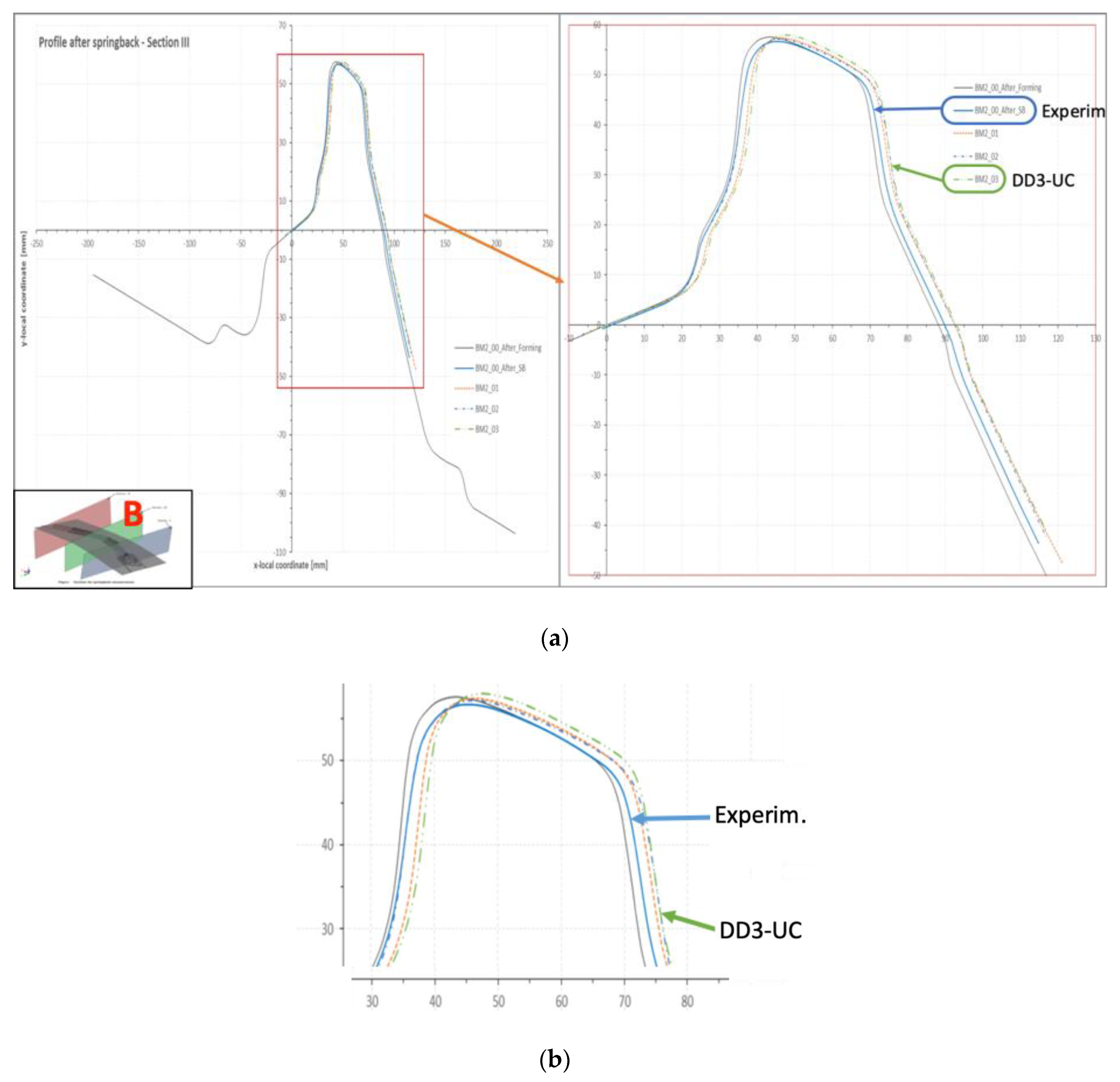
Fifteen participants from different institutions and using different codes contributed with results for benchmark 2 (BM2) of Numisheet 2016 [18]. Figure 7 and Figure 8 present the results for the profiles of sections A and B (see Section 2.3), respectively, as reported by some of the participants in this benchmark. These results correspond to the final stage “after springback” and the experimental measured data (BM2_00_After_SB) are also included for comparison. In these figures, one of the numerical participants (BM2_03 = DD3-UC) is highlighted because these results will be used in the next sections, for an improved analysis of this benchmark.
The presented section profiles are in 2D local coordinates, which means that the 3D coordinates obtained from the numerical simulation for these sections had to be transformed from the global coordinate system to the local one. The relationship between these two coordinate systems can be seen in Figure 9. The transformation and the related visualization were implemented in a MatLab script (R2018b, MathWorks, Natick, MA, USA), with the specific objective of performing this fundamental task of obtaining 2D coordinates (local frame) from 3D points (global frame).
When analyzing the results from both Figure 7 and Figure 8, for sections A and B, it is difficult to find repeatability of the numerical profiles, obtained by different participants and numerical codes. In particular, it is seen that none is following the experimental results. As previously mentioned, the participants were asked to report the same profiles at the end of the forming stage, although no experimental result was available for comparison. Since the benchmark committee supplied the IGES (Initial Graphics Exchange Specification) files for the forming tools, the profiles “after forming” were used to check the 2D transformation of the section profiles for all participants. A reference numerical result (BM2_00_After_Forming) was also plotted, as shown in Figure 7 and Figure 8. In the case of section A (Figure 7), it is observed that the numerical profiles are much closer to the experimental profile “after forming” than to the profile “after springback”, which is opposite to what would be expected. In the case of section B (Figure 8), the results show that the numerical profiles define a group which has closer results, while the experimental profile is somewhat farther away from this group. Although not presented here, the same tendency, observed in sections A and B, is found for the results of section C.
These observations were the starting point to analyze possible explanations for the divergence observed between the experimental and numerical results for this BM2 Numisheet 2016 benchmark. Note that with this kind of output (dispersion and divergence to experiments), the main objective of the benchmark, which is the validation of numerical results, is compromised. The methodology adopted to have better insight and understanding of the results was to perform the numerical simulation with AutoForm finite element (FE) code [9] and perform a detailed comparison with the results obtained using DD3IMP code [1].
4.2. Comparison of Results after Springback, AF-UP versus DD3-UC
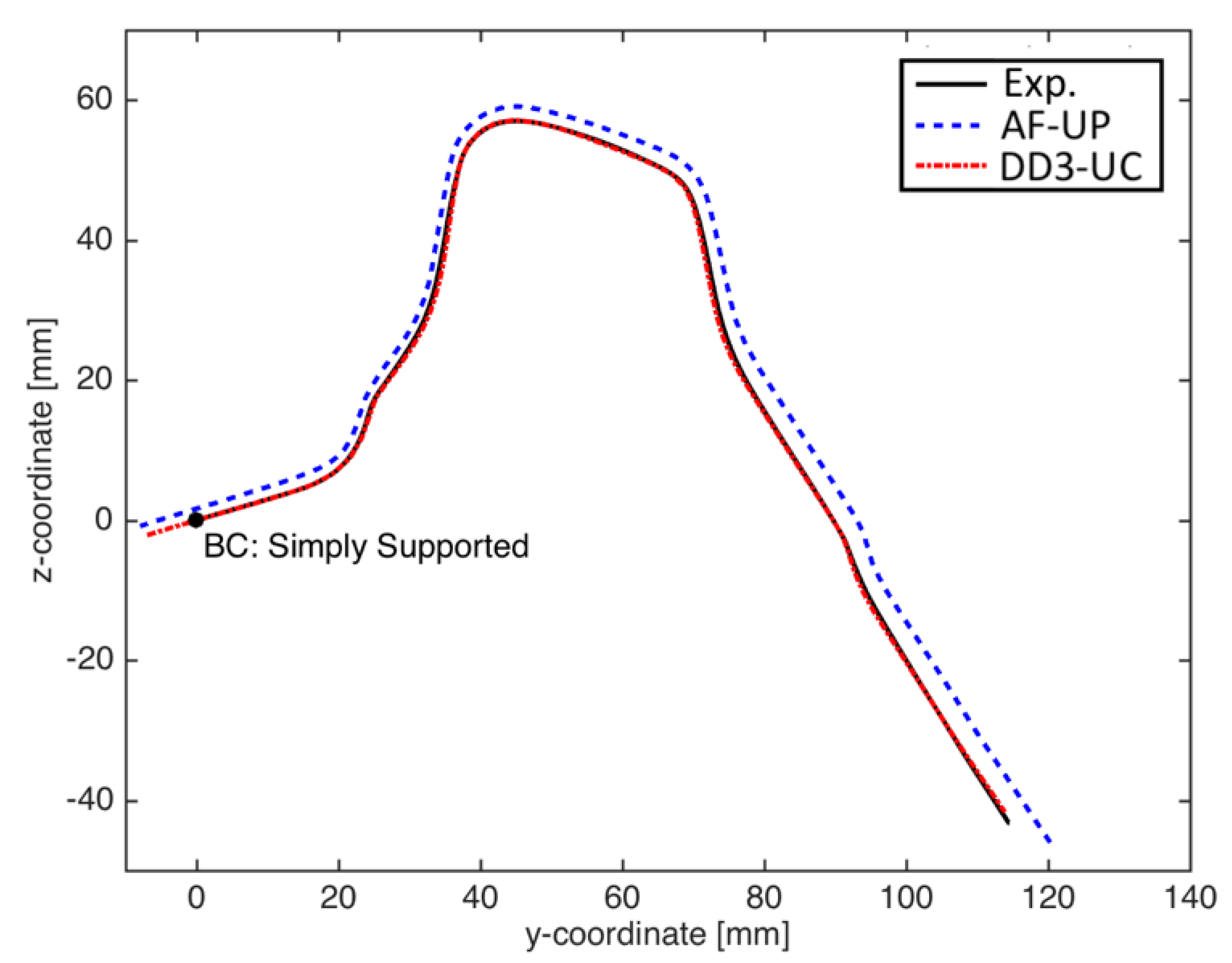
In this section, the BM2 simulation results from AutoForm code are compared with the ones obtained with DD3IMP code. The section profiles are analyzed for the proposed sections A, B, and C, i.e., they are plotted in the local 2D coordinate system. Additionally, each section was treated independently and some translations were performed, trying to guarantee the best fitting. The available 2D experimental data were also included in this comparison together with the two numerical profiles. The AF-UP results were extracted for the mid-layer of elements, while DD3-UC results use the surface in contact with the punch. Therefore, since the profile from AF-UP is always presented with an offset corresponding to half of the sheet thickness, a more efficient comparison is possible. When both profiles present a perfect match, an offset of approximately 1.5 mm will exist.
Figure 10, Figure 11 and Figure 12 show the corresponding results for sections A, B, and C, respectively. As seen in Figure 10, for section A, the numerical profiles agree closely on the right part of the profile (there is an intended offset of 1.5 mm), with both of them also following the experimental profile. On the left part of the profile, the numerical results differ and DD3-UC shows a higher springback, while the experiment is somewhat in the middle of both numerical results. An interesting observation can be seen on the top corner of the profile, which shows that the experimental profile does not match with the numerical profiles. While the numerical profiles follow a tendency of matching each other (by offset) along most of the profile, even at the top part, this is not the case for the experimental one, even at the top region. The only explanation for such behavior is that the experimental profile was not obtained for the same section or local frame of reference as the numerical ones.
By analyzing Figure 11, it is seen that the profiles agree closely; the experimental profile is coincident with DD3-UC results. AF-UP follows (with offset) the experimental results closely, but a slightly higher springback differentiates its geometry on the right side (opposite side of BC restriction). Additionally, the length of the right-side profile is different for the three profiles: AF-UP vs. DD3-UC vs. experiment. The analysis of the profiles at the end of the forming operation indicates that the material shows different flow during that stage. Nevertheless, this cannot justify the differences in length since the trimming operation should standardized the sheet dimensions. These aspects will be further analyzed in the following sections.
Figure 12 presents the results for section C, showing that AF-UP and DD3-UC numerical profiles follow each other very closely on the top surface, where the BC restriction is defined. A similar conclusion to what is observed for section A can be drawn: the right side of the numerical profiles shows a good match, while the left side shows a different springback behavior; however, again, the experimental profile does not follow the tendency of the numerical profiles, not only on the top surface, but also in the right part of profile. This reinforces the previous understanding that the cutting plane (and local coordinate system) for extracting the experimental profile is not the same as the one used for the numerical ones. This is perfectly highlighted in the detail of the top of the profile (Figure 12b), which shows a different radius of curvature for the experimental profile, when compared to the numerical ones.
4.3. Analysis of the Blank Draw-In, AF-UP versus DD3-UC
When analyzing results for a sheet stamped part, such as the geometry after springback, one should be aware that material loading history should be considered and that any difference in final results and final distribution of strains and stresses can be due to a different flow of material and loading paths. Therefore, it was decided to perform a comparison of results for the initial forming stage, including the binder closure.
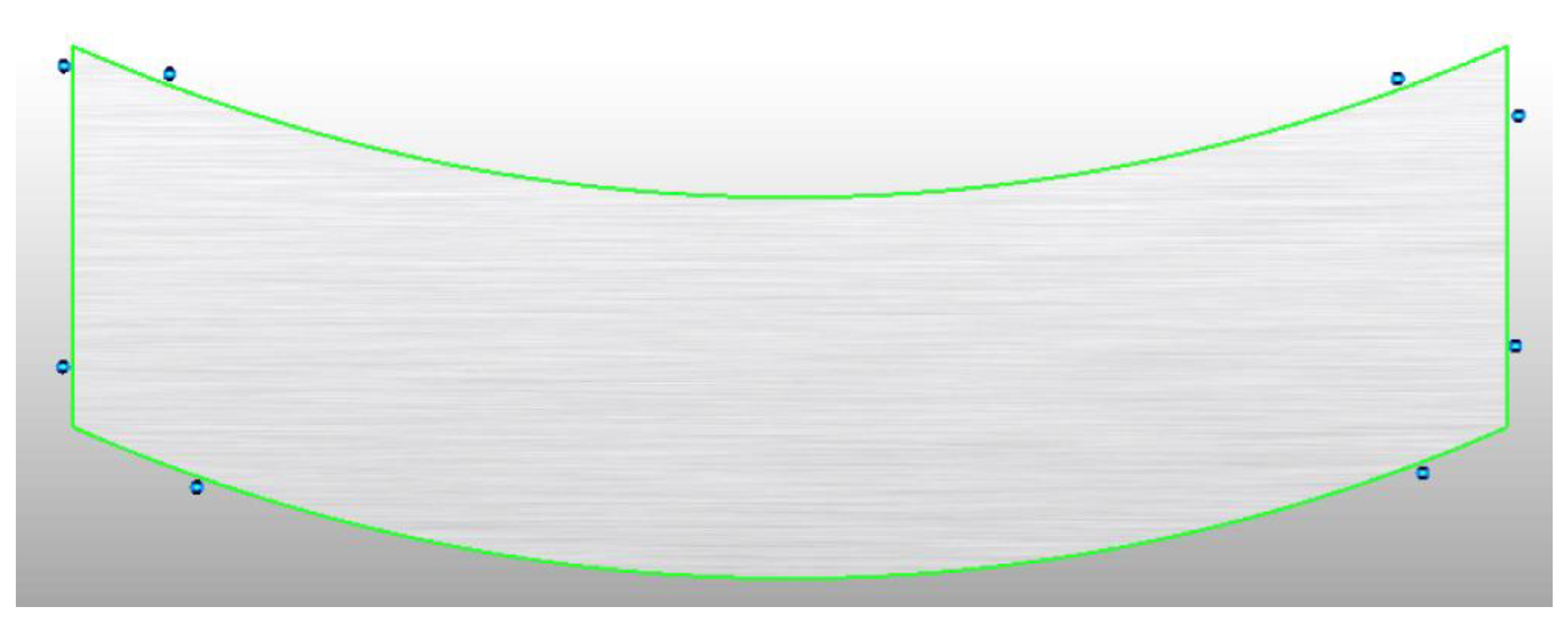
According to the process description for BM2, the blank is to be placed over the blank holder, but no information was given regarding the position of pivots to control the blank movement. In the case of the AF-UP simulation, eight pivots were defined, as shown in Figure 13. For the DD3-UC simulation, a different strategy was adopted, by restraining the movement of the nodes that establish contact with the tools, until the number of contacting nodes is sufficient to enable the removal of any additional constraints.
Figure 14 compares the initial blank position with the one after forming, enabling the evaluation of the draw-in, for AF-UP numerical results. An efficient method to compare the draw-in predicted by different codes is to use the free edges of blank and, in this case, to use the xy plane to plot the contours.
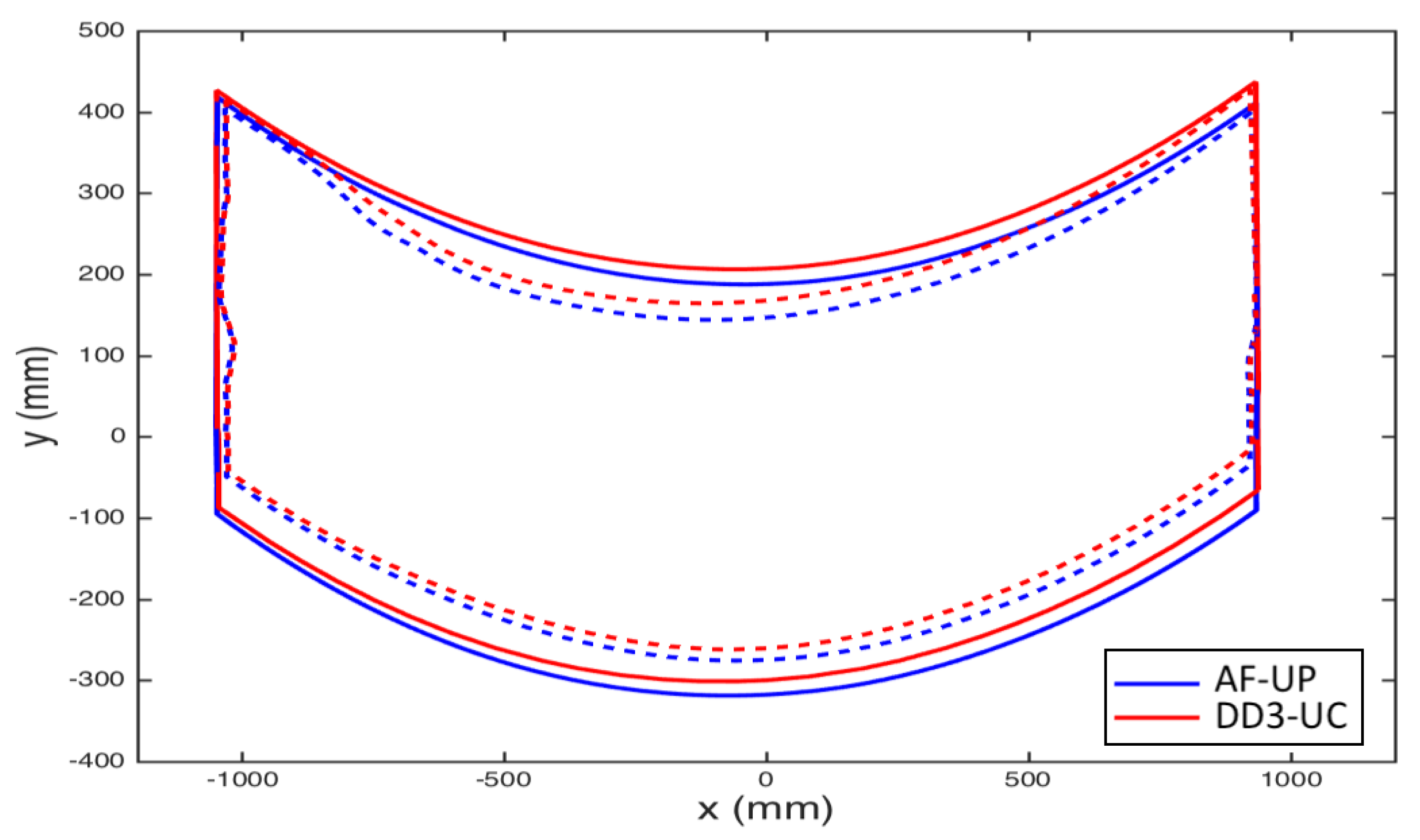
Figure 15 shows the free edges of the blanks at the end of the binder closure and after forming operations, obtained with AF-UP and DD3-UC codes. The outer boundary of the blank does not match between the two codes at the end of the binder closure. This is explained by the different strategies used to hold the blank during this operation. As a consequence, this will also give different blank positions after forming. This can be clearly seen in Figure 16, which shows the same initial blank position (Figure 16a). When the blank is held against the binder, the two blanks flow (deform) differently (see Figure 16b). Consequently, after forming (Figure 16c), the blank position keeps a difference in draw-in similar to the one observed at the end of the binder closure. This different positioning between AF-UP and DD3-UC simulations can influence the final results. A study on different benchmarks [7,25] has shown that, even for simple geometries, the different flow of the material, submitted to bending and unbending loading, causes a different loading history in some parts of the blank, which will cause visible differences in the final geometry after springback. The lack of a proper definition of the boundary conditions to be adopted in the binder closure stage is a reason for possible differences in the positioning of the blank (between benchmark participants), promoting larger differences in springback results.
4.4. Analysis of Trimming, AF-UP versus DD3-UC
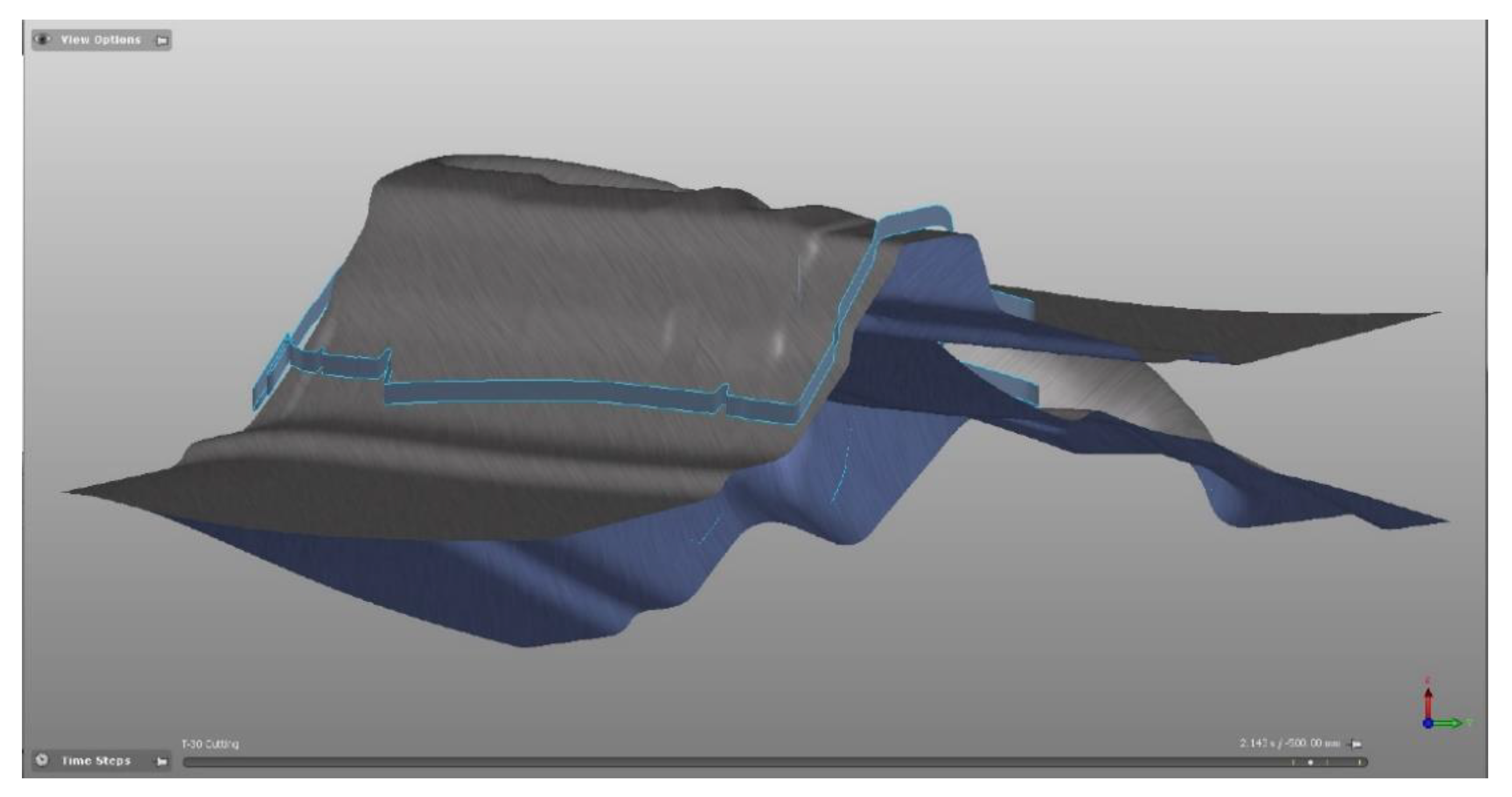
As previously mentioned, the several trimming operations were simplified and the benchmark committee supplied the global trimming line, defined over the die surface, as shown in Figure 1b. Figure 17 show the formed part, as predicted by AutoForm, as well as the trimming line (light blue). This figure highlights the distance between the trimming line and the mid-plane of the part, as well as the trimming direction selected for the AF-UP numerical simulation, which corresponds to the Oz direction in the global axes. In the DD3-UC case, since the blank is discretized with solid elements, the trimming direction was defined based on the normal to the blank surface, in order to avoid the creation of degenerated elements along the thickness direction. Figure 17 shows that in some regions of the component, the vertical and the normal directions are almost coincident, but in other zones, there are the length differences previously reported in Section 4.2. The adoption of a trimming direction normal to the blank surface will lead, in general, to a shorter length. The analysis of the results reported by other benchmark participants shows that different strategies were adopted, which can justify some of the differences in springback. The simplification of the multiple trimming operations performed in the part can be an interesting approach, to maximize the number of participants in the benchmark, but it is important to define the orientation of the trimming direction, to minimize the dispersion of the numerical results. If possible, the orientation should be taken considering the experimental operations, in order to avoid discrepancies between numerical and experimental results.
4.5. Discussion of Results
The comparison of 3D complex geometries, after springback, obtained by sheet metal forming is not a straightforward task. Even simpler to perform, the analysis of 2D geometries may lead to supplementary challenges regarding the proper comparison and repeatability of the results [7,26,27]. As shown in Figure 7 and Figure 8, for the benchmark BM2 from Numisheet 2016, the comparison between numerical and experiment results disables the extraction of definite conclusions on the capabilities of numerical predictions and for the validation of specific numerical approaches, since the numerical results are closer to each other than to the experimental ones. Nevertheless, it must be highlighted that FE simulation results globally present a high level of reliability, since they all predicted a similar tendency, not only among themselves but also for the experiment, for a challenging practical industrial problem with several different stages of production.
With the numerical simulations showing this level of reliability, a step forward it is to look for additional accuracy and increase the level of requirements. For attaining such objectives, the experimental results should also include an analysis of the level of dispersion and inaccuracy. The study performed in the previous sections highlight some details that contribute to differences, particularly between numerical and experimental results. The first one is related with the definition of sections and local planes (or coordinate systems) for the results analysis, which requires conversions and transformations, thus promoting a non-objective output of the measurement data and adding uncertainties to the results discussion. The second is related to the lack of information pertinent for the proper positioning of the blank, during the forming process, which can lead to different restrictions to the flow of the material, with consequences for different loading paths for some parts of the sheet and possible strain and stress distributions. Finally, the lack of information concerning the trimming direction, which can generate trimmed geometries with different dimensions, disables the comparison of the springback results.
Although being aware that other details can also contribute to a wider discussion on the dispersions observed for the results, it is suggested that future benchmarks consider the following details:
- When the forming process under analysis involves several stages, it would be important to have access to the results from each stage, in addition to the final geometry; if it is difficult to obtain experimental data after each stage, the comparison should be performed only for the numerical results, in order to improve the understanding of the final results; for example, the comparison of the profiles obtained after forming for BM2 would give the possibility of analyzing the influence of different numerical approaches on the draw-in;
- It is of primordial importance to find the simplest procedure for positioning the complex part in the right points of a support, since there is a need for reproducibility of the measurement of the experimental parts; this requires the selection of an appropriate experimental fixture; accordingly, the measurements of the numerical parts should follow the same standardized procedures;
- Measurement data and point coordinates should be defined from a unique global coordinate system, thus guaranteeing that a standard method for measurement exists and minimizing any need for conversions of transformations;
- Regarding the experimental results, the associated uncertainty should be included: how many experimental specimens have been used for measurement? What is the level of dispersion for the results? What is the uncertainty for validation? What is the accuracy of the equipment used in the measurements?
- The complex frictional behavior of lubricated surfaces can contribute to the uncertainty in the experimental measurements and for the discrepancy between numerical and experimental results. The use of advanced friction models, based on physical [28] and/or phenomenological [29] aspects, can help mitigate the latter.
In the next section, a further analysis of the results obtained with the two FE codes, AF-UP and DD3-UC, is performed in order to better explain two of the points mentioned previously, namely: the use of global planes (and global coordinates) and the comparison of results from intermediate stages.
5. Results of Section Profiles Using Global Planes
Figure 18 shows the comparison between the geometries after springback, as predicted by AutoForm (AF-UP) and DD3IMP (DD3-UC). The deformed meshes were exported using a standard file format (e.g., stl or unv) in order to analyze them in the post-processing software, NXT Defect Evaluator 5 [30]. This software allows for the definition of a reference geometry, including auxiliary points to guarantee the proper alignment of the parts. This is done by minimizing the distance between the reference and the geometry under analysis, taking into account the auxiliary point positions. The distance is calculated based on the normal of the reference surface. Therefore, the geometry selected as a reference determines the sign of the distance. For the example under analysis, no adjustment was performed, since both numerical models used the same global coordinate system and the same locations for the springback boundary conditions. The selected reference geometry was the DD3-UC, which corresponds to the surface in contact with the punch. Since the AF-UP geometry corresponds to the middle layer, the distance shown in Figure 18 is always positive. Note that, as in Section 4.2, a perfect matching corresponds to a distance of approximately 1.5 mm. Therefore, it is visible that the main differences in springback prediction occur in the center region and in the left and right edges of the part. The fact that the left edge shows the highest and lowest distance levels indicates that the parts rotated differently due to springback. This overall analysis of complex geometries permits a better understanding of the differences between the numerical predictions. In Figure 18, at the center region, a global plane (YZ plane) is also presented, which will be used for a comparison of the results in the next sections. This global YZ plane permits a direct plot of 3D coordinates of the sections, thus avoiding any transformation and/or rounding-off errors that may occur, in addition to an efficient comparison.
5.1. Section Profile before Forming (Binder Closure)
Figure 19 shows the comparison of numerical results between AF-UP and DD3-UC, after the binder closure. The different draw-in obtained with each code is visible, due to the use of different restrictions to the blank movement during this first processing stage, which is in agreement with the results presented in Figure 16b.
5.2. Section Profile after Forming
Figure 20 shows the section profiles obtained with AF-UP and DD3-UC after forming, highlighting their perfect match, since it is imposed by the geometry of tools, which was the same. The material draw-in is different in each code, reflecting a trend similar to the one observed after the binder closure, as already shown in Figure 16c.
5.3. Section Profile after Trimming and before Springback
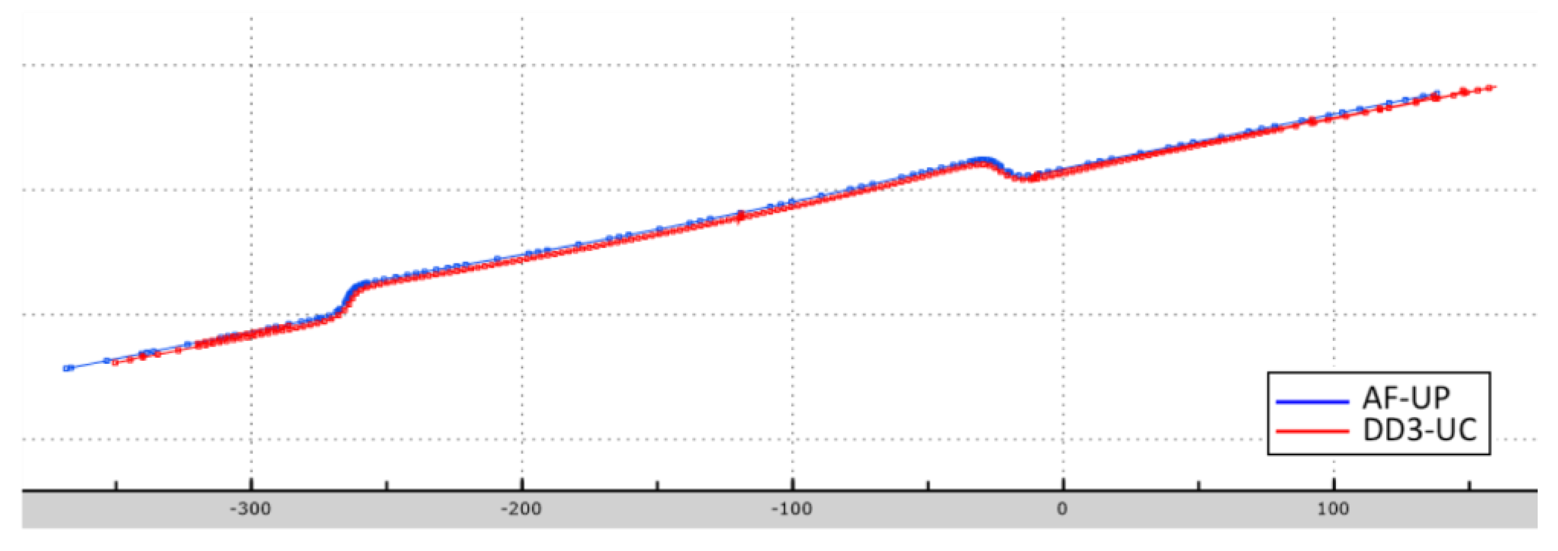
The two predicted profiles are presented in Figure 21, after the trimming stage. As for the geometries after forming, the match between the profiles is complete (imposed by the geometry of tools), except on the length. The simulation performed with AF-UP always shows a longer length because the trimming direction was considered as being coincident with the vertical one, while for DD3-UC it was defined as being equal to the normal direction to the blank surface. On the right-hand side of the part, the difference between these directions is smaller than for the left side. Since the trimming line was defined on the die surface, i.e., on a point located for a higher global coordinate Oz than the surface to be trimmed (see Figure 17), the use of a vertical trimming direction always renders a higher length for the AF-UP. This observation also agrees with the results shown in Figure 11.
5.4. Section Profile after Springback
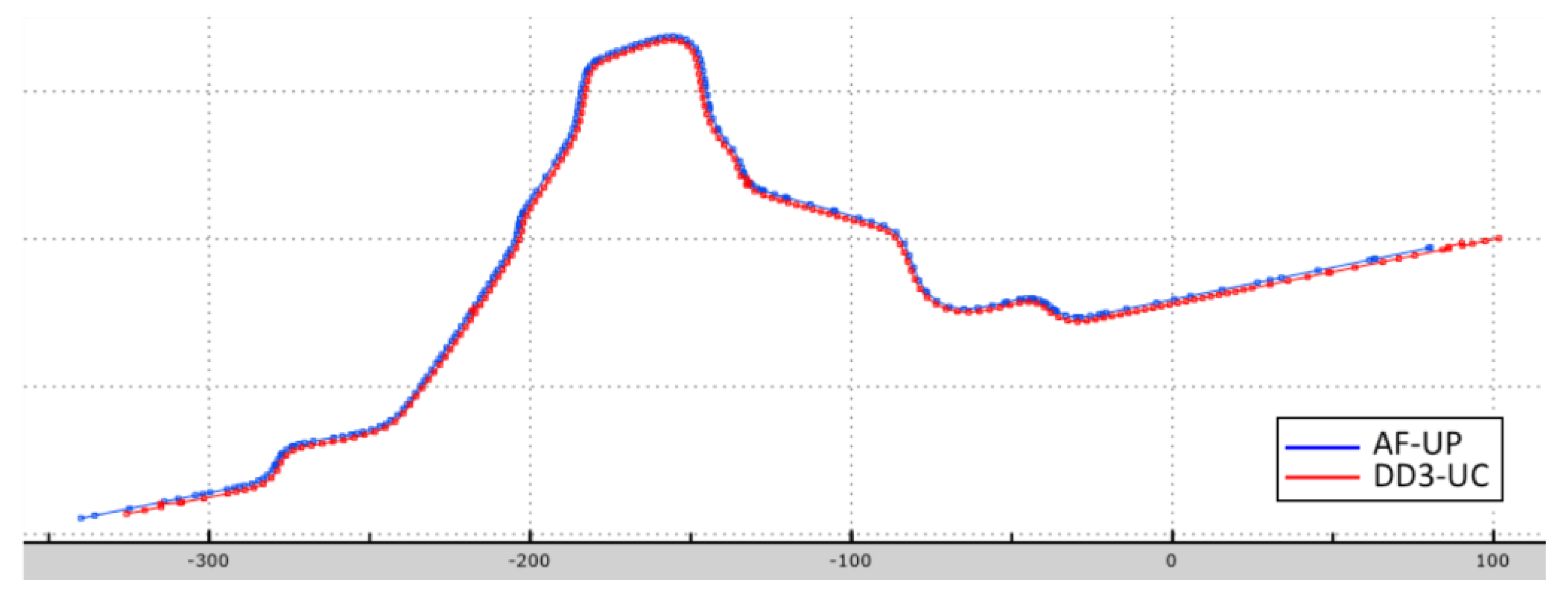
The final geometries after springback are shown in Figure 22. When comparing this figure with Figure 21, it is seen that the two profiles do not show a big springback effect, which is also in agreement to what is presented in Figure 11 (similar section, as defined in Table 2). The different trends for the opening of the part, predicted by both codes, could already be understood in Figure 18. In the center region of the part, the flange located on the upper side of the figure presents a higher positive distance (red color contour) than the lower side (green color contour), which agrees with the profiles shown in Figure 22. On the other hand, the results shown in Figure 11 present a different trend. However, in the results shown in Figure 11, each section had to be treated independently, by performing some translations. Therefore, the comparison of the results shown in Figure 11 with those of Figure 22 redirects to the difficulty of analyzing differences for complex 3D geometries and the limitations of using 2D profiles, in addition to the challenge of finding the best sections for geometry comparison after springback.
5.5. Discussion of Results
The use of global planes for comparison of results shows several advantages, such as the objectivity and simplicity in defining section profiles and corresponding measurements. Such objectivity is not only important for the comparison of numerical results, but also for assuring the correspondence with the experimental measurements, which in turn needs the definition of a simple and reliable strategy for selecting an experimental jig with a precise set of selected supporting points and frame of reference.
Having a common and solid frame of reference for experiments and numerical data, the comparison of profiles in defined planes may give the possibility of improving the results analysis, not only by enabling the qualitative study of springback, but also its quantitative study through the evaluation of the translations and rotations between profiles before and after springback.
6. Conclusions
The results from Numisheet 2016—benchmark 2 (BM2) for the final profiles after springback, obtained from benchmark participants, and the corresponding comparison with experiments, show that the comparison of complex 3D geometries is still a challenging task. The use of simple but efficient methodologies, in parallel with the best technologies for measurement and digital data comparison, seems to be best way to overcome this challenge. Advances in this topic also correspond to an important direction towards reference experimental results for validation of advanced numerical approaches, so that the needed level of accuracy is compatible with the current level of predictions from numerical FE modeling.
In this study, it was possible to understand some of the reasons that limited the conclusions extracted from Numisheet 2016—benchmark 2 (BM2), particularly because the differences between numerical and experimental results were higher than the dispersion between the numerical ones. The analysis performed gave rise to some guidelines for future benchmarks that involve the comparison of complex 3D geometries, particularly when involving multi-step processes. Recommendations to be highlighted can be summarized as follows:
- The analysis shall include the comparison of results in the main steps of the forming process, in order to improve the understanding of the final results;
- The complex part should be measured by a simple system and using well-defined points of support, so that a reliable reference system exists, ensuring an accurate comparison, both between numerical results and between numerical and experimental results;
- A unique global coordinate system shall be defined and shall represent the unique basis for measurement data and comparisons;
- Experimental results should include their associated uncertainty.
Author Contributions
Software, D.M.N., D.W., and R.L.A.; formal analysis, D.M.N., D.W., and R.L.A.; investigation, D.M.N., D.W., and R.L.A.; data curation, D.M.N., D.W., and R.L.A.; writing—original draft preparation, D.W.; writing—review and editing, A.D.S. and M.C.O.; visualization, D.M.N., D.W., and R.L.A.; supervision, A.D.S. and M.C.O. All authors have read and agreed to the published version of the manuscript.
Funding
The authors gratefully acknowledge the financial support from the Portuguese Foundation for Science and Technology (FCT) under the projects POCI-01-0145-FEDER-030592, POCI-01-0145-FEDER-032466, and NORTE-01-0145-FEDER-032419 and from UE/FEDER through the programs COMPETE 2020, NORTE 2020, CENTRO 2020 (CENTRO-01-0145-FEDER-031657), and UIDB/00285/2020.
Conflicts of Interest
The authors declare no conflict of interest. The funders had no role in the design of the study; in the collection, analyses, or interpretation of data; in the writing of the manuscript, or in the decision to publish the results.
References
- Neto, D.M.; Oliveira, M.C.; Alves, J.L.; Santos, A.D.; Menezes, L.F. Prediction of wrinkling and springback in sheet metal forming. MATEC Web Conf. 2016, 80. [Google Scholar] [CrossRef]
- Laurent, H.; Grèze, R.; Oliveira, M.C.; Menezes, L.F.; Manach, P.Y.; Alves, J.L. Numerical study of springback using the split-ring test for an AA5754 aluminum alloy. Finite Elem. Anal. Des. 2010, 46, 751–759. [Google Scholar] [CrossRef]
- Damian-Noriega, Z.; Perez-Moreno, R.; Villanueva-Pruneda, S.A.; Dominguez-Hernandez, V.M.; Puerta-Huerta, J.P.A.; Huerta-Munoz, C. A New Equation to Determine the Springback in the Bending Process of Metallic Sheet. ICCES 2008, 8, 25–30. [Google Scholar] [CrossRef]
- Vladimirov, I.N.; Pietryga, M.P.; Reese, S. Prediction of springback in sheet forming by a new finite strain model with nonlinear kinematic and isotropic hardening. J. Mater. Process. Technol. 2009, 209, 4062–4075. [Google Scholar] [CrossRef]
- Esat, V.; Darendeliler, H.; Gokler, M.I. Finite element analysis of springback in bending of aluminium sheets. Mater. Design. 2009, 23, 223–229. [Google Scholar] [CrossRef]
- Banabic, D.; Barlat, F.; Cazacu, O.; Kuwabara, T. Advances in anisotropy of plastic behaviour and formability of sheet metals. Int. J. Mater. Form. 2020, 13, 749–787. [Google Scholar] [CrossRef]
- Santos, A.D.; Teixeira, P. A study on experimental benchmarks and simulation results in sheet metal forming. J. Mater. Process. Tech. 2008, 199, 327–336. [Google Scholar] [CrossRef]
- Marretta, L.; Di Lorenzo, R. Influence of material properties variability on springback and thinning in sheet stamping processes: A stochastic analysis. Int. J. Adv. Manuf. Technol. 2010, 51, 117–134. [Google Scholar] [CrossRef]
- AutoForm-FormingSolver. Available online: https://www.autoform.com/en/ (accessed on 19 October 2020).
- Neto, D.M.; Oliveira, M.C.; Menezes, L.F.; Alves, J.L. Applying Nagata patches to smooth discretized surfaces used in 3D frictional contact problems. Comput. Method. Appl. Mech. Eng. 2014, 271, 296–320. [Google Scholar] [CrossRef]
- FE-simulation of 3D Sheet Metal Forming Processes in Automotive Industry. In Proceedings of the VDI Berichte 894, Zurich, Switzerland, 14–16 May 1991.
- Makinouchi, A.; Nakamachi, E.; Onate, E.; Wagoner, R.H. Numisheet’93. In Proceedings of the 2nd International Conference on Numerical Simulation of 3-D Sheet Metal Forming Processes; verification of simulation with experiment, Isehara, Japan, 31 August–2 September, 1993. [Google Scholar]
- Lee, J.K.; Kinzel, G.; Wagoner, R.H. Numisheet’96. In Proceedings of the 3rd International Conference: Numerical Simulation of 3-D Sheet-Metal Forming Processes: Verification of Simulations with Experiments, Detroit, MI, USA, 29 September–3 October, 1996. [Google Scholar]
- Gelin, J.C.; Picart, P. Numisheet’99. In Proceedings of the 4th International Conference and Workshop on Numerical Simulation of 3D Sheet Forming Processes, Besancon, France, 13–17 September, 1999. [Google Scholar]
- Yang, D.Y.; Oh, S.I.; Huh, H.; Kim, Y.H. Numisheet 2002. In Proceedings of the Fifth International Conference and Workshop on Numerical Simulation of 3D Sheet Forming Processes, Jeju Island, Korea, 21–25 October, 2002. [Google Scholar]
- Numisheet 2016: 10th International Conference and Workshop on Numerical Simulation of 3D Sheet Metal Forming Processes. J. Phys. 2016, 734, 011001. [CrossRef] [Green Version]
- Raabe, D.; Roters, F.; Barlat, F.; Chen, L.Q. Continuum Scale Simulation of Engineering Materials: Fundamentals-Microstructures-Process Applications; John Wiley & Sons: Hoboken, NJ, USA, 2006. [Google Scholar] [CrossRef]
- Allen, M.; Oliveira, M.C.; Hazra, S.; Adetoro, O.; Das, A.; Cardoso, R. Benchmark 2 - Springback of a Jaguar Land Rover Aluminium. J. Phys. Conf. Ser. 2016, 734, 022002. [Google Scholar] [CrossRef]
- Makinouchi, A.; Teodosiu, C.; Nakagawa, T. Advance in FEM Simulation and its Related Technologies in Sheet Metal Forming. Cirp. Ann-Manuf. Technol. 1998, 47, 641–649. [Google Scholar] [CrossRef]
- Menezes, L.; Teodosiu, C. Three-dimensional numerical simulation of the deep-drawing process using solid finite elements. J. Mater. Process. Tech. 2000, 97, 100–106. [Google Scholar] [CrossRef] [Green Version]
- Oliveira, M.C.; Alves, J.L.; Menezes, L.F. Algorithms and strategies for treatment of large deformation frictional contact in the numerical simulation of deep drawing process. Arch. Comput. Methods Eng. 2008, 15, 113–162. [Google Scholar] [CrossRef] [Green Version]
- Barlat, F.; Richmond, O. Prediction of tricomponent plane stress yield surfaces and associated flow and failure behaviour of strongly textured FCC polycrystalline sheets. Mater. Sci. Eng. 1987, 91, 15–29. [Google Scholar] [CrossRef]
- Barlat, F.; Lege, D.J.; Brem, J.C. A six-component yield function for anisotropic materials. Int. J. Plast. 1991, 7, 693–712. [Google Scholar] [CrossRef]
- Eggertsen, P.A.; Mattiasson, K. On constitutive modeling for springback analysis. Int. J. Mech. Sci. 2010, 52, 804–818. [Google Scholar] [CrossRef]
- Santos, A.D.; Ferreira Duarte, J.; Reis, A.; Barata da Rocha, A.; Menezes, L.; Oliveira, M.; Col, A.; Ono, T. Towards standard benchmarks and reference data for validation and improvement of numerical simulation in sheet metal forming. J. Mater. Process. Technol. 2002, 125, 798–805. [Google Scholar] [CrossRef] [Green Version]
- Col, A. Presentation of the 3DS research project. In Proceedings of the Fifth International Conference and Workshop on Numerical Simulation of 3D Sheet Forming Processes, Jeju Island, Korea, 21–25 October 2002; Yang, D.-Y., Oh, S.I., Huh, H., Kim, Y.H., Eds.; pp. 643–647. [Google Scholar]
- Col, A.; Santos, A.D. Influence of Stamping Rate upon Springback. In AIP Conference Proceedings; American Institute of Physics Inc.: Cambridge, MA, USA, 2005; Volume 778 A, pp. 228–233. [Google Scholar] [CrossRef]
- Hol, J.; Meinders, V.T.; deRooij, M.B.; van den Boogaard, A.H. Multi-scale friction modeling for sheet metal forming: The boundary lubrication regime. Tribol. Int. 2015, 81, 112–128. [Google Scholar] [CrossRef]
- Trzepiecinski, T.; Lemu, H.G. Recent developments and trends in the friction testing for conventional sheet metal forming and incremental sheet forming. Metals 2020, 10, 47. [Google Scholar] [CrossRef] [Green Version]
- NXT, Defect Evaluator, M&M Research, Inc. Available online: http://www.m-research.co.jp (accessed on 5 January 2020).
Figure 1.
Aluminum part from Numisheet’2016 benchmark 2; (a) outer surface of the die geometry; (b) part geometry after forming, including the trimming line; (c) final part after springback (adapted from [18]).
Figure 1.
Aluminum part from Numisheet’2016 benchmark 2; (a) outer surface of the die geometry; (b) part geometry after forming, including the trimming line; (c) final part after springback (adapted from [18]).

Figure 2.
Assembly setup for benchmark 2 of Numisheet 2016 (adapted from [16]).
Figure 2.
Assembly setup for benchmark 2 of Numisheet 2016 (adapted from [16]).

Figure 3.
Boundary conditions defined for springback modeling (adapted from [18]).
Figure 3.
Boundary conditions defined for springback modeling (adapted from [18]).

Figure 4.
Planes defining the sections for profile evaluation: (a) intersection with the formed part and (b) correspondence between the designations adopted in this work and in the benchmark (adapted from [18]).
Figure 4.
Planes defining the sections for profile evaluation: (a) intersection with the formed part and (b) correspondence between the designations adopted in this work and in the benchmark (adapted from [18]).

Figure 5.
Uniaxial tensile stress versus equivalent plastic strain, as predicted by the combined Swift–Hockett/Sherby isotropic hardening law and the Voce isotropic hardening law combined with the kinematic hardening law proposed by Armstrong–Frederick (Voce + KH).
Figure 5.
Uniaxial tensile stress versus equivalent plastic strain, as predicted by the combined Swift–Hockett/Sherby isotropic hardening law and the Voce isotropic hardening law combined with the kinematic hardening law proposed by Armstrong–Frederick (Voce + KH).

Figure 6.
Yield criteria for AA6451-T4; (a) Barlat’89 and 91 yield surfaces; (b) evolution of anisotropy with rolling direction vs. the angle from the RD.
Figure 6.
Yield criteria for AA6451-T4; (a) Barlat’89 and 91 yield surfaces; (b) evolution of anisotropy with rolling direction vs. the angle from the RD.

Figure 7.
Numisheet results—local converted 2D frame—section A, after springback: (a) as reported in [18] (adapted from [18]) and (b) detail highlighting the top region.

Figure 8.
Numisheet results—local converted 2D frame—section B, after springback: (a) as reported in [18] (adapted from [18]) and (b) detail highlighting the top region.

Figure 9.
Local converted 2D frame—section A, after springback.

Figure 10.
Section A, after springback—numerical and experimental profiles, using local 2D coordinate system; AF-UP = AutoForm code, DD3-UC = DD3IMP code; AF-UP is offset by 1.5 mm.
Figure 10.
Section A, after springback—numerical and experimental profiles, using local 2D coordinate system; AF-UP = AutoForm code, DD3-UC = DD3IMP code; AF-UP is offset by 1.5 mm.

Figure 11.
Section B, after springback—numerical and experimental profiles, using local 2D coordinate system; AF-UP = AutoForm code, DD3-UC = DD3IMP code; AF-UP is offset by 1.5 mm.
Figure 11.
Section B, after springback—numerical and experimental profiles, using local 2D coordinate system; AF-UP = AutoForm code, DD3-UC = DD3IMP code; AF-UP is offset by 1.5 mm.

Figure 12.
(a) Section C, after springback—numerical and experimental profiles, using local 2D coordinate system and (b) detail of the zone marked with the yellow rectangle in (a); AF-UP = AutoForm code, DD3-UC = DD3IMP code; AF-UP is offset by 1.5 mm.
Figure 12.
(a) Section C, after springback—numerical and experimental profiles, using local 2D coordinate system and (b) detail of the zone marked with the yellow rectangle in (a); AF-UP = AutoForm code, DD3-UC = DD3IMP code; AF-UP is offset by 1.5 mm.

Figure 13.
Blank position with pivots after binder closure in AF-UP.

Figure 14.
Blank draw-in for AF-UP simulation.

Figure 15.
Blank position before (continuous lines) and after (dashed lines) forming.

Figure 16.
Comparison of the blank contour as obtained with both codes: (a) initial position; (b) after blank holding and (c) end of forming.
Figure 16.
Comparison of the blank contour as obtained with both codes: (a) initial position; (b) after blank holding and (c) end of forming.

Figure 17.
Formed part, trimming curve defined over the die surface and trimming direction (coincident with Oz in global axis) defined in the simulation performed with AF-UP code.
Figure 17.
Formed part, trimming curve defined over the die surface and trimming direction (coincident with Oz in global axis) defined in the simulation performed with AF-UP code.

Figure 18.
AF-UP and DD3-UC predicted geometries and corresponding distance evaluation after springback (obtained using [30]).
Figure 18.
AF-UP and DD3-UC predicted geometries and corresponding distance evaluation after springback (obtained using [30]).

Figure 19.
YZ section profile after the binder closure stage; section in YZ global plane, as defined in Figure 18.
Figure 19.
YZ section profile after the binder closure stage; section in YZ global plane, as defined in Figure 18.

Figure 20.
YZ section profile after forming stage; section in YZ global plane, as defined in Figure 18.
Figure 20.
YZ section profile after forming stage; section in YZ global plane, as defined in Figure 18.

Figure 21.
YZ section profile before springback; section in YZ global plane, as defined in Figure 18.
Figure 21.
YZ section profile before springback; section in YZ global plane, as defined in Figure 18.

Figure 22.
YZ section profile after springback; section in YZ global plane, as defined in Figure 18.
Figure 22.
YZ section profile after springback; section in YZ global plane, as defined in Figure 18.


Table 1.
Boundary conditions (BCs) for forming and trimming operations.
| Part | Stage | |||
|---|---|---|---|---|
| Binder Closure | Forming | Trimming | Springback | |
| Die | Z-disp: 300 mm | Z-disp: 200 mm | - | - |
| Binder | Stopped | BF: 1900 kN | - | - |
| Blank | Free | Free | Free | apply defined BCs |
| Punch | Stopped | Stopped | - | - |
Table 2.
Boundary conditions for springback simulation.
| Point | Boundary Condition | Value |
|---|---|---|
| Point A | Pin | δx = δy = δz = 0 |
| Point B | Simply supported | δz = 0 |
| Point C | Slot | δy = δz = 0 |
Table 3.
Normal vectors for the planes defining the cross-sections for profile evaluation.
| Normal Vectors | X | Y | Z |
|---|---|---|---|
| Section A (section I) | −0.985572 | 0.100936 | −0.135870 |
| Section B (section III) | −0.997984 | −0.062806 | 0.009108 |
| Section C (section II) | −0.998390 | −0.044252 | −0.035492 |
Table 4.
Fundamental properties for AA6451-T4.
| Density, ρ (g.cm−3) | Young’s Modulus, E (GPa) | Poisson Ratio, ν |
|---|---|---|
| 2.7 | 68.9 | 0.33 |
Table 5.
Uniaxial tension and biaxial test data.
| Test Direction | Yield Stress (MPa) | r-value |
|---|---|---|
| 0° | 151.3 | 0.62 |
| 45° | 171.2 | 0.33 |
| 90° | 163.6 | 0.80 |
| Biaxial | 153.6 | 0.55 |
Table 6.
Hardening parameters for the Voce law.
| Type | A (MPa) | B (MPa) | C |
|---|---|---|---|
| Voce | 359.09 | 196.31 | 9.37 |
Table 7.
Parameters obtained for the combined Swift-Hocket/Sherby hardening law.
| α | C (MPa) | ε0 | m | σsat (MPa) | σi (MPa) | a | P |
|---|---|---|---|---|---|---|---|
| 0.5146 | 149.8 | 0.0036 | 8.78 × 10⁻⁵ | 556.6 | 175.1 | 9.376 | 1.0 |
Table 8.
Parameters obtained for the Voce isotropic hardening law combined with the Armstrong–Frederick kinematic hardening law.
Table 8.
Parameters obtained for the Voce isotropic hardening law combined with the Armstrong–Frederick kinematic hardening law.
| A (MPa) | B (MPa) | C | ||
|---|---|---|---|---|
| 340.80 | 174.11 | 11.50 | 93.89 | 48.19 |
Table 9.
Anisotropy parameters for Yld89 (m = 8.0) yield function.
| 1.3033 | 0.9556 | 0.9247 | 0.8465 |
Table 10.
Anisotropy parameters for Yld91 ( = 8.0) yield function.
| 1.0212 | 1.1936 | 0.9876 | 0.9178 |
Publisher’s Note: MDPI stays neutral with regard to jurisdictional claims in published maps and institutional affiliations. |
© 2020 by the authors. Licensee MDPI, Basel, Switzerland. This article is an open access article distributed under the terms and conditions of the Creative Commons Attribution (CC BY) license (http://creativecommons.org/licenses/by/4.0/).
Share and Cite
MDPI and ACS Style
Amaral, R.L.; Neto, D.M.; Wagre, D.; Santos, A.D.; Oliveira, M.C. Issues on the Correlation between Experimental and Numerical Results in Sheet Metal Forming Benchmarks. Metals 2020, 10, 1595. https://doi.org/10.3390/met10121595
AMA Style
Amaral RL, Neto DM, Wagre D, Santos AD, Oliveira MC. Issues on the Correlation between Experimental and Numerical Results in Sheet Metal Forming Benchmarks. Metals. 2020; 10(12):1595. https://doi.org/10.3390/met10121595
Chicago/Turabian StyleAmaral, Rui L., Diogo M. Neto, Dipak Wagre, Abel D. Santos, and Marta C. Oliveira. 2020. "Issues on the Correlation between Experimental and Numerical Results in Sheet Metal Forming Benchmarks" Metals 10, no. 12: 1595. https://doi.org/10.3390/met10121595
Note that from the first issue of 2016, this journal uses article numbers instead of page numbers. See further details here.