Hierarchical Geographic Object-Based Vegetation Type Extraction Based on Multi-Source Remote Sensing Data

1
School of Forestry, Northeast Forestry University, Harbin 150040, China
2
State Key Laboratory of Subtropical Silviculture, Zhejiang A & F University, Lin’an, Hangzhou 311300, China
*
Author to whom correspondence should be addressed.
Forests 2020, 11(12), 1271; https://doi.org/10.3390/f11121271
Submission received: 24 September 2020
/
Revised: 19 November 2020
/
Accepted: 20 November 2020
/
Published: 28 November 2020
(This article belongs to the Special Issue Monitoring and Assessing Forest Attributes Based on Remote Sensing Technology)
Abstract
:Providing vegetation type information with accurate surface distribution is one of the important tasks of remote sensing of the ecological environment. Many studies have explored ecosystem structure information at specific spatial scales based on specific remote sensing data, but it is still rare to extract vegetation information at various landscape levels from a variety of remote sensing data. Based on Gaofen-1 satellite (GF-1) Wide-Field-View (WFV) data (16 m), Ziyuan-3 satellite (ZY-3) and airborne LiDAR data, this study comparatively analyzed the four levels of vegetation information by using the geographic object-based image analysis method (GEOBIA) on the typical natural secondary forest in Northeast China. The four levels of vegetation information include vegetation/non-vegetation (L1), vegetation type (L2), forest type (L3) and canopy and canopy gap (L4). The results showed that vegetation height and density provided by airborne LiDAR data could extract vegetation features and categories more effectively than the spectral information provided by GF-1 and ZY-3 images. Only 0.5 m LiDAR data can extract four levels of vegetation information (L1–L4); and from L1 to L4, the total accuracy of the classification decreased orderly 98%, 93%, 80% and 69%. Comparing with 2.1 m ZY-3, the total classification accuracy of L1, L2 and L3 extracted by 2.1 m LiDAR data increased by 3%, 17% and 43%, respectively. At the vegetation/non-vegetation level, the spatial resolution of data plays a leading role, and the data types used at the vegetation type and forest type level become the main influencing factors. This study will provide reference for data selection and mapping strategies for hierarchical multi-scale vegetation type extraction.
1. Introduction
Providing multi-scale spatial distribution information of vegetation types plays a key role in understanding, managing and protecting vegetation ecosystems and their biodiversity. At present, remote sensing has become an important source of information for vegetation type information management and monitoring, and it is also an effective low-cost technical means for obtaining vegetation types [1,2,3]. Remote sensing technology for vegetation classification mainly includes multispectral remote sensing image classification, multi-temporal remote sensing classification, hyperspectral remote sensing classification, high spatial resolution remote sensing classification and multi-sensor remote sensing data collaborative classification [4,5,6,7]. It is necessary to study the multi-source remote sensing data to obtain the vegetation structure information of the ecosystem and the multi-scale information of the forest landscape. Since each scale corresponds to a certain ecological structure or process set, this information is closely related to the management and protection measures on the corresponding scale [8]. However, most of the research on the structure of ecosystems using remote sensing technology only explores the information on a specific single scale based on the spatial resolution of the remote sensing data used. The extraction of vegetation information at various levels of the landscape from the integrated multi-source remote sensing data is a lack of studies.
Optical data is currently the primary source of vegetation classification due to the availability of free, multi-temporal and global satellite data sets [9,10,11]. With the development of remote sensing data acquisition technology, the demand for remote sensing applications has increased, and the acquisition of high spatial resolution remote sensing data is gradually becoming more and more popular [12,13,14]. Among them, a medium-high spatial resolution (1–30 m) remote sensing image has great potential in resource environment monitoring due to its high spatial and temporal resolution and low acquisition cost [15,16]. Especially since 2012, China earthquake observation satellites such as China Gaofen-1 (GF-1) and Ziyuan-3 (ZY-3) have been put into use successively, so that the medium and high resolution scale multispectral remote sensing data are greatly enriched [16,17]. At present, the remote sensing classification method has changed from the traditional pixel-based method to the method of the geographic object-based image analysis (GEOBIA) in the last decade. GEOBIA integrates spectral attributes, spatial or texture information into the classification process, and can combine multiple scale analyses to classify vegetation at regional or single-tree [18,19]. GEOBIA splits an image into a hierarchical image object network, which solves the problem of the limitation of the information of a particular pixel layer in the pixel-based classification method [20,21,22,23]. GEOBIA’s commonly used methods in classification applications include random forest (RF), support vector machine (SVM), nearest neighbor (NN), decision tree or classification tree, classification and regression tree (CART) and a set of rules based on expert knowledge [24,25,26].
First step in using GEOBIA for classification is segmentation. This process divides the image into a collection of non-coincident image objects [27,28,29]. These image objects represent multi-scale features of different sizes, shapes and spatial distributions in an image scene, such as single-tree, vegetation patches and forests [30,31,32,33]. Many studies using GEOBIA technology have shown that the adoption of multi-scale layering concepts in the process of classification extraction can provide more accurate and more useful information. For example, Ning Han et al. [34] collaboratively used object feature indicators on five scales for object-oriented land cover mapping, and decision tree classification results showed that the classification accuracy was improved compared with the use of single-scale object indicators. Mishra and Crews [35] performed six spatial scales on a variety of data in the savannah region and used random forests to classify five types of vegetation categories, exploring the impact of segmentation scales on classification results. Mui et al. [36] used high-resolution remote sensing images to segment and classify wetland landscapes with different degrees of interference on three spatial scales, with classification accuracy of more than 80% in all study areas. Kamal et al. [37] explored the use of different remote sensing datasets (Landsat TM, ALOS AVNIR-2, WorldView-2, and LiDAR) to extract multi-scale mangrove information using an object-based approach, and comparatively analyzed the differences in the ability of using these data to extract mangrove elements on five spatial scales.
The correct application of single or multiple images of remote sensing data combined with image processing techniques can provide a source of data for multi-scale multi-level vegetation research [38,39,40,41]. In this case, the spatial resolution of the sensor and the scale of the object in the imaging environment determine the level of detail at which the information can be generated. Therefore, remote sensing combined with GEOBIA can extract vegetation information at various scales according to user needs. This study uses a combination of Chinese satellite multispectral remote sensing images and airborne LiDAR data with different resolutions to extract vegetation category information on multiple scales. The main purposes of this study are to: (1) explore a GEOBIA process to extract vegetation type information and (2) evaluate the classification accuracy of the vegetation type extraction based on multi-source datasets (ZY-3, GF-1, and LiDAR) at four different spatial scales. This study will demonstrate the use of remote sensing technology to provide vegetation information at multiple scales to meet the needs of ecological management and conservation.
2. Materials and Methods
2.1. Study Area
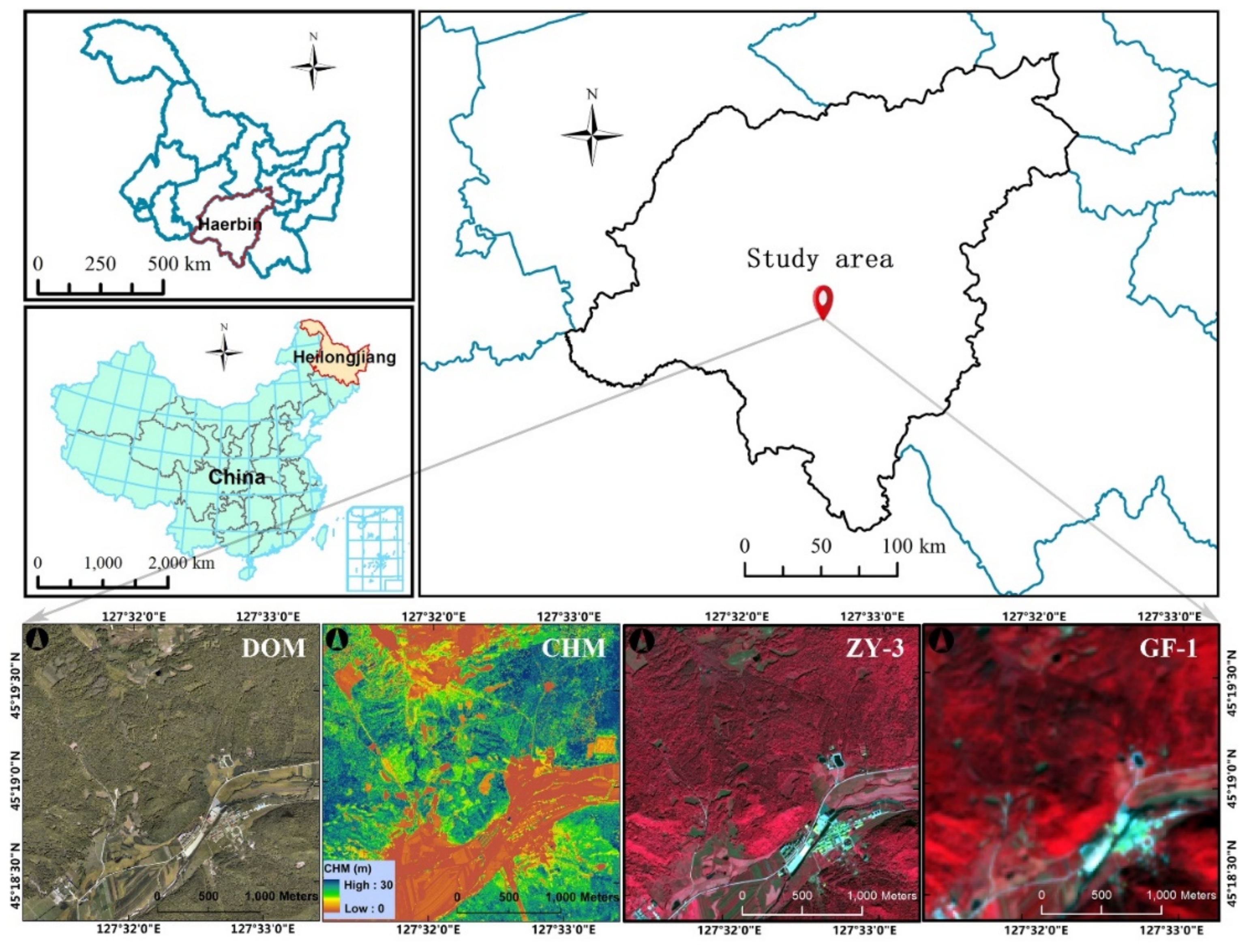
The study area is the Maoershan Experimental Forest Farm (45°15′–45°29′ N, 127°23′–127°43′ E) in Shangzhi City, Heilongjiang Province, China, with a total area of approximately 26,000 ha. From the perspective of flora, this area belongs to the Changbai Mountain flora of China. The zonal species in this area is a typical Korean pine broad-leaved mixed forest composed mainly of Korean pine (Pinus koraiensis). The original forest of the area began to suffer a lot of serious damage when they built the Middle East Railway in 1906, resulting in barren hills, shrubs, swamps and remnants of different degrees of damage. After 1949, under the rational management, all kinds of secondary forest communities have been naturally restored and developed, forming a typical natural secondary forest in Northeastern China. The secondary forests are diverse and representative, and the community types include hard broad-leaved forests, soft broad-leaved forests, coniferous forests and coniferous and broad-leaved mixed forests. The experimental area is a rectangular area with a side length of 2880 m in the Maoershan Experimental Forest, with a total area of approximately 829 ha (Figure 1). The main reason for selecting this area as the experimental area is that the landscape in the area has a high diversity. The landscape includes forest, grassland and farmland, and the spatial distribution characteristics of the vegetation are obvious. In addition, there are roads, rivers, buildings, bare land and other different types of object.
2.2. Remote Sensing Data
This study used GF-1, ZY-3 multispectral and full-color remote sensing images, combined with airborne LiDAR data and aerial orthophotos to provide the different special-resolution required for research and analysis and verification (Table 1). LiDAR data acquisition uses the LiCHy airborne observing system. The system integrates LiDAR ranging, aerial imagery, hyperspectral data acquisition, global positioning system (GPS) and inertial navigation system (INS). The LiDAR uses the Riegl LMS-Q680i (Riegl, Horn, Austria) full-waveform LiDAR scanner and the CCD camera uses the Digi CAM-60 (IGI, Kreuztal, Germany) digital aerial camera [42]. The flight platform adopted the domestically-operated-10 aircraft, and the collection time was from September 14 to 15, 2016. The weather was clear and cloudless during data collection. The average density of point cloud data was 3.7 point/m2 and the acquired aerial image was obtained simultaneously with the resolution of 0.2 m, and the data was used as a reference sample and a reference and basis for classification accuracy verification.
Using the adaptive Triangular Irregular Networks (TIN) model filtering of TerraScan software (Terrasolid, Heisinki, Finland), the original LiDAR point cloud data was divided into ground point cloud and non-ground point cloud. The inverse distance weight method was used to interpolate the ground point and the first echo point cloud to generate the 0.5 m and 2.1 m digital elevation model (DEM), digital surface model (DSM) and fractional canopy cover (FCC). Compared with the differential GPS measured elevation, the acquired LiDAR data had a vertical accuracy better than 0.3 m and a horizontal accuracy better than 0.5 m. The DSM and DEM were subtracted to obtain a canopy height model (CHM) and normalized so that the pixel values were between 0 and 1. Although the LiDAR point cloud was modified in the generation of DSM and DEM, the generated CHM still had some errors, especially it contains many dramatic height mutations, especially in the middle of the canopy. Jakubowski et al. [43] proposed a process that combines the idea of morphological closure and mathematical mask replacement to effectively improve the error of the original CHM. This study adopted this method, and a new set of parameters was used in combination with the CHM data used. After correction, CHM removed more than 95% of the high-mutation troughs. The data types of all raster maps are 32-bit floating point type, both using the WGS-84 (World Geodetic System-1984) geographic coordinate system and the universal transverse axis Mercator (UTM) projected coordinate system, consistent with the remote sensing image coordinate system.
The preprocessing of ZY-3 and GF-1 multispectral images mainly includes radiometric calibration, atmospheric correction, orthorectification, image registration, image fusion and terrain correction. The study was based on the radiometric calibration coefficients of ZY-3 and GF-1 satellites released by the China Resources Satellite Application Center (http://www.cresda.com/CN/). Atmospheric correction removes the error caused by the scattering, absorption and reflection of the atmosphere from the apparent reflectivity and obtains the surface reflectivity, which is the reflectivity of the real object. In this study, the dark-objects algorithm was used for atmospheric correction [44]. Using the aerial orthophoto image as a reference, the ortho-correction of ZY-3 and GF-1 was performed using LiDAR-extracted 2.1 m DEM. In this study, ZY-3 multispectral data and panchromatic images were fused to a 2.1 m resolution data using the GS fusion method [45]. Due to the complex terrain in the study area, the DEM extracted by LiDAR was used for terrain correction using the C-correction method [46,47,48].
2.3. Methods
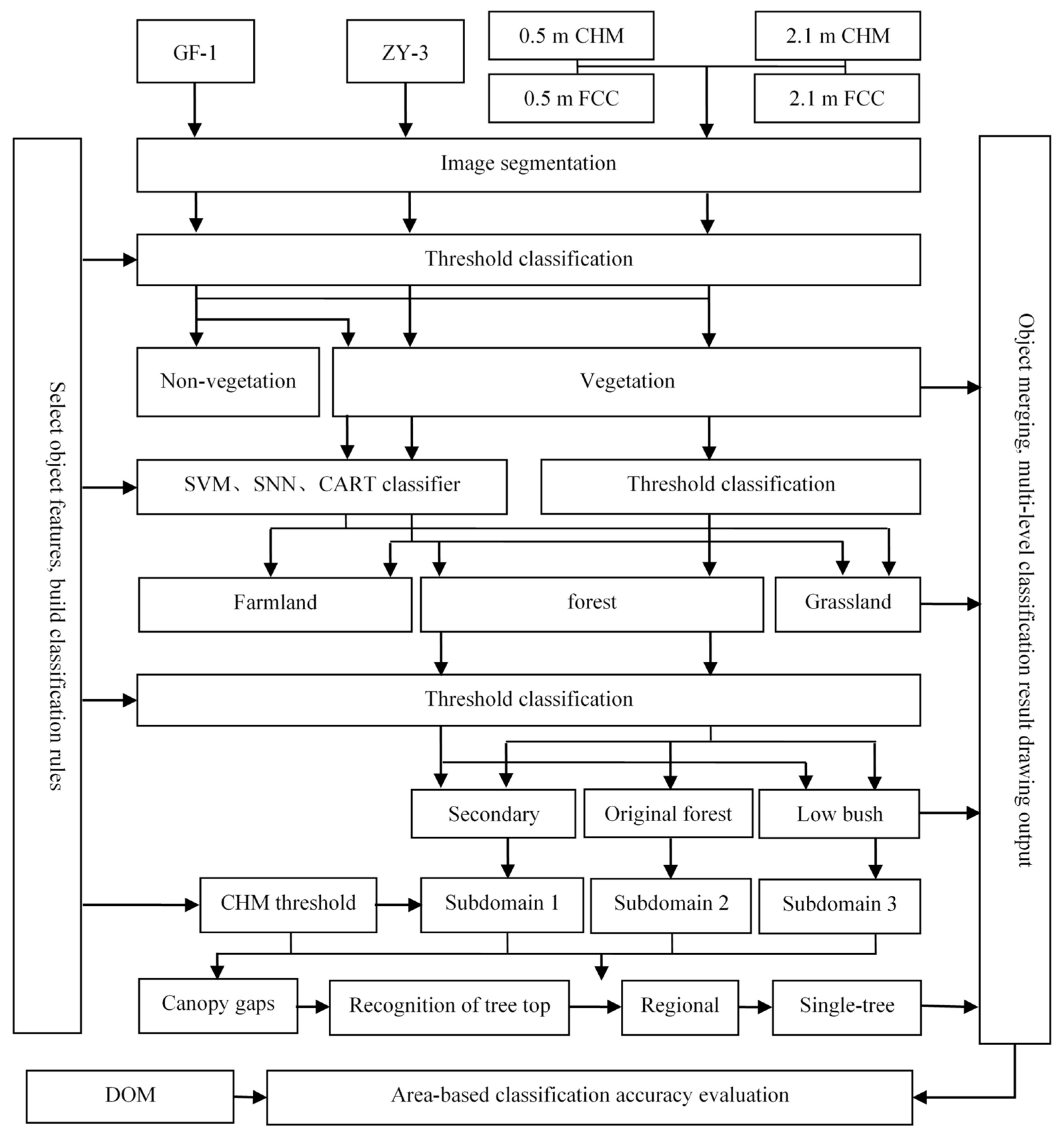
Multi-scale vegetation type classification must first establish a multi-level classification system. In this study, vegetation information was classified into four levels: the first layer was the vegetation and non-vegetation layer (L1); the second layer was divided into farmland and grassland and forest, called the vegetation type layer (L2); the third layer was divided into secondary forest and original forest, called the forest type (L3) and the fourth layer was canopy and the canopy gaps (L4). To complete multi-scale vegetation type extraction, the GEOBIA technique was used in this study. The main reasons are: (1) image objects can be created on multiple specific hierarchical spatial scales (for example, forest stands are composed of multiple canopy layers); (2) image objects can obtain many attributes (statistics, geometry and structure of objects); (3) GEOBIA technique can better imitate people’s perception of real-world objects; (4) image classification reduces the phenomenon of salt-and-pepper effect and (5) output (classification object) can be directly used for spatial analysis of geographic information systems. This study used eCognition Developer 8.7 (Trimble Germany GmbH, Munich, Germany) to develop a classification rule set and perform an object-oriented processing flow. The technical route is shown in Figure 2.
2.4. Vegetation and Non-Vegetation Separation
The first stratification of multi-scale vegetation type classification separated the vegetation objects from the non-vegetation objects (water, bare soil and artificial surface). In this study, the forest discrimination index (FDI, FDI = NIR − (Red + Green)) was combined with the normalized difference vegetation index (NDVI) to distinguish vegetation from non-vegetation features for GF-1 and ZY-3 [40,49]. Although the spectral bands of GF-1 and ZY-3 images are the same, there are differences in spectral reflectance of ground objects between different images, and different classification thresholds are used for the two. 2.1 m and 0.5 m CHM and 2.1 m and 0.5 m FCC were used to extract vegetation and non-vegetation for LiDAR data. It is found that the value of FCC representing vegetation coverage can effectively distinguish vegetation from non-vegetation. After multiple experiments, the threshold value was determined to complete the extraction of vegetation objects, and the vegetation and non-vegetation distribution map based on LiDAR data was obtained (Table 2-L1).
2.5. Vegetation Type Distinction
This study attempted to extract vegetation types from GY-1 and ZY-3 remote sensing images using the SVM classifier, standard nearest neighbor (SNN) classifier and CART classifier. Additionally, the effects of spatial resolution and classification methods on the results were compared. The vegetation type distribution map based on GF-1 and ZY-3 was obtained by manually selecting the same set of samples for use with three types of classifiers in conjunction with aerial orthophotos. In order to explore the relationship between LiDAR data and image data and different resolution data and classification results, a classification rule was constructed for CHM and FCC of two resolutions to divide vegetation objects into forest, grassland and farmland (Table 2-L2). After many experiments, it was found that the use of vegetation height features can accurately identify the forest, and the spectral difference segmentation can be applied to the original segmentation results to separate and extract the discrete forest trees (single or grouped trees). However, the use of CHM and FCC only in the L2 layer does not effectively distinguish grassland from farmland. The reasons are as follows: first, the height of crops planted is not consistent; second, it is affected by the growth of crops, and its coverage is confused with grassland formation. In this study, farmland was extracted first, and the remaining layer of the object was set to grassland. Finally, farmland and forest less than a certain area were classified as grassland as the misclassification object, and the vegetation community type distribution map based on LiDAR data was obtained.
2.6. Forest Type Distinction
Due to the low spatial resolution of the image and the high density of forest vegetation, GF-1 remote sensing images cannot distinguish specific forest type. Therefore, only the ZY-3 and LiDAR data were processed in this layer (L3; Table 2-L3). The main basis for distinguishing forest is the change in stand height and density caused by natural or artificial disturbances. The gaps in the forest are the key factor determining the density of the stand, where the density structure of the stand can be measured by the standard deviation of the image objects. For LiDAR data, shrub can be identified directly by the average height of the canopy. Since original forest are not disturbed, the average canopy height is high and the canopy is closed, the mean and standard deviation of CHM are selected as features to classify original forest and secondary forest. For the ZY-3 image, in order to obtain the spectral information of the image to the greatest extent, the first principal component (PCA1) was used as the basis to rescale the multiresolution segmentation (MRS) of the best forest classification result of the L2 layer. Considering that the vegetation had the highest reflectance in the near-infrared (NIR) band, the NIR mean and standard deviation were selected to classify the forest.
2.7. Canopy and Canopy Gap Extraction
In this study, the “valley tracking” and “regional growth” methods were used to extract canopy and canopy gaps [50]. The main theoretical basis for extracting the canopy and canopy gaps is that the regions refer to “valleys” in the figure have relatively low spectral reflectance or height values, so they represent the interstitial spaces; while the “top” has a locally higher spectral reflectance or height values, so they represent the canopy of a single-tree. This method of delineating the canopy and canopy gap has two prerequisites: one is that the pixel size of the image is much smaller than the average size of the canopy, and the other is that the pixel value of the canopy is higher than the pixel value around the canopy. The resolution of ZY-3 image does not meet this premise. Therefore, this study only extracted a single-tree canopy from 0.5 m CHM.
In order to reduce the processing time and study the different results of the single forest canopy for different forest types, this study selected a small representative area from each of the three forest areas delineated by the L3 layer. First, the chessboard segmentation was performed for each experimental area to obtain height information for a single cell and then perform a canopy sketch (Table 2-L4). The generation of the single-tree canopy was completed in three steps. First, the gap area around the canopy was determined by the threshold as the boundary of the area growth. Then look for a certain range of height maxima (top of the tree) as a seed point and filter out the non-conformity (below the canopy threshold or less than or equal to 1 m from the gap area). The seed point was then fused to the surrounding candidate points based on the ratio of the seed point height value to the height value of the neighboring points. A loop iterative process was performed when the generated canopy region satisfied an aspect ratio of less than 2.3 and the area was less than a certain threshold until the condition was not met or the growth boundary was reached. After the completion of this step, a distribution map of single-tree canopy and canopy gaps in three forest stands based on CHM was generated.
2.8. Classification Accuracy Evaluation
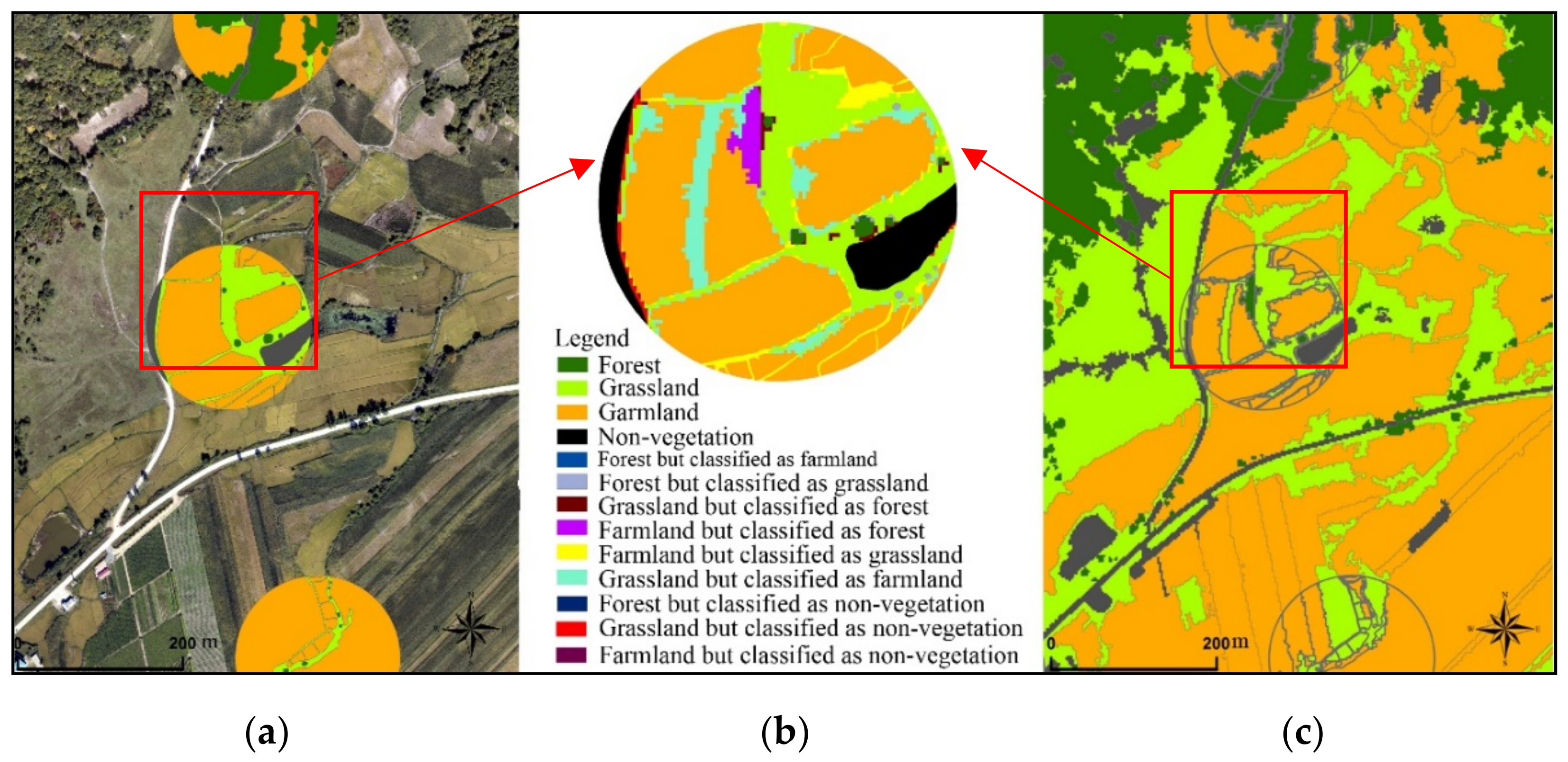
GEOBIA’s accuracy assessment requires an assessment of the geometric accuracy (shape, symmetry and position) of the created image object. Zhan et al. [51] and Whiteside et al. [52] designed a framework for evaluating the geometric properties of image objects based on the error matrix. According to this method, the accuracy evaluation scheme based on the object area was adopted. The classification result maps of the 1 L to 4 L layers were compared with the local reference polygon vector diagrams, and the area difference estimation of each category was performed separately. Given the different scales of each layer of image objects, different ranges of reference polygon data were required on different layers. Referring to the Whiteside’s method, for the L1 and L2 layers, 30 points were randomly selected in the reference map as a circular buffer with a radius of 100 m as the verification area, and each type of vector polygon was used as a sample to superimpose and intersect the classification results (Figure 3). Similarly, for the L3 and L4 layers, 15 and 10 points were randomly selected in the verification range as circular buffers with a radius of 50 m and 5 m, respectively. Through the comparison of the total area of the verification area, the corresponding producer accuracy (PA, Equation (1)), user precision (UA, Equation (2)), total accuracy of single class (TA, Equation (3)) and overall accuracy (OA, Equation (4)) of each class were calculated.
For optical remote sensing images (GF-1, ZY-3), the spectral reflectance of images was the main basis for distinguishing between vegetation and non-vegetation. Considering that the ZY-3 remote sensing image acquisition time is one year earlier than the other original and verified data, many bare lands that appeared as non-vegetation in ZY-3 images were vegetated after a year with crops. In order to avoid systematic misclassification of the verification data in the ZY-3 image accuracy verification, the classification results were processed in this study, and the farmland with changed farming conditions was excluded from the verification area, thus avoiding the interference of time inconsistency on the verification results.
Among them, S represents the area of a polygonal object, Ci represents the classified object of class i, Ri represents the reference object of class i, ∩ represents the intersection of the two and ∪ represents the union of the two.
3. Results
3.1. Vegetation and Non-Vegetation Extraction Results
Using the FDI and NDVI in the L1 layer, the vegetation and non-vegetation were successfully separated, and the OA was 88% (GF-1) and 94% (ZY-3) respectively (Table 3-L1). The vegetation in the ZY-3 classification map shows a more precise boundary than the GF-1 classification map, and the area misclassified as non-vegetation was significantly reduced (Figure 4-L1 layer). With the increase of spatial resolution, the TA of ZY-3 images to non-vegetation single class was 15% higher than that of GF-1 images, and the TA of vegetation was 10% higher. For LiDAR data, the main basis for classification in this layer was FCC. Using FCC features, the vegetation coverage area could be extracted very completely, with an OA of 97% (2.1 m LiDAR) and 98% (0.5 m LiDAR) respectively (Table 3-L1). The improvement of image resolution had improved the recognition accuracy of non-vegetation by 7%, while the recognition of vegetation had not changed significantly. The OA of the 2.1 m LiDAR was 3% higher than the ZY-3 image with the same resolution, while the total classification accuracy of the ZY-3 image was 16% higher than the GF-1 image.
3.2. Vegetation Type Classification Results
For GF-1 images, SVM, SNN and CART classifiers had the best TA (84%) for forest, followed by farmland (35–42%) and the worst was grassland (9–22%). It can be clearly seen from the layer of Figure 4-L2 that a large number of grasslands were divided into farmland, and some farmland was misclassified into grassland. Mixed pixels formed by low image resolution had a great influence on spectral recognition and restricted the extraction of vegetation type seriously. At the same time, it was found that the SNN classifier had the best classification effect on grassland and farmland, and the TA was 13% and 5% higher than that of the SVM classifier, and 12% and 7% higher than the CART classifier. This also shows that the SNN classifier had the strongest ability to separate similar targets, and was most suitable for distinguishing features with small spectral differences. The SVM and CART classifiers had the same recognition accuracy for the three plant types, and the three classifiers had a small difference in the OA of the layer (66–69%). Overall, the SNN classifier had the best classification effect on GF-1. For the ZY-3 image, to eliminate the interference, the farmland that also changed was excluded from the accuracy verification. The three classifiers also had the best OA (80–83%) for the forest, and the discrimination effect on the grassland and the farmland was still not ideal. Among the three classifiers, SNN had the best recognition effect on forest (OA = 83%), SVM had the best recognition effect on grassland (TA = 31%) and CART had the best recognition effect on farmland (TA = 45%). The overall classification accuracy of the three classifiers in this layer was roughly the same, and the SNN classifier was generally better.
For two resolutions of LiDAR data, 2.1 m LiDAR could extract many small vegetation areas, while 0.5 m LiDAR was more refined, and even could extract weeds in the field. Both resolutions of LiDAR data achieved high OA of 89% (2.1 m) and 93% (0.5 m), respectively. The two LiDAR data were similar to the optical remote sensing images, which had the best recognition effect on forest (94% and 96%), followed by farmland (70% and 83%) and the worst on grassland (60% and 72%) (Table 3-L2). The comprehensive comparison of optical remote sensing images and LiDAR data classification results shows that with the improvement of remote sensing image resolution, the OA of this layer was only increased by 4–6%. With the improvement of LiDAR data resolution, the OA was only improved by 4%; however, the use of LiDAR data compared to the use of remote sensing images of the same resolution, resulting in an OA increased by 16–17%.
3.3. Classification of Forest Type
The spectral reflectance of the near-infrared band of ZY-3 was used to characterize the structural condition classification results of the stand (Figure 4-L3). The extraction effect of the forest type was poor, and most of the forest was misclassified, the OA was only 25%. The TA of the original forest stand and secondary forest stand was even lower than 15%, and the classification accuracy of shrub forest was slightly higher. The results show that on the forest type scale, the spectral information of remote sensing images was unable to obtain meaningful extraction results, and it is necessary to use physical information that can visually reflect the structure of the forest. The 2.1 m LiDAR data and 0.5 m LiDAR data were more detailed in the classification of different forest types, and the secondary forest and shrub forest were successfully extracted. The OA of the two types of LiDAR data for forest type was 68% (2.1 m) and 80% (0.5 m) respectively. Among the three forest types, the TA of low shrub stands was the highest (59% and 75%), followed by secondary forest (55% and 69%) and original forest (46% and 60%). This also reflects the feature of canopy height that can extract shrubs relatively accurately. By comparing LiDAR data with ZY-3 image classification results, it was found that the classification result of forest type using 2.1 m LiDAR was improved by 43% compared with the same resolution ZY-3 image.
3.4. Canopy and Canopy Gaps Distribution
In this study, the canopy and canopy gaps were extracted using 0.5 m CHM. To compare the effects of the three forest types on the extraction results, three representative forest plots were selected for experiment (Figure 4-L4). The OA of 66% (original forest), 70% (secondary forest) and 71% (shrub forest) was obtained for the three forest types. The accuracy verification results were analyzed. It was found that although the total precision of the canopy and canopy gaps extraction of the original forest was the lowest, it had the highest OA of the single canopy (83%), and the low comprehensive extraction accuracy was caused by only 13% of the TA of canopy gaps. The OA of canopy gaps extraction in original forest, secondary forest and shrub was relatively close, but the TA of canopy extraction was 9% higher than that of secondary forest. The TA of canopy gaps extraction in this layer was 55% higher and the OA was 4% higher than that in the original forest division (Table 3-L4).
3.5. Classification Accuracy Comparison
On the L1 layer, whether it was an optical remote sensing image or LiDAR data, with the increase of spatial resolution, both OA and TA increased synchronously and remained at a high level. However, the LiDAR data still maintained this mode on the L2 layer, but the optical remote sensing image shows that the TA did not rise and fall for the forest and farmland, which is related to the fact that the classification sample changes and the ZY-3 verification area were partially ignored. In the LiDAR data on this layer, the OA remained at a high level close to 90%, while the OA of the optical remote sensing image data was reduced to 65–75%. At the L3 level, the OA and TA of the LiDAR data continued to rise with increasing resolution; but remained at a medium to high level (68–80%). On the L4 layer, except for the original canopy gaps, both OA and TA were between 60% and 80%. The results indicate that the rule set established for these two layers could not be very properly classified on the forest type and the single-tree. Throughout the whole, the results of the area-based accuracy assessment method not only evaluated the quantitative relationship of the classification target, but also verified the geometric accuracy of the target object boundary relative to the verification data.
4. Discussion
4.1. Attributive Analysis of Classification Results
The optical classification images (GF-1 and ZY-3) were used to obtain better classification results on the L1 layer (vegetation non-vegetation layer), indicating that FDI could better identify all types of vegetation. NDVI has some saturation problems for vegetation identification and FDI is a good complement. LiDAR obtained better classification accuracy than optical data, indicating that the physical characteristics of vegetation (vegetation coverage) could provide more accurate information than spectral features, and was more effective for vegetation identification. In addition to the data source, image spatial resolution was the main factor that constrains the classification accuracy of this layer.
In the L2 layer (vegetation type layer), no matter whether using optical remote sensing image or LiDAR data, the farmland and grassland classification had not achieved satisfactory results. The main reason is that the spectral characteristics of grassland are very similar to farmland, and the degree of vegetation coverage between grassland and farmland. There is a certain degree of intersection with the height, and the use of a certain series of thresholds will have limitations. The classification accuracy of using the same data source (GF-1 vs. ZY-3 and 2.1 m LiDAR vs. 0.5 m LiDAR) was improved to some degree (4–6%) with the increase of spatial resolution for the L2 layer. However, the classification accuracy of using the same resolution but different data sources (2.1 m ZY-3 and 2.1 m LiDAR data) could be improved by two digits (16–17%). The results show that on the spatial scale of vegetation type, the data resolution is not the main factor affecting the classification accuracy, and the vegetation information that the data can provide becomes the dominant factor determining the classification effect. Compared with the single spectral information provided by optical remote sensing images, active LiDAR remote sensing can provide important information about the physical characteristics of vegetation in the target area, such as vegetation cover density and vegetation height, which are powerful tools to help identify forest type and effectively improve the classification accuracy.
It is difficult to classify the forest type corresponding to a single forest in the L3 layer (forest type), especially in the case of simply using spectral information. In theory, the texture information of remote sensing images can be used as the basis for discrimination. However, this study was not applicable to ZY-3 images because there were a lot of shadows in the 2.1 m resolution image, which led to difficulty using image texture features to extract information from the L3 layer. The classification result of forest type using 2.1 m LiDAR was greatly improved (43%) than that of ZY-3 image. This shows that only the physical features that could characterize the stand structure could be used to identify specific forest areas on this layer scale, and the 2.1 m level resolution remote sensing image was not enough to provide sufficient spectral information to accomplish this task. More spectral images of CHM data provide more detailed and accurate vertical (horizontal) structural information of the stand. Therefore, using CHM on the three forest type (L3 layer) could obtain meaningful results while the impact of using the same resolution ZY-3 was not the case.
In the extraction of canopy and canopy gaps (L4 layer), the TA of the canopy gaps in the secondary forest area was more than 50% higher than that of the original forest, mainly because the secondary forest had higher forest structure. Since the height of the shrub area was low and similar, the shrub stand experimental area had the lowest vegetation structure diversity, which is difficult to accurately express the structural changes of the shrub stand relative to other stand types, so in the ZY-3 image PCA1 it is impossible to distinguish between shrubs and canopy gaps; however, in the CHM, the shrubs and shrubs can be better identified. The shrubs are relatively independent in space and there is little overlap between the canopies, so the actual layer L4. In the extraction results, the shrub division obtained the highest total classification accuracy.
4.2. Spatial Resolution and the Impact of Data Sources on Classification
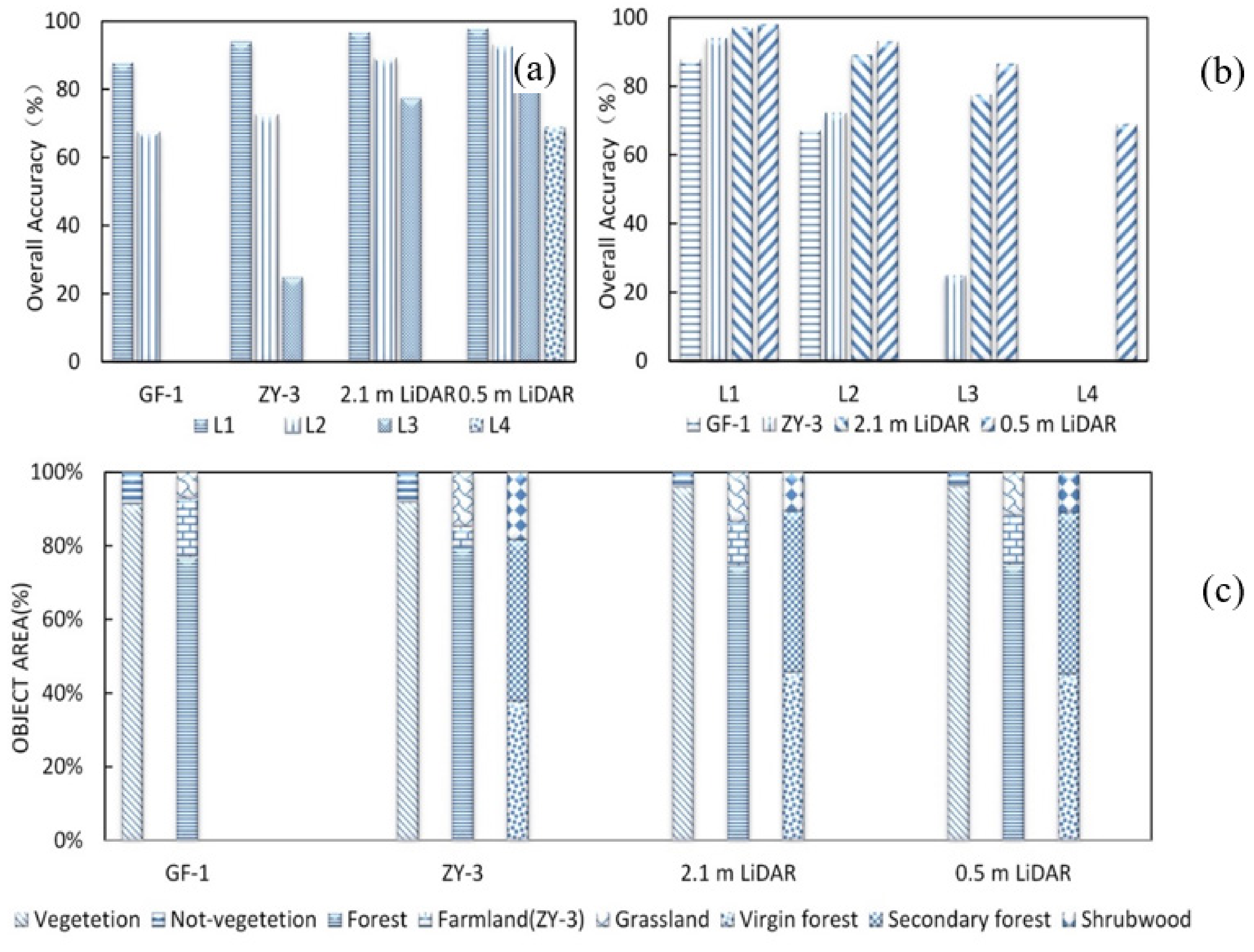
The resolution of remote sensing images and LiDAR data had an obvious impact on the classification results of this study. Classification results indicate that low-resolution data had some limitations in the ability to express vegetation features compared to high-resolution data. GF-1 imagery (16 m) and ZY-3 imagery (2.1 m) were able to distinguish vegetation types, while 0.5 m CHM was able to extract more detailed vegetation features on a single-tree. The low spatial resolution of the resulting mixed pixels results in poor spectral heterogeneity [53], which not only directly reduces the sensitivity of identifying complex objects but also the ability to extract small objects [54]. On the other hand, the information content that remote sensing images and LiDAR data can provide is also very different, especially in the detail level of vegetation characteristics. There were also differences in the proportion of different categories of different data on the different classes in the parent class (Figure 5c). It can be seen that the area ratio of the various types of area formed by LiDAR data and the area ratio of remote sensing image classification had changed significantly. However, the use of remote sensing data or LiDAR data of different resolutions yielded roughly the same area ratio. This result not only shows that the type of data source had a great influence on the classification accuracy, but also played an important role in the classification quantity characteristics.
The total classification accuracy of the ZY-3 images on the L2 layer using the three classifier results was averaged and used as the average total classification accuracy on the layer to participate in the comparison chart. As the resolution of the data increased, the overall classification accuracy increased and the use of LiDAR data resulted in higher overall classification accuracy than using remote sensing images (Figure 5a). On the other hand, with the deepening of the classification hierarchy (the scale is more refined), the overall classification accuracy of all data was decreasing in turn (Figure 5b). The explanation for this phenomenon was as follows: First, the target object of a smaller scale needs to be formulated with more complicated classification rules, and a single rule set may not be able to accurately achieve the target. Secondly, small-scale targets will produce relatively large internal differences in the class, which will reduce the separation of their spectral or physical properties and cause a decrease in classification accuracy [55]. Last but not least, the general classification accuracy will decrease as the number of categories is increased [56], because a larger proportion of overlapping parts will be at the boundary of the actual object after the target object category increases. This phenomenon is called the “boundary effect” and thus affects the overall classification accuracy.
4.3. Classification Rules and Their Impact on Classification
The development of an efficient classification rule set requires a clear understanding of the spatial, physical and hierarchical characteristics of vegetation target objects [37]. In this study, the rule sets of spectral, geometric, class-related and process-related attributes of image objects were used in each level to construct the rule set, which can maximize the information implied by the target object and help improve the classification accuracy. However, the rule set is still not independent of the data set and processing area. Due to the spectral reflectance and the type of information between the data, different data needs to apply different algorithms, parameters or thresholds for similar target objects. Additionally, because of different environmental conditions, local vegetation structure variations and spectral physical information differences at specific locations, algorithms, parameters or thresholds need to be adjusted for target objects with similar locations. The accuracy of vegetation type extraction in this study was determined by the combination of data type, data resolution, scale of classification target object, location of parent category object and number of land cover categories to be classified [40].
5. Conclusions
Spatial distribution information of multiscale forest vegetation is of great significance for the management and protection of forest ecosystems on related scales. This study compared the efficacy of using GF-1 and ZY-3 remote sensing images and airborne LiDAR data with two resolutions to extract multiscale information on the vegetation characteristics of natural secondary forest in Northeastern China. The results showed that high spatial resolution LiDAR data could obtain more detailed vegetation information. Moreover, the results also showed that the physical information of vegetation height and density provided by the LiDAR data could produce category extraction more efficiently in comparison with the spectral information provided by optical remote sensing images. It was also found that on the large spatial scale (vegetation and non-vegetation layer), the spatial resolution of the dataset played a leading role in the classification results, while on the smaller spatial scale, the type of data used was the main factor affecting the type extraction. GF-1 and ZY-3 images could only be used to obtain meaningful results in terms of distinguishing vegetation type. Conversely, use of the LiDAR data could obtain more detailed vegetation features, including delineation of forest type and extraction of canopies and canopy gaps. The results obtained in this study were limited by the selected image data and the location of the study area. Further research should include the use of submeter high-resolution remote sensing images to participate in geographic object-oriented analysis. Furthermore, the workflow method proposed in this study should be applied to a non-forest-based ecosystem environment to test the portability of the four hierarchical models in terms of spatial position. Finally, this research was partly affected by inconsistency in the time of image data acquisition. Further research should be undertaken to determine the relationship between temporal change and the type extraction capability of landscape structure units.
Author Contributions
Conceptualization, Y.D. and X.M.; methodology, Y.D. and X.M.; software, Y.Y.; validation, L.Z.; writing—original draft preparation, Y.D.; writing—review and editing, Y.D. and X.M.; funding acquisition, X.M. All authors have read and agreed to the published version of the manuscript.
Funding
This work is jointly supported by the State Key Laboratory of Subtropical Silviculture (KF202003) and the Fundamental Research Funds for the Central Universities (2572018BA02).
Acknowledgments
We thank James Buxton MSc from Liwen Bianji, Edanz Group China (www.liwenbianji.cn./ac), for editing the English text of this manuscript.
Conflicts of Interest
The authors declare no conflict of interest.
References
- Lehnert, L.W.; Meyer, H.; Wang, Y.; Miehe, G.; Thies, B.; Reudenbach, C.; Bendix, J. Retrieval of grassland plant coverage on the Tibetan Plateau based on a multi-scale, multi-sensor and multi-method approach. Remote Sens. Environ. 2015, 164, 197–207. [Google Scholar] [CrossRef]
- Van Beijma, S.; Comber, A.; Lamb, A. Random forest classification of salt marsh vegetation habitats using quad-polarimetric airborne SAR, elevation and optical RS data. Remote Sens. Environ. 2014, 149, 118–129. [Google Scholar] [CrossRef]
- Liu, T.; Yang, X. Mapping vegetation in an urban area with stratified classification and multiple endmember spectral mixture analysis. Remote Sens. Environ. 2013, 133, 251–264. [Google Scholar] [CrossRef]
- Immitzer, M.; Atzberger, C.; Koukal, T. Tree Species Classification with Random Forest Using Very High Spatial Resolution 8-Band WorldView-2 Satellite Data. Remote Sens. 2012, 4, 2661–2693. [Google Scholar] [CrossRef] [Green Version]
- Laurin, G.V.; Puletti, N.; Hawthorne, W.; Liesenberg, V.; Corona, P.; Papale, D.; Chen, Q.; Valentini, R. Discrimination of tropical forest types, dominant species, and mapping of functional guilds by hyperspectral and simulated multispectral Sentinel-2 data. Remote Sens. Environ. 2016, 176, 163–176. [Google Scholar] [CrossRef] [Green Version]
- Naidoo, L.; Cho, M.; Mathieu, R.; Asner, G.P. Classification of savanna tree species, in the Greater Kruger National Park region, by integrating hyperspectral and LiDAR data in a Random Forest data mining environment. ISPRS J. Photogramm. Remote Sens. 2012, 69, 167–179. [Google Scholar] [CrossRef]
- Treitz, P. High Spatial Resolution Remote Sensing Data for Forest Ecosystem Classification An Examination of Spatial Scale. Remote Sens. Environ. 2000, 72, 268–289. [Google Scholar] [CrossRef]
- Krause, G.; Bock, M.; Weiers, S.; Braun, G. Mapping Land-Cover and Mangrove Structures with Remote Sensing Techniques: A Contribution to a Synoptic GIS in Support of Coastal Management in North Brazil. Environ. Manag. 2004, 34, 429–440. [Google Scholar] [CrossRef]
- Zhu, Z.; Woodcock, C.E.; Olofsson, P. Continuous monitoring of forest disturbance using all available Landsat imagery. Remote Sens. Environ. 2012, 122, 75–91. [Google Scholar] [CrossRef]
- Coulter, L.L.; Stow, D.A.; Tsai, Y.-H.; Ibanez, N.; Shih, H.-C.; Kerr, A.; Benza, M.; Weeks, J.R.; Mensah, F. Classification and assessment of land cover and land use change in southern Ghana using dense stacks of Landsat 7 ETM+ imagery. Remote Sens. Environ. 2016, 184, 396–409. [Google Scholar] [CrossRef]
- Liu, X.; Bo, Y.; Zhang, J.; He, Y.Q. Classification of C 3 and C4 vegetation types using MODIS and ETM+ blended high spatio-temporal resolution data. Remote Sens. 2015, 7, 15244–15268. [Google Scholar] [CrossRef] [Green Version]
- Van Coillie, F.; Verbeke, L.; Dewulf, R. Feature selection by genetic algorithms in object-based classification of IKONOS imagery for forest mapping in Flanders, Belgium. Remote Sens. Environ. 2007, 110, 476–487. [Google Scholar] [CrossRef]
- Pu, R.; Landry, S. A comparative analysis of high spatial resolution IKONOS and WorldView-2 imagery for mapping urban tree species. Remote Sens. Environ. 2012, 124, 516–533. [Google Scholar] [CrossRef]
- Feng, Y.; Lu, D.; Moran, E.; Dutra, L.V.; Calvi, M.F.; De Oliveira, M.A.F. Examining Spatial Distribution and Dynamic Change of Urban Land Covers in the Brazilian Amazon Using Multitemporal Multisensor High Spatial Resolution Satellite Imagery. Remote Sens. 2017, 9, 381. [Google Scholar] [CrossRef] [Green Version]
- Masek, J.G.; Huang, C.; Wolfe, R.; Cohen, W.; Hall, F.; Kutler, J.; Nelson, P. North American forest disturbance mapped from a decadal Landsat record. Remote Sens. Environ. 2008, 112, 2914–2926. [Google Scholar] [CrossRef]
- Li, J.; Mao, X. Comparison of Canopy Closure Estimation of Plantations Using Parametric, Semi-Parametric, and Non-Parametric Models Based on GF-1 Remote Sensing Images. Forests 2020, 11, 597. [Google Scholar] [CrossRef]
- Li, N.; Lu, D.; Wu, M.; Zhang, Y.; Lu, L. Coastal wetland classification with multiseasonal high-spatial resolution satellite imagery. Int. J. Remote Sens. 2018, 39, 8963–8983. [Google Scholar] [CrossRef]
- Kim, M.; Warner, T.A.; Madden, M.; Atkinson, D.S. Multi-scale GEOBIA with very high spatial resolution digital aerial imagery: Scale, texture and image objects. Int. J. Remote Sens. 2011, 32, 2825–2850. [Google Scholar] [CrossRef]
- Powers, R.P.; Hay, G.J.; Chen, G. How wetland type and area differ through scale: A GEOBIA case study in Alberta’s Boreal Plains. Remote Sens. Environ. 2012, 117, 135–145. [Google Scholar] [CrossRef]
- Sasaki, T.; Imanishi, J.; Ioki, K.; Morimoto, Y.; Kitada, K. Object-based classification of land cover and tree species by integrating airborne LiDAR and high spatial resolution imagery data. Landsc. Ecol. Eng. 2011, 8, 157–171. [Google Scholar] [CrossRef]
- Zhou, W.; Troy, A. An object-oriented approach for analysing and characterizing urban landscape at the parcel level. Int. J. Remote Sens. 2008, 29, 3119–3135. [Google Scholar] [CrossRef]
- Burnett, C.; Blaschke, T. A multi-scale segmentation/object relationship modelling methodology for landscape analysis. Ecol. Model. 2003, 168, 233–249. [Google Scholar] [CrossRef]
- Ke, Y.; Quackenbush, L.J.; Im, J. Synergistic use of QuickBird multispectral imagery and LIDAR data for object-based forest species classification. Remote Sens. Environ. 2010, 114, 1141–1154. [Google Scholar] [CrossRef]
- Demarchi, L.; Bizzi, S.; Piegay, H. Hierarchical Object-Based Mapping of Riverscape Units and in-Stream Mesohabitats Using LiDAR and VHR Imagery. Remote Sens. 2016, 8, 97. [Google Scholar] [CrossRef] [Green Version]
- Xuegang, M.; Liang, Z.; Fan, W. Object-Oriented Automatic Identification of Forest Gaps Using Digital Orthophoto Maps and LiDAR Data. Can. J. Remote Sens. 2020, 46, 177–192. [Google Scholar] [CrossRef]
- Mao, X.; Hou, J. Object-based forest gaps classification using airborne LiDAR data. J. For. Res. 2019, 30, 617. [Google Scholar] [CrossRef]
- Ma, L.; Li, M.; Ma, X.; Cheng, L.; Du, P.; Liu, Y. A review of supervised object-based land-cover image classification. ISPRS J. Photogramm. Remote Sens. 2017, 130, 277–293. [Google Scholar] [CrossRef]
- Drăguţ, L.; Csillik, O.; Eisank, C.; Tiede, D. Automated parameterisation for multi-scale image segmentation on multiple layers. ISPRS J. Photogramm. Remote Sens. 2014, 88, 119–127. [Google Scholar] [CrossRef] [Green Version]
- Mallinis, G.; Koutsias, N.; Tsakiri, M.; Karteris, M. Object-based classification using Quickbird imagery for delineating forest vegetation polygons in a Mediterranean test site. ISPRS J. Photogramm. Remote Sens. 2008, 63, 237–250. [Google Scholar] [CrossRef]
- Qi, Z.; Yeh, A.G.-O.; Li, X.; Lin, Z. A novel algorithm for land use and land cover classification using RADARSAT-2 polarimetric SAR data. Remote Sens. Environ. 2012, 118, 21–39. [Google Scholar] [CrossRef]
- Dalponte, M.; Ørka, H.O.; Ene, L.; Gobakken, T.; Næsset, E. Tree crown delineation and tree species classification in boreal forests using hyperspectral and ALS data. Remote Sens. Environ. 2014, 140, 306–317. [Google Scholar] [CrossRef]
- Xie, Z.; Chen, Y.; Lu, D.; Li, G.; Chen, E. Classification of Land Cover, Forest, and Tree Species Classes with ZiYuan-3 Multispectral and Stereo Data. Remote Sens. 2019, 11, 164. [Google Scholar] [CrossRef] [Green Version]
- Gudex-Cross, D.; Pontius, J.; Adams, A. Enhanced forest cover mapping using spectral unmixing and object-based classification of multi-temporal Landsat imagery. Remote Sens. Environ. 2017, 196, 193–204. [Google Scholar] [CrossRef]
- Han, N.; Du, H.; Zhou, G.; Xu, X.; Ge, H.; Liu, L.; Gao, G.; Sun, S. Exploring the synergistic use of multi-scale image object metrics for land-use/land-cover mapping using an object-based approach. Int. J. Remote Sens. 2015, 36, 3544–3562. [Google Scholar] [CrossRef]
- Mishra, N.B.; Crews, K.A. Mapping vegetation morphology types in a dry savanna ecosystem: Integrating hierarchical object-based image analysis with Random Forest. Int. J. Remote Sens. 2014, 35, 1175–1198. [Google Scholar] [CrossRef]
- Mui, A.; He, Y.; Weng, Q. An object-based approach to delineate wetlands across landscapes of varied disturbance with high spatial resolution satellite imagery. ISPRS J. Photogramm. Remote Sens. 2015, 109, 30–46. [Google Scholar] [CrossRef] [Green Version]
- Kamal, M.; Phinn, S.; Johansen, K. Object-Based Approach for Multi-Scale Mangrove Composition Mapping Using Multi-Resolution Image Datasets. Remote Sens. 2015, 7, 4753–4783. [Google Scholar] [CrossRef] [Green Version]
- Pham, L.T.; Brabyn, L.; Ashraf, M.S. Combining QuickBird, LiDAR, and GIS topography indices to identify a single native tree species in a complex landscape using an object-based classification approach. Int. J. Appl. Earth Obs. Geoinf. 2016, 50, 187–197. [Google Scholar] [CrossRef]
- Stoffels, J.; Hill, J.; Sachtleber, T.; Mader, S.; Buddenbaum, H.; Stern, O.; Langshausen, J.; Dietz, J.; Ontrup, G. Satellite-Based Derivation of High-Resolution Forest Information Layers for Operational Forest Management. Forests 2015, 6, 1982–2013. [Google Scholar] [CrossRef]
- Dronova, I.; Gong, P.; Clinton, N.E.; Wang, L.; Fu, W.; Qi, S.; Liu, Y. Landscape analysis of wetland plant functional types: The effects of image segmentation scale, vegetation classes and classification methods. Remote Sens. Environ. 2012, 127, 357–369. [Google Scholar] [CrossRef]
- Blaschke, T.; Hay, G.J.; Kelly, M.; Lang, S.; Hofmann, P.; Addink, E.; Feitosa, R.Q.; Van Der Meer, F.; Van Der Werff, H.; Van Coillie, F.; et al. Geographic Object-Based Image Analysis—Towards a new paradigm. ISPRS J. Photogramm. Remote Sens. 2014, 87, 180–191. [Google Scholar] [CrossRef] [PubMed] [Green Version]
- Pang, Y.; Li, Z.; Ju, H.; Lu, H.; Jia, W.; Si, L.; Guo, Y.; Liu, Q.; Li, S.; Liu, L.; et al. LiCHy: The CAF’s LiDAR, CCD and Hyperspectral Integrated Airborne Observation System. Remote Sens. 2016, 8, 398. [Google Scholar] [CrossRef] [Green Version]
- Jakubowski, M.K.; Li, W.; Guo, Q.; Kelly, M. Delineating Individual Trees from Lidar Data: A Comparison of Vector- and Raster-based Segmentation Approaches. Remote Sens. 2013, 5, 4163–4186. [Google Scholar] [CrossRef] [Green Version]
- Chander, G.; Markham, B.L.; Helder, D.L. Summary of current radiometric calibration coefficients for Landsat MSS, TM, ETM+, and EO-1 ALI sensors. Remote Sens. Environ. 2009, 113, 893–903. [Google Scholar] [CrossRef]
- Karathanassi, V.; Kolokousis, P.; Ioannidou, S. A comparison study on fusion methods using evaluation indicators. Int. J. Remote Sens. 2007, 28, 2309–2341. [Google Scholar] [CrossRef]
- Gong, H.; Zhao, W.; Gong, Z.; Gong, H.; Chen, Z.; Tang, X. Topographic Correction of ZY-3 Satellite Images and Its Effects on Estimation of Shrub Leaf Biomass in Mountainous Areas. Remote Sens. 2014, 6, 2745–2764. [Google Scholar] [CrossRef] [Green Version]
- Reese, H.; Olsson, H. C-correction of optical satellite data over alpine vegetation areas: A comparison of sampling strategies for determining the empirical c-parameter. Remote Sens. Environ. 2011, 115, 1387–1400. [Google Scholar] [CrossRef] [Green Version]
- Sola, I.; González-Audícana, M.; Álvarez-Mozos, J. Multi-criteria evaluation of topographic correction methods. Remote Sens. Environ. 2016, 184, 247–262. [Google Scholar] [CrossRef] [Green Version]
- Bunting, P.; Lucas, R. The delineation of tree crowns in Australian mixed species forests using hyperspectral Compact Airborne Spectrographic Imager (CASI) data. Remote Sens. Environ. 2006, 101, 230–248. [Google Scholar] [CrossRef]
- Gougeon, F.A. A Crown-Following Approach to the Automatic Delineation of Individual Tree Crowns in High Spatial Resolution Aerial Images. Can. J. Remote Sens. 2014, 21, 274–284. [Google Scholar] [CrossRef]
- Zhan, Q.; Molenaar, M.; Tempfli, K.; Shi, W. Quality assessment for geo-spatial objects derived from remotely sensed data. Int. J. Remote Sens. 2005, 26, 2953–2974. [Google Scholar] [CrossRef]
- Whiteside, T.G.; Maier, S.W.; Boggs, G.S. Area-based and location-based validation of classified image objects. Int. J. Appl. Earth Obs. Geoinf. 2014, 28, 117–130. [Google Scholar] [CrossRef]
- Strahler, A.H.; Woodcock, C.E.; Smith, J.A. On the nature of models in remote sensing. Remote Sens. Environ. 1986, 20, 121–139. [Google Scholar] [CrossRef]
- Rocchini, D. Effects of spatial and spectral resolution in estimating ecosystem α-diversity by satellite imagery. Remote Sens. Environ. 2007, 111, 423–434. [Google Scholar] [CrossRef]
- Cushnie, J.L. The interactive effect of spatial resolution and degree of internal variability within land-cover types on classification accuracies. Int. J. Remote Sens. 1987, 8, 15–29. [Google Scholar] [CrossRef]
- Andréfouët, S.; Kramer, P.; Torres-Pulliza, D.; Joyce, K.E.; Hochberg, E.J.; Garza-Pérez, R.; Mumby, P.J.; Riegl, B.; Yamano, H.; White, W.H.; et al. Multi-site evaluation of IKONOS data for classification of tropical coral reef environments. Remote Sens. Environ. 2003, 88, 128–143. [Google Scholar] [CrossRef]
Figure 1.
Location of the research area and multi-source remote sensing dataset (aerial orthophoto, LiDAR, ZY-3 and GF-1 WFV).
Figure 1.
Location of the research area and multi-source remote sensing dataset (aerial orthophoto, LiDAR, ZY-3 and GF-1 WFV).

Figure 2.
Layered object-oriented vegetation classification extraction technology roadmap.

Figure 3.
An example of accuracy evaluation of L2 layer according to the area-based method. (a) Reference vector polygon; (b) a validating multi-category graph generated by intersection operation and (c) final classification result of the vegetation type.
Figure 3.
An example of accuracy evaluation of L2 layer according to the area-based method. (a) Reference vector polygon; (b) a validating multi-category graph generated by intersection operation and (c) final classification result of the vegetation type.

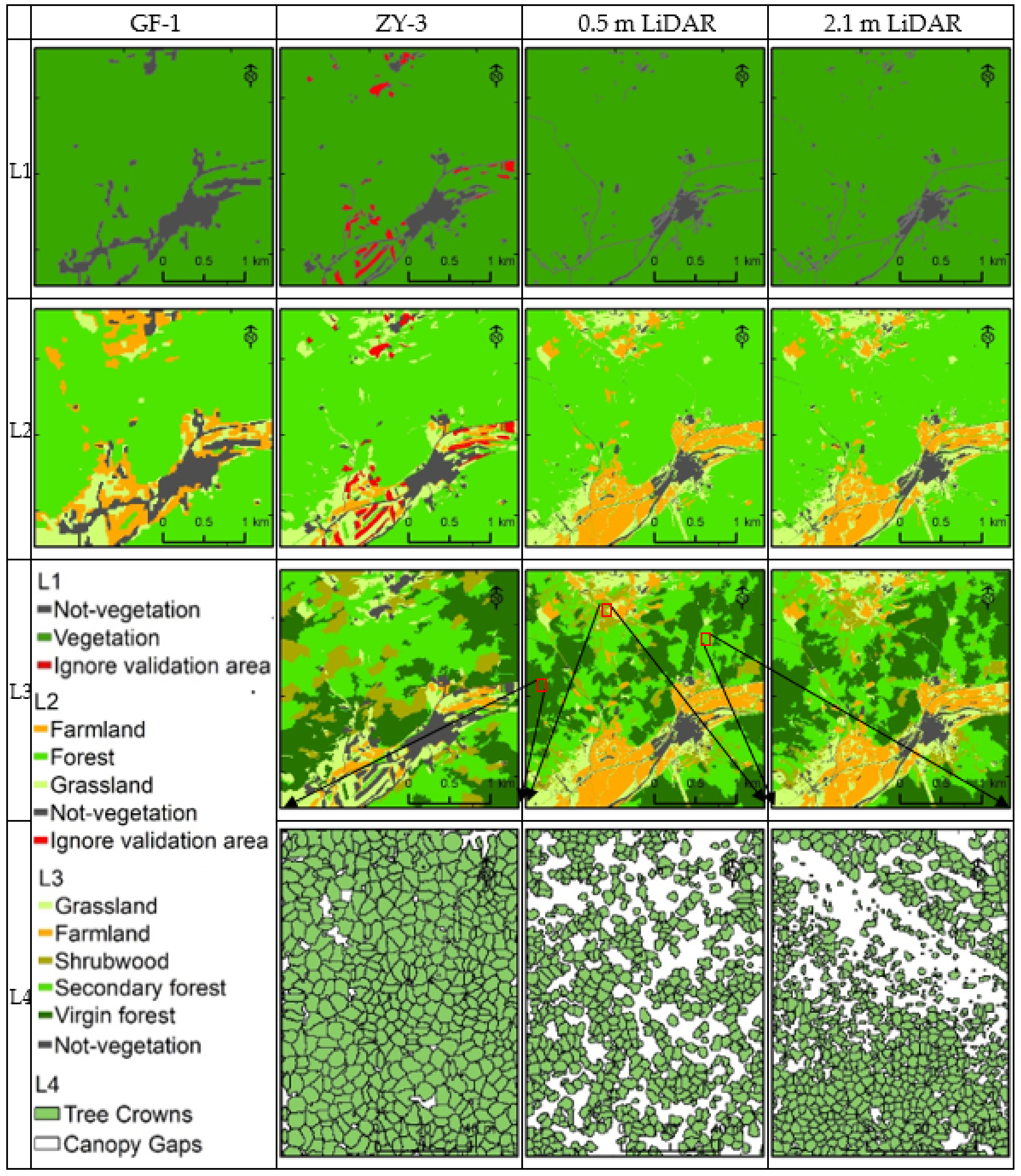
Figure 4.
Distribution of L1 (vegetation and non-vegetation), L2 (vegetation type), L3 (forest type) and L4 (canopy and canopy gaps).
Figure 4.
Distribution of L1 (vegetation and non-vegetation), L2 (vegetation type), L3 (forest type) and L4 (canopy and canopy gaps).

Figure 5.
Total accuracy comparison results. (a) Average total classification accuracy of four data sources; (b) total classification accuracy of four levels and (c) proportion of area of each category of L1 to L3 layers to the area of the parent class.
Figure 5.
Total accuracy comparison results. (a) Average total classification accuracy of four data sources; (b) total classification accuracy of four levels and (c) proportion of area of each category of L1 to L3 layers to the area of the parent class.


Table 1.
Multi-source remote sensing image dataset for vegetation type extraction.
| Image Type | Sensor | Image Time | Cell Size | Spectral Band (nm) | Geometric Attribute |
|---|---|---|---|---|---|
| GF-1 | WFV | 16 September 2015 | 16 m | Blue (0.45–0.52), | Level2A |
| Green (0.52–0.59), | |||||
| Red (0.63–0.69), | |||||
| Near infrared (0.77–0.89) | |||||
| ZY-3 | Multispectral camera | 16 September 2014 | 2.1 m | Blue (0.45–0.52), | Level3A |
| Green (0.52–0.59), | |||||
| Red (0.63–0.69), | |||||
| Near infrared (0.77–0.89), | |||||
| Full color (0.50–0.80) | |||||
| CHM | Riegl LMS-Q680i | 14–15 September 2015 | 0.5 m/2.1 m | — | Geographic registration |
| FCC | |||||
| DOM | Digi CAM-60 | 14–15 September 2015 | 0.2 m | RGB color | Geographic registration |
Table 2.
Four layers of image object processing and classification rule set.
| Level | Category | GF-1 | ZY-3 | 2.1 m LiDAR | 0.5 m LiDAR |
|---|---|---|---|---|---|
| L1 | Object domain | Multiresolution seg. (SP:0.2, S:0.001, C:0.2) | Multiresolution seg. (SP:1.5, S:0.0005, C:0.5) | Multiresolution seg. (SP:2, S:0.001, C:0.9, w:2CHM-3FCC) | Multiresolution seg. (SP:30, S:0.001, C:0.5, w:2CHM-3FCC) |
| Vegetation | FDI ≥ 0.16 or NDVI ≥ 1 | FDI ≥ 0.09 or NDVI ≥ 0.8 | Mean FCC ≥ 0.16 | Mean FCC ≥ 0.16 | |
| Non-vegetation | Non-vegetation object | Non-vegetation object | Non-vegetation object | Non-vegetation object | |
| L2 | Object domain | L1 layer vegetation object | L1 layer vegetation object | After the L1 layer vegetation objects are merged Contrast split seg. (CHM: edge ratio, 0.07~1, add 0.05) | After the L1 layer vegetation objects are merged Contrast split seg. (CHM: edge ratio, 0.07~1, add 0.05) |
| Forest | SVM, SNN, CART | SVM, SNN, CART | Mean CHM ≥ 0.08 | Mean CHM ≥ 0.08 | |
| Farmland | Cross-L3 interaction classification | Cross-L3 interaction classification | |||
| Grassland | Non-forest, farmland objects | Non-forest, farmland objects | |||
| L3 | Object domain | — | After the L2 layer forest objects are merged Multiresolution seg. (SP:5, S:0.001, C:0.8, w:1PCA1) | After the L2 layer forest objects are merged Multiresolution seg. (SP:6, S:0.001, C:0.8, w:1CHM-1FCC) | After the L2 layer forest objects are merged Multiresolution seg. (SP:40, S:0.001, C:0.8, w:1CHM-1FCC) |
| Low bush | Mean NIR ≤ 0.24 and Std. deviation NIR ≥ 0.032 | Mean CHM ≤ 0.3 | Mean CHM ≤ 0.3 | ||
| Original forest | Mean NIR ≥ 0.24 | Mean CHM > 0.55 and Std. deviation CHM < 0.14 | Mean CHM > 0.55 and Std.deviation CHM < 0.14 | ||
| Secondary forest | Mean NIR ≤ 0.24 and Std.deviation NIR < 0.032 | 0.3 < Mean CHM ≤ 0.55 or Std.deviation CHM ≥ 0.14 | 0.3 < Mean CHM ≤ 0.55 or Std.deviation CHM ≥ 0.14 | ||
| L4 | forest type | Shrub | Original forest | Secondary forest | |
| Object domain | L3 layer object Chessboard seg.:1 | L3 layer object Chessboard seg.:1 | L3 layer object Chessboard seg.:1 | ||
| Canopy gap | — | Mean CHM ≤ 0.04 | Mean CHM ≤ 0.48 | Mean CHM ≤ 0.48 | |
| Single-tree canopy | The local maximum point of CHM in the range of 3 m is in accordance with Mean CHM > 0.04 and Existence of Gaps (0) ≠ 1 as seeds; Growth was performed in regions with Ratio to neighbor < 1.5 until Area > 15 m2 or Length/Width > 2.3 | The local maximum point of CHM in the range of 3 m is in accordance with Mean CHM > 0.48 and Existence of Gaps (0) ≠ 1 as seeds; Growth was performed in regions with Ratio to neighbor < 1.5 until Area > 30 m2 or Length/Width > 2.3 | The local maximum point of CHM in the range of 4 m is in accordance with Mean CHM > 0.48 and Existence of Gaps (0) ≠ 1 as seeds; Growth was performed in regions with Ratio to neighbor < 1.5 until Area > 25 m2 or Length/Width > 2.3 |
Note: SP: scale parameter, S: shape, C: compactness, w: layer weight, FDI: forest discrimination index, NDVI: normalized difference vegetation index, CHM: canopy height model, FCC: fractional canopy cover, NIR: near-infrared, PCA1: first principal component.
Table 3.
Statistical summary of hierarchical classification accuracy data based on area (unit: %).
| Level | Category | GF-1 | ZY-3 | 2.1 m LiDAR | 0.5 m LiDAR | |||||||||||||
|---|---|---|---|---|---|---|---|---|---|---|---|---|---|---|---|---|---|---|
| P A | U A | T A | O A | P A | U A | T A | O A | P A | U A | T A | O A | P A | U A | T A | O A | |||
| L1 level (L1) | Vegetation | 89 | 99 | 88 | 88 | 96 | 98 | 94 | 94 | 99 | 99 | 97 | 97 | 99 | 99 | 98 | 98 | |
| Non-vegetation | 80 | 29 | 27 | 71 | 50 | 42 | 81 | 76 | 64 | 81 | 84 | 71 | ||||||
| L2 level (L2) | Forest | SVM | 90 | 92 | 84 | 67 | 88 | 91 | 81 | 72 | 96 | 98 | 94 | 89 | 98 | 98 | 96 | 93 |
| SNN | 89 | 94 | 84 | 69 | 95 | 87 | 83 | 73 | ||||||||||
| CART | 88 | 95 | 84 | 66 | 87 | 90 | 80 | 72 | ||||||||||
| Grassland | SVM | 12 | 27 | 9 | 67 | 66 | 37 | 31 | 72 | 84 | 68 | 60 | 87 | 81 | 72 | |||
| SNN | 36 | 37 | 22 | 69 | 47 | 36 | 26 | 73 | ||||||||||
| CART | 16 | 24 | 10 | 66 | 35 | 33 | 20 | 72 | ||||||||||
| Farmland | SVM | 66 | 46 | 37 | 67 | 27 | 70 | 24 | 72 | 77 | 89 | 70 | 89 | 93 | 83 | |||
| SNN | 66 | 53 | 42 | 69 | 20 | 79 | 18 | 73 | ||||||||||
| CART | 65 | 43 | 35 | 66 | 65 | 59 | 45 | 72 | ||||||||||
| L3 level (L3) | Original forest | — | — | — | — | 26 | 19 | 13 | 25 | 57 | 69 | 46 | 68 | 79 | 71 | 60 | 80 | |
| Secondary forest | — | — | — | 22 | 27 | 14 | 80 | 64 | 55 | 81 | 82 | 69 | ||||||
| shrub | — | — | — | 33 | 38 | 21 | 65 | 88 | 59 | 81 | 91 | 75 | ||||||
| L4 level (L4) | Original forest | Single-tree canopy | — | — | — | — | — | — | — | — | — | — | — | — | — | — | 83 | 66 |
| Canopy gaps | — | — | — | — | — | — | — | — | — | 16 | 38 | 13 | ||||||
| Secondary forest | Single-tree canopy | — | — | — | — | — | — | — | — | — | — | — | — | — | — | 63 | 70 | |
| Canopy gaps | — | — | — | — | — | — | — | — | — | 82 | 81 | 68 | ||||||
| Shrub | Single-tree canopy | — | — | — | — | — | — | — | — | — | — | — | — | — | — | 72 | 71 | |
| Canopy gaps | — | — | — | — | — | — | — | — | — | 83 | 80 | 67 | ||||||
Note: PA: producer accuracy, UA: user accuracy, OA: total classification of single class, TA: overall accuracy of this layer, SVM: support vector machine classifier, SNN: standard nearest neighbor classifier, CART: classification regression tree classifier.
Publisher’s Note: MDPI stays neutral with regard to jurisdictional claims in published maps and institutional affiliations. |
© 2020 by the authors. Licensee MDPI, Basel, Switzerland. This article is an open access article distributed under the terms and conditions of the Creative Commons Attribution (CC BY) license (http://creativecommons.org/licenses/by/4.0/).
Share and Cite
MDPI and ACS Style
Mao, X.; Deng, Y.; Zhu, L.; Yao, Y. Hierarchical Geographic Object-Based Vegetation Type Extraction Based on Multi-Source Remote Sensing Data. Forests 2020, 11, 1271. https://doi.org/10.3390/f11121271
AMA Style
Mao X, Deng Y, Zhu L, Yao Y. Hierarchical Geographic Object-Based Vegetation Type Extraction Based on Multi-Source Remote Sensing Data. Forests. 2020; 11(12):1271. https://doi.org/10.3390/f11121271
Chicago/Turabian StyleMao, Xuegang, Yueqing Deng, Liang Zhu, and Yao Yao. 2020. "Hierarchical Geographic Object-Based Vegetation Type Extraction Based on Multi-Source Remote Sensing Data" Forests 11, no. 12: 1271. https://doi.org/10.3390/f11121271
Note that from the first issue of 2016, this journal uses article numbers instead of page numbers. See further details here.