Detecting Harvest Events in Plantation Forest Using Sentinel-1 and -2 Data via Google Earth Engine


1
Department of Geography, University of the Free State, Phuthaditjhaba 9869, South Africa
2
School of Agricultural, Earth and Environmental Sciences, University of KwaZulu-Natal, Westville Campus, Durban 4000, South Africa
3
Department of Geography and Environmental Studies, University of Zululand, KwaDlangezwa 3886, South Africa
*
Author to whom correspondence should be addressed.
Forests 2020, 11(12), 1283; https://doi.org/10.3390/f11121283
Submission received: 17 August 2020
/
Revised: 25 November 2020
/
Accepted: 26 November 2020
/
Published: 29 November 2020
(This article belongs to the Special Issue Monitoring and Assessing Forest Attributes Based on Remote Sensing Technology)
Abstract
:South Africa is reported to experience timber shortages as a result of growing timber demands and pulp production, coupled with the government’s reluctance to grant new forestry permits. Rampant timber theft in the country makes these circumstances worse. The emergence of cloud-based platforms, such as Google Earth Engine (GEE), has greatly improved the accessibility and usability of high spatial and temporal Sentinel-1 and -2 data, especially in data-poor countries that lack high-performance computing systems for forest monitoring. Here, we demonstrate the potential of these resources for forest harvest detection. The results showed that Sentinel-1 data are efficient in detecting clear-cut events; both VH and VV backscatter signals decline sharply in accordance with clear-cutting and increase again when forest biomass increases. When correlated with highly responsive NDII, the VH and VV signals reached the best accuracies of 0.79 and 0.83, whereas the SWIR1 achieved –0.91. A Random Forest (RF) algorithm based on Sentinel-2 data also achieved over 90% accuracies for classifying harvested and forested areas. Overall, our study presents a cost-effective method for mapping clear-cut events in an economically important forestry area of South Africa while using GEE resources.
Keywords:
forest; Sentinel-1; Sentinel-2; harvest; RF classification; remote sensing; Google Earth Engine1. Introduction
Commercial forestry is a primary and widespread land-use activity along the eastern seaboard of South Africa, with nearly 1.2 million hectares being devoted to timber production [1]. The establishment of these plantations has been repeatedly hampered by disturbances, such as forest fires [2], the outbreak of insect pests and disease [3], invasive alien plants [4], and drought [5,6]. Additionally, forest land-use modification that arises from harvesting operations has become the main source of contemporary forest disturbance [7]. Because of the increase in the demand for timber and pulp products, combined with government’s reluctance to grant new forestry permits, South Africa is currently facing timber shortages [8], which are, in part, further heightened by rampant timber theft [9]. Similar concerns about the effects of illegal logging and trade in timber prompted the European Commission in order to adopt the EU Action Plan for Forest Law Enforcement, Governance and Trade (FLEGT) in 2003—an effort that is intended to improve the legitimacy of the production and sale of timber [10]. This plan entails a variety of measures to timber producing countries, such as South Africa, which include promoting public procurement policies, safeguards for financing and investment, addressing the problem of conflict timber, and so on [11]. In this regard, the mapping of forest change provides insight into timber procurement potential and future forest growth patterns [12], as well as risks that are associated with rapidly changing forest landscapes [13].
In the face of rapid and multiple forest changes, the stand- and landscape-level information that reveals disturbance patterns is particularly relevant for countries, such as South Africa, whose forestry resources contribute greatly to the economy. The planning and execution of timber harvesting to sustain or increase forest ecosystem services (that is, carbon stocks) prevail in the context of escalating forest disturbances [14] in order to meet forest management objectives [15]. While harvest operations are generally well known in advance by forest authorities, independent means for mapping are often pursued after the event [16]. In addition, the reality of timber theft has been a wake-up call and put forest managers under tremendous strain to aim for optimum production. In particular, the capacity of remotely sensed data to empower forest managers and communities to respond in time to unauthorized and other forest disturbances is increasingly recognized [17,18].
Remote sensing has emerged as the most practical and efficient means for extracting forest change information, with great temporal and thematic detail [19]. Consequently, numerous digital change detection methods have been developed in order to monitor forest disturbances [20], most of which involves bi-temporal image differencing procedures [21,22]. However, it should be noted that disturbances do not merely produce differences between conditions after time intervals, but rather a continuous process with varying degrees of occurrence [23]. For this reason, methods that are capable of continuously recording disturbance dynamics in a dense, remote-sensing time series have been developed [24], enabling the tracking of short- to long-term and partial to extreme disturbances [25], in ways that surpass traditional methods [26].
Ideally, near-real-time Earth observing platforms, such as AVHRR and MODIS, are desirable for time series analysis, but they are unavailable to record fine-scale alterations that are crucial for management requirements [27]. For example, MODIS misses up to 50% of the forest changes when compared to medium-resolution (30 m) Landsat data [28], and probably more as compared with 10-m Sentinel data. Persistent-cloud conditions also present a challenge for optical satellites, especially in tropical and sub-tropical regions. Instead, the all-weather Synthetic Aperture Radar (SAR) sensors overcome this difficulty by imaging surface features, irrespective of cloud conditions [29]. In forestry applications, microwave observations are increasingly becoming a preferred data source due to their sensitivity to forest-cover loss and growth stages [30]. However, the use of SAR in forest applications has not developed to the extent of optical platforms, partly because of the hitherto limited data processing capability [31]. The policy of making data freely available, which was introduced in 2008, unlocked access to records of satellite data from several space agencies and data suppliers such as NASA, the US Geological Survey and, more recently, the European Space Agency [15,32]. In order to support these resources, the Google Earth Engine (GEE) provides a cloud-computing platform to access massive, freely available, and pre-processed remotely sensed imagery [33], including the Sentinel-1 ground range detected (GRD) SAR and Sentinel-2 archive.
Various studies have demonstrated the use of SAR for characterizing forest disturbance with a high degree of success. For example, Salas et al. [34] detected the variability in normalized radar cross-sections under different forest conditions and noted higher L-band HH-backscatter on cleared forest than on established plantations. Santoro et al. [35] applied a simple detection algorithm with the ALOS-2 PALSAR and achieved high accuracies (>50%) for clear-cut detection, despite the shortcomings in terms of delineation. Accordingly, the L-band SAR observations are currently available from the ALOS-2 PALSA-2 mission that was launched in 2014 [36], but only a few images are available each year for most tropical regions, and the costs charged prohibit their operational use [30]. Moreover, the automated monitoring systems of harvest events that capture their spatiotemporal variability are essential for timber management, and they require the SAR backscatter that is sensitive to forest cover with consistent observations over time [35].
The recently launched Sentinel-1 satellite offers great possibilities for monitoring forest resources with readily available time series data [37], comprising C-band with a much superior temporal coverage (6–12 days) when compared with previous SAR constellations [38]. Sentinel-1 has already displayed a high ability for monitoring forest applications, such as forest classification [39], forest cover mapping [40], burnt forested areas [41], forest logging [42], and deforestation [30]. In this paper, we further evaluate the utility of the weather-insensitive Sentinel-1 C-band, together with Sentinel-2 multispectral imagery, for monitoring forest harvesting events in KwaMbonambi, South Africa. Despite their potential for forest monitoring, only few studies have utilized these resources in order to detect clear-cut harvest events and, even are limited by exploring the GEE environment. Here, we demonstrate how to reconstruct high-density Sentinel-1 C-band time series in the process classify harvest events in planted forests while using Sentinel-2 within a cloud-based GEE platform and, consequently, stress the value of these resources for this purpose. We then compare the performance of Sentinel-1 with Landsat-8 data in detecting harvest events, as recommended by [43]. Finally, we illustrate how our results serve to identify harvest events in planted forests and how they could efficiently help monitor related disturbances, such as unauthorized harvesting and deforestation in different forest types.
2. Materials and Methods
2.1. Study Area
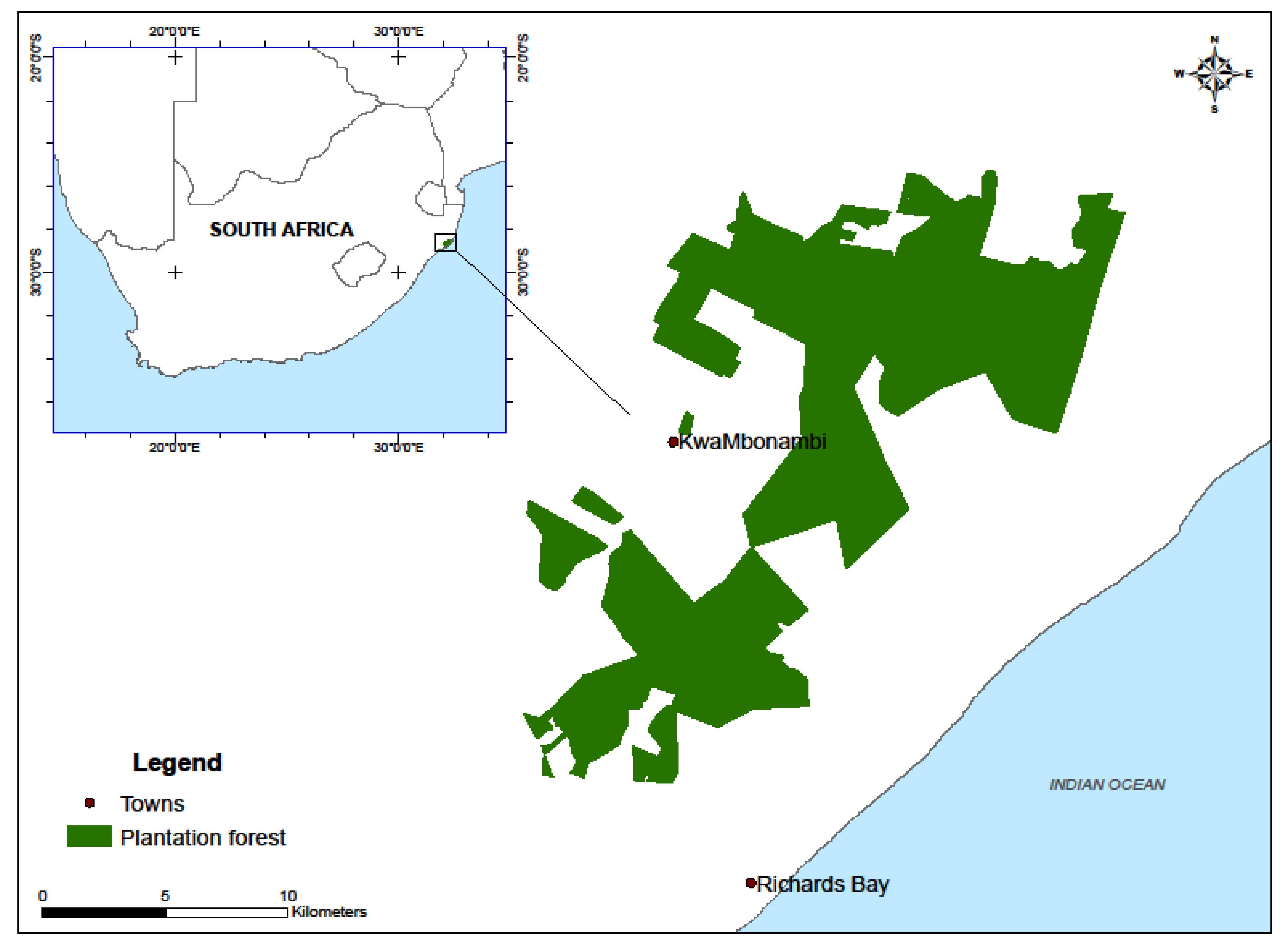
The study was performed in the KwaMbonambi plantation forests, which are located along the eastern seaboard of South Africa, 30 km northeast of Richards Bay (Figure 1). They are dominated by even-aged Eucalyptus plantations of almost 40,000 ha, which are managed by Sappi, a large South African pulp and paper company. This area is representative of frequently harvested forests and it provides an ideal testing location. The growing stock mainly comprises 6–14-year-old Eucalyptus grandis (E. grandis), E. grandis × Eucalyptus camaldulensis (E. gxc), and E. grandis × Eucalyptus urophylla (E. gxu) hybrid clones. The stands are fairly uniform regarding canopy cover with tree density established at 1667 trees ha–1. It is typical of the northern KwaZulu-Natal forestry region, which is subject to notable forest disturbances, such as fire and insect pest outbreaks. A subtropical climate characterizes the area, and the mean annual temperature is 22 °C [44]. The area receives an annual rainfall averaging 1200 mm, which is highly seasonal and peaks between November and February [45]; the potential evapotranspiration is 1772 mm per year [46]. The landscape of KwaMbonambi is flat and it consists of Quaternary alluvial sediments of clay sands of aeolian deposits [47] and soil with varying levels of organic matter [48], at mean elevation of 74 m above sea level. The high penetrability of the soils permits rapid leaching of soil nutrients due to the high rainfall in this region [47]. These conditions are favorable for fast-growing Eucalyptus plantations [49].
We used the vector polygons of known clear-cut compartments from Sappi, comprising felled date, areal extent, stand age classes, and forest types, in order to validate the clear-cut mapping results. These compartments were used to test whether high-density, readily available Sentinel-1 and -2 data can serve to detect harvest events with accuracies that are comparable with those acquired through forest inventories. Table 1 specifies the characteristics of the selected stands against which the competence of Sentinel-1 and -2 data were tested to detect clear-cut harvesting. We studied similar forest species (E. gxu) to compare, because Dostálová et al. [40] attributed differences in microwave backscatter variations to forest type and structure, as can be seen from the table.
2.2. Satellite Data
All 110 available Sentinel-1, C-band SAR dense time series images, covering the KwaMbonambi area between June 2015 to December 2018, were used in order to detect clear-cut harvest events. The images were acquired and preprocessed by the GEE team while using the Sentinel-1 toolbox and available at no charge from the Google Earth Engine (GEE) cloud environment as image collection. The images were collected in Interferometric Wide Swath (IW, 250 km swath width) providing VV (Vertical transmit–Vertical receive) and VH (Vertical transmit–Horizontal receive) polarizations. This 10-m resolution, all-weather imagery with a 6–12-day revisit cycle was already processed at high-resolution Level-1 GRD level, which includes radiometric, geometric corrections and orthorectification [50]. We further applied the speckle filter using the JavaScript code editor in the GEE environment to reduce the speckle effect. As noted by Mermoz et al. [51], this filter produces images with reduced speckle effects, multi-temporal and multi-polarized (VH and VV) products, and are expressed, as follows:
where Ik(υ) is the radar intensity of output image k at pixel position υ, Ii(υ) is the radar intensity of the input image i, is the local average intensity of the input image i (window size of 7 × 7), and N is the number of images.
We also used Sentinel-2 Level-1C product representing Top of Atmosphere (TOA) reflectance for classification, again obtained and processed from the GEE environment. The spectrally sensitive Sentinel-2 is being increasingly utilized for various applications because of its high spatial (10-m) and temporal (3–5 days) resolutions.
We followed Nagler et al. [52] by using the Landsat-8-derived (L1 terrain corrected at TOA) normalized difference vegetation index (NDVI) and the normalized difference infrared index (NDII) values as references in order to evaluate the performance of Sentinel-1. In the region studied, Landsat data are impaired by data gaps due to persistent cloud cover. We then employed the spline interpolation to fit a cubic spline to each missing NDVI and NDII value over the time series, while using the R statistical package ‘spline’. Cubic spline interpolation is widely used in order to generate a complete time series [53]. Because of different acquisition dates, both NDVI and NDII as well as Sentinel-1 profiles were averaged to represent monthly intervals, so that observations correspond with each other. Moreover, the use of SAR requires the removal of speckle and noise, which are efficiently reduced with monthly composites [41]. The vegetation indices were computed from top-of-atmosphere reflectance, using the following equations:
2.3. Background and the Use of the GEE Platform
The remote sensing of forests has reached the stage that enables scientists to expend their efforts on information generation, rather than data preparation [54]. This has been achieved through the emergence of a cloud-based GEE platform, a computing environment that provides easy access to a multi-petabyte ready-to-use satellite data archive [55]. It affords users superior computing power for processing and analyzing images without computational burden, and coupled with a high-performance, intrinsically parallel computation service. The GEE archive contains the complete Landsat data set as well as Sentinel-1 and Sentinel-2 images, and it also includes climate and other geophysical data sets [55]. The GEE can visualize the data, plot it in time series graphs, and the data can be downloaded for external processing.
2.4. GEE-Based Random Forest Classification
The GEE offers a variety of advanced machine learning classifiers for pixel-based classification that can be used for multi-temporal land use mapping [56]. Here, we implemented a Random Forest (RF; [57]) classifier for harvested and forested pixels’ separation, and more information can be obtained from (https://developers.google.com/earth-engine/classification). RF has gained wide popularity, because of its high accuracy and ability to process complex datasets and produce satisfactory results with large numbers of input classification bands and training points [57]. We employed RF based on Sentinel-2 imagery, because it is ideal to classify very small plantations [58]. Certainly, some spectral bands are more important than others for the classification, and it has been established that, when more spectral bands are included, the accuracy is improved until a certain threshold is reached [59]. Thus, all of the spectral bands in the Sentinel-2 imageries were selected to train the classifier (Table 2).
Reference data for training and validation comprised harvest records from Sappi management database, in the form of ArcMap shapefile polygons. The shapefiles contained fell dates, areal extent for each compartment, etc. Within GEE, Sentinel-2 TrueColor imagery corresponding to the fell dates were filtered and 60 points for each harvested and forested compartment were sampled throughout the studied area. Up to now, no literature stipulates the minimum number of training samples for machine learning algorithms, and because harvested compartments are clearly discernible from forested ones, we believed that 60 samples are ideal for this kind of classification. In order to produce robust classification results, the classification of Sentinel-2 images was run 1000 times by randomly selecting 50% of reference data from each class for training, and testing against the other 50% [58].
In classification, the accuracy assessment is the necessary step in evaluating the performance of algorithm used. We computed producer accuracy (PA), which is calculated by dividing the number of correctly classified pixels in each category by the number of “known” pixels to be of that category, the user’s accuracy (UA), which is computed by dividing the number of correctly classified pixels in each category by the total number of pixels that were classified in that category, and the overall accuracy (OA) that is calculated by dividing the sum of correctly classified pixels by the total number of sampled pixels.
2.5. Statistical Analysis
A Taylor diagram was exploited to establish the relationship between spectral indices and the Sentinel-1 backscatter signals. This is a single diagram that synchronously combines three statistical performance metrics: the Pearson correlation coefficient, root mean square difference (RMSD), and the standard deviation in a series of points on a polar plot [60]. The RMSD is a measure of the average error that is produced by a model and it is widely used to gauge overall model performance. However, it does not reveal the types or sources of the error, which would assist greatly in refining the models [61]. The RMSD is calculated as:
3. Results and Discussion
3.1. Spatial Patterns of VH and VV Backscatter over Clear-Cut Stands and the Classification
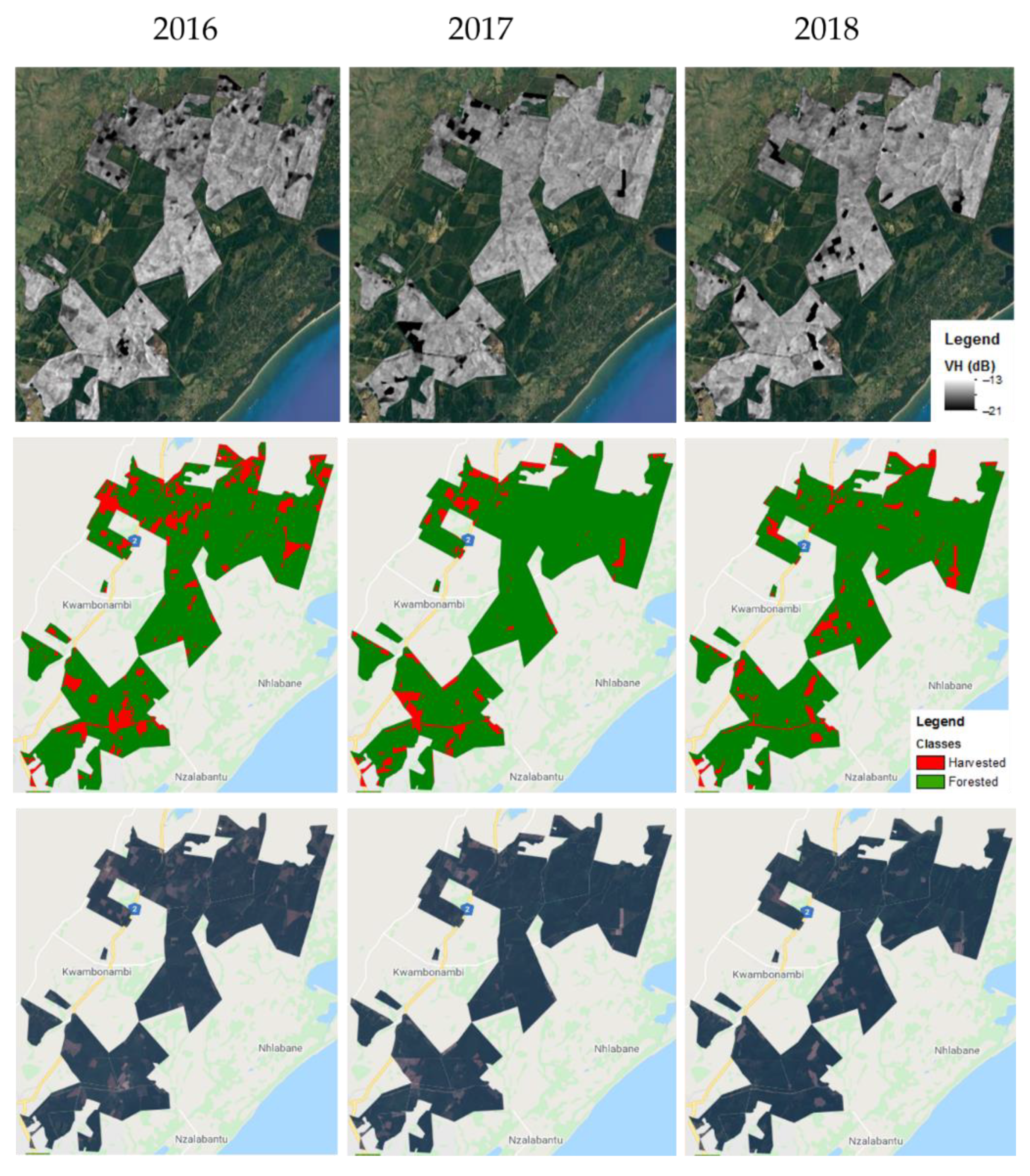
Figure 2 illustrates the comparisons between VH and VV backscatter signals and the field inventory record. It can be seen that both VH and VV bands detect the clear-cut events over the same area and time period. However, the VH appears fairly constant around −13 dB and −15 dB in uncut stands with a clear decline in backscatter signals over clear-cut stands reaching −21 dB. On the other hand, the VV bands seem to be more sensitive to various forest changes, as illustrated by the spread of weaker backscattered signals that were observed across the plantation, even over uncut stands. Despite this observation, the patterns of clear-cut stands are distinguishable from the VV backscatter, because they are dominant over clear-cut areas. Xu et al. [62] also noted that the VV band suffers from the complex effects of changes in the scattering mechanism. The variation in VV backscatter in 2016 is believed to be associated with the exceptional drought conditions reported by Xulu et al. [6]. Chatziantoniou et al. [63] noted that extreme drought affects the VV signal, because it reduces backscatter, which is sensitive to moisture conditions. The catastrophic character of the 2015–2016 drought led to widespread tree dieback in the Zululand forestry region [64]. This outcome appears to be illustrated by the extensive reduced VV backscatter over the uncut forest stands, as demonstrated in Figure 2.
The classification of harvested and forested compartments while using RF based on Sentinel-2 imagery successfully produced overall accuracies as high as 99% for all sampled years (Figure 2). The producer’s and user’s accuracies for both classes were consistently high, with each class attaining over 90%. Our results are consistent with Nomura and Mitchard [58], in their classification of a plantations in a complex forested landscape.
While both of the Sentinel-1 bands seem to be reactive to clear-cutting, and despite the small differences between them, the VV bands are seen to be slightly sensitive than the VH band. This observation is also consistent with greater correlation of VV band to highly responsive NDII (shown in the next sections).
We performed a time series analysis of VH and VV polarization indices and Landsat-derived NDVI and NDII (as reference) for each year separately over known harvested stands in the KwaMbonambi plantations in order to evaluate the effectiveness of Sentinel-1 backscattering to characterize clear-cut events. These sensors record different, yet related, forest attributes. In particular, VH and VV radar backscattering is highly correlated with fresh forest biomass, whereas NDVI is correlated with photosynthetic activity [31]. Given that clear-cutting is an extreme and abrupt forest change, and that sensors may yield signals with variations as a response to other forest dynamics, this study only considers the most significant breakpoints. We decided to only select three harvested compartments for each year to exemplify the behavior of Sentinel-1 and spectral bands when harvest events transpire, and the analysis is presented below.
3.2. Salient Trends for SAR and Vegetation Indices
3.2.1. Temporal Profile over Harvested Compartment in 2016
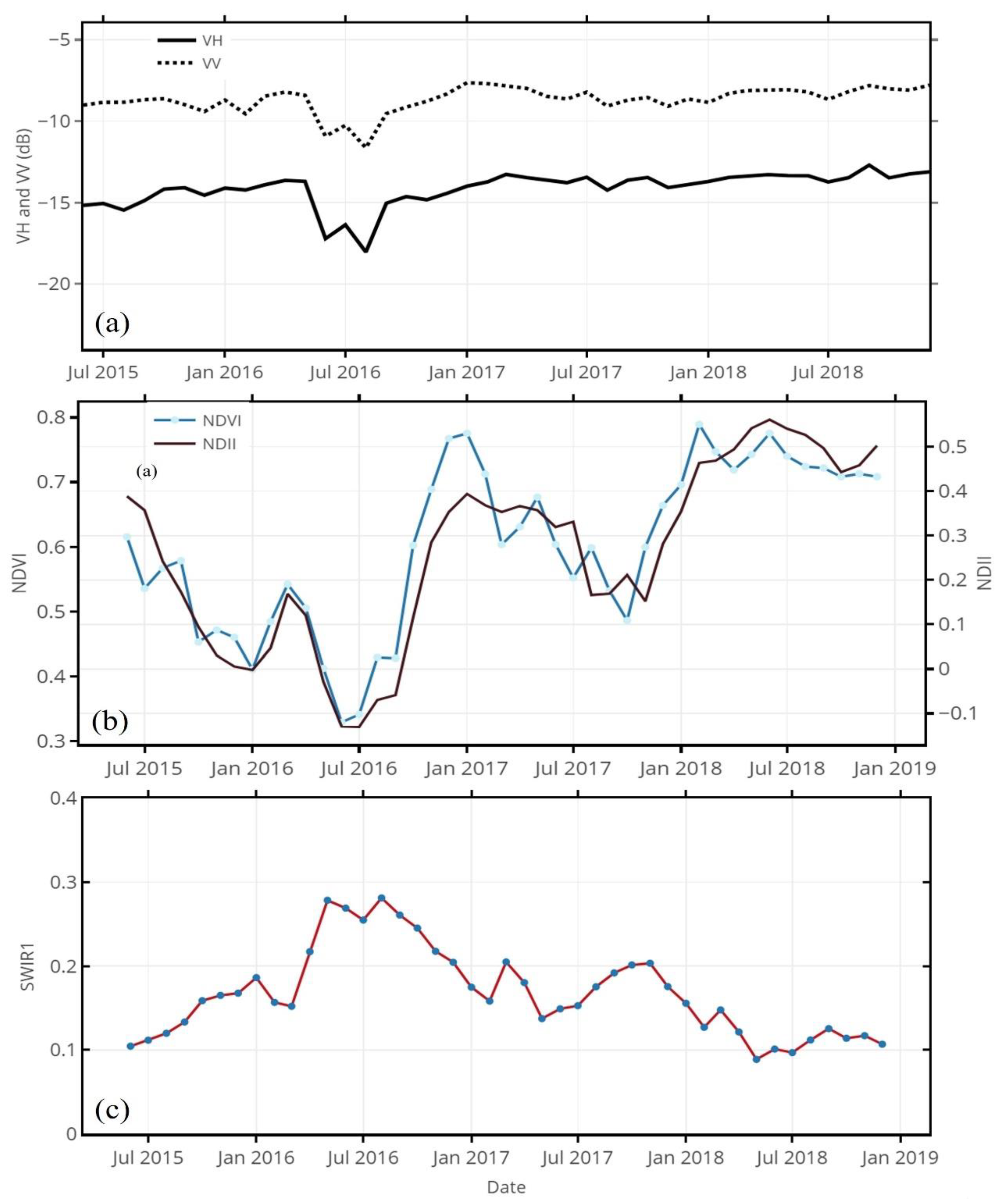
Figure 3 shows the temporal profiles of Sentinel-1 VH and VV backscatter (a), NDVI and NDII (b), and the shortwave infrared (SWIR1) (c) for the compartment harvested in 2016. The VH and VV polarized backscatter exhibited similar results for this compartment, generally with a virtually uniform pattern throughout the study period with the exception of a notable change in the middle of 2016. An abrupt reduction of 5 dB for VH (−13.7 to −18 dB) and 4 dB for VV (−8.4 to −11.6 dB) backscattering in June 2016 corresponds with a clear-cut harvest event, as confirmed by Sappi’s official inventory records. During this period, it appears, as expected from cleared forest, the VH polarization revealed much less backscattering than the VV signal. This observation is consistent with Nguyen et al. [65], who reported that VH polarized backscatter is generally less than VV, and that the backscattering coefficients for both polarizations progressively increase with tree growth over time. There was an obvious increase in the backscatter signal for both polarizations, corresponding with tree canopy increase after September 2016, reaching a peak of −8 dB (VV) and −13 dB (VH) around March 2017, when the forests reached maturity stage, as illustrated in Figure 3a. An equivalent finding was made by Macelloni et al. [66], who observed an increase in VH cross-polarized backscatter with increasing leaf area index (LAI) over planted forests in the Italian landscape. In a related study, Huang et al. [67] found that VH polarization is more efficient than VV for characterizing forest canopy dynamics, because it is less influenced by soil moisture. Nguyen et al. [66] attributed the reduced backscatter in the VV signal to the lower moisture content of trees during the harvest period; conversely, the VH signal seemed to be the least affected by this factor. Moreover, we agree with Karjalainen et al. [68] that VH polarization is better than VV to characterize the actual biomass variations in forests.
The NDII and NDVI values resembled the Sentinel-1 backscatter signals and declined during clear-cutting (Figure 3b). The NDII declined from 1.7 to −0.13 and recovered to 0.39 a few months later. The NDVI also decreased, from 0.54 to 0.32, after a clear-cut event and rose to 0.77 during the forest growth phase.
It is important to note the increase of the SWIR1 signal during clear-cutting. At this time, the SWIR1 rose from 0.15 to its highest maximum of 0.28 (Figure 3c). Indeed, clear-cutting is well-known to increase the reflectance in the SWIR1 band [69]. This is particularly so, because the SWIR1 band is sensitive to vegetation density [70]. Thus, as forest canopy complexity increases with time, reflectance in the SWIR1 decreases [71]. Our results are in harmony with this observation—the SWIR1 signal declines as the forest canopy matures. In a related study, Schroeder et al. [72] classified forest disturbances while using Landsat-derived vegetation indices and found the SWIR1 channel to be the most effective for distinguishing clear-cut harvests.
3.2.2. Temporal Profile over Harvested Compartment in 2017
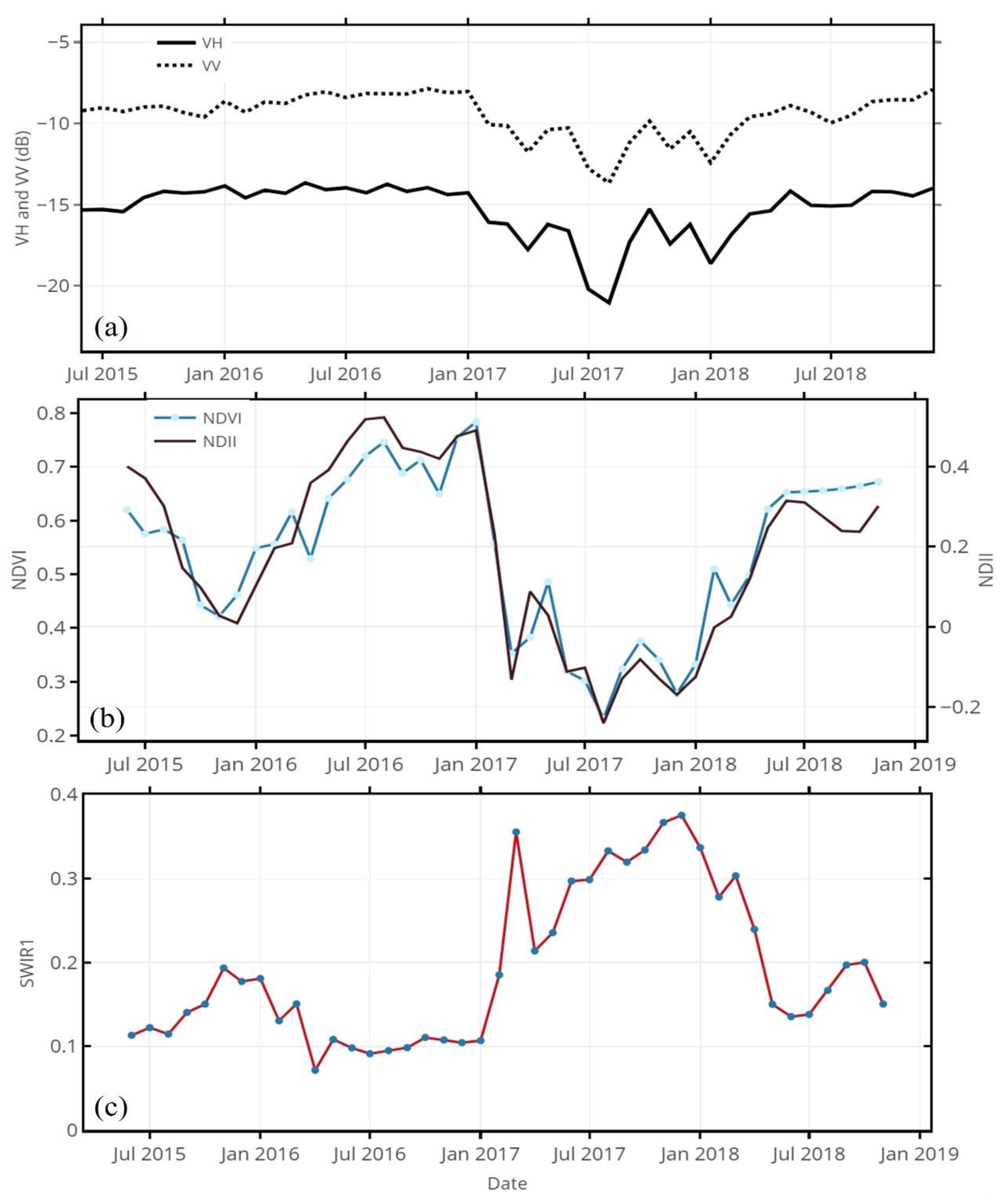
Figure 4 shows the VH and VV polarized signals over the compartment that was harvested in 2017. Both of the polarizations exhibited similar backscattering behavior to that of the above, this time decreasing in June 2017. Again, the decline in both polarization signals coincides with clear-cutting records from Sappi. In 2017, two disturbances were detected; the first in April led to reduced VH (−14.27 to −17.76 dB) and VV (−8.04 to −11.76 dB) backscatter signals. A further decrease in VH backscatter to −21.04 dB and to −13.66 dB for VV was witnessed in June (Figure 4a). During this period, a corresponding decrease in NDVI (0.78 to 0.35) and NDII (0.49 to −0.13) is noticeable around April and these values further declined in June to 0.23 and −0.24, respectively (Figure 4b). The increase in SWIR1 corresponds with reductions in the SAR backscatter signals and vegetation indices, as shown in Figure 4c. An initial increase in SWIR1 from 0.11 to 0.36 in April was followed by a further increase to 0.37 during a clear-cutting period.
3.2.3. Temporal Profile over Harvested Compartment in 2018
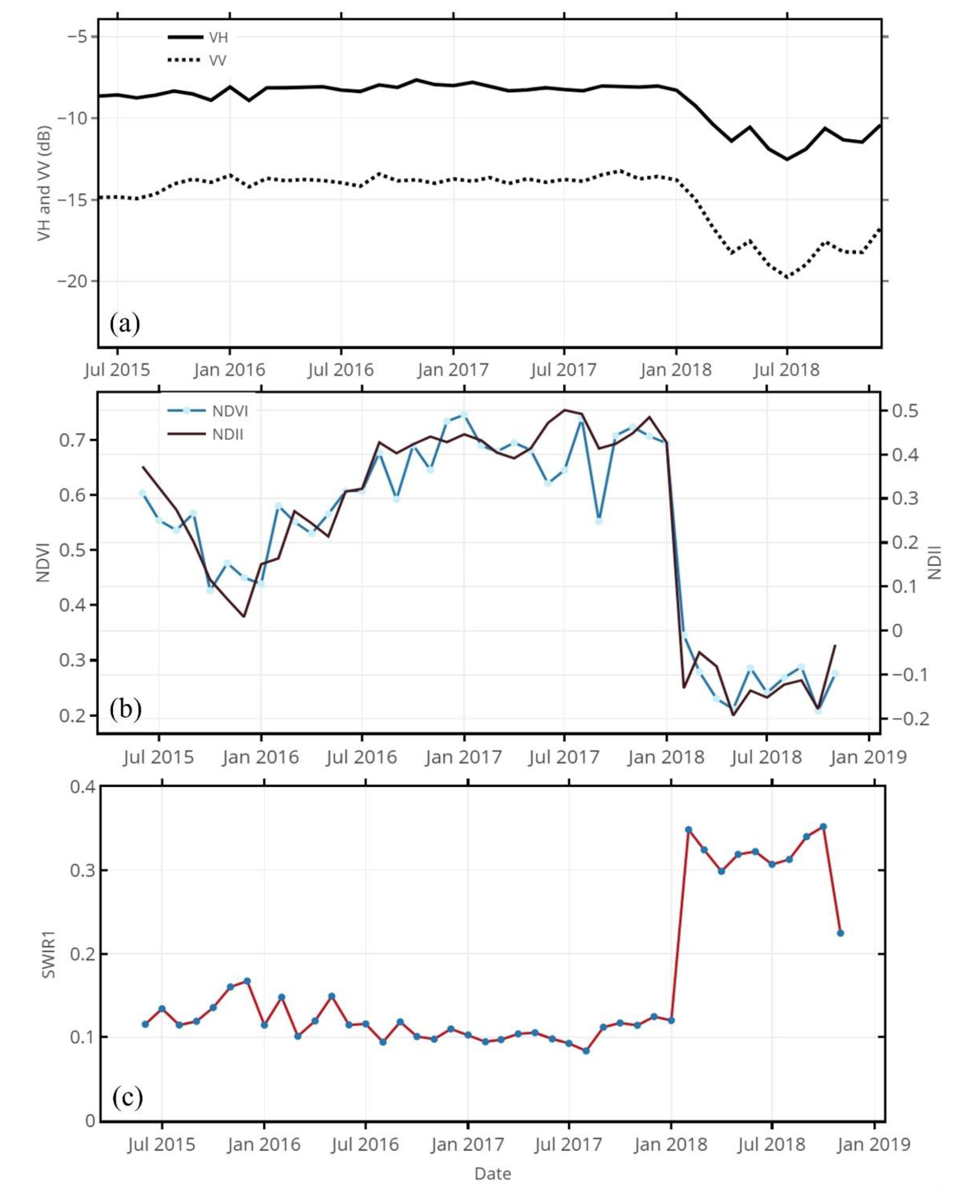
The pattern of VH and VV backscatter signals for the compartment that was harvested in 2018 was similar to that for 2016 and 2017 harvested compartments. The VH backscatter dropped from −13.81 dB in January 2018 to its lowest minimum (−19.82 dB) in July; the VV backscatter also declined, from −8.33 to −12.54 dB (Figure 5a). The NDVI value decreased from 0.72 to 0.21, whereas the NDII declined from 0.48 to −0.19 in the corresponding periods (Figure 5b). As expected, the SWIR1 increased from 0.11 to 0.34 over the time of the clear-cutting (Figure 5c).
Figure 3, Figure 4 and Figure 5 seems to indicate that Sentinel-1 can be an efficient weather-insensitive source from which clear-cutting activities are detectable. It is noteworthy that the Sentinel-1 backscatter appear to be responsive to various disturbances, but the dominant backscatter is obvious during clear-cutting. Similarly, the vegetation indices (NDVI and NDII) and the SWIR1 band showed a corresponding pattern to the Sentinel-1 backscatter signals, and these were useful in confirming the results. We now explain the relationship of these signals having described the temporal profiles of data derived from Sentinel-1 and Landsat-8.
3.3. Correlation between NDII Sentinel-1 and Other Vegetation Indices
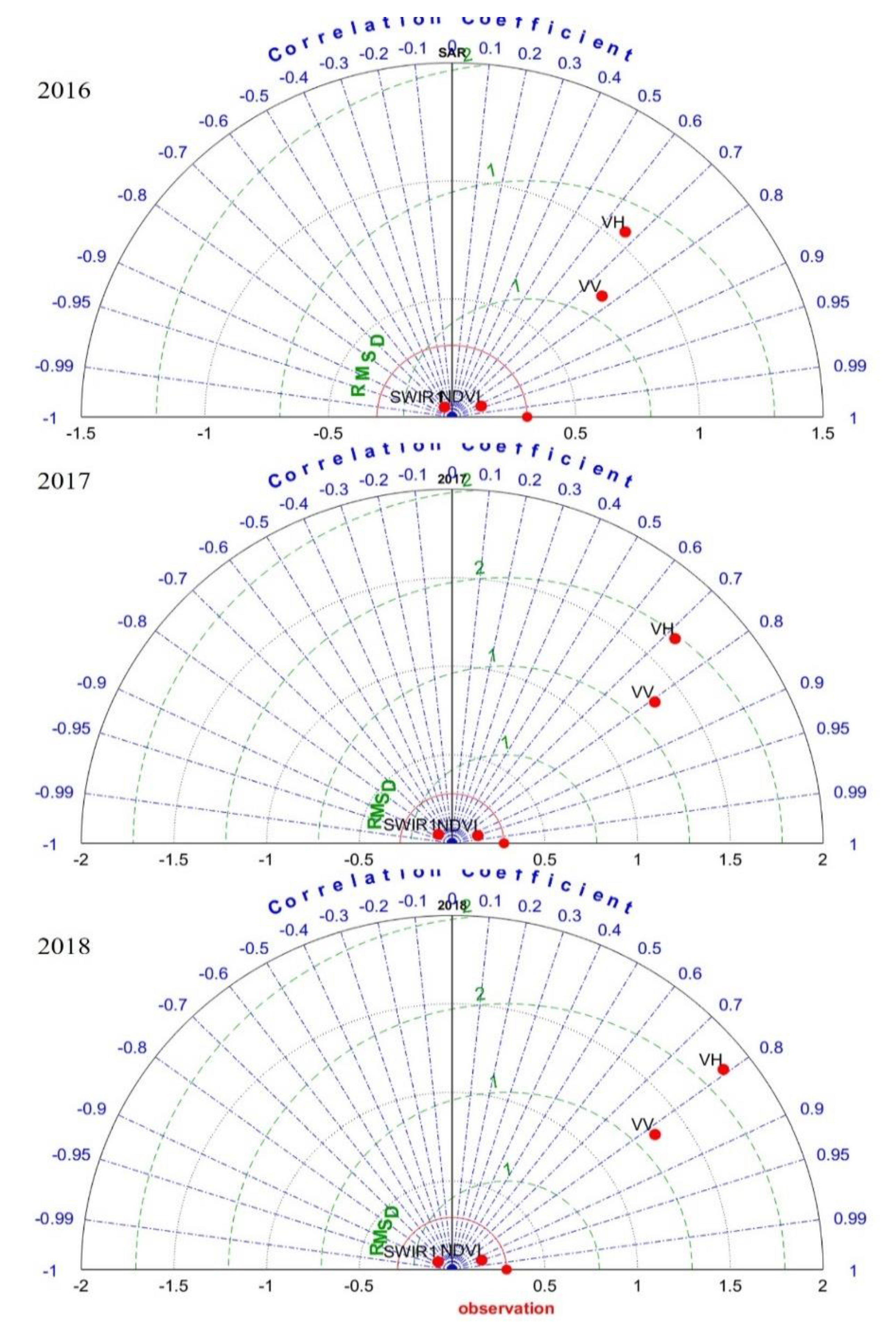
Given the greater sensitivity of NDII to clear-cutting events, we decided to use it as a reference variable in order to illustrate its relationship with microwave indices (VH and VV) as well as other vegetation criteria. For this purpose, Taylor diagrams [60] were computed in order to provide a graphical representation of how closely a pattern corresponds to the reference signal. The Taylor diagram is explanatory diagram that presents the visualization of the comparative strength of independent parameters to the actual target variable. In the Taylor diagram, the two different statistical metrics (i.e., correlation coefficients (R2) and standard deviations of each model) are used to quantify the comparability between the calculated data (e.g., models) and actual data. The distance from the reference point is a measure of the centered RMSD. The Taylor diagram is designed in such a way that it can graphically indicate which calculated data (or models) is most realistic. Figure 6 shows the corresponding Taylor diagram for the three different compartments, harvested in 2016, 2017, and 2018. The VV polarization was better correlated with NDII (compartment harvested in 2016, R2 = 0.78; compartment harvested in 2017, R2 = 0.81; compartment harvested in 2018, R2 = 0.82) than VH backscatter (2016 harvested compartment, R2 = 0.67; 2017 harvested compartment, R2 = 0.72; 2018 harvested compartment, R2 = 0.79). The values that correspond to these polarizations were grouped around the normalized standard deviation between 1.25 and 1.81, with VV showing less deviation from NDII than VH backscatter. The VV backscatter also had a smaller RMSD value (~1) than the VH signal (~2). Similar to those of Nagler et al. [52], these results reveal the good quality of both products that are derived from independent data sources.
As expected, the NDVI and SWIR1 results were more highly correlated with NDII than the Sentinel-1 bands; this was because the former were partly derived from similar bands to those of the NDII and also recorded by the same sensor. The NDVI values showed the greatest correlation (2016 harvested compartment, R2 = 0.93; 2017 harvested compartment, R2 = 0.95; 2018 harvested compartment, R2 = 0.96). Similarly, the SWIR1 results exhibited a strong negative correlation with NDII (2016 harvested compartment, R2 = −0.71; 2017 harvested compartment, R2 = −0.85; 2018 harvested compartment, R2 = −0.91), but a slightly smaller RMSD than that of the NDVI.
It is also important to note that the increasing water deficits increase the spectral reflectance in the SWIR1 region, and this largely influences the change in the vegetation values of indices that exploits this band, such as NDII [73]. The greater sensitivity of Sentinel-1 to moisture variations, particularly the VV band, could explain its higher correlation with the NDII.
4. Conclusions
Our study demonstrated the impressive capability of Sentinel-1 and -2 in order to detect and map clear-cut events in a complex commercial forestry area. The results showed high RF classification accuracies (99%) for harvested compartments based on Sentinel-2 data, which was consistent with Sentinel-1 backscatter. Our results also exhibited a similar temporal profile of VH and VV backscattering indices to those of NDVI and NDII; the respective signals were consistently relatively strong during the mature forest stage, but abruptly decreased after clear-cutting. In contrast, the SWIR1 band exhibited the opposite pattern with a sharp increase coinciding with clear-cutting, confirming reduced leaf water content prevailing at this time. When correlated with the highly responsive NDII, the VH and VV signals reached the best accuracies of 0.79 and 0.83, whereas the NDVI and SWIR1 achieved 0.96 and −0.91, respectively. The agreement between the VH and VV indices with NDII is satisfactory, because they are all derived from sensors that record different vegetation properties when compared to NDVI and SWIR1, which were not only recorded by the same sensor, but also implicitly contain NDII bands. Nevertheless, the VH and VV bands both consistently detected clear-cut events, the VH record indicated stable low backscattering over clear-cut stands, while the VV band appeared more sensitive, but it is affected by moisture stress and led to weaker backscattering signals even over uncut forest areas. Further research is desirable in exploring this method over broader areas and for different forest types. The responsiveness of the VV to moisture variations could also be tested in drought affected stands. We hope that our results will encourage remote sensing-based forest researchers in order to exploit the freely available GEE resources further and develop methodologies, in support of sustainable forest management, using high-density Sentinel-1 data to characterize forest changes, particularly in regions with poor image availability due to persistent cloud cover.
Author Contributions
Conceptualization, S.X., N.M., K.P. and M.G.; methodology, formal analysis, resources, writing of original draft, S.X., N.M., K.P. and M.G., and review and editing of final manuscript: S.X., N.M., K.P. and M.G. All authors have read and agreed to the published version of the manuscript.
Funding
This research was partly funded by the National Research Foundation of South Africa (grant number 114898).
Acknowledgments
Thanks to Graham Baker for manuscript editing and proof reading.
Conflicts of Interest
The authors declare no conflict of interest.
References
- Xulu, S.; Gebreslasie, M.T.; Peerbhay, K.Y. Remote sensing of forest health and vitality: A South African perspective. South. For. J. For. Sci. 2018, 81, 1–12. [Google Scholar] [CrossRef]
- DAFF (Department of Agriculture, Forestry and Fisheries). Report on Commercial Timber Resources and Primary Roundwood Processing in South Africa 2010/2011; Department of Agriculture, Forestry and Fisheries: Pretoria, South Africa, 2012.
- Lottering, R.; Mutanga, O. Optimizing the spatial resolution of WolrdView-2 pan-sharpened imagery for predicting levels of Gonipterus scutellatus defoliation in KwaZulu-Natal, South Africa. ISPRS J. Photogramm. Remote Sens. 2016, 112, 13–22. [Google Scholar] [CrossRef]
- Peerbhay, K.Y.; Mutanga, O.; Lottering, R.; Ismail, R. Mapping Solanum mauritianum plant invasions using WorldView-2 imagery and unsupervised random forests. Remote Sens. Environ. 2016, 182, 39–48. [Google Scholar] [CrossRef]
- Xulu, S.; Peerbhay, K.; Gebreslasie, M.; Ismail, R. Drought influence on forest plantations in Zululand, South Africa, using MODIS time series and climate data. Forests 2018, 9, 528. [Google Scholar] [CrossRef] [Green Version]
- Xulu, S.; Peerbhay, K.; Gebreslasie, M.; Ismail, R. Unsupervised clustering of forest response to drought stress in Zululand region, South Africa. Forests 2019, 10, 531. [Google Scholar] [CrossRef] [Green Version]
- Riitters, K.H.; Wickham, J.D.; O’neill, R.V.; Jones, K.B.; Smith, E.R.; Coulston, J.W.; Wade, T.G.; Smith, J.H. Fragmentation of continental United States forests. Ecosystems 2002, 5, 815–822. [Google Scholar] [CrossRef]
- FSA (Forestry South Africa). Planting Restrictions Cause Timber Shortage. Available online: http://www.forestry.co.za/planting-restrictions-cause-timber-shortage/ (accessed on 12 December 2018).
- Joubert, R. Theft Rampant in Timber Industry. 2013. Available online: https://www.farmersweekly.co.za/agri-news/south-africa/theft-rampant-in-timber-industry/ (accessed on 24 February 2019).
- Moral-Pajares, E.; Martínez-Alcalá, C.; Gallego-Valero, L.; Caviedes-Conde, Á.A. Transparency index of the supplying countries’ institutions and tree cover loss: Determining factors of EU timber imports? Forests 2020, 11, 1009. [Google Scholar] [CrossRef]
- FSA (Forestry South Africa). Illegal Logging and Forest Conformance Systems. Available online: http://saforestryonline.co.za/articles/illegal-logging-and-forest-conformance-systems/ (accessed on 20 October 2020).
- Saunders, M.R.; Arseneault, J.E. Potential yields and economic returns of natural disturbance-based silviculture: A case study from the Acadian Forest Ecosystem Research Program. J. For. 2013, 111, 175–185. [Google Scholar] [CrossRef]
- Hirschmugl, M.; Gallaun, H.; Dees, M.; Datta, P.; Deutscher, J.; Koutsias, N.; Schardt, M. Methods for mapping forest disturbance and degradation from optical earth observation data: A review. Curr. For. Rep. 2017, 3, 32–45. [Google Scholar] [CrossRef] [Green Version]
- Bradford, J.B.; Bell, D.M. A window of opportunity for climate-change adaptation: Easing tree mortality by reducing forest basal area. Front. Ecol. Environ. 2017, 15, 11–17. [Google Scholar] [CrossRef]
- Shimizu, K.; Ahmed, O.S.; Ponce-Hernandez, R.; Ota, T.; Win, Z.C.; Mizoue, N.; Yoshida, S. Attribution of disturbance agents to forest change using a Landsat time series in tropical seasonal forests in the Bago mountains, Myanmar. Forests 2017, 8, 218. [Google Scholar] [CrossRef]
- Rauste, Y.; Antropov, O.; Mutanen, T.; Häme, T. On clear-cut mapping with time-series of Sentinel-1 data in boreal forest. In Proceedings of the ESA Living Planet Symposium, Prague, Czech Republic, 9–13 May 2016; European Space Agency ESA: Paris, France, 2016. [Google Scholar]
- Wheeler, D.; Hammer, D.; Kraft, R.; Steele, A. Satellite-Based Forest Clearing Detection in the Brazilian Amazon: FORMA, DETER, and PRODES; World Resources Institute: Washington, DC, USA, 2014.
- Hansen, M.C.; Krylov, A.; Tyukavina, A.; Potapov, P.V.; Turubanova, S.; Zutta, B.; Ifo, S.; Margono, B.; Stolle, F.; Moore, R. Humid tropical forest disturbance alerts using Landsat data. Environ. Res. Lett. 2016, 11, 034008. [Google Scholar] [CrossRef]
- DeVries, B.; Pratihast, A.K.; Verbesselt, J.; Kooistra, L.; Herold, M. Characterizing forest change using community-based monitoring data and Landsat time series. PLoS ONE 2016, 11, e0147121. [Google Scholar] [CrossRef] [PubMed]
- Huang, C.; Goward, S.N.; Masek, J.G.; Thomas, N.; Zhu, Z.; Vogelmann, J.E. An automated approach for reconstructing recent forest disturbance history using dense Landsat time series stacks. Remote Sens. Environ. 2010, 114, 183–198. [Google Scholar] [CrossRef]
- Coppin, P.; Jonckheere, I.; Nackaerts, K.; Muys, B.; Lambin, E. Review article digital change detection methods in ecosystem monitoring: A review. Int. J. Remote Sens. 2004, 25, 1565–1596. [Google Scholar] [CrossRef]
- Healey, S.P.; Cohen, W.B.; Zhiqiang, Y.; Krankina, O.N. Comparison of Tasseled Cap-based Landsat data structures for use in forest disturbance detection. Remote Sens. Environ. 2005, 97, 301–310. [Google Scholar] [CrossRef]
- Kennedy, R.E.; Yang, Z.; Cohen, W.B. Detecting trends in forest disturbance and recovery using yearly Landsat time series: 1. LandTrendr—Temporal segmentation algorithms. Remote Sens. Environ. 2010, 114, 2897–2910. [Google Scholar] [CrossRef]
- Kuenzer, C.; Dech, S.; Wagner, W. Remote sensing time series revealing land surface dynamics: Status quo and the pathway ahead. In Remote Sensing Time Series; Springer: Cham, Switzerland, 2015; pp. 1–24. [Google Scholar]
- Hughes, M.; Kaylor, S.; Hayes, D. Patch-based forest change detection from Landsat time series. Forests 2017, 8, 166. [Google Scholar] [CrossRef]
- Senf, C.; Pflugmacher, D.; Hostert, P.; Seidl, R. Using Landsat time series for characterizing forest disturbance dynamics in the coupled human and natural systems of Central Europe. ISPRS J. Photogramm. Remote Sens. 2017, 130, 453–463. [Google Scholar] [CrossRef]
- Walker, J.J.; De Beurs, K.M.; Wynne, R.H.; Gao, F. Evaluation of Landsat and MODIS data fusion products for analysis of dryland forest phenology. Remote Sens. Environ. 2012, 117, 381–393. [Google Scholar] [CrossRef]
- Hansen, M.C.; Loveland, T.R. A review of large area monitoring of land cover change using Landsat data. Remote Sens. Environ. 2012, 122, 66–74. [Google Scholar] [CrossRef]
- Siegert, F.; Ruecker, G. Use of multitemporal ERS-2 SAR images for identification of burned scars in south-east Asian tropical rainforest. Int. J. Remote Sens. 2000, 21, 831–837. [Google Scholar] [CrossRef]
- Reiche, J.; Verhoeven, R.; Verbesselt, J.; Hamunyela, E.; Wielaard, N.; Herold, M. Characterizing tropical forest cover loss using dense Sentinel-1 data and active fire alerts. Remote Sens. 2018, 10, 777. [Google Scholar] [CrossRef] [Green Version]
- Veloso, A.; Mermoz, S.; Bouvet, A.; Le Toan, T.; Planells, M.; Dejoux, J.F.; Ceschia, E. Understanding the temporal behavior of crops using Sentinel-1 and Sentinel-2-like data for agricultural applications. Remote Sens. Environ. 2017, 199, 415–426. [Google Scholar] [CrossRef]
- Woodcock, C.E.; Allen, R.; Anderson, M.; Belward, A.; Bindschadler, R.; Cohen, W.; Gao, F.; Goward, S.N.; Helder, D.; Helmer, E.; et al. Free access to Landsat imagery. Science 2008, 320, 1011. [Google Scholar] [CrossRef]
- Shelestov, A.; Lavreniuk, M.; Kussul, N.; Novikov, A.; Skakun, S. Exploring google earth engine platform for big data processing: Classification of multi-temporal satellite imagery for crop mapping. Front Earth Sci. 2017, 5, 17. [Google Scholar] [CrossRef] [Green Version]
- Salas, W.A.; Ducey, M.J.; Rignot, E.; Skole, D. Assessment of JERS-1 SAR for monitoring secondary vegetation in Amazonia: I. Spatial and temporal variability in backscatter across a chrono-sequence of secondary vegetation stands in Rondonia. Int. J. Remote Sens. 2002, 23, 1357–1379. [Google Scholar] [CrossRef]
- Santoro, M.; Fransson, J.E.; Eriksson, L.E.; Ulander, L.M. Clear-cut detection in Swedish boreal forest using multi-temporal ALOS PALSAR backscatter data. IEEE J. Sel. Top. Appl. Earth Obs. Remote Sens. 2010, 3, 618–631. [Google Scholar] [CrossRef]
- Rosenqvist, A.; Shimada, M.; Suzuki, S.; Ohgushi, F.; Tadono, T.; Watanabe, M.; Tsuzuku, K.; Watanabe, T.; Kamijo, S.; Aoki, E. Operational performance of the ALOS global systematic acquisition strategy and observation plans for ALOS-2 PALSAR-2. Remote Sens. Environ. 2014, 55, 3–12. [Google Scholar] [CrossRef]
- Rüetschi, M.; Small, D.; Waser, L.T. Rapid detection of windthrows using Sentinel-1 C-band SAR data. Remote Sens. 2019, 11, 115. [Google Scholar] [CrossRef] [Green Version]
- Torbick, N.; Chowdhury, D.; Salas, W.; Qi, J. Monitoring rice agriculture across Myanmar using time series Sentinel-1 assisted by Landsat-8 and PALSAR-2. Remote Sens. 2017, 9, 119. [Google Scholar] [CrossRef] [Green Version]
- Balzter, H.; Cole, B.; Thiel, C.; Schmullius, C. Mapping CORINE land cover from Sentinel-1A SAR and SRTM digital elevation model data using random forests. Remote Sens. 2015, 7, 14876–14898. [Google Scholar] [CrossRef] [Green Version]
- Dostálová, A.; Wagner, W.; Milenković, M.; Hollaus, M. Annual seasonality in Sentinel-1 signal for forest mapping and forest type classification. Int. J. Remote Sens. 2018, 39, 7738–7760. [Google Scholar] [CrossRef]
- Verhegghen, A.; Eva, H.; Ceccherini, G.; Achard, F.; Gond, V.; Gourlet-Fleury, S.; Cerutti, P. The potential of Sentinel satellites for burnt area mapping and monitoring in the Congo Basin forests. Remote Sens. 2016, 8, 986. [Google Scholar] [CrossRef] [Green Version]
- Lei, Y.; Treuhaft, R.; Keller, M.; Dos-Santos, M.; Gonçalves, F.; Neumann, M. Quantification of selective logging in tropical forest with spaceborne SAR interferometry. Remote Sens. Environ. 2018, 211, 167–183. [Google Scholar] [CrossRef]
- Muro, J.; Canty, M.; Conradsen, K.; Hüttich, C.; Nielsen, A.; Skriver, H.; Remy, F.; Strauch, A.; Thonfeld, F.; Menz, G. Short-term change detection in wetlands using Sentinel-1 time series. Remote Sens. 2016, 8, 795. [Google Scholar] [CrossRef] [Green Version]
- DWAF (Department of Water Affairs and Forestry). Water Resource Protection and Assessment Policy Implementation Process. Resource Directed Measures for Protection of Water Resource: Methodology for the Determination of the Ecological Water Requirements for Estuaries; Department of Water Affairs and Forestry: Pretoria, South Africa, 2004. [Google Scholar]
- Dovey, S.B. Effects of clear felling and residue management on nutrient pools, productivity and sustainability in a clonal Eucalypt stand in South Africa. Ph.D. Thesis, Stellenbosch University, Stellenbosch, South Africa, 2012. [Google Scholar]
- Little, K.; Rolando, C. The impact of vegetation control on the establishment of pine at four sites in the summer rainfall region of South Africa. S. Afr. For. J. 2001, 192, 31–39. [Google Scholar] [CrossRef]
- Mucina, L.; Rutherford, M.C. The Vegetation of South Africa, Lesotho and Swaziland; South African National Biodiversity Institute: Pretoria, South Africa, 2006. [Google Scholar]
- Luvuno, L.; Kotze, D.; Kirkman, K. Long-term landscape changes in vegetation structure: Fire management in the wetlands of KwaMbonambi, South Africa. Afr. J. Aquat. Sci. 2016, 41, 279–288. [Google Scholar] [CrossRef]
- Lesch, W.; Scott, D.F. The response in water yield to the thinning of Pinus radiata, Pinus patula and Eucalyptus grandis plantations. For. Ecol. Manag. 1997, 99, 295–307. [Google Scholar] [CrossRef]
- ESA (European Space Agency). Sentinel-1 User Handbook; GMES-S1OP-EOPG-TN-13-0001; European Space Agency: Frascati, Italy, 2013; p. 80. Available online: https://sentinel.esa.int/documents/247904/685163/Sentinel-1_User_Handbook (accessed on 10 December 2018).
- Mermoz, S.; Le Toan, T. Forest disturbances and regrowth assessment using ALOS PALSAR data from 2007 to 2010 in Vietnam, Cambodia and Lao PDR. Remote Sens. 2016, 8, 217. [Google Scholar] [CrossRef] [Green Version]
- Nagler, T.; Rott, H.; Ripper, E.; Bippus, G.; Hetzenecker, M. Advancements for snowmelt monitoring by means of Sentinel-1 SAR. Remote Sens. 2016, 8, 348. [Google Scholar] [CrossRef] [Green Version]
- Halabisky, M.; Babcock, C.; Moskal, L. Harnessing the temporal dimension to improve object-based image analysis classification of wetlands. Remote Sens. 2018, 10, 1467. [Google Scholar] [CrossRef] [Green Version]
- Franklin, S.E.; Wulder, M.A. Remote sensing methods in medium spatial resolution satellite data land cover classification of large areas. Prog. Phys. Geogr. 2002, 26, 173–205. [Google Scholar] [CrossRef]
- Gorelick, N.; Hancher, M.; Dixon, M.; Ilyushchenko, S.; Thau, D.; Moore, R. Google Earth Engine: Planetary-scale geospatial analysis for everyone. Remote Sens. Environ. 2017, 202, 18–27. [Google Scholar] [CrossRef]
- Farda, N.M. Multi-temporal land use mapping of coastal wetlands area using machine learning in Google earth engine. In IOP Conference Series: Earth and Environmental Science; IOP Publishing: Bristol, UK, 2017; Volume 98, p. 012042. [Google Scholar]
- Breiman, L. Random forests. Mach. Learn. 2001, 45, 5–32. [Google Scholar] [CrossRef] [Green Version]
- Nomura, K.; Mitchard, E. More Than Meets the Eye: Using Sentinel-2 to Map Small Plantations in Complex Forest Landscapes. Remote Sens. 2018, 10, 1693. [Google Scholar] [CrossRef] [Green Version]
- Lee, J.S.H.; Wich, S.; Widayati, A.; Koh, L.P. Detecting industrial oil palm plantations on Landsat images with Google Earth Engine. Remote Sens. Appl. Soc. Environ. 2016, 4, 219–224. [Google Scholar] [CrossRef] [Green Version]
- Taylor, K.E. Summarizing multiple aspects of model performance in a single diagram. J. Geophys. Res. 2001, 106, 7183–7192. [Google Scholar] [CrossRef]
- Willmott, C.J. Some comments on the evaluation of model performance. Bull. Am. Meteorol. Soc. 1982, 63, 1309–1313. [Google Scholar] [CrossRef] [Green Version]
- Xu, Z.H.; Wang, R.; Ye, K.; Wang, W.; Quan, S.; Wei, M. Simultaneous range ambiguity mitigation and sidelobe reduction using orthogonal non-linear frequency modulated (ONLFM) signals for satellite SAR Imaging. Remote Sens. Lett. 2018, 9, 829–838. [Google Scholar] [CrossRef]
- Chatziantoniou, A.; Petropoulos, G.P.; Psomiadis, E. Co-orbital Sentinel 1 and 2 for LULC mapping with emphasis on wetlands in a Mediterranean setting based on machine learning. Remote Sens. 2017, 9, 1259. [Google Scholar] [CrossRef] [Green Version]
- Crous, C.J.; Greyling, I.; Wingfield, M.J. Dissimilar stem and leaf hydraulic traits suggest varying drought tolerance among co-occurring Eucalyptus grandis × E. urophylla clones. S. Afr. For. J. 2018, 80, 175–184. [Google Scholar] [CrossRef]
- Nguyen, D.B.; Gruber, A.; Wagner, W. Mapping rice extent and cropping scheme in the Mekong Delta using Sentinel-1A data. Remote Sens. Lett. 2016, 7, 1209–1218. [Google Scholar] [CrossRef]
- Macelloni, G.; Paloscia, S.; Pampaloni, P.; Marliani, F.; Gai, M. The relationship between the backscattering coefficient and the biomass of narrow and broad leaf crops. IEEE Trans. Geosci. Remote Sens. 2001, 39, 873–884. [Google Scholar] [CrossRef]
- Huang, X.; Ziniti, B.; Torbick, N.; Ducey, M.J. Assessment of forest above ground biomass estimation using multi-temporal C-band Sentinel-1 and polarimetric L-band PALSAR-2 data. Remote Sens. 2018, 10, 1424. [Google Scholar] [CrossRef] [Green Version]
- Karjalainen, M.; Kaartinen, H.; Hyyppä, J. Agricultural monitoring using Envisat alternating polarization SAR images. Photogramm. Eng. Remote Sensing. 2008, 74, 117–126. [Google Scholar] [CrossRef]
- White, J.C.; Saarinen, N.; Kankare, V.; Wulder, M.A.; Hermosilla, T.; Coops, N.C.; Pickell, P.D.; Holopainen, M.; Hyyppä, J.; Vastaranta, M. Confirmation of post-harvest spectral recovery from Landsat time series using measures of forest cover and height derived from airborne laser scanning data. Remote Sens. Environ. 2018, 216, 262–275. [Google Scholar] [CrossRef]
- Horler, D.N.H.; Ahern, F.J. Forestry information content of Thematic Mapper data. Int. J. Remote Sens. 1986, 7, 405–428. [Google Scholar] [CrossRef]
- Nilson, T.; Peterson, U. Age dependence of forest reflectance: Analysis of main driving factors. Remote Sens. Environ. 1994, 48, 319–331. [Google Scholar] [CrossRef]
- Schroeder, T.A.; Wulder, M.A.; Healey, S.P.; Moisen, G.G. Mapping wildfire and clearcut harvest disturbances in boreal forests with Landsat time series data. Remote Sens. Environ. 2011, 115, 1421–1433. [Google Scholar] [CrossRef]
- Eitel, J.U.; Gessler, P.E.; Smith, A.M.; Robberecht, R. Suitability of existing and novel spectral indices to remotely detect water stress in Populus spp. For. Ecol. Manag. 2006, 229, 170–182. [Google Scholar] [CrossRef]
Figure 1.
Location of KwaMbonambi plantation forest in the northeast coast of South Africa.

Figure 2.
The VH backscatter signals (top panels), Random Forest (RF) classification based on Sentinel-2 imagery (middle panels), and Sentinel-2 TrueColor (bottom panels) over KwaMbonambi forest (2016–2018) displaying harvested and forested compartments.
Figure 2.
The VH backscatter signals (top panels), Random Forest (RF) classification based on Sentinel-2 imagery (middle panels), and Sentinel-2 TrueColor (bottom panels) over KwaMbonambi forest (2016–2018) displaying harvested and forested compartments.

Figure 3.
Monthly mean profiles of VH and VV backscatter (a), normalized difference vegetation index (NDVI) and normalized difference infrared index (NDII) (b), and the SWIR1 (c) over harvested compartment in 2016.
Figure 3.
Monthly mean profiles of VH and VV backscatter (a), normalized difference vegetation index (NDVI) and normalized difference infrared index (NDII) (b), and the SWIR1 (c) over harvested compartment in 2016.

Figure 4.
Monthly mean profiles of VH and VV backscatter (a), NDVI and NDII (b), and the SWIR1 (c) signals over harvested compartment in 2017.
Figure 4.
Monthly mean profiles of VH and VV backscatter (a), NDVI and NDII (b), and the SWIR1 (c) signals over harvested compartment in 2017.

Figure 5.
Monthly mean profiles of VH and VV backscatter (a), NDVI and NDII (b), and the SWIR1 (c) signals over harvested compartment in 2018.
Figure 5.
Monthly mean profiles of VH and VV backscatter (a), NDVI and NDII (b), and the SWIR1 (c) signals over harvested compartment in 2018.

Figure 6.
Taylor diagrams showing the grouped correlation between NDII and VH, VV, NDVI, and SWIR1 for 2016–2018 harvested compartments.
Figure 6.
Taylor diagrams showing the grouped correlation between NDII and VH, VV, NDVI, and SWIR1 for 2016–2018 harvested compartments.


Table 1.
Characteristics of three selected compartments within the KwaMbonambi plantations harvested in 2016–2018.
Table 1.
Characteristics of three selected compartments within the KwaMbonambi plantations harvested in 2016–2018.
| Site Attributes | Harvested in 2016 | Harvested in 2017 | Harvested in 2018 |
|---|---|---|---|
| Species | E. gxu | E. gxu | E. gxu |
| Felled date | June 2016 | March 2017 | March 2018 |
| Coordinates | −28.58176, 32.19044 | −28.67932, 32.07779 | −28.66026, 32.12026 |
| Areal extent (ha) | 39 | 43 | 33 |
| Altitude (m.a.s.l) | 84 | 86 | 93 |
Table 2.
Spectral bands of the Sentinel-2 imagery.
| Spectral Band | Band Name | Wavelength | Spatial Resolution (m) |
|---|---|---|---|
| B1 | Coastal aerosol | 442.3–443.9 nm | 60 |
| B2 | Blue | 492.1–496.6 nm | 10 |
| B3 | Green | 559–560 nm | 10 |
| B4 | Red | 664.5–665 nm | 10 |
| B5 | Red edge 1 | 703.8–703.9 nm | 20 |
| B6 | Red edge 2 | 739.1–740.2 nm | 20 |
| B7 | Red edge 3 | 779.7–782.5 nm | 20 |
| B8 | NIR | 833–835.1 nm | 10 |
| B8A | NIR narrow | 864–864.8 nm | 20 |
| B9 | Water vapor | 943.2–945 nm | 60 |
| B10 | SWIR cirrus | 1376.9–1373.5 nm | 60 |
| B11 | SWIR 1 | 1610.4–1613.7 nm | 20 |
| B12 | SWIR 2 | 2185.7–2202.4 nm | 20 |
Publisher’s Note: MDPI stays neutral with regard to jurisdictional claims in published maps and institutional affiliations. |
© 2020 by the authors. Licensee MDPI, Basel, Switzerland. This article is an open access article distributed under the terms and conditions of the Creative Commons Attribution (CC BY) license (http://creativecommons.org/licenses/by/4.0/).
Share and Cite
MDPI and ACS Style
Xulu, S.; Mbatha, N.; Peerbhay, K.; Gebreslasie, M. Detecting Harvest Events in Plantation Forest Using Sentinel-1 and -2 Data via Google Earth Engine. Forests 2020, 11, 1283. https://doi.org/10.3390/f11121283
AMA Style
Xulu S, Mbatha N, Peerbhay K, Gebreslasie M. Detecting Harvest Events in Plantation Forest Using Sentinel-1 and -2 Data via Google Earth Engine. Forests. 2020; 11(12):1283. https://doi.org/10.3390/f11121283
Chicago/Turabian StyleXulu, Sifiso, Nkanyiso Mbatha, Kabir Peerbhay, and Michael Gebreslasie. 2020. "Detecting Harvest Events in Plantation Forest Using Sentinel-1 and -2 Data via Google Earth Engine" Forests 11, no. 12: 1283. https://doi.org/10.3390/f11121283
Note that from the first issue of 2016, this journal uses article numbers instead of page numbers. See further details here.