

Abstract
Studies of power system operation commonly draw from two key databases produced by the US Environmental Protection Agency: the Acid Rain Program's Continuous Emission Monitoring System (CEMS) data, and the Emissions and Generation Resource Integrated Database (eGRID). Separate reporting requirements and heterogeneity in data aggregation between these two databases creates a barrier to systematic spatial and temporal retrospective power system analysis. This work describes the inherent challenges to this undertaking and documents a method for reconciling the two seemingly disparate data sources. While fundamental differences in data reporting and aggregation prevent us from achieving full coverage, this work represents an important initial step to aligning these two repositories of US power system data. We demonstrate the value of this linkage by computing relative unit-level, hourly utilization metrics for most thermal power plants in the US. Analysis of these metrics across time illustrates thermal generator cycling trends in California between 2011 and 2017. These unit-level results indicate that combined cycle units within California increased their part-load generation by 15% and resultant CO2 emissions by 17% and decreased their start/stop frequency over time by 8.5% and resultant emissions by 47%. Open cycle gas turbines overall increased their generation- number of start/stop cycles by 97% and resultant emissions by 85%, part-load generation by 120% and resultant emissions by 100%, and full load generation by 40% and resultant emissions 18%. We also observe a temporal shift in thermal generation from morning hours to evening in California.
Export citation and abstract BibTeX RIS

Original content from this work may be used under the terms of the Creative Commons Attribution 4.0 licence. Any further distribution of this work must maintain attribution to the author(s) and the title of the work, journal citation and DOI.
1. Background
The addition of renewable power capacity in the electricity sector increased exponentially in the United States (US) over the past decade, doubling the contribution of renewables to total electricity generation from 2008 levels to 742 billion MWh in 2018 [1]. During the same period, coal generation declined and was surpassed by natural gas generation, which now represents 34% of US electricity supply [2]. These changes were facilitated by declines in natural gas prices and the cost of renewables [3] and brought about US power system emissions reductions of 27% between 2005 and 2017 [4]. With these significant changes in the electricity paradigm, it is imperative to understand emerging patterns of flexible thermal power generation in the context of expanded use of intermittent renewables such as wind and solar energy [5–7].
For such analysis in the US, we are fortunate to have access to a public database of hourly generation and emissions of the thermal fleet [8], and comprehensive data on the characteristics of almost all electric power plants [9–11]. The US Environmental Protection Agency (EPA) measures hourly emissions and generation using Continuous Emissions Monitoring Systems (CEMS) at the exhaust stacks of thermal units larger than 25 MW- where the waste gases/pollutants are released into the atmosphere, as part of the Acid Rain Program [8]; CEMS are required under EPA's regulations for either continual compliance determinations or in some cases, determination of exceedances of the standards. Accuracy and precision of the CEMS reported from the power plants are frequently tested for precision and accuracy based on methods specified in EPA's rules. EPA also provides comprehensive data on several power plant attributes, along with annual totals of generation and emissions, for almost every plant in US through the Emissions & Generation Resource Integrated Database (eGRID) [9]; the Energy Information Administration (EIA) of the US Department of Energy also provides monthly unit-level operating data and characteristics for most plants in the US [10, 11].
Prior work with the aforementioned datasets examines issues at various temporal and geographical scales, using the publicly available datasets [12–23]. Analysis by Schivley et al [24, 25] combines emissions data from EPA, monthly net generation data from EIA-923, and capacity data from EIA-860 to estimate the carbon intensity across the US at different temporal and regional scales. Recently, Rossol et al [26] describe methods to format the CEMS database to demonstrate fundamental characteristics of historical plant operation, including frequent part-load operation. Candise et al [27] discuss the change in efficiency of thermal power plants due to the environment temperature changes using the EPA's CEMS data. Petron et al compares the EPA's seasonal/diurnal CEMS data with the annual eGRID data to observe CO2 emission changes and trends across different regions from 1998–2006 [28]. However, they do not provide detailed methods on combining the datasets together to identify the possible differences at different temporal and geographical scales. Given that the data is publicly available, there is abundant scholarly work produced using these repositories. Open and public data such as these create opportunities for researchers and policymakers to evaluate the changing landscape of the energy world. However, cross-linking these datasets requires significant formatting, organization, and cross-referencing efforts. Though the previous literature uses a mix of various datasets, studies so far don't highlight an open method to integrate such datasets and the extent of the data quality issues that hinder the researchers from leveraging the full potential of the data for the analysis. Through this study, we want to elaborate open methods to crosslink the datasets and furthermore highlight the data quality issues and thus, the loss of the data, which the government agencies should address for a better data transparency.
In this study, we present an open method to organize and combine two of the EPA's comprehensive power system datasets: eGRID and CEMS. When combined, these datasets can identify several unit-level emission and generation characteristics along with specific plant/unit level technical characteristics (e.g., location, nominal capacities, turbine type) 3 . In undertaking this effort, we are uniquely positioned to examine a number of important dimensions of power system operation. In this paper, we illustrate the value of this dataset mapping by analyzing unit-level operating efficiencies at a range of temporal and geographic scales. For instance, we provide evidence to answer question such as: how have thermal unit start/stop and cycling frequencies changed due to the increase of renewable energy generation? [29]; and, is part-load operation becoming more prevalent? Performing analysis on an aggregate prime mover 4 level can provide useful information about the changes in operational behaviors by generator technology. Also, the transient behaviors that occur at a unit level are recorded by CEMS monitors, but not present in the aggregate annual eGRID generation. This demonstrates an important advantage to integrating the CEMS and eGRID datasets. The result of our efforts is a database that contains hourly generation profiles for every generator integrated with the eGRID data. We also highlight the data quality issues and some of the assumptions we had to undertake, which otherwise should be a straight forward merging of the two datasets from EPA.
The resultant composite dataset from this study, for understanding the changes in the power system's operational behavior over time, at both an aggregate level and an individual unit level, will be part of the ongoing tool development—Sustainable Energy Systems Analysis Modeling Environment (SESAME) developed by MIT Energy Initiative—for exploring the impacts of relevant technological, operational, temporal, and geospatial characteristics of the evolving energy systems at a macro scale 5 [31]. Also, SESAME is a life cycle analysis tool and the data from this study will be used to estimate the GHG emissions at the process-phase and systems level analysis (emissions from operation) of the electricity generation [32].
We proceed as follows: first, the open method for cross-referencing EPA's CEMS and eGRID databases is explained. Next, the resultant data is used for analyzing the operational changes both at an aggregated technology level, and at an individual unit level. At an aggregated level, operation behavior of the combined cycle units and open cycle gas turbines over time in California are explored. At a unit level, difference in operational behavior, and thereby emissions, for two different combined cycle units are explored.
2. Method
In this section, the steps for linking EPA's CEMS data with the EPA's eGRID database are described. The resulting database contains hourly generation profiles for every generator integrated with the eGRID data.
The CEMS data provides the hourly gross generation and the corresponding emissions for most thermal units in the US since 1996 [8]. CEMS encompasses all the measuring devices (pollutant analyzer), and computer programs to determine a particular gas or particulate matter concentration and produce output results in units of the applicable emission limitation or standard. Since these emissions occur at the exhaust stack, the measuring devices are installed physically at the exhaust points of the power plants. It's possible to have multiple configurations of generators connected to the exhausts, where measurements are taken. The set of generators connected to the exhaust are called units, provided with a unique identification number. Records within eGRID represent every licensed generator in the US and provide information regarding environmental characteristics, annual generation, and nominal operating capacities [9], that could be merged with the CEMS data to wrangle meaningful insights on the hourly operational behavior of different types of units.
Merging the information in these two datasets is a nontrivial effort. To summarize, CEMS recordkeeping is done for individual 'combustion units,' while eGRID presents data both at the 'generator' and 'unit' level. The unit could be a single generator, or a group of generators run together to produce electricity—the latter commonly occurs in combined cycle plants. While these levels of aggregation may be identical for some unit configurations, they cannot be easily paired for other configurations. We discuss this point in more detail below. We create an informed mapping between CEMS and eGRID data to analyze CEMS data in the context of eGRID unit attributes.
2.1. Combining the data
Hourly profiles at the 'unit' level, as reported by CEMS, record generation and emissions at the exhaust stack, where gases/pollutants are emitted. The nominal capacity of these units is not available from CEMS and is instead determined using the eGRID database. Though the method primarily focuses on deriving the nominal capacities from the eGRID database, all other attributes from the eGRID database can be combined with the CEMS data using our matching procedure (figure 1).
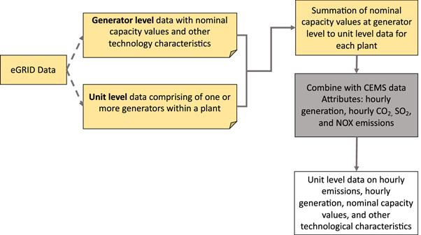
Figure 1. Schematic diagram of the process used to combine EPA's datasets: eGRID database and CEMS database. The eGRID data comprises of important technical characteristics of plant such as efficiency, prime mover type, fuel type, and name plate capacities. Since, the CEMS data is at unit level, eGRID data is first consolidated at unit level before combining with the ARP data.
Download figure:
Standard image High-resolution imageFirst, we pre-process the data within the eGRID database before combining it with the CEMS data. For this step, the attributes at generator level must be translated to the unit level within the eGRID data. The unit dataset is titled 'UNT18' and the generator dataset titled 'GEN18'. The generator dataset has the nominal capacity value of most of the turbines in the US. These capacity values are mapped to the associated units within every plant 6 , within the eGRID data. The algorithm for this mapping is developed using the Python language. In the following paragraphs, we explain in detail the steps of the algorithm for mapping generator data to unit data presented in figure 1. The heuristics for mapping differ by different types of generators and units, which we categorize into three cases. In the first case, each unit comprises a single generator (e.g., natural gas-based gas turbines). In the second case- each unit comprises more than one generator, seen for combined cycle units (combustion turbine, and bottoming cycle steam turbine). In the third case, a single generator connects to multiple units; usually, when a single steam turbine has multiple boiler units. The columns of interest from the unit's and generator's data of eGRID are unique identification number (ID) of the plants (i.e., the 'ORIS code'), state, plant name, the unique ID of the units within the plant (i.e., 'UNITID'), turbine type, primary fuel, and unique ID of the generators (i.e., 'GENID'). It is a nontrivial effort to map all the generators to their respective units, even within the eGRID database.
Case 1. One generator per unit
For the units running with single generators, both UNITID and GENID should exactly match, but the actual data requires processing before this step. Therefore, we first outer-join the GEN18 data with the UNIT18 data based on the plant's ORIS code. This ensures that each UNITID is compared with all the GENIDs within a plant, before proceeding to the mapping. We exclude the combined cycle units in this part of the algorithm, as the unit is generally a single generator, except for combined cycle units where a group of generators run together to produce electricity. Though GENIDs and UNITDs can be directly matched on a one-one basis, in approximately 30% of cases these identifiers don't exactly match. Therefore, we assign a score based on the similarity of the identifiers to each combination of UNITID and GENID using Python's SequenceMatcher from difflib library. Since each individual UNITID is compared to all GENIDs within a plant, we identify the mapping of UNITIDs with GENIDs based on the maximum resulting similarity score. For instance, a representative plant with ORIS code 7315 is shown in table 1. There is an equal number of units and generators. The unit prime mover is labeled GT (gas turbine), and the generator prime mover is correspondingly labeled GT. Each unit is an open cycle gas turbine that drives its own generator. We map the generators to the corresponding units based on the similarity in their IDs. A ratio of 1 means an exact match and ratio of 0 means no similar characters. For 9892 plants, which is about 95.4% of plants in this category, there is one-to-one mapping between units and generators. For other plants, there is no automatic way of knowing what the correct mapping would be in those cases.
Case 2. Combined Cycle units with bottoming steam fired generator- multiple generators in each unit
Table 1. A. Sample UNIT sheet in the eGRID database for the representative plant with ORIS ID 7315. The data shows that there are four units for the Almond Power Plant in California running Gas Turbines. B. A sample GEN sheet in the eGRID database for the representative plant with ORIS ID 7315. The data shows that there are in total four generators in the Almond Power Plant in California. C. Metadata for combining data from eGRID database with data from CEMS database using Plant ORISPL code and UNITID as the unique identification keys.
| A. Unit level eGRID data | |||||||
| Plant Name | ORISL plant/facility code | UNIT ID | Prime Mover | Unit bottom firing type | |||
| Almond Power Plant | 7315 | 4 | GT | CT | |||
| Almond Power Plant | 7315 | 2 | GT | CT | |||
| Almond Power Plant | 7315 | 3 | GT | CT | |||
| Almond Power Plant | 7315 | 1 | GT | CT | |||
| B. Generator level eGRID data | |||||||
| Plant Name | ORISL plant/ facility code | Generators ID | No of associated boilers | Generator Prime Mover Type | Generator nameplate capacity (MW) | ||
| Almond Power Plant | 7315 | 1 | 0 | GT | 49.5 | ||
| Almond Power Plant | 7315 | 2 | 0 | GT | 58 | ||
| Almond Power Plant | 7315 | 3 | 0 | GT | 58 | ||
| Almond Power Plant | 7315 | 4 | 0 | GT | 58 | ||
| C. Metafile combining unit level and generator level eGRID data | |||||||
| ORISL plant/facility code | UNIT ID | Generators ID | Main Power Factor | Steam bottom factor | No. of boiler | Prime mover type | Nameplate capacity (MW) |
| 7315 | 1 | 1 | 1 | 0 | 0 | GT | 49.5 |
| 7315 | 2 | 2 | 1 | 0 | 0 | GT | 58 |
| 7315 | 3 | 3 | 1 | 0 | 0 | GT | 58 |
| 7315 | 4 | 4 | 1 | 0 | 0 | GT | 58 |
For combined cycle units, there is more than one generator associated with each unit. This happens in instances where there is a bottoming cycle in a two-to-one combined cycle facility as depicted in figure 2. In that case, we assume that an equal ratio of the nominal capacity of the bottoming steam turbine generator is divided equally between each associated gas turbine generator to form a unit. Other cases could exist in which two or more combustors/boilers feed one or more steam turbines—a traditional layout for coal-fired units. In these cases, the proper fraction of electricity from each of the component generators is assigned to the appropriate unit. This case is illustrated for a representative plant with ORIS code 5567 in table 2. This plant, taken from eGRID unit and generator data, illustrates a case with two units and three generators. Furthermore, the 'unit bottom firing type' in the UNT18 sheet of eGRID shows that the unit is a combined cycle unit. The generator prime mover column reports that the 'G1' and 'G2' generators of this plant are combined cycle gas turbines, denoted by CT. Generator 'G3' is denoted as CA, indicating a combined cycle steam turbine. Furthermore the 'G3' generator has two associated boilers which matches the number of gas turbines. The resultant nominal capacity of the unit is shown in table 2. The nominal capacities of units 'CT01' and 'CT02' of ORIS code 5567 is 326 MW. This value is a summation of the nominal capacity of each CT and half of the CA generator.

Figure 2. Assumption that in any combined cycle unit, the nominal capacities of steam turbines from the eGRID database will be equally distributed and added to the nominal capacities of the combustion turbines to estimate the total capacity of the combined cycle unit in the CEMS database.
Download figure:
Standard image High-resolution imageTable 2. D. A sample UNIT sheet in the eGRID database for the representative plant with ORIS ID 55667. The data shows that there are two units for the Lower Mount Bethel Energy in Pennsylvania running Combustion Turbines with unit bottom and firing type as combined cycle. E. A sample GEN sheet in the eGRID database for the representative plant with ORIS ID 55667. The data shows that there are in total three generators in the Lower Mount Bethel Energy in Pennsylvania. F. Metadata for combining data from the eGRID database with data from the CEMS database using Plant ORISPL code and UNITID as the unique identification keys.
| D. Unit level eGRID data | ||||||||
| Plant Name | ORISL plant/facility code | UNIT ID | Prime Mover | Unit bottom firing type | ||||
| Lower Mount Bethel Energy | 55667 | CT02 | CT | CC | ||||
| Lower Mount Bethel Energy | 55667 | CT01 | CT | CC | ||||
| E. Generator level eGRID data | ||||||||
| Plant Name | ORISL plant/facility code | Generators ID | No of associated boilers | Generator Prime Mover Type | Generator nameplate capacity (MW) | |||
| Lower Mount Bethel Energy | 55667 | G1 | 0 | CT | 211.5 | |||
| Lower Mount Bethel Energy | 55667 | G2 | 0 | CT | 211.5 | |||
| Lower Mount Bethel Energy | 55667 | G3 | 2 | CA | 228.6 | |||
| F. Metafile combining unit level and generator level eGRID data | ||||||||
| ORISL plant/facility code | UNIT ID | Generators ID | Bottoming Generator ID | Main Power Factor | Steam bottom factor | No. of boiler | Prime mover type | Nameplate capacity (MW) |
| 55667 | CT01 | G1 | G3 | 1 | 0.5 | 1 | CC | 325.8 |
| 55667 | CT02 | G2 | G3 | 1 | 0.5 | 1 | CC | 325.8 |
In order to map combined cycle generators with combined cycle units, we first must map the steam turbines used in the bottoming cycle to the corresponding combustion turbines within the GEN18 sheet. These together form a unit. For this, we separate the combustion turbines and steam turbines in the generator's data of the eGRID database. The mapping of steam turbines to the combustion turbines involves two major steps. First, we check if the total number of boilers within each plant is equal to the number of combustion turbines. This is part of the quality check, where ∼2% of cases have inconsistencies in the total number of boilers reported under each plant, and a different actual number of combustion turbines using the boilers. After eliminating these cases, we calculate the similarity scores as discussed above, mapping the steam turbines to the corresponding combustion turbines. In the final step, we calculate a new total capacity at the unit level, which will divide out the nameplate capacity of the steam generators into their corresponding combustion turbines. We then repeat the process of mapping the combustion turbines of the GENIDs with the new capacities calculated at unit level to the UNITIDs within the eGRID data using the similarity scores as described previously. This creates a complete mapping of generators to units within the eGRID data for both combined cycle units, and other units.
The unit data from eGRID, including the nominal capacity values, is now combined with the CEMS data by ORIS code and UNITID. For instances where nominal capacity is missing from the CEMS data after this matching algorithm, we estimate nominal capacity levels with the maximum generation of the unit within a given year. The total number of missing values are 5% of the total number of units across all the states.
Case 3. Multiple boiler units connected to a single generator
In this case, the total number of units within a plant is greater than the number of generators. This is mostly the case for multiple boilers- designated as units connected to a large steam turbine for electricity production. Assigning based on heuristics would not guarantee a good mapping as there could be cases with a faulty IDs. Therefore, we filter out 357 plants which have more units than generators because we don't know what a good mapping would be in those cases, without manual intervention. However, we consider the annual maximum generation from the ARP data for each unit, which is a better representation of the distribution of generator load between the boilers. Overall, these cases constitute 1% of the total thermal power plants' capacity in US.
2.2. Description of key metrics used in the case studies
Loading fraction ('LF') in this study is the CEMS-reported level of generation load output divided by the nominal capacity obtained from eGRID (equation (1)). Following the matching described in section 2.1, it is now possible to estimate the LF values at both the individual unit level and the aggregate technology level (e.g., by prime mover type). Additionally, the annual capacity factor ('CF') is the total annual generation over the maximum generation (equation (2)). We compute total annual generation as the summation of the hourly generation from the CEMS data; hourly generation ('MWh') is the electricity produced (GLOAD) times the fraction of time in any given hour (equation (3)). It is not necessary that the generators always produce electricity throughout the hour, and thus the output is adjusted to an hour based on the fraction of time they operated within an hour.


where,

Where, Subscript u—Unit level
Subscript h- temporal scale, over a given hour, or over a given year
P- nominal capacity (MW)
LF- Loading fraction
CF- Annual capacity factor
α - Fraction of hour the unit is on
Load—Electricity generation (MWh)
MWh—Output in any given hour (MWh)
For analyzing the operational behavior of power plants, individual units are grouped into the broader plant level generator types. These include (i) combined cycle, (ii) open cycle gas turbines, (iii) steam turbines, and (iv) other types. In California, the analysis below is performed for combined cycle and open cycle gas turbines. Depending upon the loading fractions, the operational behavior of the units at the plant level are semi-heuristically characterized into four different buckets: start/stop, part load, near full load, and full load (table 3). The start/stop loading fractions are any generators that operate less than the minimum loading requirements [33, 34].
Table 3. Unit loading characterizations. Based on the loading fraction a unit operates at any given hour, they are categorized under start/stop, partial load, near full load, or full load. The criteria for categorizing the unit's operation is described in the table.
| Start/Stop | Partial load | Near full load | Full load | |
|---|---|---|---|---|
| Combined cycle (CC) | LF ≤ 20% | 20% < LF ≤ 75% | 75% < LF ≤ 90% | LF > 90% |
| Gas turbine (GT) | LF ≤ 40% | 40% < LF ≤ 75% | 75% < LF ≤ 90% | LF > 90% |
The efficiencies are calculated after classifying the units by generation technology at a technology level such as combined cycle unit type in California (equation (4)).

Where, Subscript t- technology type
Subscript h—temporal scale, over a given hour, or over a given year
 - Efficiency
H—Heat Input (MMBtu)
MWh—Output in any given hour (MWh)
For all temporal aggregation levels, the total energy output and heat input are calculated first, and then the efficiency, as shown in equation (4).
The average emission intensity for each LF bucket is calculated by dividing total emissions by total electricity produced for combined cycle units and open cycle gas turbine units (equation (5)).

Where, Subscript LF- Loading Fraction Category
Subscript h—temporal scale, over a given hour
I—Emissions Intensity (Tons/MWh)
EM—CO2 emissions in Tons
MWh- Electricity produced by the unit (MWh)
3. Results
In this section, we demonstrate the significance of cross referencing eGRID data with CEMS data by illustrating the changes in generation behavior by prime mover type over time and the change in operational behavior of individual turbine units within a single plant. The results section is organized as follows: we first show a break-down of changes in loading behavior of the generating plants over time for combined cycle and gas turbines, then we compare the efficiency changes between similar individual combined cycle plants during start and stop operations.
3.1. Data quality issues
Overall the eGRID dataset comprises of 10, 964 plants with 26, 709 units, and 27, 935 generators. Data quality issues arise in two cases: one from mapping generators to the units in the eGRID dataset, second while combining the resultant dataset with the CEMS data. A summary of total number of mappings considered for each case described in section 2.1 is provided in figure 3. Overall, 7% of the plants could not be mapped owing to data quality issues within the eGRID dataset between units and generators. The name plate capacity of the all the plants falling under case 3 could not be evaluated, and they were 1% of the total capacity of the plants.
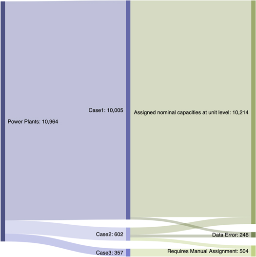
Figure 3. Summary of data points assigned with nominal capacity values at unit level in the eGRID dataset using generator level data from the same eGRID dataset. Case1: One generator per unit, Case2: Combined Cycle units with bottoming steam fired generator- multiple generators in each unit, and Case3: Multiple boiler units connected to a single generator. Note that this figure does not include the cases mapped to the ARP data.
Download figure:
Standard image High-resolution imageAround 65% of the units from the eGRID at unit level could be mapped with the UNITIDs of the ARP data. For rest of the cases, the nameplate capacities were either unavailable or the maximum value of annual generation from the ARP data was greater than the estimated nameplate capacities. In those cases, the ARP's maximum generation was considered. Apart from nameplate capacities, the combined data could indicate the unit turbine type, primary fuel, and other eGRID plant level attributes for 95% of the cases, that could be useful for the hourly level generation analysis. From the combined data, we found that for ∼80% of the observations, both estimated capacity from eGRID and maximum generation from ARP data were within 25% of each other. Overall, in this article, we hope to highlight the data quality issues, the possible range of applications with cleaner transferable data, and heuristics to be able to combine the data. If government agencies can resolve these issues, time and resources could be utilized towards meaningful applications of the data.
3.2. Change in plant loading fraction by hour of day
A combination of the CEMS data and the eGRID data allows us to estimate loading fractions in each operating hour at both individual unit level and aggregated generation technology type level.
Figure 4 shows the breakdown of the loading fractions of combined cycle units for 2011 and 2017 by the hour of the day and the resultant emissions. Results show that between the years 2011 and 2017, the total generation for starts/stops by the combined cycle units went down by 8.5%, part load went up by 15%, and full load by 10%. The change in emissions follows a similar direction of total generation. Also, the emission intensity (Ton/MWh) is largely unaffected for all the load fractions except for starts/stop between 2011 and 2017. A decrease in 8.5% in start/stops results in a decrease in 47% emissions and a decrease in 43% emissions intensity from start/stops (figure 4). The change in energy generation and emissions during start/stops and part load is concentrated during the afternoon hours, but the change in full load generation is mostly concentrated during the evening and early morning hours. Taken together, these observations illustrate a shift in CC units ramping midday in preparation for the subsequent ramp down of solar generation. This trend is further supported by changes in loading fractions at full load increasing in the late evening hours; observed LFs in this range increase by an average of 40% between 4 PM and10 PM, and by an average of 115% between 11 PM and 6 AM, concurrent with a decreasing frequency of start/stops. The decrease in emissions intensity during starts/stops could possibly attributed to several potential hypotheses such as the installation of newer power plants designed for flexible operation, a switch from more cold starts to hot starts due to better operations planning or simply the definition used to separate start/stops from part load operations. Through this article, we hope to highlight the applications of such comprehensive data, and further analysis of individual trends in detail is out of scope for this study.
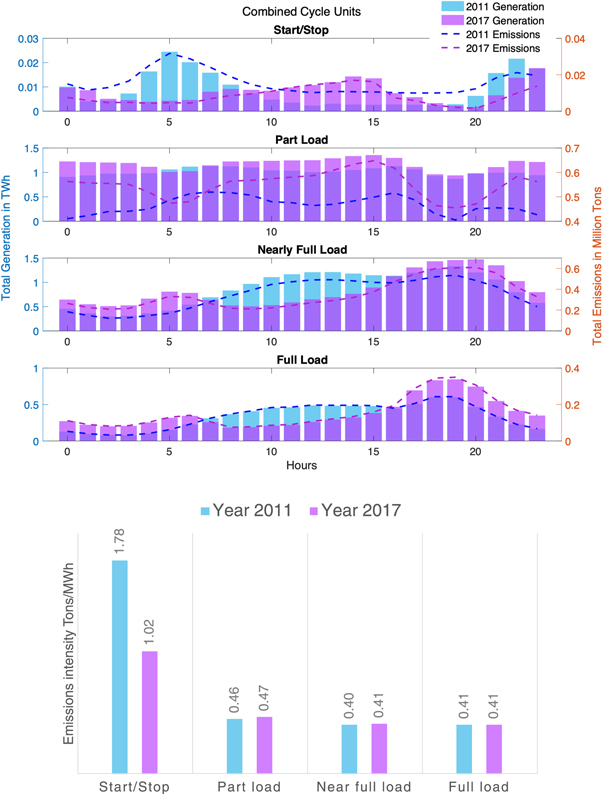
Figure 4. Topmost figure shows a breakdown of energy generation of all the combined cycle units in California from the ARP CEMS data, based on their loading fraction over a day in a year. The x-axis shows the hours in a day, the primary y-axis shows the total energy generation in TWh, and the secondary y-axis shows the total emissions in Million Tons. Each subplot indicates the grouping of the loading fraction they are operating at. The colors indicate the years considered for comparison—2011 and 2017. Bottommost figure shows the emissions intensity in Tons/MWh of the combined cycle units at different loading fractions in the x-axis. The colors indicate the years.
Download figure:
Standard image High-resolution imageFigure 5 shows the breakdown of the change in loading fractions of the open cycle gas turbine plants over 24 h in a day. Metrics displayed in figure 5 demonstrate that between 2011 and 2017, the energy output by gas turbines mostly increased at all load fractions by 2 TWh (74%). The total generation spent on starts/stops increased by 97% and was spread over the day. Also, the delivery of part-load capacities increased by 120%. The delivery of full-load capacities is largely during the evening between 4 PM and 9 PM, and it increased by 384 GWh (40%). The annual capacity factors of the gas turbines remain almost constant at 55% during 2011 and 2017. The emissions follow a similar trend to total generation. Also. The change in emissions intensity for different loading fractions is about 8%, unlike combined cycle units. What is changing is the intra-day dynamics of the GT units, primarily working towards providing flexibility when renewables are absent. Overall from these results, the gas turbine plants increased their start/stop times and their part-load generation, but decreased their peak load generation in the hours before 3 PM in the afternoon.
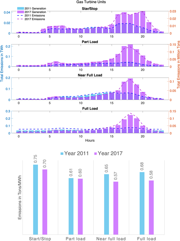
Figure 5. Topmost figure shows a breakdown of energy generation of all the open cycle gas units in California from the ARP CEMS data, based on their loading fraction over a day in a year. The x-axis shows the hours in a day, the primary y-axis shows the total energy generation in TWh, and the secondary y-axis shows the total emissions in Million Tons. Each subplot indicates the grouping of the loading fraction they are operating at. The colors indicate the years considered for comparison—2011 and 2017. Bottommost figure shows the emissions intensity in Tons/MWh of the open cycle gas units at different loading fractions in the x-axis. The colors indicate the years.
Download figure:
Standard image High-resolution imageGiven the availability of annual data from CEMS, a comprehensive analysis of intra-day operation trends can be compared over time. We present an illustration of this loading fraction analysis for combined cycle units and gas turbines in figure 6. From the figure, it can be inferred that combined cycle plants increased the generation at part load and full load from about 4:00 PM in the evening, and 50% of these units then ramp to near-full load from 5:00 PM until around 8:00 PM. The trend in start/stops shifted from morning hours before 10:00 AM to afternoon hours after 10:00 AM. For the gas turbines, the trend in generation is a more pronounced peak during the evening hours from 5 PM—7 PM, where 60% of gas turbines are operating at near to full load capacities, 33% at partial load, and 7% in starts/stops. This figure clearly demonstrates the changing operation behaviors of combined cycle plants and highlights the importance of accounting for relative loading levels in any assessment of plant operating trends.
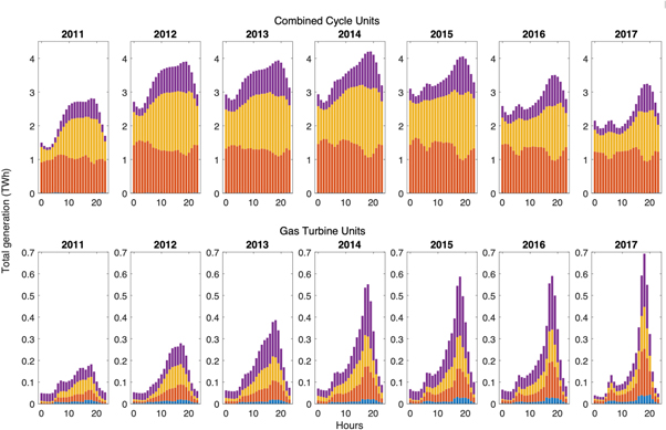
Figure 6. The breakdown of energy generation of all the combined cycle and open cycle gas turbine units in California, based on their loading fraction over a day in a year from 2011–2017. Each color indicates the range of the loading fractions. The x-axis shows the hours in a day and the y-axis shows the energy generation in TWh.
Download figure:
Standard image High-resolution image3.3. Detailed unit-level analysis of sample combined cycle plants
Figure 7 shows the efficiency and CO2 emissions rate for two different CC units (ARP ORISPL number 260, and 358). The data shows the efficiency changes and the resultant CO2 emissions of the actual units within each CC plant at different loading fractions. While these curves can be constructed using fundamental mechanical principles, the thickness of the cluster at different loading fractions could visually indicate the operational behavior of the CC units. Here, we examine both unit efficiency levels and emissions intensities. Each point on the scatter plot is the actual efficiency/CO2 emissions observed from the data set during the year 2017. The two plants considered in figure 7 have similar CC unit configurations: each plant is comprised of four combustion units and two steam turbines, with nominal capacities 1, 300 MW and 1, 100 MW, respectively. CC units in the plant with ORIS code 260 have a larger cluster of start/stops with loading fractions <20% and thus higher emissions than ORIS code 358. Furthermore, it can be inferred that because of the larger cluster of start/stops, plant 260 operates more often in part loads at loading fractions 50%–75% of the nominal capacities than the plant with ORISPL code 358.

Figure 7. Two examples of combined cycle units showing fuel efficiency, and CO2 emissions Versus loading fractions in the year 2017. The topmost figures show the efficiency versus loading fraction, and the bottom most figures show the CO2 emissions (tons/MWh) versus loading fraction. Various colors visually indicate the % of loading fraction they are operating at.
Download figure:
Standard image High-resolution image
Thus, knowledge of the nominal capacities allows us to analyze changes in the operational behavior of power plant operators at both the unit level and fleet level, which are influenced by various parameters such as the level of variable renewable generation and seasonal fluctuations. Also, this allows us to examine individual unit-level behaviors to understand the relative changes in fleet operating characteristics within a state, or across different regions.
4. Discussion
Energy models support decision making, inform policy, and grapple with issues of uncertainty and forward-looking strategies for emissions reductions. A vast amount of data describing electricity grid characteristics both at the granular plant level and the fleet level is publicly available in the US. Combining comprehensive datasets such as CEMS and eGRID provides a foundation for generating invaluable insights about changes in grid operational behavior over time, and a basis for developing metrics to aid in retrospective analysis of policy changes. The results from this study can be used to expand our understanding of the interaction between the operational behavior of generating units and the variability of renewable generation. These trends are also likely influenced by seasonal and weather patterns. We leave these inquiries to future work.
5. Conclusion
In this paper, we presented a novel approach of combining two prominent power system databases, CEMS and eGRID. We then detailed a selected set of insights from cross referencing these datasets. We assessed key generator metrics at both the fleet and individual plant level in an effort to demonstrate the application of the resultant data to inform changes in trends and operational behaviors of thermal units. Overall, we observed combined cycle plants in California between 2011 and 2017 increase their part load generation at 20%–75% nominal capacities during the morning hours and peak load generation during the evening hours. On the other hand, the gas turbines in 2017 increased both their start/stops and part load generation at 20%–75% nominal capacities. Meanwhile, they decreased their generation at full load during the afternoon hours and increased during the evening hours. Also, the increase in generation is much steeper during the recent years than the gradual change observed in 2011, from morning to evening hours. Furthermore, for combined cycle units at the plant level, we analyzed two different cases where the cluster of start/stop emissions of plant with ORISPL code 260 was a larger cluster of points compared to the plant with ORISPL code 358. Also, plant with ORISPL code 260 consistently operated at lower loading fractions at about 70% nominal capacities, alluding to larger start/stops and emissions. Further analysis can be done to identify location-based drivers and time-of-day-based drivers for these two similar plants that exhibit different operational behaviors.
These results, and the overall dataset, can be used for an array of power system analyses. This includes efforts to analyze: historical operational behavior for different grid mixes, response to renewable integration, response to policy changes, and other market-based influences. This study's data are an essential component of an integrated life cycle and cost assessment tool called SESAME. The analytical framework of SESAME encompasses the vast majority of the energy sector. Therefore, the tool can be used to conduct: (1) conventional pathway-level life cycle analysis (LCA) to study a specific technology or to comparatively assess different carbon mitigation pathways, and (2) system-level LCAs to study energy systems besides analyzing the impact of technology adoption rates, and interaction between different energy sectors [32].
Acknowledgments
This work could not be possible without the support of Dr Francis O'Sullivan, Dr Daniel Cherney, Dr Tony Wu, Dr Bryan Mignone, Dr Dimitri Papageorgiou, Dr Michael Harper, Dr Jennifer Feeley, Dr Mike Kerby, and Dr Vijay Swarup. This research was supported by ExxonMobil Research and Engineering and MIT Energy Initiative's Low-Carbon Energy Centers.
Footnotes
- 3
Since the eGRID data report (remove one of these instances of data) already combines(?) EIA-860 and EIA-923 [30], EIA forms are not considered for the study purposes.
- 4
Throughout the article, turbines and prime movers are interchangeably used, which essentially provide the mechanical input for producing electricity.
- 5
The SESAME platform focuses on accurate estimation of the GHG footprint and lifecycle and techno-economic assessment of technology pathways.
- 6
Each plant has units with individual exhaust stack that emit waste gases/pollutants where the CEMS data is recorded. These units are a combination of generators. All the generators produce electricity by converting mechanical energy through turbines to useful energy (i.e., electricity). The type of turbine/prime mover is driven by the type of fuel used to run the turbines. Throughout the article, prime-mover are used as naming convention representing the turbine types.