
Abstract
Anomalous transport due to large coherent structures, or coherent events, is studied experimentally in a magnetized toroidal discharge plasma. The present analysis emphasizes anomalous plasma losses as well as transport of electron thermal energy density across magnetic field lines. The experiment was carried out in the Blaamann device at the University of Tromsø. The diagnostics are based on data for potential, density and electron temperature variations as detected by Langmuir probes. Most of the data analysis uses conditional sampling. The flux of thermal energy density can be broken down into several components which are analyzed separately. Experimental means for obtaining the space-time variation of the complete polarization drifts are demonstrated, and the results compared with the fluctuating  -velocities. For the present conditions these polarization drifts contribute only little to the plasma losses, but for other discharge parameters in heavier gases they can be important. Our results show that while the density, the potential and the electric field variations are dominated by large scales, the vorticity of the
  -flow as well as the ion polarization drifts are strongly intermittent.
Export citation and abstract BibTeX RIS

Original content from this work may be used under the terms of the Creative Commons Attribution 4.0 license. Any further distribution of this work must maintain attribution to the author(s) and the title of the work, journal citation and DOI.
1. Introduction
Plasma losses due to large amplitude fluctuations characterize a number of laboratory devices, and similar features can be observed in nature as well. These phenomena have been studied intensively in part because of their importance for controlled thermonuclear fusion experiments. Anomalous transport can be studied also in low temperature plasma devices with a more easy diagnostic access, as compared to the hot fusion plasmas. In the present work we present data from the toroidal Blaamann device at the Arctic University of Tromsø [1], where a discharge plasma is confined by a simple toroidal magnetic field  with a possibility for adding a small vertical magnetic field. The basic physical parameters for the experiment are summarized in appendix
  in this cross section plane. The potential well gives rise to an electric field
  which induces a nearly solid body plasma rotation at a frequency
  s−1, or a period of t0 ≈ 110 µs. We took r0 to be the plasma column radius, while R0 is the major radius in the torus. The variation of the toroidal magnetic field intensity along the major radius gives rise to electron and ion
  -drifts that polarize the plasma column. The resulting polarization electric field
  induces an
  -drift. In the absence of a potential well, the plasma will be lost rapidly due to this drift. A simple analytical model [6] (paper I) illustrated the stabilizing effect of the plasma rotation. Essentially, there are two competing velocities: a characteristic rotation velocity
  taken at r = r0 and the magnetic gradient drift velocity
  in terms of a (constant) thermal particle energy
  , where uthe
is the electron thermal velocity. The x-axis is here taken along the major radius direction. Magnetic curvature drifts will contribute with a similar term to the drift velocity [7]. With the assumption
, where uthe
is the electron thermal velocity. The x-axis is here taken along the major radius direction. Magnetic curvature drifts will contribute with a similar term to the drift velocity [7]. With the assumption  the ion contribution to the large scale plasma polarization can be ignored. A significant reduction in plasma losses can be found when
  , in agreement with experimental observations. In the Blaamann plasma we have typically
  , where
  ms−1.
ms−1.
Results from the Blaamann experiment have been presented before in [8–11]. The most important new element in the present work is a comparison between the anomalous transport of plasma density and plasma thermal energy density. It was argued in paper I that the space-time variations of these two transport phenomena can be expected to be significantly different. The results presented in the following refer to one particular device, but they are relevant also for other similar experiments [2–5].
The transport of plasma is accounted for by the flux density  in terms of a quasi neutral plasma density n + n0 and a velocity
  which is unspecified for the moment. Time averaged quantities are here given by the subscript 0. These vary with position only, while the non-subscribed quantities fluctuate both with space and time. We have
  , while
  with the overline denoting time averaging. The first two terms in
  vanish by averaging, i.e.
  , and are therefore of minor interest in the following. With a continuous plasma production by the hot filament discharge, the corresponding plasma loss,
  , is non-zero. This loss can appear due to the term
  even when
  is negligible or vanishes [1, 12]. The space-time variation of the product
  has therefore received particular attention in the past [13–15].
The thermal energy density, which is also studied in the present work, is given as  , where the electron temperature is
  , assuming the ions to be cold. The flux of this quantity is
  . Here the part that vanishes by time averaging is
  , while
  . Particular attention will be given to the space time evolution of the term
  .
.
2. Estimates of plasma velocities
The plasma velocities used in the Introduction are not yet specified. Identifying  with
with  and
and  being the DC-values of the electric and magnetic fields,
  can in principle be determined by measuring the DC-potential
  . By inspection of the experimental results it is found that the DC-potential is dominated by a deep, nearly parabolic well [6, 8]. This part does not contribute to plasma losses, only to a bulk rotation of the plasma. Local deviations from this DC or steady state rotation velocity are measurable only with a nontrivial uncertainty.
The primary plasma motion is thus a rotation of the entire plasma column in the nearly parabolic well [6], with a peak in the fluctuation spectrum given by the corresponding rotation frequency [9]. A simple model, see paper I, indicates that while the plasma column rotates, it also drifts in the  -direction. The potential variations follow the density in the sense that their primary source is a polarization of the plasma by the vertical
  -motion of electrons and ions. The dominant direction of the potential dipole is thus vertical, with corrections originating from a small vertical magnetic field component and also ion-neutral collisions [6]. Additional small scale dynamics distort the primary motions of the plasma.
The fluctuations in ion velocity are determined by the fluctuations in the  -velocity with a correction originating from the ion polarization drift [7]. With constant magnetic fields we have from the cold ion momentum equation
and by an iteration
which relates fluctuations in ion velocity to fluctuations in electrostatic potential which is a measurable quantity. The second term in (2) is the ion polarization drift. Modern theories of drift wave turbulence based on the Hasegawa-Mima [16] and Hasegawa-Wakatani [17] equations rely on these drifts for constituting the important non-linear terms.
We have so far not distinguished fluctuating and steady state electrostatic potentials in (1)–(2). The coupled ion and electron dynamics in turn determine the fluctuating electric field for a given geometry [6]. The quasi-two dimensional ion dynamics assumed by (2) can be justified when  with ω being a characteristic frequency for the electric field fluctuations. This model is widely used [16, 18].
For a strictly toroidal geometry also the electrons follow the  -motion, now with polarization drifts being negligible because of the large electron cyclotron frequency. Due to the high electron mobility it will, however, be so that even a small vertical magnetic field, such as the Earth's field which is nearly vertical in Tromsø, can allow the electron velocity to have a nontrivial magnetic field aligned velocity component. Small 'winding errors' in the magnetic field coils will have similar effects. In the extreme limit, this magnetic field aligned motion will allow the electrons to reach local isothermal Boltzmann equilibria at temperature Te
. This limit can be tested experimentally by the relation
-motion, now with polarization drifts being negligible because of the large electron cyclotron frequency. Due to the high electron mobility it will, however, be so that even a small vertical magnetic field, such as the Earth's field which is nearly vertical in Tromsø, can allow the electron velocity to have a nontrivial magnetic field aligned velocity component. Small 'winding errors' in the magnetic field coils will have similar effects. In the extreme limit, this magnetic field aligned motion will allow the electrons to reach local isothermal Boltzmann equilibria at temperature Te
. This limit can be tested experimentally by the relation  with
with  being a reference density which may vary across magnetic flux tubes. To lowest approximation we can use the linear relation
  as an indicator for Boltzmann distributed electrons. For given electric field fluctuations the quasi neutrality of the plasma leads to 'locking' of the electron and ion motions.
3. Experimental conditions: description of the database
Details of the experimental set-up are given in paper I as well as elsewhere [9]. The measurements were carried out by a movable Langmuir probe. For the conditional data analysis, we have a fixed reference probe in addition. The position of the fixed reference probe and also the movable probe are shown in figure 1. The movable Langmuir probe has three probe tips. It can be used to detect plasma density as well as floating potential, as well as a triple probe for electron temperature measurements. Also steady state variations of density and floating potential can be detected by the movable Langmuir probe. A full dataset for one plasma parameter across the entire plasma column is obtained before proceeding to the next parameter.
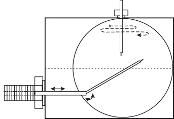
Figure 1. Schematic illustration of the positioning of the fixed (vertically placed) and movable probes in one of 4 port segments in the torus. The movable probe samples signals at 225 grid points as shown in figures 5 and 7. The main toroidal magnetic field is perpendicular to the plane of the figure. The dashed lines at the top of the figure indicates the motion of the movable probe, starting at the top, and scanning grid points horizontally, row by row.
Download figure:
Standard image High-resolution imageThe time-stationary plasma parameters  ,
,  and
and  are determined by fitting the full experimental Langmuir probe characteristics numerically at each selected position using the movable probe. This data fitting is done by an semi-automated system. Illustrative results for the spatial variations of the steady state parameters are shown in figure 2, and also elsewhere [6, 8]. We believe the resulting measurement of the steady state plasma parameters to be accurate, also concerning absolute values. Fluctuations in plasma density are on the other hand detected by the Langmuir probe current at a fixed large positive probe bias. Due to constraints in signal resolution of the acquisition system, DC values of the electron saturation current could not be obtained simultaneously with the fluctuating signal. The effective collecting area of the Langmuir probe is known to depend on the bias, so the ideal saturation of electron currents is not found. Consequently, the value of density fluctuations obtained by this method will generally be too large compared to the ideal case. Since steady state and fluctuating densities are measured by different methods, the absolute values of the two densities cannot directly be compared. As a consequence, we use different notations for fluctuations and steady state plasma densities. The relative variations found at positions distributed over the plasma cross section are on the other hand consistent.

Figure 2. Steady state, or DC, plasma parameters: density  , electron temperature
  , and plasma potential
  as measured by Langmuir probes in a cross-section of the plasma torus. The narrow central region of elevated electron temperatures indicate the location of the filament emitting the discharge electrons. The DC plasma potential has a small positive value in the white region in the upper left part of figure (c).
Download figure:
Standard image High-resolution imageFluctuations in electron temperature are detected by a triple probe. The implementation of this diagnostic method is described elsewhere [19–21]. A possible shortcoming of the method should be emphasized: it is thus known that the triple probe technique overestimates the temperature fluctuations. The main disadvantage of the triple probe method is that measurement of the plasma parameters is not performed at the same position [22]. As a result, the method cannot distinguish between a fluctuation in the parameters or its local gradient and can therefore only give an upper limit for temperature fluctuations. The temperature probe measures in principle both AC- and DC-values. In a Q-machine experiment [15] it was possible to make an independent test of the accuracy of the DC measurement, and in that case the performance was found to be satisfactory. With the limitations mentioned before, we expect the fluctuations detected by the triple probe-set also to give an adequate representation of the time varying electron temperature in our case.
Fluctuations are recorded in a position-grid of 225 points uniformly distributed inside a circle of radius 12 cm in a cross section of the plasma column. Data were acquired from the reference probe and the movable probe simultaneously, with a 2 channel digital oscilloscope (Tektronix 2430), each channel sampled at a 4 µs time resolution, with 1024 points for each data record. Ten records were obtained at each position, to give a total time series of 40.96 ms duration with 10 240 points. Finally, the fixed reference probe (see paper I) is detecting fluctuations in the floating potential each time a data-set is recorded in a grid position by the movable probe. This reference signal is the only one used for imposing conditions when applying the conditional analysis used in the present study. Time variations in floating potential are taken to be representative for time variations in plasma potential. For low frequency variations this is a good approximation for constant Te . In our case this condition is not fulfilled at the plasma edges, see figure 2, and the results are only qualitative in those regions.
4. Conditional averaging
Conditional sampling has been used as a diagnostic tool in studies of fluctuations in fluids [23] and plasmas [8, 24, 25]. The conditional average is the simplest analysis to implement in practice. It was, however, pointed out [26] that a conditional median can in reality be more relevant. The problem with this and some other similar approaches is that it requires the conditional probability density to be obtained at each position of the movable probe, which is a non-trivial extension of the data analysis. A brief summary of the method of conditional averaging and its history is given elsewhere [27]. A simple early version, the so called 'method of superposed epoch' (at times also called 'Chree analysis' after Charles Chree [28]) was in use [29] in the analysis of space data in particular. Also other methods have been proposed for identifying coherent structures embedded in random background fluctuations [30, 31]. It has been demonstrated that by proper attention to the imposed conditions, a very detailed information on the fluctuations can be obtained [10, 32–34]. If the signal follows Gaussian statistics the conditional sampling will reproduce its correlation function [27, 35]. For Gaussian random processes all available statistical information is exhausted by the space-time correlation function [36] and all other information can be deduced from it [36, 37]. Deviations of a signal from Gaussian statistics, can be measured for instance by its kurtosis K and skewness S. When S ≈ 0 and K ≈ 3 as for Gaussian probability densities, it can be necessary to have very long data series to identify possible deviations from this correlation function. Being based on one distribution function alone, the argument is, however, not complete; a joint probability density can very well represent a non-Gaussian process, even when one or both marginal distributions are Gaussian. To demonstrate deviations from Gaussian features of the signal we take also the time derivative of the original signal. Writing the standard deviation σ2 of the original signal in terms of the power spectrum G(ω) we have  . For a Gaussian process the probability density function (PDF) of the derivative process will also be a Gaussian, now with the standard deviation
  . Tests of the derivative signal can also be used to quantify deviations from Gaussian properties of a process. The conditional average will in general contain contributions also from higher order correlations [37, 38].
The probability density for the reference signal is shown in figure 3. We find here S ≈ −0.07 and K ≈ 2.92 and expect that non-Gaussian features may be manifested in the data, although we also note that significant features are likely to have their origin in higher order correlations. We obtained also the time derivative signal from the reference probe and analyzed its PDF to find a skewness S ≈ 0.01 and a kurtosis K ≈ 11.57. The derivative signal is characterized by large, randomly distributed spikes giving large excesses.
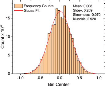
Figure 3. Probability density for the reference signal. We find here S ≈ −0.070 and K ≈ 2.922. Rather than presenting a normalized probability density, the number of counts that enter the construction of the figure are given. This shows the size of the database available for this signal. A thin red line gives the best Gaussian fit.
Download figure:
Standard image High-resolution imageThe conditional electric field is not measured directly, but it can be derived from the conditional potential as

expressed at a grid coordinate  . With the given sampling rate an estimate of the time differential of the signal can be found, and thereby also an estimate for the conditional ion polarization drift [7] in the form
  , with Ωci
being the ion cyclotron frequency. The given expression for the polarization drift is determined at each grid-position by a discrete time differentiation.
, with Ωci
being the ion cyclotron frequency. The given expression for the polarization drift is determined at each grid-position by a discrete time differentiation.
A relation like (3) is exact for time stationary processes: in an ideal experiment with a spatially dense probe array measuring potentials at all positions simultaneously, the conditional electric field could be obtained by the local potential differences in the probe plane. The result would be identical to (3).
Often the importance of the ion polarization drift is estimated by the fluctuation spectrum of the electrostatic potential or the electric field to determine the significance of the part of the spectrum that is close to the ion cyclotron frequency. In our case we find significant fluctuation amplitudes in the spectrum only at and below ∼50 kHz, i.e. ∼1/10 of the ion cyclotron frequency, see figure 4. When the spectral power at frequencies comparable to Ωci
is small, it is often argued that the ion polarization drift is negligible. The argument seems logical, but it breaks down if the time and space derivatives of the electric field are strongly intermittent. In that case the local polarization drift can be significant even if it is globally small, on average. To analyze this question in our experiment, the temporally varying conditionally averaged electric field is differentiated by a finite difference scheme applied to the time series at each spatial position. Similarly, a numerical differentiation of  , can give an estimate for
  , which for constant
  is the local conditional rotation of the
  -velocity field.
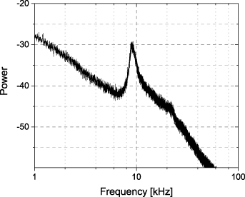
Figure 4. Power spectrum of the fluctuations in the electrostatic potential as sampled by the fixed reference probe. The spectrum is shown on double logarithmic scales. The narrow peak in the spectrum corresponds to the rotation frequency of the plasma column.
Download figure:
Standard image High-resolution imageThe instantaneous flux-values of the plasma density or the energy density are not available in our experiment. We suggest in the following an approximation that can be used to construct conditional averages of these fluxes. At a grid-position  any signal can be written as
  , where
  is the deviation from the conditional average indicated by the subscript c, so that
  and similarly for other fluctuating quantities. The component of the conditional flux density can then be written as
where the subscript x indicates the relevant electric field component, perpendicular to the flux direction at the grid-position  . If the conditional variance discussed in the following section 4.1 is small or vanishing in a region near the time and location for the imposed condition, then we have the conditional average being close to the actual variation of the fluctuating quantity in a given realization locally in space and time. If, for instance, a prominent large coherent structure (or rather a coherent event) is present in the turbulent fluctuations with only a low level of additional noise, then the conditional average will reproduce this structure with a small conditional variance [8]. In such cases
  and
and  are small and the averages of their products negligible. The averaged product in the last term in (4) can then be ignored. In this case a significant simplification is obtained in the analysis of the data in terms of conditional averages of the individual components of the products. It is then possible to present data for the conditional plasma flux in a full cross section from single probe measurements giving fluctuations in plasma density and also in potential separately. The conditional thermal energy density flux can be obtained similarly when also data for the fluctuating electron temperature are available. Consequently, also turbulent transport of the electron thermal energy density can be studied. Phase relations between density and potential are retained in the conditionally averaged quantities since the averages are connected by the conditions imposed on the reference signal. These phase relations are important for correct estimates of, e.g. the conditionally averaged
  -transport. The present approach offers a great simplification compared to the ideal measurement requiring simultaneous detection of plasma density, potential and electron temperature. Conditions for omitting the last term in (4) are discussed in the following sections.
4.1. Conditional reproducibility
To substantiate the assumption concerning the conditional reproducibility we use the definition introduced originally in [8],

expressed in terms of the conditional variance
here written for the potential fluctuation, with similar definitions for the other variables. We note that  . The definitions used here (the normalizations in particular) are slightly different from some used elsewhere [26]. Details of the normalized conditional variance is discussed elsewhere [8, 15, 26].
In general  will be varying with space and time as measured with respect to the reference position and time
  . When
  the value of the variable, the potential for instance, is the same in every realization. For those times and positions the last term in (4) is vanishing. The conditional variance and reproducibility can be determined experimentally, with results to be shown later.
5. Results
Conditionally averaged density and potential variations for various plasma conditions in the Blaamann device have been shown elsewhere [8, 9]. Here only some selected related results are presented, see the first and third entries in figure 5. The flute nature of the observed fluctuations was explicitly demonstrated in a previous related study [8].
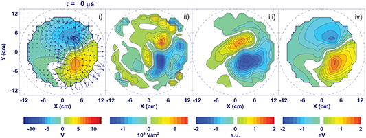
Figure 5. The figure shows conditional sampling results of i) the conditionally averaged floating potential  , ii) the estimate of the local
  derived from it, iii) the fluctuating plasma density
  detected through the electron saturation current to a Langmuir probe, and iv) the electron temperature
  across the full plasma cross section, all obtained at the reference time, τ = 0. The condition imposed on the reference signal (the floating potential at the fixed probe) was in this case
  in terms of the standard deviation σ of the reference signal. Superimposed on the conditionally averaged potential we give the directions and relative magnitudes of the local electric field vectors obtained by numerical differentiation of the potential in (i). As explained in the main text, the variation of
  is presented in arbitrary units (a.u.) since it is obtained by a different method as
  . As an order of magnitude, the unit value on the corresponding color code corresponds to 5 × 10¹⁶ m−3. Small black dots in (i) give the sampling grid positions.
Download figure:
Standard image High-resolution imageBy recording AC signals, we are in effect measuring fluctuations relative to a time average. For instance, when measuring the density in a case where the plasma column is displaced with respect to its average position, it will be found that the spatial variation of the signal appears as a dipolar structure, where a density depletion appears next to a density enhancement. In case the density variation was solely due to a rotation of the plasma column in the parabolic potential, a dipolar density structure will be found to be directed towards the plasma center at all times. This seems not to be the case, indicating a temporal evolution and deformation of the plasma column as it rotates, in agreement also with the simplified numerical study in paper I. Only in a first approximation, the deformation of the plasma column can be seen as a 'tilting'. Depending on plasma conditions as well as the condition imposed on the reference signal, the relative conditional density variation with respect to the average value  can be large at some space-time positions, even up to 25 − 50%.
Several features are noticeable in figure 5. First of all there is a significant difference between  and
and  , demonstrating that the electrons are not in a near Boltzmann equilibrium. In that case the two averages should be close, i.e. directly proportional in the linearized limit. While the potential variation and the electric field derived from it is dominated by a large scale 'global' variation, we find a strong intermittency in the vorticity
  of the conditional
  -drift. The intermittent feature remained when delaying or advancing the sampling time τ with respect to the reference time. The fine-scale structures observed in
  were found to follow the bulk plasma rotation, at least to a first approximation.
The conditionally averaged potential and electron temperature appear to be similar. The potential variation is to lowest order induced by the plasma polarization caused by the  electron drift in the vertical direction. This electron drift is, however, selective in the sense that the most energetic parts of the electron thermal population are drifting faster to collect at the position where the polarizing potential is the largest. These regions will then appear as the 'hottest' compared to the time average when the electron temperature is monitored. A lowest order similarity between the Te
and the φ variations is thus to be expected. In figure 5 a difference is noted mostly in the relative asymmetry of the positive and negative potential and temperature variations, respectively. The similarity erodes when τ is either increased or decreased with respect to the reference time τ = 0. The similarity depends to a lesser degree on the imposed condition on the reference signal.
electron drift in the vertical direction. This electron drift is, however, selective in the sense that the most energetic parts of the electron thermal population are drifting faster to collect at the position where the polarizing potential is the largest. These regions will then appear as the 'hottest' compared to the time average when the electron temperature is monitored. A lowest order similarity between the Te
and the φ variations is thus to be expected. In figure 5 a difference is noted mostly in the relative asymmetry of the positive and negative potential and temperature variations, respectively. The similarity erodes when τ is either increased or decreased with respect to the reference time τ = 0. The similarity depends to a lesser degree on the imposed condition on the reference signal.
The conditional variance and reproducibility discussed in sections 4 and 4.1 can be determined experimentally, and we show illustrative results in figure 6, all taken at the reference time τ = 0. The maximum reproducibility is found in the vicinity of the reference probe, but the value of  depends significantly on the physical variable it represents. The conditional reproducibility is thus moderate for the fluctuations in density, while it is significant for both potential and electron temperature, best for the latter quantity. All results refer to the value of the imposed condition, here
  . The arguments for ignoring the last term in (4) are thus reasonably well fulfilled, in particular as far as the fluctuations in potential and electron temperature are concerned in regions near the reference probe for conditional fluctuations sampled close to the reference time. For other space-time variables involving fluctuating densities, the results shown in figure 6 are representative or at least illustrative: even in case the last term in (4) is finite, it can still be so that the first term is dominant.
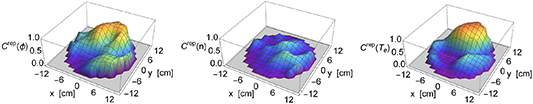
Figure 6. Spatial variation of the conditional reproducibility as defined by (5) and (6) shown here for fluctuations in density, potential and electron temperature. All figures are taken at the reference time τ = 0. The maximum values are  .
.  , and
, and  . The figures are shown as surface plots to be clearly distinguishable from the results in figure 5.
Download figure:
Standard image High-resolution imageThe present analysis emphasizes large amplitude coherent structures. We do not show results for small values of the imposed conditions. In that case it turns out that the noise becomes dominating, and the conditional reproducibility (5) becomes small. Conditional averaging as used here works only for large values (in terms of the standard deviations of the signal) of the imposed conditions, i.e. large amplitude structures. On the other hand, if the condition applied to the reference signal is too large, the condition will be met only rarely and the signal-to-noise ratio in the result becomes poor.
5.1. Transport by plasma fluctuations
Anomalous transport in the Blaamann plasma was studied by analyzing the data-set described before. The transport due to fluctuations depends in particular also on the electron dynamics, with a limiting case being Boltzmann distributed electrons, see also discussion in appendix
As discussed in paper I, a small vertical magnetic field component could in principle allow a flow of electrons from density enhancements to density depletions. If collisions were insufficient to impede this flow, an isothermal Boltzmann distribution could then be established also in our device. In that case we would have  . This relation was found to be in variance with the experimental conditions [39], see also figure 5. To test an alternative we correlated density with electric field variations [40]. This correlation was not significant and also the possibility of a local relation n ∼ E can be excluded, although it was found to have promise in other plasma conditions, in the lower parts of the ionosphere in particular. We believe that for our conditions, the most plausible general relation between plasma density and potential is non-local in space and time.
Characteristic results for the transport of plasma and thermal energy densities in the Blaamann device are presented in figure 7. Figures are shown for times  and 24 µs with respect to the reference time where the condition is imposed on the reference signal (the floating potential at the fixed probe). The magnetic field is taken to be a constant, B0(r = 0). The figure covers a time interval of 48 µs, i.e. approximately 1/2 of a plasma rotation. If the time interval is extended, the conditional averages damp out and the conditional standard deviations increase to become close to their unconditional value. In the case shown the imposed condition on the reference signal was
  in terms of the standard deviation σ of the signal. One observation is that
  and
and  are nearly in counter-phase for the relevant time-span so that the contribution to the net energy flux
  , is negative or vanishing. This latter quantity is composed of averages over three fluctuating quantities and is consequently of smaller numerical magnitude compared to the results in the third column in figure 7. As predicted by a simple model [6] we find a rotation of a dipolar density variation, while on the same time-scale a potential dipole retains a dominant vertical component during the motion of the plasma column [6]. The potential variation is induced by a polarization caused predominantly by the near vertical
  electron drift.
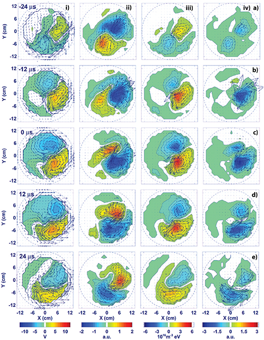
Figure 7. The reference times  µs are labeled (a), (b), etc, while the columns containing the sampled quantities are labeled (i), ii), etc Column (i) shows the variation of the velocity field
  with arrows. The results are superimposed on
  from which they are derived. Column ii) shows the corresponding time evolution of estimates for the plasma transport
  shown by arrows superimposed on the conditional density variation
  entering the estimate. Column iii) shows corresponding variations of
  with vectors at each spatial grid position superimposed on
  . Superimposed on
  , the last column iv) shows
  with vectors. For reasons discussed before, quantities containing
  are given in arbitrary units. As an estimate we can use the unit value on the color code of column ii) as corresponding to 5 × 10¹⁶ m−3, while in column iv) it will be 5 × 10¹⁶ m−3eV.
Download figure:
Standard image High-resolution image5.2. The ion polarization drifts
As most related studies, the results presented here are based on identifying the local bulk plasma flow velocity with the  -velocity. As is well known, this is merely the lowest order contribution from an expansion where the next term is the polarization drift. Usually this latter contribution is assumed to be of second order in the expansion, see (2), but as argued before, its estimate is in general not simple. The data allow a calculation of the polarization drifts by a numerical time differentiation of the electric field. It turns out that the polarization drift is small in our case, but its space-time variation is interesting nonetheless and it is illustrated here in figure 8. As seen, the strongest time variation is localized to the spatial region where the electric fields are largest (see figure 5), and the structures are following the plasma rotation. The observed time variation is therefore mostly due to a spatial structure swept past the detecting point due to the bulk plasma motion, see for instance times τ = 12 and 24 µs in figure 5. In the co-moving frame (with a velocity
  , which for our conditions is dominated by the rotation velocity UR
) we might in principle find
, which for our conditions is dominated by the rotation velocity UR
) we might in principle find  to be small. Its conditional average can be estimated by a product of conditional averages as used in the foregoing analysis. A term
  is negligible compared to
  . In figure 8 we show
  in ii) and
  in iii).

Figure 8. Illustration of the conditionally averaged polarization drift terms  in column ii) and
  in column iii) for the same times as in figure 7. The drift velocities are indicated by local arrows, superposed a color coded magnitude of the numerical value of the corresponding drift velocity. For reference, column (i) shows the space-time variations of the conditionally averaged
  -drift velocities with vectors superposed on the color coded magnitude of the corresponding velocity. The polarization drifts are small for the present discharge conditions since we have light ions, i.e. Helium. The polarization drifts are characterized by strong intermittency: the structures in column ii) are elongated having scales 6–7 cm, while in column iii) they are somewhat smaller, approaching the spatial grid resolution, but we nonetheless find a systematic motion also of these structures.
Download figure:
Standard image High-resolution image
The polarization drifts are in our case small compared to the  -velocity. The plasma discharge is for the present case in Helium. It is anticipated that use of a heavier gas like Argon with a smaller ion cyclotron frequency but the same potential well, can give rise to a more significant contribution from the ion polarization drift in Blaamann and similar devices. The plasma density gradients and corresponding diamagnetic drifts will be similar also for heavier gases (other parameters being the same) but, measured in the relevant units of the larger ion Larmor radius for a heavier gas, the gradients will appear steeper. Although the ion polarization drifts are small in the present experiment, at most 2 - 5% of the local
  -velocity, we note that they are indeed strongly spatially intermittent as found by inspection of figure 8. Even though the ion polarization drifts are small, they contribute to the plasma compression where the
  drift is incompressible for constant B0. At times and positions where
  is in the azimuthal direction, the polarization drift can be the only source (albeit small) of plasma losses.
A term  was not analyzed. The term can be expressed analytically if we take
  to be a good approximation. Then we have
see figure 5(a) for  . Also this term contributes in (1), to lowest order.
6. Discussion and conclusions
Electrostatic, low frequency fluctuations and their associated anomalous plasma transport have been studied by conditional sampling in the Blaamann device. It is known, see also the discussion in appendix  -drifts with Boltzmann distributed electrons will not give rise to any anomalous plasma transport through a closed surface following a magnetic flux-tube. It is explicitly demonstrated that the electrons are not isothermally Boltzmann distributed in our plasma. In general the transport appears to be of 'bursty' nature [2, 25], with some structures appearing as 'streamers' [11, 40, 41]. By inspection of the data it is found that there are time intervals where the transport is actually into the plasma and indeed several experiments report inwards propagating bursts [42, 43]. The bursty event can be classified as 'global' since they cover most of the plasma cross section. Such scenarios can be recognized at several instances in the data, but there are also many local events, in particular near the plasma surface at large radial positions. The consequence of these global and local structures, or coherent events, is a net transport out of the plasma resulting in losses to the walls. Synthetic data series can be constructed [40, 44] to give solvable models for statistical details in the local plasma transport.
As mentioned in section 5.2 there are times where the strongly intermittent polarization drifts, albeit small, are the only sources of plasma losses in Blaamann-like devices. These losses can have the form of small scale structures, or 'blobs' which can be modeled analytically as well [44]. It has been argued [11] that not only the magnitudes, but also the durations and frequencies of such streamers and blobs need to be considered to fully understand their contribution to the wall-loading of the confining vessels. These properties can be modeled by proper a priory given information. Indications are [45] that isolated blobs move with constant acceleration, rather than a constant velocity.
The fluctuations described in the present study are dominated by large spatial scales, rather than broad band turbulence composed by randomly phased waves. Since the fluctuations are strongly magnetic field aligned [8] and thus nearly 2 dimensional, it is a possibility that this is due to an inverse cascade [46–48], where the spectral energy condenses at the largest spatial scales of the system. This phenomenon seems to be an intrinsic feature of turbulence in 2 spatial dimensions. Attempts to give experimental evidence for an inverse cascade in 2 dimensional ('flute type') turbulence in a magnetized plasma device were, however, not conclusive [49] but the suggested methods may be useful for other studies.
Although the fluctuating properties of the plasma in Blaamann seem to be dominated by large scale structures of size close to the plasma diameter, i.e. 20 cm, it is interesting that the vorticity  shows strongly intermittent features of scales almost an order of magnitude smaller, i.e. ∼3 cm. Similarly, also the polarization drift is spatially localized on scales of the order of ∼6 cm. Some of the finest details are comparable in size to the spatial grid resolution, and therefore only illustrative. In our device the transport due to the polarization drift is a small correction (a few %) to the
  -flow, but in discharges using other and heavier gases where the ion cyclotron frequency is smaller, it can be of importance. Our results show how the relative importance of these transport mechanisms can be estimated by extended use of conditional averaging. The results summarized in the present work refer to one particular type of device (here represented by the Blaamann device), but we believe the results to have more general applicability. The intermittent features are associated with derivatives (spatial or temporal) of the conditionally averaged electrostatic potential. This potential is dominated by large scale structures as seen in figure 5. The derivations emphasize localized gradients on smaller scales in these structures.
In a linear device it was possible to make an external perturbation of the time variation of the net plasma transport across magnetic field lines [49]. It could be interesting to make a similar study in a Blaamann type device. This can be done by, for instance, inserting a small circular semi-transparent grid where the potential, and thereby the particle absorption by the grid, can be controlled in a thin magnetic flux tube, e.g. by applying a short pulse.
Acknowledgments
The data-sets used in the present analysis were obtained in the Blaamann device at the Department of Physics and Technology, the Arctic University of Tromsø. The experiment has now been dismantled on the request of the Norwegian National Science Foundation. We would like to thank colleagues, students, and the technical staff for their contributions to the work on this experiment. In particular, we thank Terje Brundtland for his enthusiasm and tireless work in the construction and maintenance of the device. The authors also acknowledge results obtained by Dr Lucia Cartegni when working with the Blaamann experiment. This work was funded by The Department of Physics and Technology, UiT.
Appendix A.: Basic experimental parameters
For completeness, some of the basic parameters of the experiment are summarized in this appendix, see table A1. A cross section with probe positioning is shown in figure 1 and spatial variation of some basic plasma parameters in figure 2. The experiment is carried out in a magnetized toroidal plasma without magnetic transform, with major and minor radii being R0 = 0.67 m and r0 = 0.135 m.
Table A1. Summary of basic plasma parameters, assuming singly charged helium ions. For estimating frequencies (plasma or cyclotron) we use parameters in the plasma center.
| Toroidal magnetic field at R0 | 0.154 T |
| Vertical magnetic field | 55 × 10−6 T |
| Neutral He-pressure | 10−3 mbar |
| Maximum plasma density, n0 | 1.6 × 10¹⁷ m−3 |
| Reference electron temperature, Te | 5 eV |
| Ion temperature, Ti | 0.05 eV |
| Electron plasma frequency, ωpe | 1.8 × 10¹⁰ s−1 |
| Ion plasma frequency, Ωpi | 2.1 × 10⁸ s−1 |
| Electron Debye length, λDe | 50 × 10−6 m |
| Sound speed, Cs | 11 × 103 m s−1 |
| Electron thermal velocity, uthe | 0.94 × 10⁶ m s−1 |
| Ion thermal velocity, uthi | 103 m s−1 |
Electron  and curvature and curvature | 60 m s−1 |
| drift velocity | |
Ion  and curvature drift velocity and curvature drift velocity | 0.6 m s−1 |
| Electron cyclotron frequency, ωce | 27 × 109 s−1 |
| Ion cyclotron frequency, Ωci | 3.7 × 10⁶ s−1 |
| Average electron Larmor radius | 35 × 10−6 m |
| Average ion Larmor radius | 0.27 × 10⁻³ m |
| Ion-electron collision frequency, νe,i | 80 × 103 s−1 |
| Electron-neutral He cross-section, σe,n | 6 × 10⁻²⁰ m2 |
| Ion-neutral He cross-section, σi,n | 65 × 10−20 m2 |
Electron-neutral mean free path, 
| 0.7 m |
Ion-neutral mean free path, 
| 64 × 10−3 m |
| Electron-He collision frequency, νe,n | 1.4 × 10⁶ s−1 |
| Ion-He collision frequency, νi,n | 16 × 103 s−1 |
Appendix B.: Transport with isothermally Boltzmann distributed electrons
In a locally homogeneously magnetized plasma column, the net  -transport out of a closed plasma surface vanishes for electrostatic fluctuations in case the electrons are Boltzmann distributed at all times. Taking a closed contour
  following an equi-density level
  we integrate the plasma flux across a surface
  with unit length along a homogeneous magnetic field
  and a cross section defined by
  . The curve
  will have a finite length for relevant conditions. The surface
  bounds a volume
  . The net plasma flux through the surface
  can be expressed as
  , with
  being a unit vector perpendicular to the given surface element. With
  constant, the integral can be rewritten as
The result remains correct for the more general local relation  , where we have
  . The relation (B1) holds at any time t, not only as a time average. The expression (B1) will be non-vanishing when
  .
.
The plasma flux contribution from the polarization drift can be discussed in the same way to give
where the first term in the parenthesis of the integrand is E2 and ∇2
φ/B is again the magnitude of the vorticity of the  -velocity field. This quantity was analyzed separately, see figure 5. In reality, only the time average of (B2) is relevant.