


Abstract
Random deposition with a relaxation model in (u, v) flower networks is studied. In a (2, 2) flower network, the surface width W(t, N) was found to grow as b ln t in the early period and follows a ln N in the saturated regime, where t and N are the evolution time and the number of nodes in the network, respectively. The dynamic exponent z, obtained by the relation z = a/b, was z ≈ 2.11(10), which is consistent with the random walk exponent dw = 2 in the network. For u + v ⩾ 5(u ⩾ 2, v ⩾ u), i.e. the (2, 3) and (3, 3) flower networks, the surface width grows following power-law behavior with some corrections, where the growth exponent β and roughness exponent α are controlled by spectral dimension ds and fractal dimension df of the substrate network.
Export citation and abstract BibTeX RIS
1. Introduction
During the last several decades, considerable efforts have been devoted to the study of the roughness of growing surfaces in various growth models and stochastic Langevin equations [1–4]. Surface roughening phenomena are associated with a wide range of systems, such as domain walls in the random bond Ising model [5], ballistic aggregation [6], epitaxial film growth ([7] and references therein), and directed polymers in a random potential [8]. Growth phenomena are characterized by the critical exponents that describe the dynamics of the surface width. The surface width in a system of size L is defined by the standard deviation of the heights, given as

where h(x, t) is the local height variable of the surface,  is its spatial average at time t, and ⟨...⟩ denotes the average over many samples. For finite-size systems, the mean square surface width satisfies the Family–Vicsek scaling function [9]

where the extreme values of the scaling function are given as f(u) → u2β for u ≪ 1 and f(u) → const. for u ≫ 1, and β and α are the growth and roughness exponents, respectively. The dynamic exponent z is given by the relation z = α/β.
Various growth models have been classified to a few distinct universality classes, each corresponding to a particular continuum equation for a coarse-grained height variable h(x, t). One of the simple growth models is random deposition with surface relaxation, also known as the Family model [10], in which a particle is deposited on a randomly selected site and subsequently allowed to diffuse to the nearest-neighbor site that has the lowest height.
It has been claimed that the surface width of the Family model can be described by the Edwards–Wilkinson (EW) equation [11], given by

where η is the uncorrelated random noise satisfying

the parameter D describing the strength of noise and d being the substrate dimension. The linear EW equation can be solved exactly in a regular substrate and the critical exponents are obtained as α = (2 − d)/2, β = (2 − d)/4 and z = 2.
On a regular lattice, the surface width grown by the Family model was indeed consistent with that of the EW equation. In d = 2, the surface width grows logarithmically with t at the beginning and becomes saturated at ln L. Above the critical dimension dc = 2, the surface becomes flat. On a scale-free (non-fractal small world) network [12–14], on the other hand, the saturated width Ws grown by the relaxation model was found to depend on the degree exponent γ [15], i.e.

where Ws(∞) ≡ Ws(N → ∞) and Δ = (γ − 2)(γ − 1). In the scale-free complex network, the degree distribution follows the power law P(k) ∼ k−γ . The diffusion term of the EW equation in complex networks is interpreted as ∇2 hi = ∑j (hj − hi ), where j is the nearest-neighbor connected sites of i. The logarithmic scaling behavior for γ < 3 was not represented by the direct integration of the EW equation and, therefore, the random deposition with surface relaxation model does not belong to the EW class in scale-free networks [15].
In this paper, we consider the surface growth by the Family model in different types of scale-free networks, i.e. in (u, v) flower networks [16, 17]. These (u, v) flower networks are fractal networks and also scale-free networks. On regular fractal substrates, such as Sierpinski gaskets and checkerboard fractals, the growth and roughness exponents were represented by the spectral and fractal dimensions of the substrate [18–21]. The dynamic exponent was consistent with the fractal dimension of random walks on the substrate, dw, defined by the mean square end-to-end distance  . The degree distribution becomes P(k) = δ(k − 4) in both the square lattice and Sierpinski gasket. However P(k) has a power behavior P(k) ∼ k−γ
for scale-free networks and has a very heavy tail with a non-negligible amount of nodes of a very large degree. It would be interesting to examine whether or not the heterogeneity in the degree distribution can change the scaling of the surface width.
. The degree distribution becomes P(k) = δ(k − 4) in both the square lattice and Sierpinski gasket. However P(k) has a power behavior P(k) ∼ k−γ
for scale-free networks and has a very heavy tail with a non-negligible amount of nodes of a very large degree. It would be interesting to examine whether or not the heterogeneity in the degree distribution can change the scaling of the surface width.
In section 2, the generation of the (u, v) flower networks and the relaxation model are described. In section 3, the results of the Monte Carlo simulations for the (u, v) flower networks are presented, together with the relevant discussions. In section 4, the summary and conclusions are presented.
2. The ( , v) flower and the relaxation model

The (u, v) flower networks are generated following [22]. The 0th generation network consists of two nodes and one link between them. For a given nth generation, the (n + 1)th generation is obtained recursively by replacing the link with two parallel paths: one has (u − 1) nodes and u links, the other has (v − 1) nodes and v links (v ⩾ u), as shown in figure 1 for u = v = 2 up to n = 3.
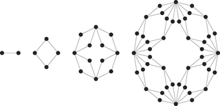
Figure 1. Generation of the (2, 2) flower network for n = 0, 1, 2, and 3.
Download figure:
Standard image High-resolution imageThe number of links of (u, v) flower at the nth generation is

where w = u + v. The number of nodes obeys the recursion relation Nn = wNn−1 − w with N1 = w, which yields

The resulting (u, v) flower networks are known to be a scale-free network with the degree exponent γ given by [16, 22]

The size of the nth generation of the (u, v) flower networks is represented by a diameter Ln , defined by the longest length among the shortest path between any two nodes. For u = 1, the diameter Ln scales with n, whereas, for u > 1, it grows as a power of n, i.e.

(we consider in this paper only the cases u > 1). Using Nn ∼ (u + v)n (equation (7)), the diameter of the network is obtained as

for a large n limit. The fractal dimension df and the spectral dimension ds were also obtained as

Using the Alexander–Orbach scaling relation [23], the random-walk fractal dimension is given as dw = ln(u v)/ln u.
The relaxation model (Family model) is simple, as described briefly in section 1. From the flat substrate, a particle is deposited on a randomly selected site and subsequently diffuses one step to the nearest-neighbor site with the lowest height. If the height of the current site is lower than any of the neighboring sites, the particle stays on the current site. If two or more neighboring sites are of the same height and lower, the particle diffuses randomly to one of those sites. The time t is defined as the number of Monte Carlo steps.
The growth exponent β of the relaxation model in the fractal substrate can be derived from a simple mapping of the model to the random deposition model. For a random deposition, the surface width grows in time as W2(t) ∼ t. For the relaxation model, the surface growth is assumed to be similar to that of the random deposition with correlations, and the correlation length increases in time as the rms end-to-end distance of random walks, i.e.  . The number of accessible sites S(t) of the random walker at the time t is
  , where df is the fractal dimension of the substrate. Since the number of accessible sites S(t) is described by the spectral dimension ds

the scaling relation ds = 2df/dw, known as the Alexander–Orbach scaling relation, holds [23]. The surface width of random deposition within a correlation length ξ thus follows  , so,
, so,  , where P(t) is the probability of random walks to return to origin and is associated with the spectral dimension via
  . The growth exponent β on the fractal substrate is thus obtained from W2(t) ∼ t2β
. The dynamic exponent of the relation model can be assumed to be the same as the fractal dimension of random walks on the fractal substrate, i.e. z = dw. With this and the scaling relation α = zβ, the roughness exponent is estimated as
. The growth exponent β on the fractal substrate is thus obtained from W2(t) ∼ t2β
. The dynamic exponent of the relation model can be assumed to be the same as the fractal dimension of random walks on the fractal substrate, i.e. z = dw. With this and the scaling relation α = zβ, the roughness exponent is estimated as

The results of equation (13) were also obtained by the author and his colleague by power counting the fractional EW equation [21]. For ds < 2, it is expected that both β and α are positive. For ds = 2, on the other hand, both exponents are expected to be zero, and the width grows at most logarithmically in time. It would thus be interesting to examine whether the exponents of the relaxation model in various (u, v) flower networks follow the expectations.
3. Numerical results
Simulations of the relaxation model were performed in various (u, v) flower networks. The surface widths were measured by direct Monte Carlo simulations, and the growth and roughness exponents were measured coupled with scaling analysis of the surface width.
3.1. Results from a (2, 2) flower network
We carried out simulations for the relaxation model in a (2, 2) flower network. This (2, 2) flower network is a scale-free, but not small world, network with γ = 3, df = 2, and ds = 2 [16]. The size of system is assumed to be the diameter Ln
= 2n
for u = v = 2 and  (equation (10)) in a large n limit.
Figure 2 shows the numerical data plotted on a semi-logarithmic scale; (a) is the surface width W(Ln , t) against the growth time t for various values of Ln and (b) is the saturated width Ws(Ln ) against the diameter Ln , both on a semi-logarithmic scale. The plots in the figure show that W(Ln , t) grows as ln t in the early period and becomes saturated at Ws(L), which also grows logarithmically as L, i.e.

The best fit of the numerical data yielded a = 0.442(9) and b = 0.210(10). Now, assuming the scaling form of the surface width,

where the scaling function g(x) is given as g(x) ∼ xb
for x ≪ 1 and g(x) = const. for x ≫ 1, the dynamic exponent z is given as  . Figure 3 shows the scaling plot of the data using the values of b, a and z; data scales fairly well. Because
  in the (2, 2) flower network,
  . Ws(N) grows logarithmically with N even for γ = 3. This logarithmic dependence is consistent with an earlier work [15] on scale-free complex networks for γ < 3. Therefore, the surface growth in a (2, 2) flower network is represented by the critical exponents β = α = 0 and z = 2.1(1). It should be noted that the exponents β and α are precisely the value predicted by equation (13). We obtain dw = 2df/ds = 2 from the Alexander–Orbach relation [23]. Therefore, the present estimate of z = 2.1(1) is assumed to be consistent with the fractal dimension of random walks dw = 2 within an error bound. It is, thus, surmised that the relation z = dw is generally true for the relaxation model in (u, v) flower networks.

Figure 2. The surface width generated using the relaxation model in (2, 2) flower network of various generations n. (a) Is the root mean square surface width W(Ln , t) against evolution time t and (b) is the saturate width Ws(Ln ) against the diameter of the network. In (a), the solid lines are the Monte Carlo data for various n values and the dashed line is the fitting line of W(L, t) = 0.210 ln t + 0.46; in (b) the solid line is for 0.442 ln Ln .
Download figure:
Standard image High-resolution image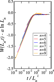
Figure 3. The scaling plot of surface width using the estimated values of a = 0.442 and z = 2.11 in (2, 2) flower network.
Download figure:
Standard image High-resolution image3.2. Results from (2, 3) and (3, 3) u v networks
Simulations of the relaxation model in other u v flower networks for (u, v) = (2, 3) and (3, 3) were also carried out. For the (2, 3) flower network, γ ≃ 3.32, df ≃ 2.32, and ds ≃ 1.80, and for the (3, 3) flower network, γ ≃ 3.58 and df ≃ ds ≃ 1.631. Because ds < 2, equation (13) predicts β > 0 on these fractal scale-free networks. We present the full simulation data of the relaxation model in a (3, 3) flower network.
Figure 4 shows the mean square surface width in a (3, 3) flower network as a function of evolution time on a double logarithmic scale. It is clear from the plots that W(t) grows much faster than the ln t behavior. In the very early period, the surface width yields large curvature particularly for smaller systems. However, the curvature gradually decreases as time evolves and the size of the system increases. Unfortunately, within the simulation capability, the surface width does not follow a simple power-law behavior. Such a complex behavior of the surface width is possibly attributed to the inhomogeneity of the number of links on the substrate: in the early period the height fluctuation on the hub site (the site that has large number of nodes) might be greatly reduced compared with that of the non-hub site due to the growth rule imposed in the model, and additional time is required to reach the region of the asymptotic power-law behavior. Assuming the correction term, we write

where c, c', e, and e' are the non-universal constants, and Δ and Δ' are the correction exponents. In figure 4, the thick dashed line is the fitting line of equation (16), using c = 1.17, c' = 0.477, Δ = 0.23, and β = 0.094.
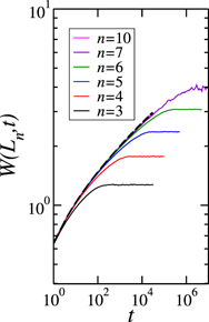
Figure 4. The surface width generated using the relaxation model in (3, 3) flower network of various generations, plotted on a double-logarithmic scale. The solid lines are for the Monte Carlo data and the dashed line is 1.17t0.094(1–0.477t−0.23).
Download figure:
Standard image High-resolution imageWe also estimated the exponent β by an alternative method of using the effective exponent, given by

The roughness exponent was also estimated in a similar way, defining

Substituting equations (16) for (17), one gets βeff = β + c t−Δ + ⋯ . Therefore, βeff should approach the exponent β as t−Δ → 0. Figure 5(a) shows βeff against t−Δ; the intercept on the ordinate gives the value β = 0.095(9). Similar analysis for αeff yielded α = 0.202(9), as shown in figure 5(b). The dynamic exponent z is obtained as z = α/β ≈ 2.13. It should be noted that this value of z is consistent with the fractal dimension dw = 2 of random walks in the (3, 3) flower network. The estimated values are comparable with the predictions in equation (13), i.e. β = 0.0923, α = 0.185, and z = 2.0. The deviations are fairly small (less than 10%), suggesting that equation (13) describes the exponents fairly well.
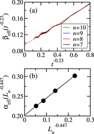
Figure 5. Plot of the effective exponents for the (3, 3) flower network. (a) shows βeff of n = 7, 8, 9, and 10, and (b) αeff of n = 3, 4, 5, and 6. The dashed line in (a) is 0.127t−0.23 + 0.095 and that in (b) is  .
.
Download figure:
Standard image High-resolution imageThe scaling function of W(Ln , t) can be written, considering the correction term, as

where g(x) is the scaling function with g(x) = const. for x ≫ 1. Figure 6 represents the scaling plot using α = 0.202 and z = 2.13; the data show good collapse in the large x limit. We also monitored the surface width for the (2, 3) flower network and repeated the same procedures to estimate both β and α.

Figure 6. Scaling plot of the surface width of the relaxation model in (3,3) flower network, using α = 0.202, e' = −0.917, Δ' = 0.391, and z = 2.13.
Download figure:
Standard image High-resolution imageThe numerical results, together with the results from a (2, 3) flower network, are summarized in table 1. Even though there are some corrections to scaling, the surface width shows power-law behavior for both (2, 3) and (3, 3) flower networks, where the exponents are consistent with equation (13).
Table 1. Exponents for various u v flower networks.
| Predictions by equation (13) | Numerical estimates | ||||||||
|---|---|---|---|---|---|---|---|---|---|
| (u, v) | ds | df | γ | β | α | z | β | α | z |
| (2, 2) | 2 | 2 | 3 | 0 | 0 | 2 | 0 | 0 | 2.11(10) |
| (2, 3) | 1.80 | 2.32 | 3.32 | 0.051 | 0.132 | 2.58 | 0.052(5) | 0.136(9) | 2.62(10) |
| (3, 3) | 1.63 | 1.63 | 3.59 | 0.092 | 0.185 | 2 | 0.095(9) | 0.202(9) | 2.13(9) |
3.3. The roles of heterogeneity in the degree distribution
To find the roles of heterogeneity in the degree distribution, we introduce a new quantity  , where ⟨⟩ represents the sample average. Actually δh(x, t) remains zero and is independent of position for the Family model in the case of both regular lattice and Sierpinski gasket substrates, where P(k) is a delta function. Because the deposited particle can diffuse a step to the site of lower height, the height of the hub sites has a greater chance to be higher than the average height
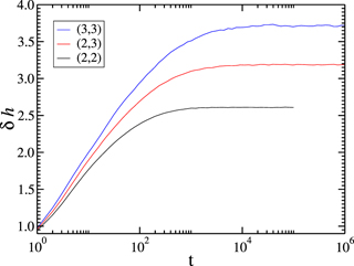
  due to the larger degrees. We expect that δh(x, t) of the hub site is positive and grows with time. The numerical result of δh(t) for the hub site for various (u, v) flower networks is shown in figure 7. δh(t) for the maximum hub site grows with t and becomes saturated at an order of Ws(L). In the EW equation, one expects δh(x, t) = 0 to be independent of position. The Family model in the heterogeneity of the degree distribution has different characteristics of δh(x, t) ≠ 0 in comparison with δh(x, t) = 0 of the EW equation. This heterogeneity may produce a quenched noise η'(x) effectively with non-zero δh(x, t). Actually, the Family model can be mapped to the random deposition model with the coarse-grained height of domain
  .
.
Figure 7. The numerical result of δh(t) for the maximum hub-site of the sixth generation for the (2, 2), (2, 3), and (3, 3) flower networks.
Download figure:
Standard image High-resolution image
Assume that the correlation length ξ grows as ξ(t) ∼ t1/z
. Within the area  , the fluctuation of the coarse-grained height follows
  due to the central limit theorem [24]. With W2(t) ∼ t2β
, it becomes
due to the central limit theorem [24]. With W2(t) ∼ t2β
, it becomes  , so we get
  in the mean field limit. The relation of equation (13) comes from the random deposition model of the coarse-grained height with the assumption that the coarse-grained disorder from the heterogeneity of the degree distribution becomes irrelevant. γ = 3 is a special case with ds = 2 and ⟨k2⟩ becomes infinite, where the central limit theorem for the disorder may break down. However for γ > 3, ⟨k2⟩ becomes finite and shows coarse-grained disorder due to the heterogeneity distribution becoming irrelevant as ξ grows. We think this is the reason why the width of (2, 3) and (3, 3) flower networks follows the power-law behavior of equation (13), with long initial crossover regime due to finite fluctuation of k.
4. Summary and conclusions
We studied a surface growth model with relaxation on fractal scale-free networks numerically. The mean square surface width was calculated for various system sizes as a function of time t, and the growth and roughness exponents were obtained. The results from the (2, 2) flower network was found to be distinct from those of the (2, 3) and (3, 3) flower networks. Note that γ = 3 for the (2, 2) flower network and γ > 3 for both (2, 3) and (3, 3) networks. For the (2, 2) flower network, the spectral dimension is ds = 2, and both the surface width and saturated width exhibited logarithmic divergences against time and system size, respectively. For the (3, 3) and (2, 3) flower networks, ds < 2, and both W2(L, t) and  increase as the power-law behaviors having finite time and size corrections with positive values of β and α. We speculate that these corrections may come from the inhomogeneity of the number of links such as the hub effect of the networks, where ⟨k2⟩ is finite. These results are consistent with the predictions of the fractional EW equation, in which the growth exponent β = 0 if ds = 2 and β > 0 if ds < 2. Actually, the Family model is mapped into the random deposition model with the coarse-grained height, and the results of equation (13) are obtained alternatively. On the other hand, in an earlier work [15], it was found on a complex scale-free network that Ws(N) grows logarithmically with N if the degree exponent γ < 3, and
  becomes constant if γ > 3. These observations, particularly the latter, are not consistent with our results from the (u, v) flower networks. Therefore, the surface growth phenomena in the (u, v) flower networks (fractal, scale-free and not small world) are distinct from the growth in complex scale-free (non-fractal and small world) networks, and they depend on the structures of the complex networks. The growth in the (u, v) flower network rather appears to be controlled by the spectral dimension ds.
Acknowledgments
I would like to thank S W Kim and S J Kim for much mathematical help. This research was supported by a grant from the National Research Foundation of Korea (NRF-2020R1A2C1003971).