

Abstract
Photoacoustic tomography (PAT) has become a fast-evolving biomedical imaging modality in recent years. In PAT, image reconstruction is a critical step to produce high-quality photoacoustic images from raw photoacoustic signals. To date, algorithms based on back projection are the most widely used image reconstruction techniques due to their simplicity and computational efficiency. However, images reconstructed by back projection contain negative values, especially at the edge of photoacoustic sources, which have no physical meaning and are essentially undesired artifacts. In this work, we study the formation mechanism, fundamental causes and removal strategies of the negativity artifacts in back-projection-based PAT. Our results show that limited detector bandwidth and limited view angle are two fundamental causes of negativity artifacts. When the bandwidth of a detector is limited, back-projection signals will be distorted as a result of the loss of frequency contents and negativity artifacts thus appear. When the view angle of the detector is limited, photoacoustic signals propagating in three-dimensional space will be partially lost, resulting in negativity artifacts. Post-processing strategies, such as envelope detection and forced zeroing can be used to remove the negativity artifacts but may cause problems. Since negativity artifacts are a common image quality degradation factor in PAT, understanding their characteristics may expedite the development of novel artifact-removal techniques and artifact-free image reconstruction algorithms, which are of importance to correct image interpretation and quantitative imaging.
Export citation and abstract BibTeX RIS

Original content from this work may be used under the terms of the Creative Commons Attribution 4.0 license. Any further distribution of this work must maintain attribution to the author(s) and the title of the work, journal citation and DOI.
1. Introduction
Benefitting from the excellent absorption contrast of optical imaging and the superb spatial resolution of deep-tissue ultrasound imaging, photoacoustic tomography (PAT) is a non-invasive hybrid biomedical imaging modality and has unique applications in a range of biomedical fields [1], such as cell biology [2–4], neurology [5, 6], oncology [7–9], rheumatology [10], ophthalmology [11, 12] and surgical navigation [9, 13]. PAT is principally based on the photoacoustic effect discovered by Alexander Graham Bell in 1880 [14], which describes energy conversion from light into acoustic waves. In PAT, pulsed light is used to illuminate biological samples and excite ultrasound waves, which are then recorded by ultrasound detectors and are further used to recover initial pressure distributions using image reconstruction algorithms. Image reconstruction plays an important role in PAT imaging. State-of-the-art image reconstruction algorithms mainly fall into two groups: iterative reconstruction and analytical reconstruction. Iterative reconstruction aims to find numerical solutions from a set of algebraic equations through an iterative process [15, 16], while the analytical reconstruction recovers original images by inverting the Radon transform [17, 18]. Although iterative reconstruction algorithms can produce enhanced image quality when photoacoustic projection data are limited, they are not as widely used as analytical reconstruction algorithms, especially in demanding applications such as real-time imaging and three-dimensional (3D) imaging, due to high computational cost.
The most widely known analytical reconstruction techniques for PAT are the back-projection (BP) algorithms [18, 19], which are mathematically based on the direct inversion of the circular or spherical Radon transform. Different versions of the BP algorithms have been reported [17–21]. Kruger et al first proposed an approximate BP reconstruction approach analogous to that used in x-ray computed tomography (CT) in 1995 and demonstrated its effectiveness through experiments [20]. Xu et al developed a rigorous BP reconstruction algorithm for spherical detection geometry in 2002 [21] and soon afterward extended it to more general cases, including spherical, cylindrical and planar detection geometries [18]. Moreover, Finch et al derived an exact BP reconstruction formula from spherical means over spheres centered on the boundary of the measurement geometry [19]. These pioneering works have enabled the BP algorithms to become a powerful image reconstruction approach in PAT. However, images reconstructed by BP contain negative values, especially at the edge of the targets. Since PAT images represent the initial pressure of biological tissues, negative pixel values are not physically meaningful and are essentially undesired artifacts, which may cause problems for image interpretation and quantitative PAT imaging [22, 23].
The presence of negativity artifacts in BP-based image reconstruction has already been noticed by the photoacoustic imaging community [16] and in our previous work [24]. However, no studies have been conducted yet to investigate their causes and impact. In this work, we analyze the formation mechanism of the negativity artifacts in BP-based photoacoustic image reconstruction and investigate the leading causes of the artifacts, including limited detector bandwidth and limited view angle. Two straightforward post-processing techniques, i.e. envelope detection and forced zeroing, are adopted to suppress the artifacts and their performances are evaluated through simulation and experiments.
2. Negativity artifacts in BP-based photoacoustic image reconstructions
2.1. BP-based photoacoustic image reconstruction and the ideal PSF
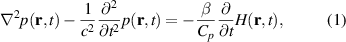
The generation and propagation of photoacoustic signals  under the condition of thermal confinement in lossless homogenous media are governed by the following photoacoustic wave equation:
where  is the heating source, representing the energy deposited in the tissue per unit volume per unit time, c is the speed of sound, β is the isobaric thermal volume expansion coefficient and Cp
denotes the specific heat capacity at constant pressure. Under the condition of stress confinement, the duration of the laser pulse is much shorter than the time it takes sound to travel across the heated region. The heating function can be decomposed as
is the heating source, representing the energy deposited in the tissue per unit volume per unit time, c is the speed of sound, β is the isobaric thermal volume expansion coefficient and Cp
denotes the specific heat capacity at constant pressure. Under the condition of stress confinement, the duration of the laser pulse is much shorter than the time it takes sound to travel across the heated region. The heating function can be decomposed as  , where
  is the energy deposited in the tissue per unit volume and δ(t) is the Dirac delta function. As a result, the initial acoustic pressure
  at the position
  can be written as:

where Γ is the Gr eneisen coefficient, a dimensionless constant that represents the efficiency of the conversion of heat energy to pressure. By solving equation (1) using Green's function, the acoustic pressure
  recorded by a detector at location
  , as depicted in figure 1, can be written as:
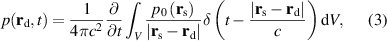
where dV is a 3D volume element at  . This equation mathematically represents the spherical Radon transform and suggests that the initial acoustic pressure
  in a small tissue volume at
  linearly contributes to the recorded acoustic pressure
  . However, the contribution falls as the inverse of the distance between the source and the detector, i.e. as 1/
 .
.
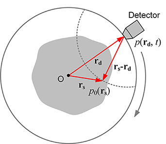
Figure 1. Schematic showing the signal detection and image reconstruction geometry in PAT.
Download figure:
Standard image High-resolution imageImage reconstruction in PAT aims to recover the initial acoustic pressure distribution  from measured photoacoustic signals
  by reverting the spherical radon transform in equation (3). To achieve this, several analytical inversion approaches have been proposed [17–21]. One of the most well known is the BP algorithm proposed by Xu et al [18], which reconstructs the initial pressure distribution
  through the following inversion formula:
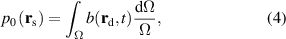
where the BP term is
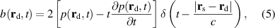
Ω is the entire solid angle covered by the detection surface (Ω = 2π for the infinite planar geometry and Ω = 4π for the spherical and cylindrical geometries) and dΩ is the solid angle subtended by the element dσ of the detection surface and can be written as
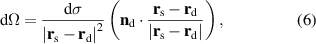
where  denotes the unit normal vector of the detector surface pointing to the region of interest. It has been proven that the impulse response of the BP reconstruction algorithm for unbounded planar, unbounded cylindrical and closed spherical imaging geometries is a Dirac delta function and the point spread function (PSF) takes the form [18] of:

where  and
and  represent the locations of the point of interest and the point source, respectively. This equation suggests that, under ideal circumstances, the BP algorithm can achieve theoretically exact reconstruction of the point source without causing negativity artifacts.
2.2. Negativity artifacts
The conclusion that the impulse response of the BP algorithm is a delta function is only valid under ideal circumstances, such as unbounded planar, unbounded cylindrical and closed spherical imaging geometries and infinite detector bandwidth. Such conditions, however, can never be fully met in real experiments. The deviation from these ideal conditions contaminates the PSF and eventually degrades the image quality. The presence of negativity artifacts at the edge of photoacoustic sources is a typical manifestation of image degradation.
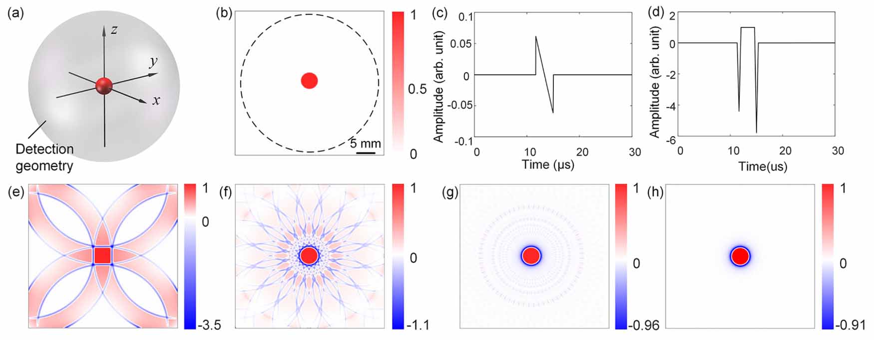
To understand the formation process of negativity artifacts in BP-based image reconstruction, a group of simulations was performed. In this example, the photoacoustic source is a unit-intensity spherical absorber with a diameter of 5 mm located at the origin and the detection geometry is a spherical surface with a diameter of 40 mm, as shown in figure 2(a). Figure 2(b) is the cross section of figure 2(a) in the x–y plane showing the spherical absorber reduces to a disk and the spherical detection geometry becomes a circle. Figures 2(c) and (d) show the recorded approximately N-shaped signal  by a bandwidth-limited ((0, 4) MHz) detector located on the circle and the BP signal
  used for image reconstruction, respectively. Figures 2(e)–(h) are the reconstructed images of the disk using 4, 16, 64, and 256 detectors uniformly distributed on the detection circle, respectively. Although the recovered disk images more and more resemble the original one as the number of detectors increases, they always contain negative values or negativity artifacts at the edge of the source, which does not disappear even with many detectors. The negativity artifacts do not arise from the negative components of the N-shaped signals but from the pair of negative wings of the BP signals in figure 2(d).

Figure 2. Formation of negativity artifacts in BP-based photoacoustic image reconstruction. (a) Schematic showing a unit-intensity spherical absorber (diameter: 5 mm) and a spherical detection geometry (diameter: 40 mm). (b) x–y cross section of (a) showing a disk in the center and a detection circle around it. (c) N-shaped photoacoustic signal recorded by a bandwidth-limited ((0, 4) MHz) detector located on the detection circle in (b). (d) BP signal obtained from (c) using equation (5). (e)–(h) Reconstructed disk images using 4, 16, 64, and 256 detectors uniformly distributed on the detection circle, respectively. Negativity artifacts are displayed in blue.
Download figure:
Standard image High-resolution imageThe image reconstruction results shown in this example do not support the exact reconstruction theory presented in equation (7). The fundamental cause is the aforementioned deviation from the ideal imaging conditions. In this simulation, the detector bandwidth is not infinite but has been restricted to (0, 4) MHz. Limited bandwidth causes the detectors only to respond to a certain frequency range of the broadband photoacoustic signals and eventually introduces negativity artifacts. Moreover, the detection surface only encloses the target in a two-dimensional (2D) plane (2π radian view angle) rather than 3D space (4π steradian view angle). Since photoacoustic signals propagate in 3D space, the vast majority of the signals from the target are lost. In the following section, we quantitatively investigate the impact of the detector bandwidth and view angle on the formation of the negativity artifacts. It is worth mentioning that limited bandwidth and limited view angle will result in positive artifacts and negative artifacts simultaneously. However, negative artifacts are usually more prominent and are the focus of this work.
3. Causes of negativity artifacts
3.1. Limited detector bandwidth
To investigate the impact of bandwidth on negativity artifacts, we assume that the signal detection geometry is a closed sphere and the bandwidth is the only impacting factor. The study starts with the bandwidth-limited PSF. In [25], Xu et al developed a PSF formula incorporating the effect of detector bandwidth, which can be written as:
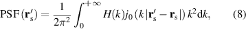
where k = 2πf/c is the wavenumber, f is the ultrasound frequency, j0 is the zeroth-order spherical Bessel function of the first kind, H(k) is the frequency response of the ultrasound detector and  is the distance from the point source
  to the point of interest
  . The PSF expressed in equation (8) applies to the planar, cylindrical and spherical detection geometries.
Specifically, if the detector has a flat frequency response over the entire frequency band, i.e. H(k) = 1 when  , equation (8) reduces to a Dirac delta function, the same as equation (7). However, this case may never happen in real experiments because ultrasound detectors cannot respond beyond a maximum frequency, which we call the upper cutoff frequency k2. Assume that H(k) = 1 within the band (0, k2) and H(k) = 0; otherwise, equation (8) can be simplified as:
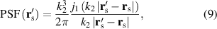
where j1 is the first-order spherical Bessel function of the first kind. Real ultrasound detectors not only have an upper cutoff frequency k2 but also a lower cutoff frequency k1. Assume that H(k) = 1 within the bandwidth  and H(k) = 0; otherwise, equation (8) can be further written as:
Equations (9) and (10) show that the PSFs of a bandwidth-limited detector no longer converges to a Dirac delta function but are broadened as a result of the spherical Bessel function. Since the spherical Bessel functions have negative side lobes, the PSF of a bandwidth-limited detector contains negativity artifacts in principle. As an example, figures 3(a) and (b) show the PSFs of two ultrasound detectors with bandwidths of (0, 5) MHz and (4, 10) MHz, respectively, while figure 3(c) illustrates their center profiles. Ringing negativity artifacts due to limited bandwidth are visible in the PSFs, which eventually result in negative values in the final reconstructed images.

Figure 3. The effect of detector bandwidth on the PSF. (a) PSF of an ultrasound detector with a bandwidth of [0, 5] MHz. (b) PSF of an ultrasound detector with a bandwidth of [4, 10] MHz. (c) Center profiles of the PSFs in (a) and (b).
Download figure:
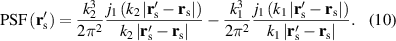
Standard image High-resolution imageFurthermore, we studied the impact of bandwidth on the negativity artifacts in photoacoustic images reconstructed by BP. The numerical phantom used in this example is a unit-intensity spherical absorber located at the origin and the detection geometry is a closed spherical surface, similar to the configuration in figure 2(a). In this case, the diameters of the spherical absorber and the spherical detection surface are 2 and 30 mm, respectively. Signals from the absorber are first captured by 32 768 bandwidth-limited detectors (center frequency fc = 3 MHz) evenly distributed on the spherical detection surface in 3D space and then used for image reconstruction. Figures 4(a)–(d) show the recorded signal by a detector with a fractional bandwidth of 100%, its frequency spectrum, the BP signal and the final reconstructed image, respectively. From these results, we may draw several conclusions. First, due to limited detector bandwidth, the recorded time-domain signal (figure 4(a)) loses a significant portion of the frequency contents of the original signal (figure 4(b)) and is no longer N-shaped. Second, the distorted time-domain signal yields an inaccurate BP signal (figure 4(c)), which differs greatly from the theoretical BP signal, especially at the edge. Third, when back-projected, the inaccurate BP signal produces a distorted initial pressure image (figure 4(d)) with many negativity artifacts at the edge. As a comparison, figures 4(e)–(h) show another group of simulation with similar parameter settings except that the fractional bandwidth of the detector is expanded to 500%, i.e. bandwidth ranging from 0 to 15 MHz. Bandwidth expansion greatly eases the problem of frequency contents loss and minimizes the distortion of the recorded signal, which in turn yields approximately perfect images having significantly fewer negativity artifacts. To quantify the impact of bandwidth on the amplitude of the negativity artifacts in this example, the fractional bandwidth of the detectors was tuned from 100% to 1000%. Figure 5 shows the evaluation results, which suggests that the amplitude of the negativity artifacts decreases with the increase of the bandwidth, although the improvement is not very significant when the bandwidth is broad enough. Limited detector bandwidth is a fundamental cause of negativity artifacts in BP-based photoacoustic image reconstruction. Bandwidth expansion is helpful to mitigate the problem.
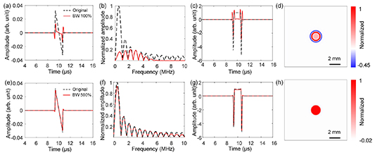
Figure 4. Narrower detector bandwidth yields more significant negativity artifacts in BP-based image reconstruction. The numerical phantom used in this example is a unit-intensity spherical absorber located at the origin and the detection geometry is a closed spherical surface, similar to the configuration in figure 2(a). (a), (e) Comparisons of the theoretical N-shaped signal (dashed black line) and the recorded signals (solid red) by detectors with bandwidths of 100% and 500%, respectively. (b), (f) Comparisons of the Fourier spectra of the N-shaped signal and the signals recorded by detectors with bandwidths of 100% and 500%, respectively. (c), (g) Comparisons of the theoretical BP signal with those at 100% and 500% bandwidths, respectively. (d), (h) Center cross sections of the final reconstructed images at 100% and 500% detector bandwidth, respectively.
Download figure:
Standard image High-resolution image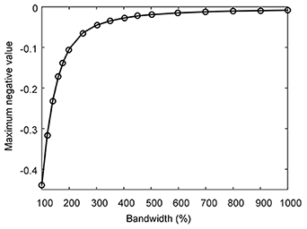
Figure 5. Broader detector bandwidth produces fewer negativity artifacts in BP-based image reconstruction. Data points on the plot represent the maximum negative amplitude of PA images reconstructed using PA signals at corresponding detector bandwidths. The simulation settings used here are the same as those in figure 4.
Download figure:
Standard image High-resolution image3.2. Limited view angle
Besides detector bandwidth, the limited view angle is another fundamental factor that gives rise to negativity artifacts. Theoretically, photoacoustic signals generated from the source will not be confined in a particular plane or direction but will propagate in 3D space. Collecting signals from all view angles helps perfect image reconstruction. However, real experiments may never fulfill this requirement, which unavoidably causes negativity artifacts. To investigate the impact of detector view angle on negativity artifacts, we assume that the detector bandwidth is infinite and the view angle is the only impacting factor in the following discussion. Since the derivation of analytical PSF formulas for imaging geometries with limited covering angle is challenging, numerical simulation is adopted to study the impact of detector view angle on the negativity artifacts.
A multi-sphere phantom designed to reflect the distribution of negativity artifacts under different detection view angles is shown in figure 6(a). It consists of nine spherical absorbers with unit intensity. Eight of the absorbers with diameters uniformly varying from 1 to 2 mm are evenly distributed on a circle with a radius of 5 mm while the ninth one, having a diameter of 1.6 mm, is seated at the origin. Figures 6(b) and (c) give the cross sections of the phantom in the x–z and x–y planes, respectively.
Figure 6. A numerical phantom consisting of nine spherical absorbers is used to demonstrate the characteristics of the negativity artifacts in BP-based image reconstruction. (a) 3D view. (b) x–z plane. (c) x–y plane. Eight absorbers with diameters uniformly varying from 1 to 2 mm are evenly distributed on a circle with a radius of 5 mm while the ninth one, having a diameter of 1.6 mm, is seated at the origin. All absorbers have a unit intensity.
Download figure:
Standard image High-resolution imageTo study the impact of detector view angle on the characteristics of negativity artifacts, the multi-sphere phantom is imaged by three open spherical detection segments, as shown in figures 7(a)–(c). The three spherical detection segments have the same geometric radius (15 mm) and equal detector distribution density (32 768 point detectors evenly distributed over the entire spherical surface) but different surface areas or solid view angles (π, 1.5π and 2π steradian for figures 7(a)–(c), respectively). The frequency response of each detector was set to approximately full bandwidth to minimize its impact on the results. The imaging results of the x–z cross section of the phantom at view angles of π, 1.5π and 2π are shown in figures 7(d)–(f), respectively. It can be seen that negativity artifacts appear in all three x–z cross-section images as a result of the limited angle of view but their distribution and amplitude at 2π are significantly less than those at smaller view angles. This indicates that a larger view angle can produce better image quality and suppress the negativity artifacts more efficiently. The imaging results of the x–y cross sections at view angles of π, 1.5π and 2π are shown in figures 7(g)–(i). The distribution and amplitude of the negativity artifacts look different from those in the x–z cross sections but obey the same rule. The difference lies in that the artifacts, in this case, are much fewer. This is because the x–y cross section of the photoacoustic source is approximately parallel to the detection surfaces, which satisfies the visibility condition [24, 26] in PAT and can achieve better signal detection and image reconstruction. Nevertheless, the conclusion that a larger view angle improves the image quality and produces fewer artifacts still holds. Note that we do not perform simulations for view angles greater than 2π ( ) because their artifacts are exactly opposite in sign to those at 4π − Ω under the condition of exact image reconstruction (equation (7)).
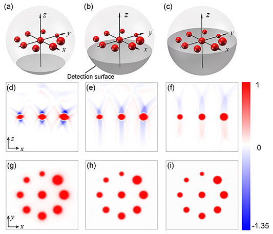
Figure 7. The effect of limited view angle on the amplitude and distribution of the negativity artifacts. (a)–(c) Photoacoustic signals generated from the multi-sphere phantom are detected by three spherical detection segments (radius: 15 mm) with solid view angles of π, 1.5π and 2π, respectively. (d)–(f) Corresponding reconstruction results of the cross section in the x–z plane. (g)–(i) Corresponding reconstruction results of the cross section in the x–y plane.
Download figure:
Standard image High-resolution imageThe above simulation demonstrates that the view angle of the detection geometry needs to be expanded to reduce the negativity artifacts for the spherical detection geometry. To study how detection geometry affects the distribution and amplitude of the negativity artifacts, we performed another set of simulations using planar, cylindrical and spherical geometries with finite surface areas, a practical situation in experiments. Figures 8(a)–(c) show the arrangements of the multi-sphere phantom and the three detection geometries, where the planar surface is located 12 mm away from the x–y plane, and the cylindrical surface, as well as the spherical detection surface, is located at the origin. For comparison, all three geometries have the same number of point detectors (32 768) and an approximately equal detection area (figure 8(a) 150 mm × 150 mm; figure 8(b) base radius: 35 mm, height: 100 mm; figure 8(c) radius: 42 mm). The planar and cylindrical surfaces are thus bounded while the spherical surface is closed with respect to the photoacoustic source. The frequency response of each detector was set to approximately full bandwidth to minimize its impact on the results. Figures 8(d)–(f) present the reconstruction results of the cross section of the phantom in the x–z plane while figures 8(g)–(i) show the results in the x–y plane. From these results, we may conclude as follows. First, the spherical detection geometry produces invisible negativity artifacts and the best image quality among the three, as shown in figures 8(f) and (i). This is easy to understand because the spherical detection surface is closed and strictly satisfies the exact image reconstruction condition required by BP. Second, the bounded planar detection surface yields significantly fewer negativity artifacts in the x–y plane (figure 8(g)) compared with the result produced by the cylindrical surface (figure 8(h)). This is because the photoacoustic signals emanating from the source in the x–y plane can be largely captured by the planar detector (the normal of the source intersects with the detector surface) and, therefore, the source can be reasonably reconstructed [24, 26]. However, this is not true for the cylindrical detection surface. Third, the bounded cylindrical detection surface yields fewer negativity artifacts in the x–z plane (figure 8(e)) compared with the result produced by the planar surface (figure 8(d)). This is again due to the amount of signal collected by the detection surface and can be explained using the visibility condition in [24, 26]. This example illustrates that view angle plays an important role in the generation of negativity artifacts in different detection geometries.
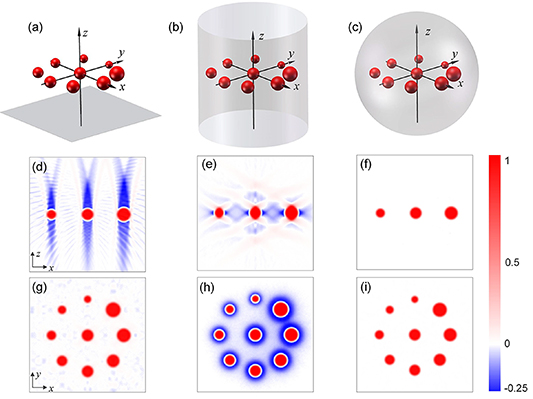
Figure 8. Signal detection and image reconstruction by three commonly used detection geometries in PAT. (a)–(c) Schematic showing the planar, cylindrical (without the top and bottom) and spherical recording surfaces and the multi-sphere phantom. All three recording surfaces have the same number of detectors and an approximately equal detection area. (d)–(f) Corresponding x–z cross sections of the reconstructed images by BP. (g)–(i) Corresponding x–y cross sections of the reconstructed images by BP.
Download figure:
Standard image High-resolution imageIn all of the numerical experiments presented so far, we used a fixed detector density, that is, 215 (32 768) point detectors uniformly distributed over the entire spherical surface to perform the investigation. In principle, the number of detectors should be infinite because the signal-collecting surface is continuous and the detector is assumed to be a point. Decreasing the number of detectors is equivalent to decreasinge the solid view angle, which may produce negativity artifacts. Figure 9 presents a simulation reflecting the relationship between the amplitude of the negativity artifacts and the number of detectors under the same parameter settings as figure 8(c). When the number of detectors is small, significant negativity artifacts are produced, which, however, can be greatly improved by increasing the number of detectors. The number of detectors, 32 768, used in this study produces negligible negativity artifacts in this case and is, therefore, sufficient for this study.

Figure 9. Impact of detector number on the negativity artifacts. The simulation settings used in this example are the same as those in figure 8(c) except that the number of detectors is kept varying to study its impact on the significance of the negativity artifacts.
Download figure:
Standard image High-resolution image4. Negativity artifact removal
To produce photoacoustic images free from negativity artifacts, infinite detector bandwidth and ideal detection geometries are required, which, however, can never be fulfilled in real scenarios. Physical piezoelectric ultrasound detectors have very limited fractional bandwidth, typically less than 100%, which may cause significant negativity artifacts (see section section 3.1). Detection geometries used in practical scenarios such as breast imaging have a limited angle of view and cannot be unbounded planar, unbounded cylindrical or closed spherical surfaces. Most detection geometries used in experiments are lines, arcs or circles, which visualize photoacoustic sources in a 2D plane and may cause significant artifacts.
To yield physically sound photoacoustic images, post-processing procedures removing the negative values might be necessary. Two common yet simple artifact-removal techniques, i.e. envelope detection and forced zeroing, are investigated in this study. The envelope detection method converts a bipolar photoacoustic image into a unipolar image by reverting its negative components and extracting the amplitude profile using methods, such as the Hilbert transform, which can be mathematically written as:

where ε denotes envelope detection and f and g are images before and after envelope detection. Details of the envelope detection method used in this paper for full-ring transducer array-based PAT can be found in [27]. The forced-zeroing method produces non-negative photoacoustic images by simply setting negative values of an image to zero, which can be formulated as:
We first tested the performance of the two post-processing approaches using a simple numerical disk phantom (diameter: 1 mm), shown in figure 10(a). Photoacoustic signals from the disk are collected by a circular detection geometry (diameter: 20 mm), which has 512 evenly spaced point ultrasound detectors. The point detectors have a center frequency of 1 MHz and a bandwidth of 100%. The forward-simulation process was performed using the k-Wave toolbox [28]. Figure 10(b) is the raw image reconstructed by BP, which contains significant negativity artifacts around the edge of the disk. Applying the envelope-detection and forced-zeroing post-processing methods, images free from negativity artifacts are obtained, as shown in figures 10(c) and (d), respectively. The image processed by envelope detection (figure 10(c)) has been significantly blurred and widened while the image processed by forced zeroing (figure 10(d)) is not blurred but visually smaller than the original disk. Figure 10(e) illustrates the amplitude profiles of the original disk, the disk reconstructed by BP and the disks processed by envelope detection and forced zeroing. We can see that envelope detection blurs and widens the image due to its low-pass filtering nature. Forced zeroing produces a visually smaller image because the main lobe of the image reconstructed by BP is smaller than the ground truth, which is the result of signal loss due to limited bandwidth and limited angle of view.
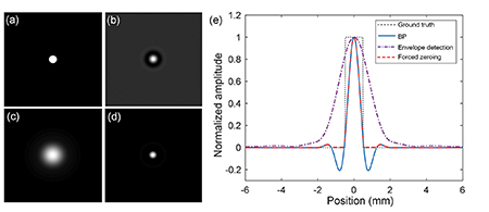
Figure 10. Performance comparison of the envelope-detection and forced-zeroing methods using a simple disk phantom. (a) Original image of the disk with a diameter of 1 mm. (b) Image reconstructed by BP. (c) Image reconstructed by BP with envelope detection. (d) Image reconstructed by BP with forced zeroing. (e) Comparison of the central amplitude profiles in (a)–(d).
Download figure:
Standard image High-resolution imageWe further numerically and experimentally evaluated the performance of the two post-processing algorithms using tissue-mimicking phantoms. In the numerical simulation, a designed blood vessel phantom (figure 11(a)) is used as the photoacoustic source, whose signals are collected by a circular detection geometry (diameter: 25 mm) with 512 evenly spaced point ultrasound detectors. In the experimental evaluation, a 3D-printed blood vessel phantom submerged in water (figure 11(e)) is regarded as the photoacoustic source, whose signals are collected by an ultrasound detector (V303, Olympus) scanning in a circular trajectory (diameter: 107 mm) around the source for 512 steps. The ultrasound detectors used in the simulation and experiments have the same center frequency of 1 MHz and the same −6 dB bandwidth of 60.5%. Figures 11(b) and (f) present the raw images reconstructed by BP corresponding to figures 11(a) and (e), respectively, where significant negativity artifacts are present at the edge of the image in both the simulation and experiment. Figures 11(c) and (g) are processed results of the raw BP images by envelope detection. The processed images have been blurred and widened as expected. Figures 11(d) and (h) are processed results of raw BP images by forced zeroing. The processed images have a much cleaner background and possess a higher resolution. The analyses are valid both for the simulation results and the experimental results, although the latter exhibit more significant negativity artifacts (figure 11(f)), which may be caused by non-ideal factors, such as narrower detector bandwidth, finite detector aperture, acoustic attenuation, etc

Figure 11. Performance comparison of the envelope-detection and forced-zeroing methods using blood vessel phantoms. (a), (e) Numerical and 3D-printed blood vessel phantoms, respectively. (b), (f) Corresponding reconstructed raw images. See the text for the simulation and experimental settings. (c), (g) Results of (b) and (f) processed by envelope detection, respectively. (d), (h) Results of (b) and (f) processed by forced zeroing, respectively.
Download figure:
Standard image High-resolution imageTo test the performance of the two post-processing methods more realistically, we performed an in vivo imaging experiment on a human finger, as shown in figure 12(a). The PA signals generated from the finger were detected by a circular detection geometry (diameter: 50 mm) with 256 evenly distributed ultrasound detectors (center frequency: 7 MHz; −6 dB bandwidth: 80%). Figure 12(b) is the image reconstructed by BP, which contains significant negativity artifacts at the edges of the blood vessels. Figures 12(c) and (d) are the processed results of figure 12(b) by envelope detection and forced zeroing, respectively. As expected, envelope detection blurs and widens the blood vessels (figure 12(c)), while forced zeroing produces an image with a cleaner background and sharper borders (figure 12(d)).

Figure 12. In vivo human finger imaging experiment showing the performance of the envelope detection and forced zeroing methods. (a) Photograph of a human finger with a red dashed line indicating the imaging cross section. (b) Corresponding raw bipolar image reconstructed by BP. See the text for the experimental settings. (c) Result of (b) processed by envelope detection. (d) Result of (b) processed by forced zeroing.
Download figure:
Standard image High-resolution image
As mentioned above, the envelope detection method gives physically meaningful images by inverting negative values, which are regarded as a part of the final image. Therefore, images processed by this method will be more or less blurred or widened, depending on the amplitude and distribution pattern of the negativity artifacts. For images with significant negativity artifacts such as the one in figure 8(d), this method may lead to resolution degradation. On the other hand, the forced-zeroing method produces non-negative images by simply discarding their negative values, which is simple, effective and easy to implement. However, in some scenarios, it may result in the loss of source details, which are overwhelmed by the negativity artifacts [27, 29, 30]. In such cases, the envelope-detection method may retain more useful information about the source but at the expense of blurring and broadening it. One should be aware of the benefits of each method as well as their potential problems when applying them to remove negativity artifacts.
5. Discussion and conclusion
This study is carried out based on the assumption that the acoustic media is lossless and homogenous, which means no acoustic attenuation and refraction are considered in the aforementioned analyses. Violation of these conditions in practical scenarios will result in negativity artifacts. Acoustic attenuation is a frequency-dependent physical process, in which higher-frequency ultrasound waves lose energy faster than lower-frequency waves while propagating. Ultrasound signal received by a detector is essentially the low-pass filtered version of the original one, which will lead to negativity artifacts based on the bandwidth analysis in section 3.1. Non-homogenous acoustic media may also introduce negativity artifacts. This is because the BP process determines the position of the photoacoustic source based on the assumption that the sound speed in tissue is constant and ultrasound waves propagate along a straight line. Real biological tissues have heterogeneous sound speed distributions and refract ultrasound waves at interfaces [31], which result in incorrect estimation of the location of the source and lead to negativity artifacts. Furthermore, noise could lead to negativity artifacts, which mainly concentrate on the background of the reconstructed images. The impact of signal-to-noise ratio on the negativity artifacts is not as significant as the impacts of limited bandwidth and limited view angle.
The discussed negativity artifacts occur in not only the BP algorithm but also other types of image reconstruction algorithms, such as time-reversal [32] and frequency-domain methods [33]. The conclusions regarding bandwidth and view angle drawn in this study also apply to these algorithms. Differently, iterative reconstruction algorithms could yield photoacoustic images free from negative values, even if the imaging scenarios are imperfect [30, 34]. This is because specially designed non-negative constraints, such as simple thresholding [34] or logarithmic regularization [30], are usually imposed on the objective function to suppress negative values. It has been suggested that iterative algorithms with non-negative constraints could produce better image qualities compared with analytical methods and unconstrained iterative methods. However, iterative algorithms are computationally expensive, which limits their practical applications, especially in real-time and 3D imaging.
In summary, we studied the formation mechanism, fundamental causes and removal strategies of negativity artifacts in BP-based PAT. Negativity artifacts present in photoacoustic images do not arise from the negative cycles of detected photoacoustic signals but from the negative components of BP signals. Fundamental causes of negativity artifacts include limited detector bandwidth and limited view angle. When the bandwidth of the detector is limited, recorded photoacoustic signals and BP signals will be distorted compared with theoretical ones as a result of the loss of frequency contents and negativity artifacts thus appear. When the view angle of the detector is limited, photoacoustic signals propagating in 3D space will be partially lost, resulting in negativity artifacts and imperfect image reconstruction. These analyses are general and apply to other types of image reconstruction algorithms. Envelope detection and forced zeroing are two common artifact-removal strategies, but one should be aware of their benefits and potential problems. Negativity artifacts are a common image quality degradation factor in PAT. This work is expected to help the photoacoustic imaging community better understand its characteristics and pave the way for the development of novel artifact-removal techniques and artifact-free image reconstruction algorithms.
Acknowledgments
National Natural Science Foundation of China (NSFC) (61705216); Natural Science Funds of Jiangsu Province of China (BK 20170826); Major Science and Technology Project of Anhui Province (18030801138); Research Fund of the Zhejiang Lab (2019MC0AB01); Research Fund of the Chinese Academy of Sciences (CAS); Research Fund of the Double First Class Initiative; Research Fund of the USTC Smart City Institute; Startup Fund of the University of Science and Technology of China (USTC).