Model of Continuous Random Cascade Processes in Financial Markets

Introduction

In financial time series, past coarse-grained measures of volatility correlate better to future fine-scale volatility than the reverse process. Such a causal structure of financial time series was first reported by Müller et al. [1]. Since then, the causal structure between time scales, the flow of information from a long-term to a short-term scale, was investigated empirically in financial markets; it has been supported by multiple studies [2, 3] as a stylized fact of financial time series [4]. The asymmetric flow of information resembles an energy cascade found in conditions of turbulence. In a developed turbulent flow, the energy injected from the outside at macroscopic spatial scales is transferred to smaller scales and finally dissipated as heat at microscopic spatial scales [5–9]. Gashghaie et al. investigated details of the self-similar transformation rule of the probability density function of price fluctuations and the nonlinear scaling law of the structure function (nth moment of fluctuations), signifying the multifractality of the time series, in their study of the time series of foreign exchange. They pointed out the similarity of price changes in the financial time series to the velocity difference between two spatial points in turbulence [10, 11]. The intermittency in turbulence is a phenomenon characterized by the sudden temporal change of the statistical feature of fluctuations and the spatial coexistence of large and small fluctuations. Such intermittency, which is frequently encountered in heterogeneous complex systems, is well known in financial markets as volatility clustering [4, 12]. Intermittency at each time scale produces a characteristic hierarchical structure designated as multifractality [8, 9].

In the developed turbulence, the process by which mechanically generated vortices on a macroscale deform and destabilize according to the Navier–Stokes equation and then split into smaller vortices is regarded as an energy cascade. A similar idea of modeling multifractal time series by a recursive random multiplication process from a coarse-grained scale to a microscopic scale has offered an attractive means of describing financial time series [13, 14]. Chen et al. verified the statistics of multiplier factors in the random multiplication process of turbulent flow by empirical studies using measured data and numerical experiments of Navier–Stokes equations [15]. Results show that the multiplier factors connecting two adjacent layers follow a Cauchy distribution in which all moments diverge and show that they are not independent. They show strongly negative correlation between the multiplier factors of adjacent layers. The authors verified the statistics of multipliers calculated backward from actual stock price fluctuations, finding a Cauchy distribution of multiplier factors and also the strongly negative correlation between the multiplier factors in financial markets. Results show that the discrete cascade model using the random multiplication process did not reproduce the statistical property of the multiplier factors. Therefore, as an alternative model, a discrete random multiplicative cascade process with additional additive stochastic processes [16–18], or a model formulated as the Fokker–Planck equation considering the cascade process as a continuous Markov process [19–23] was proposed. Those models have been applied to stock market or foreign exchange market data, yielding empirical results including the statistics of multipliers.

This study examines a continuous cascade model of volatility formulated as a stochastic differential equation including two independent modes of Brownian motion: one has multiplicative coupling with volatility; the other has additive coupling as in the discrete random multiplicative cascade process with additional additive stochastic processes described above. The model parameters are estimated by its application to the stock price time series. Numerical calculation of the Fokker–Planck equation derived from the stochastic differential equation is conducted using the estimated values of parameters resulting in successful reproduction of the pdf of the empirical volatility and the multifractality of the time series.

Materials and Methods

Continuous Random Cascade Model

Stochastic Differential Equation

These analyses examine the following wavelet transform of the variation of the logarithmic stock price denoted by $Z\left(t\right)=\text{log}S\left(t\right)/S\left(0\right),t\in \left[0,L\right]$:

where the function ψ is designated as the analyzing wavelet. When using the delta function $\psi \left(t\right)=\delta \left(t-1\right)-\delta \left(t\right)$ as the analyzing wavelet, the wavelet transform $W_{\psi }Z\left[u,s\right]=Z\left(u+s\right)-Z\left(u\right)$ is exactly the logarithmic return of the period s. Here, we use the second derivative of the Gaussian functions as

In general, by using the nth derivative of the function having asymptotic fast decay as the analyzing wavelet, one can remove the local trend of mth order $\left(m\le n-1\right)$ because the function is orthogonal to mth-order polynomials. For the second derivative of the Gaussian functions, the linear trends of $Z\left(t\right)$ with scale s have been eliminated in the wavelet transform $W_{\psi }Z\left[u,s\right]$.

In actual financial market, the price fluctuation is nonstationary and the volatility is not observable. The quantity used herein is the absolute value of the wavelet transform $x\left(\lambda \right)=\left|W_{\psi }Z\left[t_0,s\left(\lambda \right)\right]\right|$ for arbitrary $t_0$ as a volatility proxy, where we use the variable $\lambda =\text{log}L/s$. The quantity $x\left(\lambda \right)$ is thought to be a generalization of empirical volatility, whereas the wavelet transform $W_{\psi }Z[u,s]$ is exactly the absolute value of logarithmic return when we use $\psi \left(t\right)=\delta \left(t-1\right)-\delta \left(t\right)$.

The following stochastic equation is used to start.

In that equation, $B\left(\lambda \right)$ represents the Brownian motion. Equation 3 expresses that the value of the quantity $x\left(\lambda +d\lambda \right)$ at scale $\lambda +d\lambda$ is obtained stochastically from $x\left(\lambda \right)$ at just a slightly larger scale λ by multiplying the stochastic variable $W\left(\lambda ,\lambda +d\lambda \right)=e^{\sigma dB\left(\lambda \right)+\mu d\lambda }$. The stochastic multiplier $W\left(\lambda ,\lambda +d\lambda \right)$ follows a logarithmic normal distribution $LN\left(\mu d\lambda ,{\sigma }^{2}d\lambda \right)$ because $dB\left(\lambda \right)\sim N\left(0,d\lambda \right)$. One can derive the following stochastic differential equation using $dB{\left(\lambda \right)}^2=d\lambda$ as

The solution is obtained easily using Ito’s formula as [24].

The power law behavior of the qth moment $E\left[x{\left(\lambda \right)}^q\right]$ (qth structure function) as a function of scale s is proved by the solution of Eq. 5 as follows:

The multifractality of signal $Z\left(t\right)$ for which the wavelet transform follows the stochastic Eq. 4 is verified because the scaling exponent $\tau \left(q\right)=-\mu q-\frac{1}{2}{\sigma }^2{q}^2-1$ is a convex upward nonlinear function. However, in this model, the stochastic multiplier $W\left({\lambda }_2,{\lambda }_1\right)=x\left({\lambda }_2\right)/x\left({\lambda }_1\right)\left({\lambda }_2\le {\lambda }_1\right)$ linking two scales follows the logarithmic normal distribution $LN\left(\mu \left({\lambda }_1-{\lambda }_2\right),{\sigma }^2\left({\lambda }_1-{\lambda }_2\right)\right)$. It is independent of the multiplier $W\left({\lambda }_3,{\lambda }_2\right) \left({\lambda }_3\le {\lambda }_2\right)$ linking two adjacent scales. That result is contrary to the empirical results described in Introduction.

We introduce an additional additive stochastic process as we have done in the discrete cascade model. We first consider the following stochastic differential equation.

The equation is produced on the assumption that Brownian motions $d{B}_M\left(\lambda \right)$ and $d{B}_A\left(\lambda \right)$ are mutually independent. The first two terms correspond to Eq. 4. The origin of those random sources triggering volatility cascade in financial markets remains unclear.

To solve the stochastic differential Eq. 7, we consider the following stochastic differential equation:

which is the same as Eq. 4. Using the solution of Eq. 8

the solution of Eq. 7 is expressed as shown below:

Statistics of Multipliers

We have mentioned the statistics of multipliers in Introduction:

(1) The stochastic multiplier $W({\lambda }_2,{\lambda }_1)=x\left({\lambda }_2\right)/x\left({\lambda }_1\right) ({\lambda }_2\le {\lambda }_1)$ linking two different scales follows a Cauchy distribution.

(2) When considering the three scales ${\lambda }_1<{\lambda }_2<{\lambda }_3 (s_1>s_2>s_3)$, the adjacent multipliers $W\left({\lambda }_2,{\lambda }_1\right)=x\left({\lambda }_2\right)/x\left({\lambda }_1\right)$ and $W\left({\lambda }_3,{\lambda }_2\right)=x\left({\lambda }_3\right)/x\left({\lambda }_2\right)$ show strongly negative correlation.

Here, we show property (1) and infer the existence of correlation between adjacent multipliers under some reasonable approximations. The parameter ${\sigma }_M$ is an important model parameter for the signal to have multifractality. As presented in a later section, in spite of the importance, the value of the parameter ${\sigma }_M^2$ is small, about $0.02\text{ to }-0.03$ in stock markets, irrespective of the stock issue. To specifically examine the role of additional stochastic processes, we investigate the 0th-order approximation of small ${\sigma }_M$. When setting ${\sigma }_M=0$, the solution of Eq. 10 becomes

Therefore, the difference $\text{Δ}x\left(\lambda ,{\lambda }_0\right)=x\left(\lambda \right)-x\left({\lambda }_0\right)$ follows a normal distribution.

$N\left({{{\displaystyle \int }}^{\text{}}}_{\lambda }^{{\lambda }_0}{a}_A\left(u\right)e^{{\gamma }_M\left(u-{\lambda }_0\right)}du,{{{\displaystyle \int }}^{\text{}}}_{{\lambda }_0}^{\lambda }{\left(b_A\left(u\right)\right)}^2{e}^{2{\gamma }_M\left(u-{\lambda }_0\right)}du\right)$. If one simply assumes that $x\left({\lambda }_0\right)$ follows a normal distribution, then the ratio $\text{Δ}x\left({\lambda }_0,{\lambda }_1\right)/x\left({\lambda }_0\right)$ of two independent stochastic variables following normal distributions follows a Cauchy distribution. So, $x\left({\lambda }_1\right)/x\left({\lambda }_0\right)$ is the same.

By defining the differences $\text{Δ}x\left({\lambda }_2,{\lambda }_1\right)=x\left({\lambda }_2\right)-x\left({\lambda }_1\right)$ and $\text{Δ}x\left({\lambda }_3,{\lambda }_2\right)=x\left({\lambda }_3\right)-x\left({\lambda }_2\right)$ for the three scales ${\lambda }_1<{\lambda }_2<{\lambda }_3$, it is readily apparent that $W_1=x\left({\lambda }_2\right)/x\left({\lambda }_1\right)=1+\text{Δ}x\left({\lambda }_2,{\lambda }_1\right)/x\left({\lambda }_1\right)$ and $W_2=x\left({\lambda }_3\right)/x\left({\lambda }_2\right)=1+\text{Δ}x\left({\lambda }_3,{\lambda }_2\right)/x\left({\lambda }_2\right)$ show correlation. In this framework, it was difficult to show that they have strongly negative correlation. Those statistics of multipliers have also been considered in earlier work by Siefert and Peinke [22]. The same result can be shown using a Fokker–Planck equation under some approximations. In a later section, we show a similar Fokker–Planck equation derived from the stochastic differential Eq. 7.

Relation to Discrete Random Cascade Model

Assuming that $\text{Δ}\lambda$ is sufficiently small, then when we use the following approximation of Ito’s stochastic integration [24] as

we obtain the discrete random cascade equation as

where $W_M\left(\lambda ,\lambda +\text{Δ}\lambda \right)=e^{-\left({\gamma }_M+\frac{1}{2}{\sigma }_M^2\right)\text{Δ}\lambda +{\sigma }_M\left(B_M\left(\lambda +\text{Δ}\lambda \right)-B_M\left(\lambda \right)\right)}$. The conditional expectation value of the square of $x\left(\lambda +\text{Δ}\lambda \right)$, as the function of $x^2\left(\lambda \right)$,

shows that deviation of the quadratic curve from the origin results from the parameter $b_A\left(\lambda \right)$, as demonstrated from an empirical study in [18].

Constraint Condition From the pdf of $x\left(\lambda \right)$.

A remarkable feature of the probability density function (pdf) of the quantity $x\left(\lambda \right)=\left|W_{\psi }Z[.,s\left(\lambda \right)]\right|$ is the coincidence of the expected value $E\left(\right|W_{\psi }Z[.,s\left(\lambda \right)]\left|\right)$ with standard deviation $V{\left(\right|W_{\psi }Z[.,s\left(\lambda \right)]\left|\right)}^{1/2}$, as shown in Figure 1 for the data examined in this study (see also Figure 10 for the pdf of $x\left(\lambda \right)$). It indicates the constraint condition as

Derivation of the constraint condition Eq. 15 is given in Appendix 1.

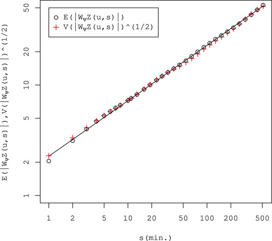
FIGURE 1. Scaling properties of $E\left(\right|W_{\psi }Z[.,s\left(\lambda \right)]\left|\right)$ and $V{\left(\right|W_{\psi }Z[.,s\left(\lambda \right)]\left|\right)}^{1/2}$. The expected value almost perfectly coincides with the standard deviation at all scales. The solid line represents the least-squares fit to the power law function, $2.27s^{0.5}$.

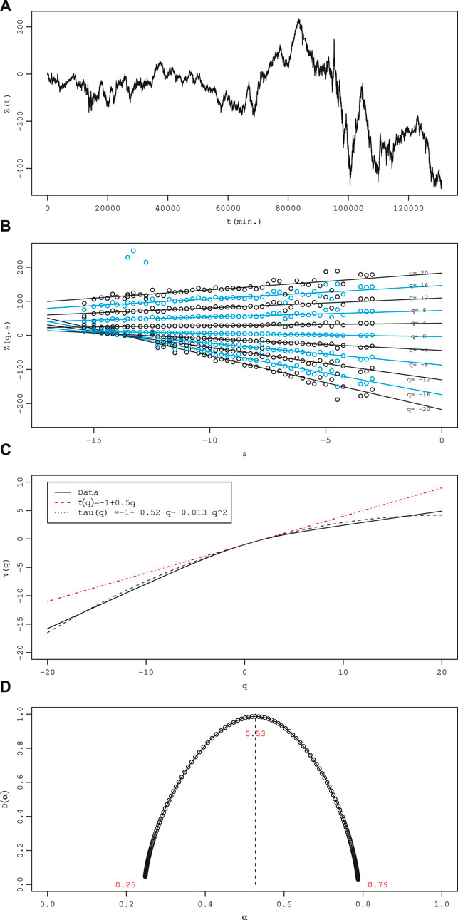
FIGURE 2. Results of multifractal analysis. (A)$Z\left(t\right)$. (B)$Z\left(q,s\right)$ for $q=-20,\dots ,20$ ($\circ$) and regression lines. (C) Scaling exponent $\tau \left(q\right)$ (solid line). The dashed blue line is the least-squares fit to the quadratic function $\tau \left(q\right)=-1+0.52q-0.013q^2$. The dotted red line $\tau \left(q\right)=-1+0.5q$ corresponds to Brownian motion. (D) Singular spectrum $D\left(\alpha \right)$.

The additional additive stochastic process in model Eq. 7 is expected to be a small perturbation to basic model Eq. 4 to avoid violating multifractality. We also impose the following condition for all scales s:

The power law scaling shown in Figure 1,

and condition Eq. 16 show the following constraint condition:

Inserting Eq. 18 into Eq. 15, we also have the equation:

Fokker–Planck Equation

We can derive the Fokker–Planck equation for the stochastic process $\left\{x\left(\lambda \right)\right\}$ expressed by the stochastic differential Eq. 7 as the following [24], which is the master equation that the density of the transition probability $p\left(x,\lambda |x_0,{\lambda }_0\right)$ follows:

Therein, the functions $D_1\left(\lambda ,x\right)$ and $D_2\left(\lambda ,x\right)$ are defined as

The kth moment of the change $\delta x\left(\lambda \right)=x\left(\lambda +\delta \lambda \right)-x\left(\lambda \right)$ induced by the infinitesimal scale transformation $\delta \lambda$ is derived as shown below:

Therein, we used the identity $p\left(y,\lambda |x,\lambda \right)=\delta \left(y-x\right)$. Coefficients $D_1\left(\lambda ,x\right)$ and $D_2\left(\lambda ,x\right)$ show a relation to the first and second moments of $\delta x\left(\lambda \right)$ in the following way:

Coefficients $D_k$ are designated as Kramers–Moyal coefficients [24, 25, 25]. We use Eq. 23 to estimate the function $a_A\left(\lambda \right)$ and $b_A\left(\lambda \right)$ and parameters ${\gamma }_M$ and ${\sigma }_M$. To validate model Eq. 7, it is necessary to confirm vanishing of the kth moments for $3\le k$ in the limit of $\delta \lambda \to 0$. Renner et al. proposed almost identical equations (Eq. 20) within the literature [20, 21], in which they deal with the price change itself as an analogy of the velocity difference in turbulence [19]. They derived a Fokker–Planck equation as a result of their empirical studies using Kramers–Moyal expansion of the Chapman–Kolmogorov equation, regarding the process as a Markovian process.

Empirical Study

Data

We analyze the normalized average of the logarithmic stock prices of the constituent issues of the FTSE 100 Index listed on the London Stock Exchange for November 2007 through January 2009, which includes the Lehman shock of September 15, 2008 and the market crash of October 8, 2008.

Data Processing

First, we calculate the average deseasonalized return of each issue $\delta Z_i\left(t\right)=\text{log}\left(S_i\left(t\right)\right)-\text{log}\left(S_i\left(t-\delta t\right)\right)$, which describes the average change of the portfolio as follows:

where ${\mu }_i$ and ${\sigma }_i$, respectively, denote the average and the standard deviation of $\delta Z_i$ and where $N_F$ represents the number of constituent stock issues (stocks). The constituents of the FTSE 100 Index are updated frequently. We selected $N_F=111$ stocks that remained listed on the London Stock Exchange throughout the period. Here, we set $\delta t=1\min$ and examine the 1-min log return. We excluded the overnight price change and specifically examine the intraday evolutions of returns. To remove the effect of intraday U-shaped patterns of market activity from the time series, the return was divided by the standard deviation of the corresponding time of the day for each issue i. Then, we cumulate $\delta Z\left(t\right)$ to obtain the path of process $Z\left(k\delta t\right) (k=1,\dots ,L)$ (Figure 2A) as follows:

The data size L is $2^{17}$.

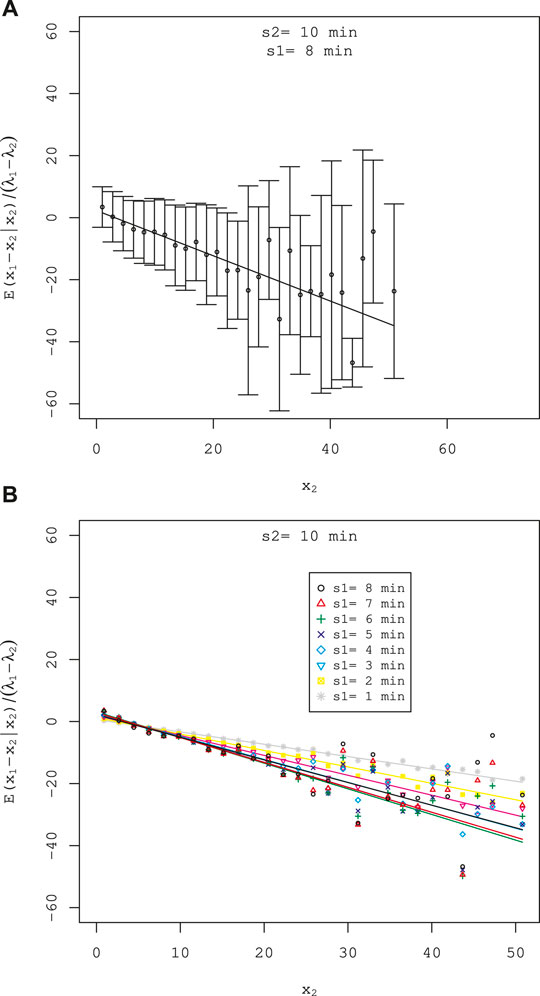
FIGURE 3. Regression of $E(x_1-x_2|x_2=x)/({\lambda }_1-{\lambda }_2)$. (A) The standard errors are denoted by an error bar. (B) Fitting is applied to various $s_1$ and $s_2$ combinations.

Results

Multifractal Analysis

First, we analyze the multifractal properties of the path $Z\left(t\right)$ using an approach with wavelet-based multifractal formalism proposed by Muzy, Bacry, and Arneodo [26, 27, 27]. Initially, we define two mathematical terms. The Hölder exponent $\alpha \left(x_0\right)$ of a function $f\left(x\right)$ at $x_0$ is defined as the largest exponent such that there exist an nth-order polynomial $P_n\left(x\right)$ and constant C that satisfy

where x in a neighborhood of $x_0$, characterizing the regularity of the function $f\left(x\right)$ at $x_0$. The singular spectrum $D\left(\alpha \right)$ is the Hausdorff dimension of the set where the Hölder exponent is equal to α, as follows:

For multifractal paths, the Hölder exponent α is distributed in a range; for paths of the Brownian motion, which are fractal, $D\left(0.5\right)=1$ and $D\left(\alpha \right)=0$ for $\alpha \ne 0.5$.

Muzy, Bacry, and Arneodo proposed the wavelet transform modulus maxima (WTMM) method based on continuous wavelet transform of function to calculate the singular spectrum $D\left(\alpha \right)$. We briefly sketch the WTMM method in Appendix 2. We calculate the partition function $Z\left(q,s\right)$ of the qth moment of wavelet coefficients using Eq. 37 for the path of our data. Results are presented in Figure 2B. The partition function $Z\left(q,s\right)$ for each order q shows power law behavior in the range of scales $s/L<2^{-5}$. Exponents $\tau \left(q\right)$ are derived by Eq. 38. Figure 2C shows that it is a convex function of q. Those results underscore the multifractality of the data path. The singular spectrum $D\left(\alpha \right)$ derived as the Legendre transformation of the function $\tau \left(q\right)$ by Eq. 39 is a convex function that has compact support $\left[0.25,0.79\right]$ taking the peak at $\alpha =0.53$, as shown in Figure 3D.

Parameter Estimations

a_A and γ_M

Parameters $a_A\left(\lambda \right)$ and ${\gamma }_M$ are estimated by taking the limit ${\lambda }_1-{\lambda }_2\to 0$ of the first moment $E\left(x_1-x_2|x_2=x\right)/\left({\lambda }_1-{\lambda }_2\right)\left(\text{LABEL}:\text{K}-\text{M}\right)$. The first moment $E(x_1-x_2|x_2=x)/({\lambda }_1-{\lambda }_2)$ is fitted by a linear function as follows:

where $d\lambda ={\lambda }_1-{\lambda }_2$. As shown in Figure 3A, the first moment is well fitted by a linear function. Fitting of this kind is applied to various ${\lambda }_1=\text{log}\left(L/s1\right)$ and ${\lambda }_2=\text{log}\left(L/s2\right)$ combinations (Figure 3B). Taking the limit $d\lambda \to 0 (ds/s=(s_2-s_1)/s_2\to 0)$, one obtains, $a_A\left({\lambda }_2\right)={\text{lim}}_{d\lambda \to 0}{a}_A\left({\lambda }_2,d\lambda \right)$ ($a_A\left(s_2\right)={\text{lim}}_{ds/s\to 0}{a}_A\left(s_2,ds/s\right)$) and ${\gamma }_M={\text{lim}}_{d\lambda \to 0}{\gamma }_M\left({\lambda }_2,d\lambda \right)$ (${\gamma }_M={\text{lim}}_{ds/s\to 0}{\gamma }_M\left(s_2,ds/s\right)$). Figure 4A presents examples of $a_A\left(s_2,ds/s\right)$ and nonlinear fittings by the function $log\left(a_A\left(s,ds/s\right)\right)=a+b\left(ds/s\right)+c{\left(ds/s\right)}^2$. We estimate $a_A\left(s\right)$ by $a_A\left(s\right)=\text{exp}\left(a\right)$ for each line. The result is presented in Figure 4B. The solid line is the least-squares fit $a_A\left(s\right)$ to a power law function as follows:

where the standard errors are in parentheses. The estimated exponent $0.58\left(0.11\right)$ is consistent with the constraint condition (Eq. 18) within the standard error. By a similar extrapolation $\text{log}\left({\gamma }_M\left(s,ds/s\right)\right)=a+b\left(ds/s\right)+c{\left(ds/s\right)}^2$, we estimate ${\gamma }_M\left(s\right)=exp\left(a\right)$. Figure 5A presents examples of ${\gamma }_M\left(s_2,ds/s\right)$ and nonlinear fittings. We estimate ${\gamma }_M\left(s\right)$ by ${\gamma }_M\left(s\right)=\text{exp}\left(a\right)$ for each line. The result is presented in Figure 5B. We estimate the parameter ${\gamma }_M$ by the average value weighted by the reciprocals of the standard errors as follows:

where the standard error is the value in the parenthesis.

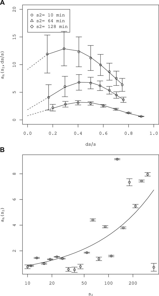
FIGURE 4. Estimation of the parameter $a_A\left(s\right)$. (A) The parameter $a_A\left(s_2,ds/s\right)$ obtained by the regressions shown in Figure 3 and nonlinear fitting $log\left(a_A\left(s,ds/s\right)\right)=a+b\left(ds/s\right)+c{\left(ds/s\right)}^2$. The standard errors of regression Eq. 28 are denoted by an error bar. (B)$a_A\left(s\right)=exp\left(a\right)$ (see the text). The standard errors of nonlinear fittings are denoted by an error bar. The solid line shows the least-squares fit of $a_A\left(s\right)$ to the power law function.

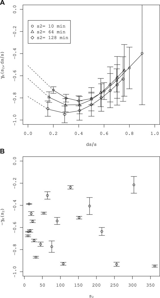
FIGURE 5. Estimation of the parameter ${\gamma }_M$. (A) The parameter ${\gamma }_M\left(s,ds/s\right)$ obtained by the regressions shown in Figure 3 and nonlinear fitting $log\left({\gamma }_M\left(s\right)\right)=a+b\left(ds/s\right)+c{\left(ds/s\right)}^2$. The standard errors of regression Eq. 28 are denoted by an error bar. (B)${\gamma }_M\left(s\right)=exp\left(a\right)$ (see the text). Standard errors of nonlinear fittings are denoted by an error bar.

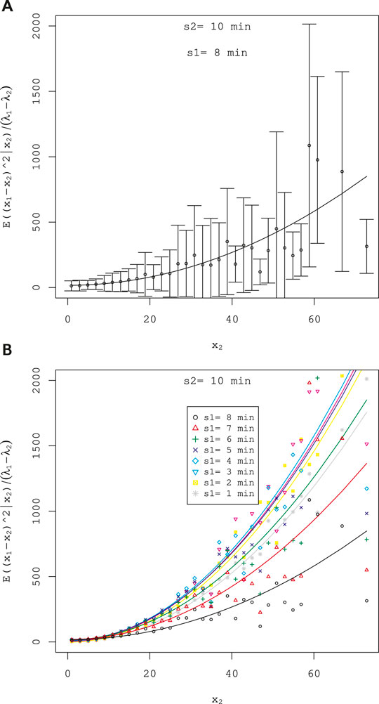
FIGURE 6. Regression of $E\left((x_1-x_2)\right|x_2=x)/({\lambda }_1-{\lambda }_2)$ against $x^2$. (A) Standard errors are denoted by an error bar. (B) Fitting is applied to various $s_1$ and $s_2$ combinations.

b_A and σ_M

Similarly, we estimate parameters $b_A$ and ${\sigma }_M$ by taking the limit ${\lambda }_1-{\lambda }_2\to 0$ of the second moment $E\left({(x_1-x_2)}^2\right|x_2=x)/({\lambda }_1-{\lambda }_2)\left(\text{LABEL}:\text{K}-\text{M}\right)$. The second moment $E\left({(x_1-x_2)}^2\right|x_2=x)/({\lambda }_1-{\lambda }_2)$ is fitted by a quadratic function (a regression against $x^2$) as follows:

As shown in Figure 6A, the second moment is well fitted by a quadratic function. Fitting of this kind is applied to various ${\lambda }_1$ and ${\lambda }_2$ combinations (Figure 6B). Taking the limit $d\lambda \to 0$, one obtains $b_A^2\left({\lambda }_2\right)={\text{lim}}_{d\lambda \to 0}{b}_A^2\left({\lambda }_2,d\lambda \right)$ and ${\sigma }_M^2={\text{lim}}_{d\lambda \to 0}{\sigma }_M^2\left({\lambda }_2,d\lambda \right)$. Figure 7A presents examples of $b_A^2\left(s_2,ds/s\right)$ and nonlinear fitting by the function $log\left(b_A^2\left(s,ds/s\right)\right)=a+b\left(ds/s\right)+c{\left(ds/s\right)}^2$. We estimate $b_A^2\left(s\right)$ for each line by $b_A^2\left(s\right)=\text{exp}\left(a\right)$. The result is presented in Figure 7B. The solid line is the least-squares fit $b_A^2\left(s\right)$ to a power law function as follows:

where the standard errors are in parentheses. The estimated exponent $1.26\left(0.13\right)$ is slightly higher than the constraint condition (Eq 18) $(b_A^2(s)\sim s$). However, it is acceptable with accuracy. By a similar extrapolation $\text{log}\left({\sigma }_M^2\left(s,ds/s\right)\right)=a+b\left(ds/s\right)+c{\left(ds/s\right)}^2$, we estimate ${\sigma }_M^2\left(s\right)=exp\left(a\right)$. Figure 8A presents an example of ${\sigma }_M^2\left(s_2,ds/s\right)$. and an estimate ${\sigma }_M^2\left(s\right)$ by ${\sigma }_M^2\left(s\right)=\text{exp}\left(a\right)$ for each line. The result is shown in Figure 8B. We estimate parameter ${\sigma }_M^2$ by the average value weighted by the reciprocals of the standard errors.

Therein, the standard error is in the parenthesis.

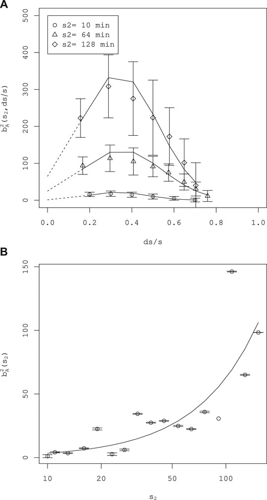
FIGURE 7. Estimation of the parameter $b_A\left(s\right)$. (A) The parameter $b_A\left(s_2,ds/s\right)$ obtained by the regressions shown in Figure 6 and nonlinear fitting $log\left(b_A^2\left(s,ds/s\right)\right)=a+b\left(ds/s\right)+c{\left(ds/s\right)}^2$. The standard errors of the regression Eq. 31 are denoted by an error bar. (B)$b_A^2\left(s\right)=exp\left(a\right)$ (see the text). Standard errors of nonlinear fittings are denoted by an error bar. The solid line shows the least-squares fit of $b_A^2\left(s\right)$ to the power law function.

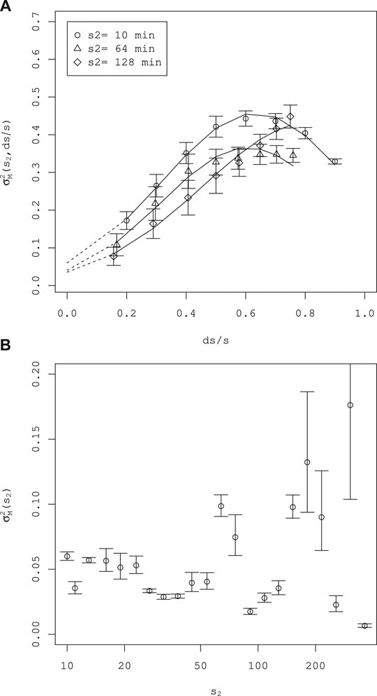
FIGURE 8. Estimation of the parameter ${\sigma }_M$. (A) The parameter ${\sigma }_M\left(s,ds/s\right)$ obtained by the regressions shown in Figure 6 and nonlinear fitting $log\left({\sigma }_M^2\left(s\right)\right)=a+b\left(ds/s\right)+c{\left(ds/s\right)}^2$. The standard errors of regression (Eq. 31 against $x^2$ are denoted by an error bar. (B)${\sigma }_M^2\left(s\right)=exp\left(a\right)$ (see the text). Standard errors of nonlinear fittings are denoted by an error bar.

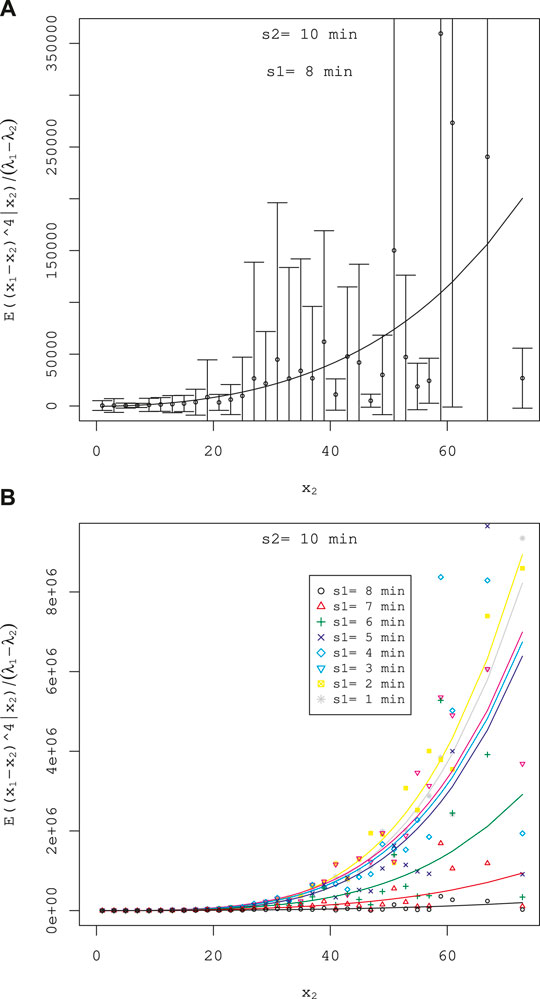
FIGURE 9. Fitting of $E\left({(x_1-x_2)}^4\right|x_2=x)/({\lambda }_1-{\lambda }_2)$ by a quartic function. (A) Standard errors are denoted by the error bar. (B) Fitting is applied to various $s_1$ and $s_2$ combinations.

Higher Moments

Similarly, it is possible to show the kth ($3\le k$) moment $E\left({(x_1-x_2)}^k\right|x_2=x)/({\lambda }_1-{\lambda }_2)$ of the transition probability density $p\left(x_1,{\lambda }_1|{\lambda }_2,x_2\right)$ vanishes in the limit ${\lambda }_1-{\lambda }_2\to 0$. As portrayed in Figure 9A, the fourth moment is well fitted by a quartic function. Applying the fitting to various ${\lambda }_1$ and ${\lambda }_2$ combinations (Figure 9B), we have convinced that the fourth moment vanishes in the limit $d\lambda \to 0$. The Pawula theorem states that all higher Kramers–Moyal coefficients $D_k (3\le k)$ vanish if $D_4$ vanishes [25]. Therefore, we verified Eq 23.

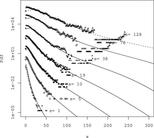
FIGURE 10. Pdf of measured $x\left(\lambda \right)$ and numerical calculation of the Fokker–Planck equation. The result of numerical calculation is represented by the solid lines. Marks are measured values. The scale is attached to each line.

Numerical Calculation of the Fokker–Planck Equation

We confirmed that estimation of the parameter $a_A\left(\lambda \right)$ and $b_A\left(\lambda \right)$ by the $E\left({\left(x_1-x_2\right)}^k|x_2=x/\left({\lambda }_1-{\lambda }_2 \right)\right)\left(k=\mathrm{1,2}\right)$ is consistent with the constraint condition (Eq. 18) with accuracy. If one imposes the other constraint (Eq. 19, then the parameters take the following functional form:

where ϵ is a small parameter. The consistent range of ϵ found by estimation of Eq 29 and Eq 32 is $0.15\le \mathit{ϵ}\le 0.34$. To fix parameters ${\gamma }_M$ and ${\sigma }_M$, we use the empirical value of the scaling exponent $\tau \left(q\right)$, which is fitted by the quadratic function $\tau \left(q\right)=-1+0.52q-0.013q^2$ (see Figure 2C). One can derive $\tau \left(q\right)=-1+\left({\gamma }_M+\frac{1}{2}{\sigma }_M^2\right)q-\frac{1}{2}{\sigma }_M^2{q}^2$ for the basic model (Eq. 4 without additional stochastic processes. Again using the assumption of slight perturbation, then from the coefficients of the quadratic function, the parameters ${\gamma }_M$ and ${\sigma }_M$ are expected to exist respectively in the neighborhood of ${\gamma }_M=0.51$ and ${\sigma }_M=0.026$. Next, we try the value of the parameters ${\gamma }_M=0.51$, ${\sigma }_M=0.026$, and $\mathit{ϵ}=0.16$ for numerical calculation of the Fokker–Planck equation. Results are presented in Figure 10. The initial pdf of the numerical calculation represented by the dashed line was based on the measured pdf on scale $s=128\left(min\right)$. In the initial values, the fine fluctuation was smoothed using a spline function with the rationale that small fluctuations in the measured pdf are attributable to the finiteness of the number of observations. The tails are extrapolated using a power function with index $-4.9$ which is obtained empirically. For time evolution, the fourth-order explicit Runge–Kutta method was used. The solid line is the calculation result obtained using the estimated value of the parameters ${\gamma }_M=0.51$, ${\sigma }_M=0.026$, and $\mathit{ϵ}=0.16$. The dotted line is the result obtained when $\mathit{ϵ}=0$. The difference between the two was very small. The results closely matched the actual pdf. In the data and the numerical calculation, the probability density function does not converge to zero at the origin because of the finite size of the bin. Although the details around the origin $x=0$ cannot be empirically discussed due to the finiteness of the observed data, the probability density function must converge to zero at the origin if the negative qth moment of the fluctuation is requested to converge.

Using results of the numerical calculation of the pdf obtained at each scale, we calculate the scaling exponent $\tau \left(q\right)$ as shown follows:

The result is presented in Figure 11. No difference exists between the two numerical calculation results. Both curves are convex upward, indicating multifractal properties. Comparison with measured values is also good. These results, when combined with consideration of the statistics of multipliers given in 2.1.2, underscore the effectiveness of the continuous cascade model Eq. 7 with additive stochastic processes proposed.

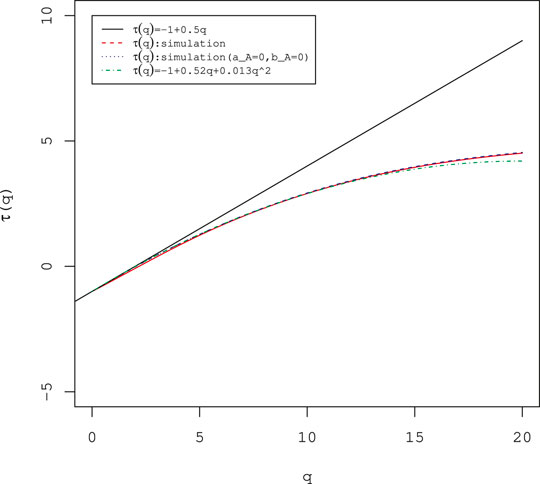
FIGURE 11. Scaling exponent $\tau \left(q\right)$. A representation of each line is shown in the legend.

Discussion

The random cascade model has evolved as a model of developed turbulence. The original model, in which the stochastic process that connects each layer of the spatial scale is an independent random multiplication process, contradicts results obtained through empirical research. Therefore, an improved discrete random multiplicative cascade model with additional additive stochastic processes was proposed along with a model formulated as a Fokker–Planck equation by considering cascade processes as a continuous Markov process. Moreover, those models have been applied to data analysis of the stock market and the foreign exchange market, where they have been successful. Herein, we propose a continuous cascade model formulated as a stochastic differential equation of volatility including two independent modes of Brownian motion: one has multiplicative coupling with volatility; the other has additive coupling, as in an improved discrete cascade model for the stock market, with effectiveness clarified by results of earlier research [18]. The model parameters were estimated by application to a stock price time series. The Fokker–Planck equation was derived from the stochastic differential equation as a master equation with the transition probability density function of volatility. Furthermore, the model parameters were estimated by its application to the average stock price time series made from FTSE 100 constituents listed on the London Stock Exchange. At that time, as an alternative variable of volatility, the wavelet transform coefficient with the second derivative of the Gaussian function as an analyzing wavelet was used. Numerical calculation of the Fokker–Planck equation was conducted using the estimated parameter values. The results reported herein faithfully reproduce the results of an earlier empirical study. This model includes information about neither the time axis nor the sign of the price fluctuation, which is necessary for a model of price fluctuations. The actual stock market exhibits well-known properties that break symmetry with respect to the time axis, such as the causal structure from long-term to short-term scale volatility described first in Introduction and price–volatility correlation (leverage effect) [412]. Therefore, the extension of the random cascade model to encompass these phenomena remains as a subject for future work.

Data Availability Statement

Publicly available datasets were analyzed in this study. This data can be found here: Historic Price Service (HPS) provided by the London Stock Exchange (https://www.londonstockexchange.com/products-and-services/reference-data/hps/hps.htm).

Author Contributions

JM conducted the empirical and numerical study of the model based on the dataset. KK theoretically analyzed the model. All authors agree to be accountable for the contents of the work.

Funding

This research was partially supported by a Grant-in-Aid for Scientific Research (C) No. 16K01259.

Conflict of Interest

The authors declare that the research was conducted in the absence of any commercial or financial relation that could be construed as a potential conflict of interest.

Acknowledgments

One author, JM, expresses special appreciation for support by a Seijo University Special Research Grant.

Appendix 1

Derivation of Eq 15

We introduce some notation for simplification of the description:

From Eq. 13, we have

We also have

Because of the coincidence of the expected value and the standard deviation, we have $E_2(\lambda )=2E_1^2(\lambda )$ and $E_2(\lambda +d\lambda )=2E_1^2(\lambda +d\lambda )$. Inserting those equalities and using approximation $e^{{\sigma }_M^{2}d\lambda }=1$, we have the constraint condition 15.

Appendix 2

WTMM Method

The WTMM method builds a partition function from the modulus maxima of the wavelet transform defined at each scale s as the local maxima of $\left|W_{\psi }\left[f\right](x,s)\right|$ regarded as a function of x. Those maxima mutually connect across scales and form ridge lines designated as maxima lines. The set $\mathrm{ℒ}(s_0)$ is the set of all the maxima lines l which satisfy

The partition function is defined by the maxima lines as

Assuming power law behavior of the partition function

one can define the exponents $\tau (q)$. The singular spectrum $D(\alpha )$ can be computed using the Legendre transform of $\tau (q)$:

References

1. Müller UA, Dacorogna MM, Davé RD, Olsen RB, Pictet OV, von Weizsäcker JE. Volatilities of different time resolutions–analyzing the dynamics of market components. J Empir Finance. (1997). 4:213–39. doi:10.1016/s0927-5398(97)00007-8.
2. Arnéodo A, Muzy J-F, Sornette D. “Direct” causal cascade in the stock market. Eur Phys J B. (1998). 2:277–82. doi:10.1007/s100510050250.
3. Lynch PE, Zumbach GO. Market heterogeneities and the causal structure of volatility. Quant Finance. (2003). 3:320–31. doi:10.1088/1469-7688/3/4/308.
4. Cont R. Empirical properties of asset returns: stylized facts and statistical issues. Quant Finance. (2001). 1:223–36. doi:10.1080/713665670.
5. Richardson LF. Weather prediction by numerical process. Cambridge UK: Cambridge University Press (1922). p. 236.
6. Kolmogorov AN. The local structure of turbulence in incompressible viscous fluids for very large Reynolds numbers. Dokl Akad Nauk SSSR. (1941). 30:301–5.
7. Kolmogorov AN. A refinement of previous hypotheses related to the local structure of turbulence in a viscous incompressible fluid at high Reynolds number. J Fluid Mech. (1962). 13:301–5. doi:10.1017/s0022112062000518.
8. Mandelbrot BB. Intermittent turbulence in self-similar cascades: divergence of high moments and dimension of the carrier. J Fluid Mech. (1974). 62:331–58. doi:10.1017/s0022112074000711.
9. Frisch U. Turbulence: the legacy of A. Kolmogorov. Cambridge, UK: Cambridge University Press (1997). p. 312.
10. Ghashghaie S, Breymann W, Peinke J, Talkner P, Dodge Y. Turbulent cascades in foreign exchange markets. Nature. (1996). 381:767–70. doi:10.1038/381767a0.
11. Schmitt F, Schertzer D, Lovejoy S. Multifractal analysis of foreign exchange data. Appl Stoch Model Data Anal. (1999). 15:29–53. | doi:10.1002/(sici)1099-0747(199903)15:1<29::aid-asm357>3.0.co;2-z.
12. Bouchaud J-P, Potter M. Theory of financial risk and derivative pricing: from statistical physics to risk management. 2nd ed. Cambridge, UK: Cambridge University Press (2003). p. 400.
13. Arneodo A, Bacry E, Muzy JF. Random cascades on wavelet dyadic trees. J Math Phys. (1998). 39:4142–64. doi:10.1063/1.532489.
14. Breymann W, Ghashghaie S, Talkner P. A stochastic cascade model for Fx dynamics. Int J Theor Appl Finance. (2000). 03:357–60. doi:10.1142/s021902490000019x.
15. Chen Q, Chen S, Eyink GL. Kolmogorov’s third hypothesis and turbulent sign statistics. Phys Rev Lett. (2003). 90:254501. doi:10.1103/physrevlett.90.254501. |
16. Jiménez J. Intermittency and cascades. J Fluid Mech. (2000). 409:99–120. doi:10.1017/s0022112099007739.
17. Jiménez J. Intermittency in turbulence. Proceedings of the 15th “Aha Huliko” a Winter Workshop, 2007 January 23–26; Honolulu,Publication Services, SOEST, University of Hawaii; (2007). p. 99–120.
18. Maskawa J-i., Kuroda K, Murai J. Multiplicative random cascades with additional stochastic process in financial markets. Evol Inst Econ Rev. (2018). 15:515–29. doi:10.1007/s40844-018-0112-y.
19. Friedrich R, Peinke J. Description of a turbulent cascade by a Fokker-Planck equation. Phys Rev Lett. (1997). 78:863–6. doi:10.1103/physrevlett.78.863.
20. Renner C, Peinke J, Friedrich R. Evidence of Markov properties of high frequency exchange rate data. Phys Stat Mech Appl. (2001). 298:499–520. doi:10.1016/s0378-4371(01)00269-2.
21. Renner C, Peinke J, Friedrich R. Experimental indications for Markov properties of small-scale turbulence. J Fluid Mech. (2001). 433:383–409. doi:10.1017/s0022112001003597.
22. Siefert M, Peinke J. Complete multiplier statistics explained by stochastic cascade processes. Phys Lett. (2007). 371:34–8. doi:10.1016/j.physleta.2007.05.111.
23. Reinke N, Fuchs A, Nickelsen D, Peinke J. On universal features of the turbulent cascade in terms of non-equilibrium thermodynamics. J Fluid Mech. (2018). 848:117–53. doi:10.1017/jfm.2018.360.
24. Peinke C. Stochastic methods. 4th ed. Berlin Heidelberg, Germany: Springer-Verlag (2009). p. 447.
25. Risken H. The fokker–planck equation. 2nd ed. Berlin Heidelberg, Germany: Springer-Verlag (1889). p. 472.
26. Muzy JF, Bacry E, Arneodo A. Multifractal formalism for fractal signals: the structure-function approach versus the wavelet-transform modulus-maxima method. Phys Rev E. (1993). 47:875–84. doi:10.1103/physreve.47.875.
Keywords: Fokker–Planck equation, intermittency, Langevin equation, Markovian process, multifractal
Citation: Maskawa J-i and Kuroda K (2020) Model of Continuous Random Cascade Processes in Financial Markets. Front. Phys. 8:565372. doi: 10.3389/fphy.2020.565372
Received: 25 May 2020; Accepted: 29 October 2020;
Published: 27 November 2020.
Edited by:
Wei-Xing Zhou, East China University of Science and Technology, ChinaReviewed by:
Haroldo V. Ribeiro, State University of Maringá, BrazilJoachim Peinke, University of Oldenburg, Germany
Copyright © 2020 Maskawa and Kuroda. This is an open-access article distributed under the terms of the Creative Commons Attribution License (CC BY). The use, distribution or reproduction in other forums is permitted, provided the original author(s) and the copyright owner(s) are credited and that the original publication in this journal is cited, in accordance with accepted academic practice. No use, distribution or reproduction is permitted which does not comply with these terms.
*Correspondence: Jun-ichi Maskawa, maskawa@seijo.ac.jp