Exploring the Trophic Spectrum: Placing Mixoplankton Into Marine Protist Communities of the Southern North Sea

1. Introduction

Plankton communities form the base of all open-water ecosystems. Traditionally, organisms of these communities have been primarily classified into either phototrophs or heterotrophs. However, the dichotomous plankton classification has been increasingly questioned, and now the photo-phago mixotrophic potential (i.e., the combination of photo- and phagotrophy in one cell) of many phytoplankton and protozooplankton species is being recognized (Flynn et al., 2013; Glibert, 2016; Mitra et al., 2016; Stoecker et al., 2017). Flynn et al. (2019) proposed to use the term mixoplankton for these organisms and the terms phyto- or protozooplankton, respectively, for organisms incapable of phagotrophy or phototrophy.

Mixoplankton have the potential to access more resources than are available to pure phyto- and protozooplankton (Barton et al., 2013; Stoecker et al., 2017). By employing both photo- and phagotrophy, mixoplankton can overcome the limitations of low inorganic nutrient environments that restrict the growth of phytoplankton or prey limitations that restrict the growth of protozooplankton. Mitra et al. (2016) provided a functional classification separating mixoplankton into different groups. Constitutive Mixoplankton (CM) have the innate ability to perform photosynthesis while Non-Constitutive Mixoplankton (NCM) need to acquire photosynthetic capabilities from their prey. As a result, the different types of mixoplankton have varying abiotic and biotic requirements (Anschütz and Flynn, 2020).

Mixoplankton can potentially increase the trophic transfer efficiency (Stoecker et al., 2017). Including mixoplankton in aquatic ecosystem models is necessary to capture this change in system dynamics (Mitra et al., 2014; Ghyoot et al., 2017; Flynn et al., 2018). Furthermore, mixoplankton are important for the management of marine environments, as many harmful algal bloom species are known mixoplankton (e.g., Dinophysis) (Burkholder et al., 2008; Reguera et al., 2012). For modeling and management discussions, it is important to research the trophic composition of plankton communities and link the trophic composition to abiotic environments.

The link between marine phytoplankton communities and abiotic environments has long been researched. The Southern North Sea microplankton community has also been well-studied; Baretta-Bekker et al. (2009) and Prins et al. (2012) did so using data from the same monitoring program employed in this study. Most of these studies did not include the role of mixoplankton. However, there have been various local (e.g., Stoecker et al., 1989; Löder et al., 2012; Duhamel et al., 2019) and even specific global (Harrison et al., 2011) studies of certain mixoplankton groups. More recently, Leles et al. (2017, 2019) and Faure et al. (2019) presented the first comprehensive analyses on the global biogeography of mixoplankton. While Hansson et al. (2019) recently published a study on abiotic drivers of mixoplankton in boreal lakes, our work is, to the best of our knowledge, the first study that addresses the relation between marine plankton community assessments in different abiotic environments and the identification of potential mixoplankton in these marine communities.

However, even when a consensus to include mixoplankton in ecosystem studies is reached, a high uncertainty remains when assigning a trophic mode to taxa. Many chlorophyll-containing flagellates are classified as phototrophs by default while most are actually potentially mixotrophic (Selosse et al., 2017). The difficulty of observing marine mixoplankton feeding in the wild or in the laboratory adds to this uncertainty (Worden et al., 2015; Anderson et al., 2017; Stoecker et al., 2017).

Currently, there are two contrasting views on the trophic mode of marine plankton communities present in literature. On the one hand, photo- or phagotrophy are assumed to be the default trophic modes of all planktonic protists. If photo-phago-mixotrophy is considered at all, only taxa proven to be capable of such are classified as mixoplankton. On the other hand, if photo-phago-mixotrophy is assumed to be the default trophic mode in all protists, then only taxa proven to be incapable of photo-phago-mixotrophy are classified as phyto- or protozooplankton (Flynn et al., 2013; Mitra et al., 2014; Leles et al., 2017, 2019).

The aim of this study is to explore the uncertainty of these two trophic views and their implications for plankton community assessments using quantitative, long term data. To do this, we exploited a 24 year-long time series on abiotic and protist data in the Southern North Sea along with literature on mixoplankton. While most routine monitoring data on protists fail to count small and fragile protists (Haraguchi et al., 2018; Flynn et al., 2019), routine monitoring data such as the ones employed in this study are still useful as they cover a long time frame and a wide range of abiotic gradients. This makes the dataset ideal for researching the trophic composition of protist communities in varying abiotic environments.

Using this dataset, we studied three trophic classifications to take the trophic uncertainty of marine protist communities into account. In classification A (the “documented mixoplankton” classification), only documented mixoplankton were labeled as such. In classification B (the “presumed mixoplankton” classification), only diatoms, cyanobacteria, and colonial Phaeocystis were labeled as phytoplankton. The other motile, phototrophic taxa and documented mixoplankton were labeled as mixoplankton. Then, using a principle component analysis (PCA), we constructed a third numerical classification (classification C – the “environmentally-defined mixoplankton” classification) in which documented mixoplankton and motile, phototrophic taxa associated with documented mixoplankton were labeled as mixoplankton. Due to the trophic uncertainty, we were not able to verify the results of the different classifications against other existing datasets. Thus, we proceeded to use literature and a partial redundancy analysis (RDA) to determine which classification seemed the most likely.

More specifically, the steps taken in this study were (1) to determine the spatial and temporal variations of the abiotic parameters and the protist communities, (2) to establish where mixoplankton occur in the Southern North Sea, (3) to determine which abiotic factors favor mixoplankton, and (4) to explore the implications of the three trophic classifications.

2. Materials and Methods

2.1. Study Site

The North Sea is a shallow marginal sea of the Atlantic Ocean located on the European continental shelf. The North Sea is roughly divided into two regions, the Northern and the Southern North Sea. This study focuses on the Dutch continental shelf in the Southern North Sea (51–55 °N) (see Figure 1).

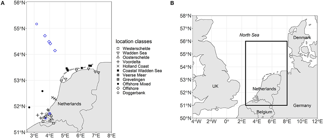
Figure 1. (A) The map displays the locations of the 37 sampling stations in the Southern North Sea labeled according to their location class. Black indicates that only surface samples were taken. Blue indicates that summer stratification occurred and three depths were sampled (surface, pycnocline, and bottom). (B) The map places the sampling region within the context of the North Sea.

In terms of inorganic nutrients, the Southern North Sea ranges from nutrient-rich estuaries to offshore regions that seasonally become relatively nutrient-poor (van Beusekom and Diel-Christiansen, 2009). The Southern North Sea is also highly diverse in terms of stratification and seasonality. Where tidal currents dominate, continuous vertical mixing of the water column occurs. Regions of freshwater influence are (often intermittently) salinity stratified, while deeper waters with less tidal influence show intermittent or seasonal thermal stratification (Große et al., 2016). Apart from nutrient and stratification gradients, the Southern North Sea is also impacted by gradients of suspended sediments, dissolved oxygen, pH, and salinity (Emeis et al., 2015).

The Southern North Sea is an umbrella term for regions commonly referred to as the Southern Bight, the Wadden Sea and the Doggerbank (Beets and van der Spek, 2000). The depth of the Southern Bight and the Wadden Sea increases from the coast toward the central North Sea. The central North Sea can reach down to 40 m depth. However, the Doggerbank, which is located in the central North Sea, is only 18 m deep (Nielsen et al., 1993). Based on these hydrographic environments and geographic locations, we grouped 37 stations into 11 location classes (see Figure 1).

The Westerschelde, the Wadden Sea, and the Oosterschelde are geographically distinct environments. The location class Voordelta groups coastal sampling stations northwest of the Rhine estuary. The location class Holland Coast groups sampling stations northeast of the Rhine estuary that lie in the region of freshwater influence (Simpson et al., 1993). The sampling stations north of the Wadden Sea barrier islands were grouped into the location class Coastal Wadden Sea. The Veerse Meer was separated from the North Sea and the Oosterschelde in 1961 and reopened toward the Oosterschelde in 2004. Thus, the Veerse Meer has a unique hydrographic environment (Bakker, 1972). Grevelingen is a closed-off arm of the Rhine-Meuse estuary with a sluice maintaining the saline character of the system. The location class Offshore Mixed had no records of summer stratification over the 24 year period and was thus separated from the Offshore location class. Doggerbank was placed into a separate location class due to its shallow depth.

2.2. Datasets

In our study, we used abiotic and protist data from 1990 to 2014 that were sampled by the Rijkswaterstaat monitoring program (RWS– Dutch Directorate-General for Public Works and Water Management). On average, the 37 stations were monitored every four weeks from October to February and every 2 weeks from March to September. The abiotic and protist samples were usually taken at the same time. However, after 2010, the sampling frequency of plankton data decreased and from 2010 onward, for all stations (with the exception of Doggerbank), protist samples were taken quarterly during the growth season (March–September). Doggerbank was sampled once in each of the months January, April, June, and August. The samples were taken at the surface (typically at 1 m depth). When stations showed (seasonal) stratification, they were sampled near the bottom and pycnocline as well. In this study, we focused on the routine sampling data for surface-waters; in doing so it should be noted that seasonal mixing of the water column affects how well such sampling reflects the whole protist community. To determine the yearly vs. spatial variation in the datasets, we conducted an estimation of variance components analysis (VCA) using the R-package VCA (Schuetzenmeister and Dufey, 2019) (see Supplementary Data Sheet for more details).

2.2.1. Abiotic Data

The abiotic data were retrieved from a Deltares database (Waterbase Deltares, 2019). Nutrients, i.e., $\text{N}{\text{O}}_3^{-}$, $\text{N}{\text{H}}_4^{+}$, NO₂, dissolved inorganic phosphate (DIP) measured as soluble reactive phosphate, dissolved inorganic silica (DISi), total nitrogen (TN; the sum of dissolved inorganic, dissolved organic, and particulate organic nitrogen), as well as suspended sediment and salinity were extracted. Dissolved inorganic nitrogen (DIN) was calculated from its separate components (DIN = $\text{N}{\text{O}}_3^{-}+\text{N}{\text{H}}_4^{+}+\text{N}{\text{O}}_2$). The data were grouped according to the previously described location classes. For DIP, outliers (values over the 98th percentile) were removed.

In addition, the relative availability of DIN was determined using the ratio of organically bound nitrogen (orgN) to total nitrogen $\left(\frac{\text{orgN}}{\text{TN}}=\frac{\text{TN}-\text{DIN}}{\text{TN}}\right)$. Margalef (1963) defined maturity in terms of energy flow. Applying this line of thought, we termed this ratio the index of ecosystem maturity (IEM) as it describes the shift from abundant inorganic to mostly organism-bound nitrogen typical for ecosystem maturation. Thus, the IEM enables a comparison between environmental systems that differ from each other in terms of absolute nitrogen concentrations. The IEM is given as a value between 1 (mature) and 0 (immature).

2.2.2. Protist Data

The protist data were retrieved from the RWS data servicedesk (RWS, 2019). The dataset contains information on taxa, location, cell counts, biovolumes, biomass as well as trophic mode. During monitoring, 1 L plankton bottle samples were collected and preserved with 4 mL acid Lugol's iodine. The samples were then identified and counted using inverted microscopy to determine the number of cells per taxon. As the sampling technique was not optimized toward sampling ciliates, ciliates (with the exception of Mesodinium rubrum) were not counted. Whenever possible, the cells were identified down to their species level, otherwise the cells were identified to their genus or higher taxonomic levels. Cell counts were transformed into carbon biomass using biovolume coefficients (Baretta-Bekker et al., 2009). The sampling methodologies can be reviewed in more detail in Baretta-Bekker et al. (2009) and Prins et al. (2012). The taxa were matched against the World Register of Marine Species (WoRMS Editorial Board, 2019) and the accepted scientific name was used for the subsequent analysis to harmonize taxonomic names over the 24 year time period.

A partial PCA as well as a partial RDA was completed using the vegan package in R (Stevens et al., 2019). We used the partial PCA to determine the environmental envelope of proven mixoplankton. We define an environmental envelope as the polygon that encloses all taxa of a certain group, in this case the proven mixoplankton. We used the partial RDA to associate the different trophic groups with the abiotic factors. Due to changes in the identification and counting protocol in 2000 and the change of sampling frequencies after 2010, an observer effect was applied as a condition within the partial PCA and RDA, which ensures that the resulting axes are linearly unrelated to the observer effect.

For each classification, the fraction of each trophic mode of the total biomass per month, year, and location class was calculated. The trophic mode was processed in three different ways to study the three trophic classifications. Supplementary Table 1 provides a summary of all three trophic classifications.

2.2.2.1. Classification A: documented mixoplankton

Literature by Jeong et al. (2010), Löder et al. (2012), Leles et al. (2017), and Leles et al. (2019) was used to identify taxa with a documented ability to perform photo-phago mixotrophy. These taxa were binned as “mixoplankton” and the type of mixotrophy as per Mitra et al. (2016) was allocated. The other taxa were binned as “phytoplankton” or “protozooplankton.” When a taxon was only identified down to genus level and species belonging to that genus were also present in the dataset, the entire genus was assigned the trophic mode that was most abundant (in terms of biomass) among the species belonging to that genus. Five taxa (class Dinophyceae, family Gymnodiniaceae, family Peridiniaceae, order Peridiniales, class Raphidophyceae) were labeled as “unknown trophy” as it was not possible to assign a trophic mode to those taxonomic ranks with confidence.

2.2.2.2. Classification B: presumed mixoplankton

According to the functional classification argued by Flynn et al. (2013), Mitra et al. (2016) and Flynn et al. (2019), all organisms capable of phototrophy were labeled as “mixoplankton” except for those that are proven to be incapable of phagocytosis. Thus, only diatoms, cyanobacteria and colonial Phaeocystis were labeled as “phytoplankton”. The “protozooplankton” remained the same as in classification A.

2.2.2.3. Classification C: environmentally-defined mixoplankton

Proven mixoplankton and motile, phototrophic taxa associated with the environmental envelope of proven mixoplankton were binned as “mixoplankton”. Phototrophic taxa not associated with the environmental envelope of proven mixoplankton as well as diatoms, cyanobacteria and colonial Phaeocystis were labeled as “phytoplankton”. The “protozooplankton” remained the same as in the other two classifications.

3. Results

3.1. Abiotic Data

Figures 2 and 3 visualize the nutrient concentrations (DIN, DIP, and DISi) and the IEM as well as suspended sediment, salinity and stratification for each location class. In all figures, abiotic gradients from the estuaries to the offshore are evident. Based on these abiotic parameters, the location classes can be grouped into four systems.

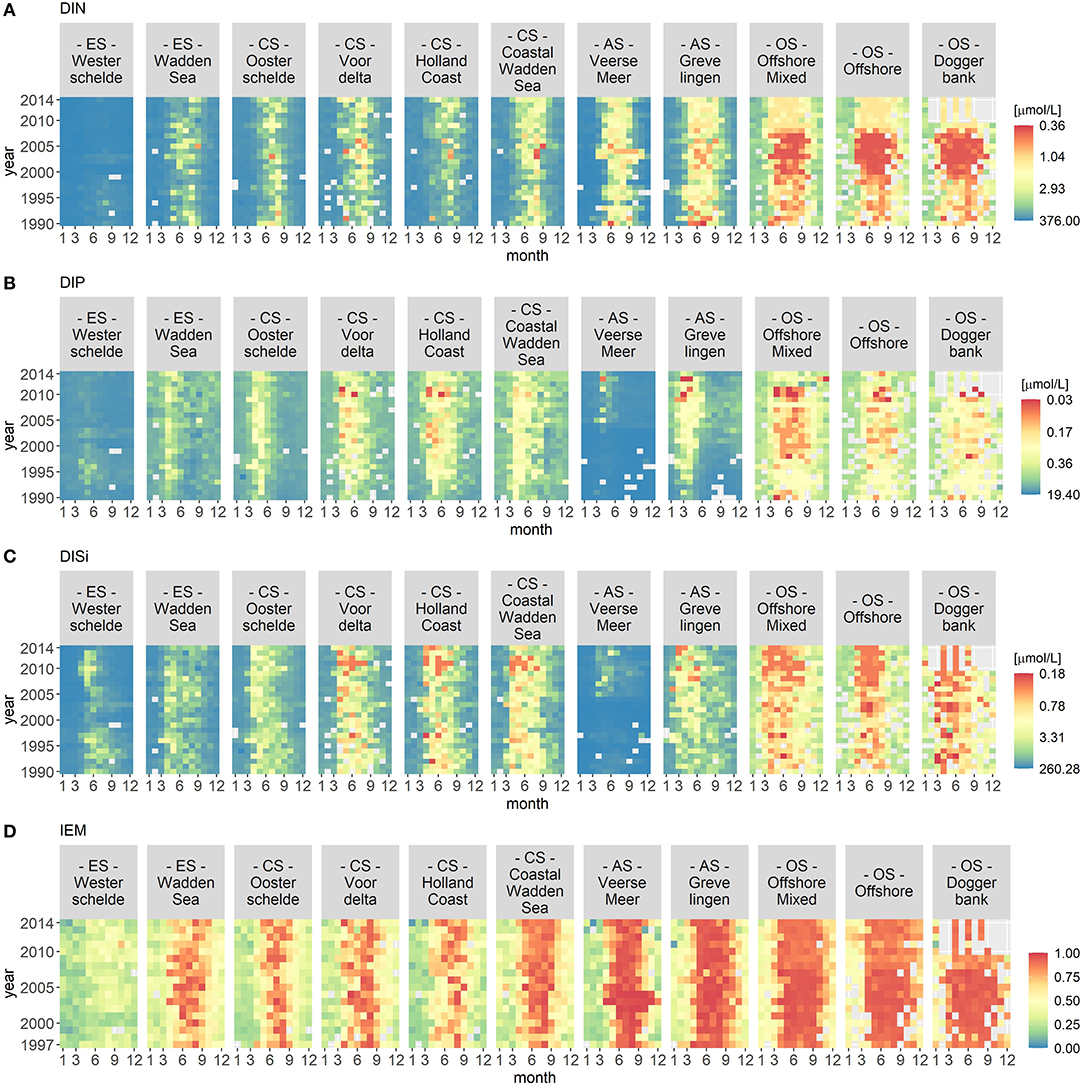
Figure 2. Monthly median of nutrient concentrations for DIN (A), DIP (B), and DISi (C) as well as the IEM (index of ecosystem maturity – D) for each location class per year. The nutrient concentrations were hyperbolically transformed. The location classes are grouped into estuary (ES), coastal (CS), anthropogenically modified (AS), and offshore systems (OS). The figures display gradients (left to right) from the estuary systems (ES) to the offshore systems (OS).

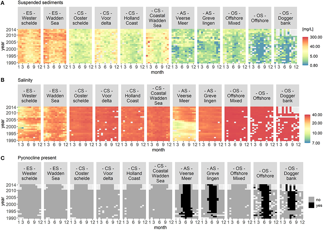
Figure 3. Monthly median of suspended sediments (A), salinity (B), and stratification (C) for each location class per year. Suspended sediment and salinity use a logarithmic color scale. The location classes are grouped into estuary (ES), coastal (CS), anthropogenically modified (AS), and offshore systems (OS). The figures display gradients (left to right) from the estuary systems (ES) to the offshore systems (OS). In (C), the color black indicates that a pycnocline was detected at the location classes Veerse Meer, Grevelingen, Offshore, and Doggerbank.

(1) Unstratified estuary systems (ES): Westerschelde and Wadden Sea. Both location classes were characterized by salinity values around 20 and high suspended sediment values (long term average of 50 mg/L). The Westerschelde had a low IEM and high DIN, DIP, and DISi concentrations throughout the time period with the exception of DISi that showed a slight decrease during summer. During summer, the Waddensea had a high IEM and medium DIN, DIP, and DISi concentrations.

(2) Unstratified coastal systems (CS): Oosterschelde, Voordelta, Holland Coast, and Coastal Wadden Sea. These location classes could be clearly separated from the other location classes by their salinity (around 30) and their suspended sediment values (between 20 and 45 mg/L). Compared to the estuary systems, the coastal systems had lower nutrient concentrations during summer. After 2010, the DISi concentration decreased. All four location classes showed seasonality in the IEM (high during summer).

(3) Seasonally stratified, anthropogenically modified systems (AS): Veerse Meer and Grevelingen. Both location classes were characterized by low salinity and suspended sediment values. Both location classes had low DIN concentrations and had a high IEM during summer. While Grevelingen displayed decreased DIP and DISi concentrations during spring, Veerse Meer had high nutrient concentrations throughout this time period. The opening of the Veerse Meer to the Oosterschelde in 2004 was reflected in the salinity and suspended sediment values.

(4) Offshore systems (OS): Offshore Mixed (unstratified), Offshore (stratified), and Doggerbank (stratified). These location classes were characterized by high salinity (35) and very low suspended sediment values. The offshore systems had very low nutrient concentrations during summer and had high IEM. Compared to the coastal systems (category 2), the period nutrient concentration decrease was longer in the offshore systems. The DIN concentrations decreased from 2000 to 2006, while the DISi concentrations decreased after 2007.

Year-to-year variations were visible for all location classes, especially for Veerse Meer. However, the VCA showed that the location classes contributed over 80% of the variation while the yearly changes contributed <4%.

3.2. Protist Data

The protist data set contained 621 unique taxa in a size range from 1 to 800 μm. It should be noted that small nanoflagellates might be poorly represented (see Supplementary Figure S1). Table 1 summarizes the number of taxa per trophic mode for each classification and Table 2 summarizes the trophic modes of the five most abundant taxonomic classes.

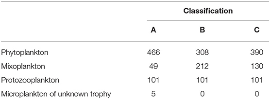
Table 1. Number of taxa per trophic mode and trophic classification.

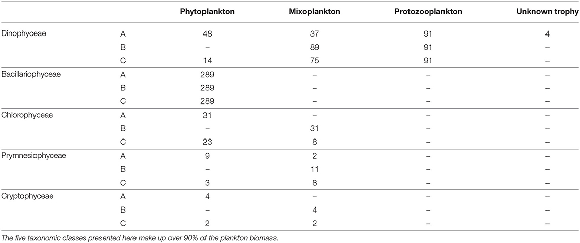
Table 2. Types of trophic mode for the five most important taxonomic classes for each trophic classification.

Figure 4 visualizes the site ordination plots from the partial PCA of the protist data. The ordination plot is dominated by two gradients. In Figure 4A, the estuaries compose a group in the upper right quadrant, the coastal systems are grouped around the origin while the anthropogenically modified and offshore systems are grouped toward the lower left quadrant. Thus, the location class gradient divides the ordination plot into two triangles with a top right triangle depicting the estuaries and a bottom left triangle depicting the offshore systems. No distinguishable trend from year to year can be seen in Figure 4B. Figure 4C shows a clear seasonal pattern with the seasons gradient dividing the ordination plot into two triangles—a top left triangle depicting the fall/winter months and a bottom right triangle depicting the spring/summer months.

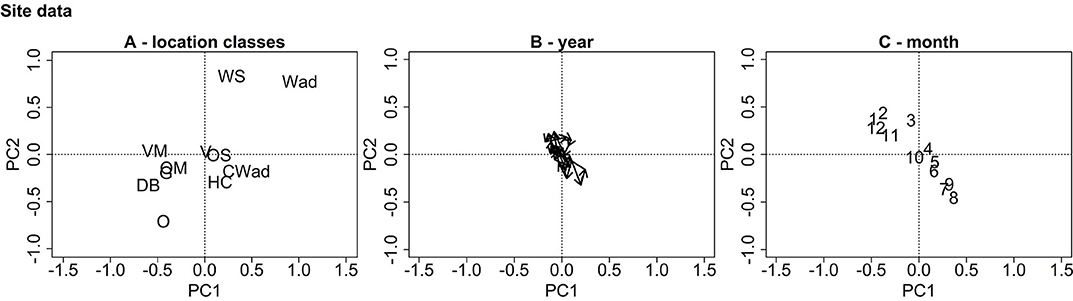
Figure 4. PCA ordination plots for the site data. Subfigure (A) displays the ordination centers for the location classes (WS, Westerschelde; Wad, Wadden Sea; OS, Oosterschelde; VD, Voordelta; HC, Holland Coast; CWad, Coastal Wadden Sea; VM, Veerse Meer; G, Grevelingen; OM, offshore mixed; O, Offshore; D, Doggerbank), (B) the ordination centers for the years and (C) the ordination centers for the months. The plots are dominated by two opposite, diagonally oriented gradients representing the location classes and months.

Figure 5 display the species scores from the partial PCA for all three trophic classifications and they highlight the differences in the mixoplankton between the three different trophic classifications. All protists are located in the spring/summer months triangle which corresponds to the protists growth period.

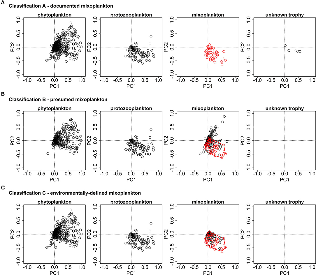
Figure 5. PCA ordination plots for the species data of the three trophic classifications. (A) The documented mixoplankton (in red) are oriented toward the bottom right quadrant. (B) The presumed mixoplankton are oriented toward both right quadrants. The documented mixoplankton of (A) are displayed in red and the red polygon highlights the environmental envelope of the documented mixoplankton. (C) The documented mixoplankton are displayed in red and the additional environmentally-defined mixoplankton are displayed in black. The additional environmentally-defined mixoplankton were chosen as they lie within the environmental envelope of documented mixoplankton of (A) (displayed by the red polygon).

For classification A, the protozooplankton, mixoplankton, and microplankton of unknown trophy occupy the lower right quadrant (corresponding to the summer months and non-estuary systems), while the phytoplankton extend over both right quadrants (corresponding to the summer months and all location classes). For classification B, mixoplankton form two groups one in the lower right quadrant (corresponding to the summer months and non-estuary systems) and one in the upper right quadrant (corresponding to the summer months and the estuary system). The orientation of phytoplankton and protozooplankton is the same as in trophic classification A. For classification C, only those motile, phototrophic taxa of classification B that were located within the environmental envelope of proven mixoplankton were retained in the mixoplankton category and so the orientation of mixoplankton for classification C corresponds to that of classification A. Supplementary Table 2 provides a list of motile, phototrophic taxa associated with the environmental envelope of proven mixoplankton.

3.2.1. Trophic Classification A (Documented Mixoplankton)

Trophic classification A visualizes the trophic composition of the protist community in which only proven mixoplankton were classified as such. Figure 6A displays the biomass per month, year and location class for each trophic mode. The fraction of mixoplankton displayed a clear spatial gradient and was highest in the offshore location classes. Figure 6B shows that the mixoplankton consisted almost entirely of CMs.

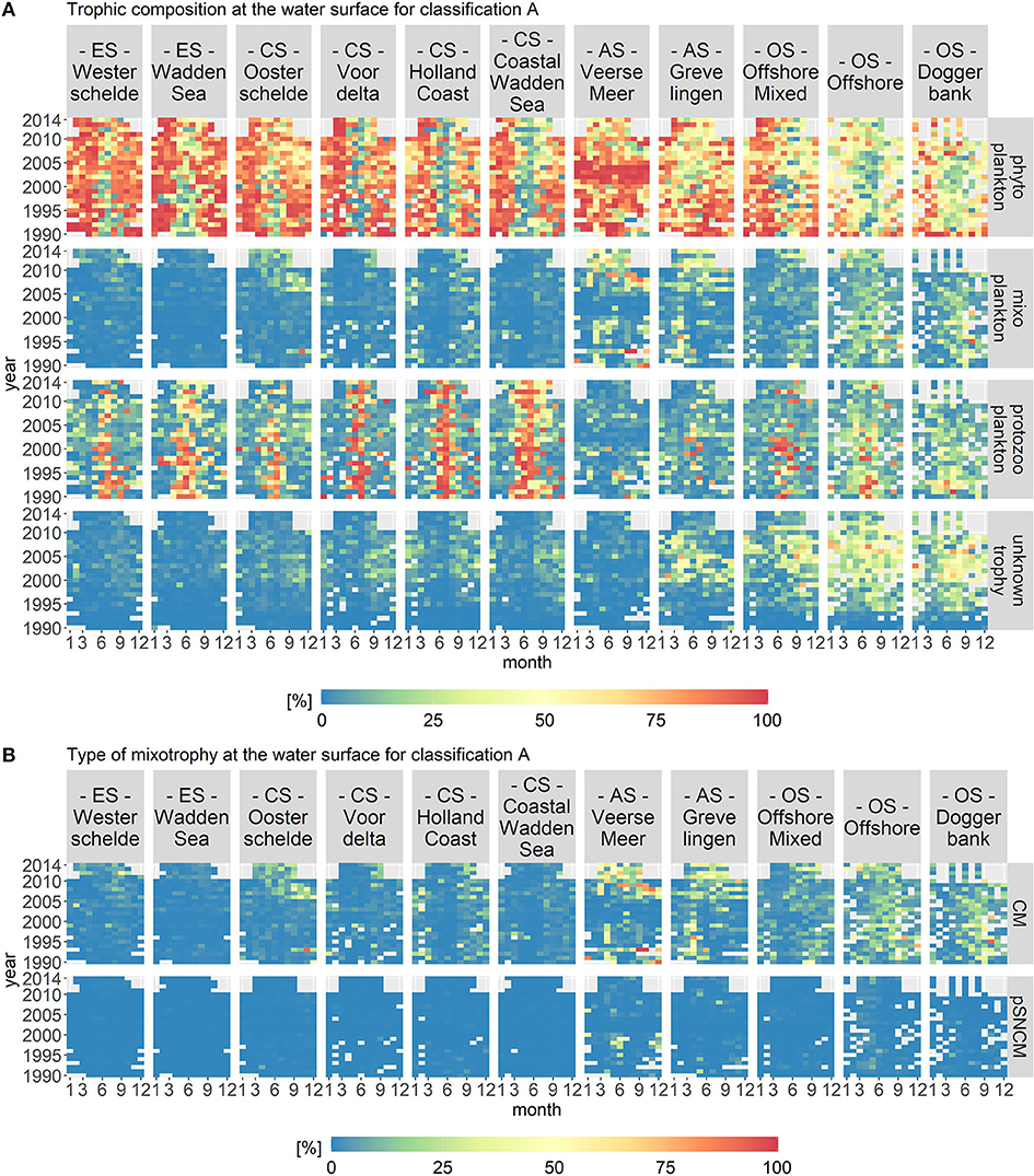
Figure 6. Monthly fractions of the total biomass per trophic mode (A) and per type of mixotrophy (B) for trophic classification A. The location classes are grouped into estuary (ES), coastal (CS), anthropogenically modified (AS), and offshore systems (OS). CM stands for Constitutive Mixoplankton and pSNCM for plastid Specialist Non-Constitutive Mixoplankton, which are a subcategory of NCMs. The occurrence of CMs displays a clear spatial gradient.

In the estuary systems (Westerschelde and Wadden Sea), phytoplankton constituted the largest part of the plankton community in April/May as well as in August/September. Protozooplankton constituted the largest group in June or July, depending on the year. In the estuaries, mixoplankton and microplankton of unknown trophy did not contribute notably to the overall plankton composition.

In the coastal systems (Oosterschelde, Voordelta, Holland Coast, and Coastal Wadden Sea), phytoplankton were the largest group in April/May as well as in August/September, whereas protozooplankton were the largest group in June/July. In the Coastal Wadden Sea, protozooplankton constituted the largest group into early autumn. In the four coastal systems, microplankton of unknown trophy contributed around 25% to the protist community during August and September. For all coastal systems, mixoplankton contributed only slightly to the trophic plankton composition during the late summer/fall period. However, after 2009 in the Oosterschelde, mixoplankton contributed around 25% to the protist community during summer and fall.

The anthropogenically modified systems (Veerse Meer and Grevelingen) differed from the estuary and coastal systems through their lack of a consistent protozooplankton bloom in the summers. For both location classes, mixoplankton peaked during a few months over the 24 year time period to over 50% of the community biomass. In Veerse Meer, phytoplankton were the largest group throughout the whole period. However, in Grevelingen, phytoplankton did not dominate to the same extent. Microplankton of unknown trophy contributed notably to Grevelingen, which was not the case for Veerse Meer.

The offshore systems (Offshore Mixed, Offshore, and Doggerbank) displayed a diverse trophic composition. For these location classes, phytoplankton constituted the largest group in spring. The rest of the year, microplankton of unknown trophy made up around 50% and mixoplankton 25% of the plankton community. There was no consistent fraction of protozooplankton during the summer months.

The temporal variations in the plankton data were more pronounced compared to the abiotic data. However, the VCA showed that the spatial components contributed more to the variation (over 25%) than the temporal components (<10%). The temporal variations visible in the abiotic data for the anthropogenically modified systems were not visible in the plankton data.

3.2.2. Trophic Classification B (Presumed Mixoplankton)

Figure 7 displays the biomass per month, year and location class for each trophic mode for trophic classification B. In contrast to classification A, classification B assumed all motile, phototrophic taxa to be mixoplankton. Only diatoms, cyanobacteria, and colonial Phaeocystis are classified as phytoplankton. The protozooplankton remained the same as in classification A. The fraction of mixoplankton was highest in the offshore location classes and mixoplankton seasonally occurred in the early summer and fall at all location classes.

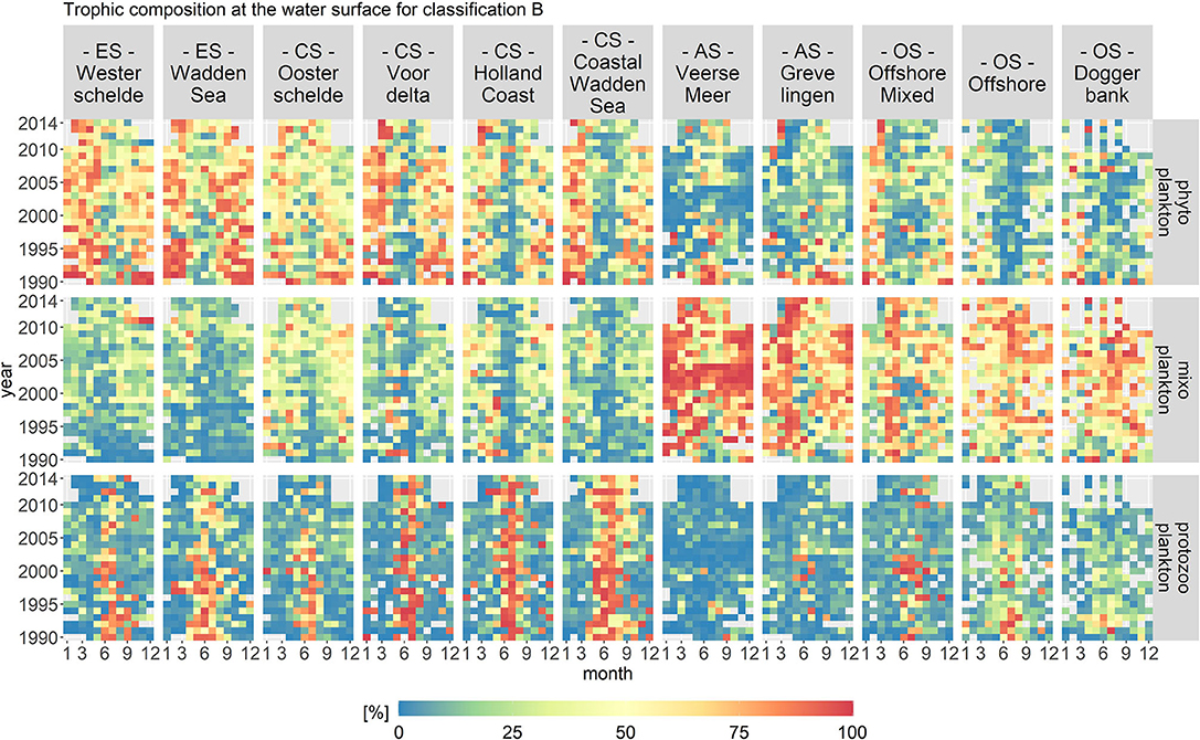
Figure 7. Monthly fractions of the total biomass per trophic mode for trophic classification B. The location classes are grouped into estuary (ES), coastal (CS), anthropogenically modified (AS), and offshore systems (OS). The fraction of mixoplankton is highest in the offshore location class. All location classes display a seasonal occurrence of mixoplankton in the early summer and fall.

The spatial distribution for classification B remained, in principle, the same as for classification A. The highest fraction of mixoplankton still occurred in the offshore and anthropologically modified location classes. However, the seasonal succession of trophic modes changed as compared to trophic classification A. The mixoplankton fraction increased at all location classes in the early summer and fall compared to classification A. The anthropogenically modified systems displayed interesting anomalies. From 2002 to 2004 in Veerse Meer, mixoplankton (taxa Chlorophyceae) contributed around 100% to the protist community. During the summer months after 2006, phytoplankton and mixoplankton both contributed equally (both 50%) to the plankton community. Overall, Grevelingen had a high fraction of mixoplankton in the early spring season.

The temporal variations in classification B were more pronounced as compared to classification A. Nonetheless, the VCA showed that the spatial components contributed more to the variation (over 50%) than the temporal components (10%). The temporal variations visible in the abiotic data for the anthropogenically modified systems were reflected in classification B.

3.2.3. Trophic Classification C (Environmentally-Defined Mixoplankton)

Figure 8 displays the biomass per month, year and location class for each trophic mode for trophic classification C. Classification C categorized mixoplankton using the partial PCA results. For classification C only documented mixoplankton and motile, phototrophic taxa associated with the environmental envelope of documented mixoplankton were labeled as mixoplankton. In contrast to the other two trophic classifications, the seasonal distribution of mixoplankton for all location classes was oriented more toward the late summer/autumn season.

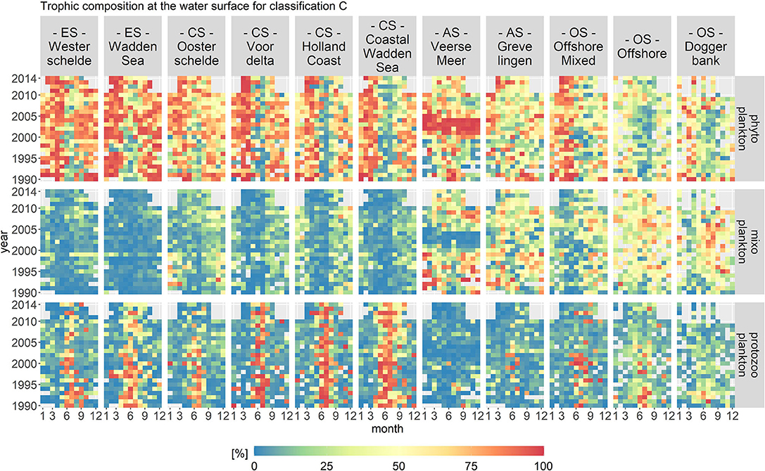
Figure 8. Monthly fractions of the total biomass per trophic mode for trophic classification C. The location classes are grouped into estuary (ES), coastal (CS), anthropogenically modified (AS), and offshore systems (OS). The mixoplankton fraction displays a clear spatial and seasonal gradient.

The mixoplankton fraction displayed a clear spatial and seasonal gradient. Spatially, the mixoplankton fraction was highest in the offshore location classes. Seasonally, mixoplankton occurred more during the late summer months. Especially in the estuary and coastal location classes, a seasonal succession of trophic modes was visible from phyto- (spring) to protozoo- (summer) to mixoplankton (fall). Veerse Meer and Grevelingen were exceptions. In Grevelingen, mixoplankton contributed 50% to the plankton community during the whole year. Veerse Meer displayed a stark shift from 2002 to 2004 in which phytoplankton completely dominated the plankton community (taxa Chlorophyceae). This shift coincided well with the opening of Veerse Meer to the Oosterschelde.

Of all three trophic classifications, the temporal variations in classification C were the most pronounced, which was especially visible in the trophic composition of Veerse Meer. However, the temporal contribution to variance was still small (around 10%) compared to the spatial contribution (over 40%).

3.3. Abiotic Drivers of Mixoplankton Distribution

Figure 9 displays the partial RDA ordination plots for phytoplankton and mixoplankton for the three trophic classifications. For all three trophic classifications of Figure 9A, phytoplankton are oriented toward the suspended sediment gradient. In Figure 9B, documented and environmentally-defined mixoplankton (trophic classifications A and C) are oriented toward the IEM and nutrient concentration gradients and away from the suspended sediment gradient. The assumption that all motile, phototrophic protist are mixoplankton (as in trophic classification B) places some mixoplankton along the suspended sediment gradient, which is clearly associated with phytoplankton (see Figure 9A).

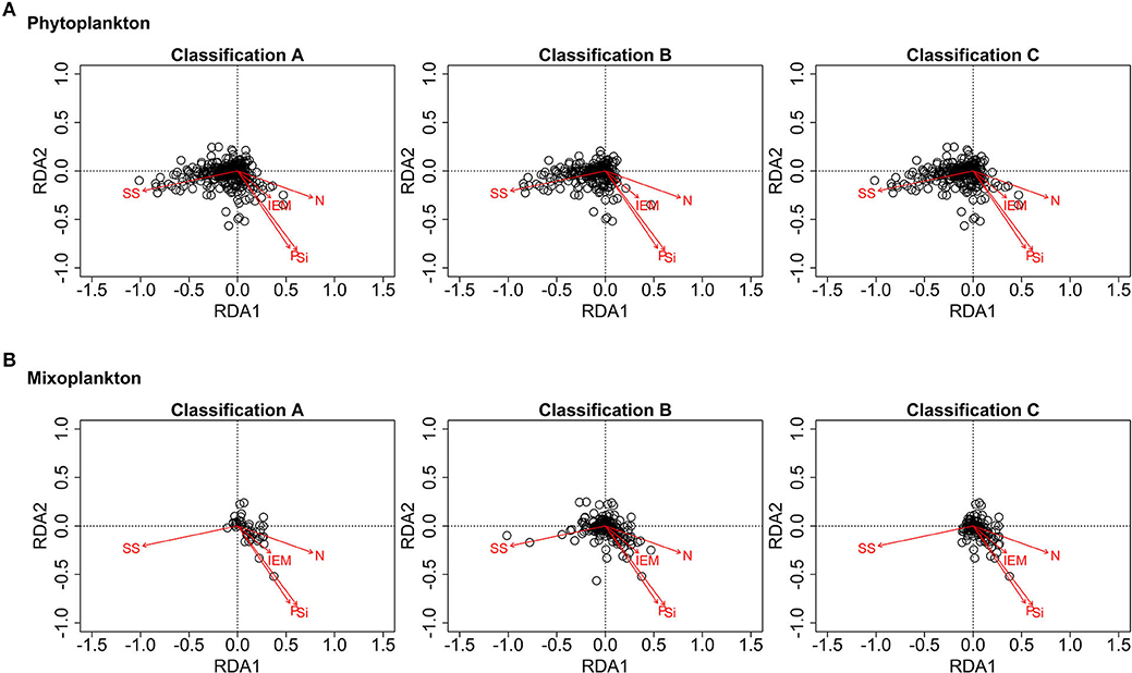
Figure 9. RDA ordination plots for phytoplankton (A) and mixoplankton (B) (SS, suspended sediment; IEM, index of ecosystem maturity; N/P/Si, nitrogen, phosphorus, silica concentration). (A) Phytoplankton are oriented along the suspended sediment gradient. (B) Documented and likely mixoplankton are oriented toward the IEM and nutrient concentration gradients.

4. Discussion

By exploring three trophic classifications, this study helps close a gap between plankton community assessments within varying abiotic environments and our developing knowledge of mixoplankton. It makes use of a dataset that covers a wide range of taxa, a long time period and strong abiotic gradients. We did not discover any basin-wide yearly trends in the trophic composition of the protist community. This is consistent with the absence of basin-wide yearly trends in abiotic parameters as the North Sea system is mainly driven through large scale hydrodynamics and terrestrial runoff (Emeis et al., 2015).

Peperzak (2010) showed an observer effect linked to changes in the identification and counting protocols in 2000. As the sampling frequency after 2010 changed as well, we took both changes into account by employing a partial PCA and RDA. However, we did not take these observer effects into account in the trophic aggregation for the heatmaps. Apart from an apparent increase of mixoplankton in Oosterschelde after 2009, the trophic classifications do not display other changes that can be linked to the observer effects. The reason for this lies in the aggregation of the protist data at the trophic level. The trophic level is directly related to the abiotic system though inorganic nutrients, light and food availability. The apparent increase of mixoplankton in Oosterschelde was caused by the identification of the mixoplankton Micromonas sp., which before 2009 was grouped into the phytoplankton classes Chlorophyceae or Prasinophyceae (Brochard et al., 2013). We conclude that by aggregating on a trophic level, the timeseries becomes independent of the observer effects and is thus suitable for analyzing the trophic composition of protist communities.

Furthermore, in the offshore environments, the sampling frequency declined after 2010. While Hinder et al. (2012) found a marked increase in the ratio of diatoms to dinoflagellates after 2006 using data from the continuous plankton recorder, we could not determine such a marked increase in our dataset. The dataset used in our study is decidedly different from continuous plankton recorder datasets and more suited to the analysis of mixoplankton because of the observed size range (Flynn et al., 2019). However, especially for Doggerbank, the bloom succession becomes indistinguishable due to the low sampling intervals.

In order to determine the contribution of mixoplankton to the trophic composition of plankton communities, we studied three trophic classifications. We determined that in inorganic nutrient-depleted, seasonally stratified, predominantly offshore environments, mixoplankton periodically constitute up to 25% (classification A – documented mixoplankton), over 75% (classification B – proven mixoplankton), or around 50% (classification C – environmentally-defined mixoplankton) of the protist community. An oligotrophic environment is clearly associated with mixoplankton (Troost et al., 2005; Hartmann et al., 2012; Stoecker and Lavrentyev, 2018; Duhamel et al., 2019; Livanou et al., 2019). However, comparing the determined percentages with current literature is more difficult. Mixoplankton contribution to a certain community is often either sampled within a certain size fraction (Safi and Hall, 1999; Anderson et al., 2017; Sato et al., 2017), within certain taxa (Li et al., 2000; Millette et al., 2017; Haraguchi et al., 2018) or with a certain grazing focus (Unrein et al., 2007).

In general, the sampled size range coincides well with the size range in which mixoplankton occur (Flynn et al., 2019). However, nanoflagellates were most likely undersampled and ciliates other than M. rubrum were not counted. This is in general an issue for most (routine) monitoring programs (Haraguchi et al., 2018). Many nanoflagellates can be mixotrophic (Safi and Hall, 1999) and some ciliates are NCMs as they can retain kleptochloroplastids (Haraguchi et al., 2018). Stelfox-Widdicombe et al. (2004) showed that in offshore environments, ciliates constitute 50% of the microzooplankton community and of those ciliates, 50% are mixotrophic. In nearshore environments, heterotrophic dinoflagellates dominate the microzooplankton community and oligotrich ciliates contribute around 20% to the microzooplankton community. Thus, it can be said that the trophic composition of the studied community in reality includes more protozoo- and mixoplankton. While CMs are known to belong to the most abundant types of mixoplankton (Faure et al., 2019), the lack of ciliates and the low abundance of Dinophysis (NCMs) is also the reason for the dominance of CMs in the Southern North Sea.

While all trophic classifications clearly associate mixoplankton with certain location classes, the trophic classifications differ in terms of mixoplankton seasonality and succession. Classifications A and C display a clear seasonal succession of trophic modes as described in Mitra et al. (2014). In classification B, which presumes all phototrophic organisms to be capable of mixotrophy unless they have been explicitly proven incapable, mixoplankton additionally occur in the estuaries during winter/early spring, in which there is low light, high turbidity and an ample amount of inorganic nutrients. While Millette et al. (2017) showed that in the Choptank river (U.S.A.) Heterocapsa rotundata employs mixotrophy to overcome light limitation in winter, the nutrient concentrations in that study were much lower as compared to the nutrient concentrations of the Westerschelde and the Wadden Sea. There is little evidence of mixoplankton in turbid, eutrophic, temperate systems (such as the Southern North Sea estuaries).

We conclude that classifications A (documented mixoplankton) and B (presumed mixoplankton) display the two extremes of the trophic spectrum. While classification A is still highly subjected to the traditional dichotomy, classification B places mixoplankton into improbable environments. Clearly, the actual trophic composition of protist communities in the Southern North Sea lies in between trophic classifications A and B. Classification C (environmentally-defined mixoplankton) provides an indication of what the actual trophic composition could possibly look like. Classification C classifies mixoplankton according to environmental conditions associated with proven mixoplankton. Furthermore, classification C does not pre-define mixoplankton to certain broad functional groups as trophic classification B does. Using the partial PCA scores, we can provide a list of likely unrecognized mixoplankton in the Southern North Sea (see Supplementary Table 2). Many of these taxa belong to the class Dinophyceae as well as the phyla Haptophyta and Chlorophyta which are associated with mixoplankton (Stoecker and Lavrentyev, 2018).

The offshore environments of the Southern North Sea in which we predominantly found mixoplankton are generally characterized by a low total biomass and thus mixoplankton do not necessarily contribute notably to the absolute biomass of the Southern North Sea. However, as certain cryptic mixoplankton are often associated with noxious or harmful events (Davidson et al., 2014), properly accounting for changes in trophic plankton composition is nonetheless important. Furthermore, Bouvier et al. (1997) found that even though mixoplankton biomass is often significantly lower than those of other trophic modes, their high specific ingestion rates let mixoplankton contribute significantly to the grazing of bacteria and nanoplankton, indicating a local importance.

In inorganic nutrient depleted, seasonally stratified, low biomass environments, mixoplankton have a clear advantage over phyto- and protozooplankton as they can use their mixotrophic capabilities to obtain nutrients and energy from multiple sources. In inorganic nutrient replete, turbid environments such as the estuary systems, phytoplankton are at an advantage due to their superior light-harvesting capabilities (Geider et al., 1997). This explains the strong orientation of phytoplankton along the suspended sediment gradient in the RDA (see Figure 9). In environments with abundant prey, protozooplankton are at an advantage due to their superior prey ingestion capabilities in the dark (Skovgaard, 1996; Li et al., 1999; Adolf et al., 2006; Anderson et al., 2018).

The environments in which mixoplankton occur are often called mature (Mitra et al., 2014; Flynn et al., 2018; Haraguchi et al., 2018). In many studies, maturity is often associated with geographic location and/or season. This study proposes the IEM (index of ecosystem maturity) as a functional definition of energy flow based on measured environmental parameters. It describes the shift from abundant inorganic to mostly organism-bound nitrogen typical for ecosystem maturation. Consequently, the IEM provides information on the availability of inorganic nutrients without being pre-defined to occur at a particular location or season. We conclude from the partial RDA results that our proposed IEM along with low turbidity provides an indication on the relevance of mixoplankton in plankton communities.

In the coming years, with advancements of laboratory and field methods along with the new understanding of mixoplankton, the trophic composition of plankton communities can be refined. This study demonstrates that numerical ecology methods can assist experimental methods in the attempt to determine mixoplankton in plankton communities. Yet, it remains difficult to determine the cause and effect between abiotic and plankton systems using only field data. Modeling provides a tool (Flynn and Mitra, 2009) to test hypotheses on the causal relationship between abiotic environments and the trophic composition of plankton communities. Until now, mixotrophy as a functional trait is still poorly represented in aquatic ecosystem models (Ghyoot et al., 2017). Including mixotrophy into aquatic ecosystem models changes the overall allocation of nutrient and energy resources within the base of marine ecosystems. Furthermore, by including mixotrophy into aquatic ecosystem models, hypotheses on the trophic spectrum could be tested.

Plankton communities are the base of our marine ecosystems. With climate change (Hays et al., 2005) and offshore wind farms (Heath et al., 2017) changing the marine coastal environment, we need to better understand the trophic composition of plankton communities within their abiotic environment (Caron, 2016). This study provides a first quantitative delineation of the possible boundaries of the trophic spectrum within marine protist communities and provides a list of potential unrecognized mixoplankton in the Southern North Sea. It can serve as a benchmark for subsequent efforts to include mixotrophy into ecosystem models as well as placing mixoplankton into marine plankton community assessments.

Data Availability Statement

Publicly available datasets were analyzed in this study. This data can be found at: https://www.emodnet-biology.eu/; https://opendap.deltares.nl.

Author Contributions

LS undertook the primary data analysis and preparation of the figures, building from ideas generated by all the authors as well as anonymous reviewers. LS drafted the manuscript. All authors contributed to the development of the subsequent manuscript revisions.

Funding

This project has received funding from the European Union's Horizon 2020 research and innovation programme under the Marie Skłodowska-Curie grant agreement No 766327 (project MixITiN).

Conflict of Interest

The authors declare that the research was conducted in the absence of any commercial or financial relationships that could be construed as a potential conflict of interest.

Acknowledgments

The authors want to thank three reviewers to a previous version of this work for their comments which greatly helped improve this manuscript.

Supplementary Material

The Supplementary Material for this article can be found online at: https://www.frontiersin.org/articles/10.3389/fmars.2020.586915/full#supplementary-material

References

Adolf, J. E., Stoecker, D. K., and Harding, L. W. (2006). The balance of autotrophy and heterotrophy during mixotrophic growth of Karlodinium micrum (Dinophyceae). J. Plankton Res. 28, 737–751. doi: 10.1093/plankt/fbl007
Anderson, R., Charvet, S., and Hansen, P. J. (2018). Mixotrophy in chlorophytes and haptophytes-effect of irradiance, macronutrient, micronutrient and vitamin limitation. Front. Microbiol. 9:1704. doi: 10.3389/fmicb.2018.01704
Anderson, R., Jürgens, K., and Hansen, P. J. (2017). Mixotrophic phytoflagellate bacterivory field measurements strongly biased by standard approaches: a case study. Front. Microbiol. 8:1398. doi: 10.3389/fmicb.2017.01398
Anschütz, A., and Flynn, K. (2020). Niche separation between different functional types of mixoplankton: results from NPZ-style N-based model simulations. Mar. Biol. 167:3. doi: 10.1007/s00227-019-3612-3
Bakker, C. (1972). Milieu en plankton van het Veerse Meer, een tien jaar oud brakwatermeer in Zuidwest-Nederland. Hydrobiol. Veren. 6, 15–38. doi: 10.1007/BF02336207
Baretta-Bekker, J. G., Baretta, J. W., Latuhihin, M. J., Desmit, X., and Prins, T. C. (2009). Description of the long-term (1991-2005) temporal and spatial d1istribution of phytoplankton carbon biomass in the Dutch North Sea. J. Sea Res. 61, 50–59. doi: 10.1016/j.seares.2008.10.007
Barton, A. D., Pershing, A. J., Litchman, E., Record, N. R., Edwards, K. F., Finkel, Z. V., et al. (2013). The biogeography of marine plankton traits. Ecol. Lett. 16, 522–534. doi: 10.1111/ele.12063
Beets, D. J., and van der Spek, A. J. (2000). The Holocene evolution of the barrier and the back-barrier basins of Belgium and the Netherlands as a function of late Weichselian morphology, relative sea-level rise and sediment supply. Geol. Mijnbouw Netherl. J. Geosci. 79, 3–16. doi: 10.1017/S0016774600021533
Bouvier, T., Becquevort, S., and Lancelot, C. (1997). Biomass and feeding activity of phagotrophic mixotrophs in the northwestern Black Sea during the summer 1995. Hydrobiologia 363, 289–301. doi: 10.1023/A:1003196932229
Brochard, C., van den Oever, A., van Wezel, R., Koeman, R., Koeman, T., and Mulderij, G. (2013). Geannoteerde Soortenlijst Biomonitoring Fytoplankton Nederlandse Zoete Wateren 1990-2012. Technical report, Koeman en Bijkerk bv, Haren.
Burkholder, J. A. M., Glibert, P. M., and Skelton, H. M. (2008). Mixotrophy, a major mode of nutrition for harmful algal species in eutrophic waters. Harmful Algae 8, 77–93. doi: 10.1016/j.hal.2008.08.010
Caron, D. A. (2016). Mixotrophy stirs up our understanding of marine food webs. Proc. Natl. Acad. Sci. U.S.A. 113, 2806–2808. doi: 10.1073/pnas.1600718113
Davidson, K., Gowen, R. J., Harrison, P. J., Fleming, L. E., Hoagland, P., and Moschonas, G. (2014). Anthropogenic nutrients and harmful algae in coastal waters. J. Environ. Manage. 146, 206–216. doi: 10.1016/j.jenvman.2014.07.002
Duhamel, S., Kim, E., Sprung, B., and Anderson, O. R. (2019). Small pigmented eukaryotes play a major role in carbon cycling in the P-depleted western subtropical North Atlantic, which may be supported by mixotrophy. Limnol. Oceanogr. 64, 2424–2440. doi: 10.1002/lno.11193
Emeis, K. C., van Beusekom, J., Callies, U., Ebinghaus, R., Kannen, A., Kraus, G., et al. (2015). The North Sea - A shelf sea in the Anthropocene. J. Mar. Syst. 141, 18–33. doi: 10.1016/j.jmarsys.2014.03.012
Faure, E., Not, F., Benoiston, A. S., Labadie, K., Bittner, L., and Ayata, S. D. (2019). Mixotrophic protists display contrasted biogeographies in the global ocean. ISME J. 13, 1072–1083. doi: 10.1038/s41396-018-0340-5
Flynn, K. J., and Mitra, A. (2009). Building the “perfect beast”: modelling mixotrophic plankton. J. Plankton Res. 31, 965–992. doi: 10.1093/plankt/fbp044
Flynn, K. J., Mitra, A., Anestis, K., Anschütz, A. A., Calbet, A., Ferreira, G. D., et al. (2019). Mixotrophic protists and a new paradigm for marine ecology: where does plankton research go now? J. Plankton Res. 41, 375–391. doi: 10.1093/plankt/fbz026
Flynn, K. J., Mitra, A., Glibert, P. M., and Burkholder, J. M. (2018). “Mixotrophy in harmful algal blooms: by whom, on whom, when, why, and what next,” in Global Ecology and Oceanography of Harmful Algal Blooms. Ecological Studies (Analysis and Synthesis), Vol. 232, eds P. Glibert, E. Berdalet, M. Burford, G. Pitcher, and M. Zhou (Cham: Springer). doi: 10.1007/978-3-319-70069-4_7
Flynn, K. J., Stoecker, D. K., Mitra, A., Raven, J. A., Glibert, P. M., Hansen, P. J., et al. (2013). Misuse of the phytoplankton-zooplankton dichotomy: the need to assign organisms as mixotrophs within plankton functional types. J. Plankton Res. 35, 3–11. doi: 10.1093/plankt/fbs062
Geider, R. J., MacIntyre, H. L., and Kana, T. M. (1997). Dynamic model of phytoplankton growth and acclimation: responses of the balanced growth rate and the chlorophyll a:carbon ratio to light, nutrient-limitation and temperature. Mar. Ecol. Prog. Ser. 148, 187–200. doi: 10.3354/meps148187
Ghyoot, C., Lancelot, C., Flynn, K. J., Mitra, A., and Gypens, N. (2017). Introducing mixotrophy into a biogeochemical model describing an eutrophied coastal ecosystem: the Southern North Sea. Prog. Oceanogr. 157, 1–11. doi: 10.1016/j.pocean.2017.08.002
Glibert, P. M. (2016). Margalef revisited: a new phytoplankton mandala incorporating twelve dimensions, including nutritional physiology. Harmful Algae 55, 25–30. doi: 10.1016/j.hal.2016.01.008
Große, F., Greenwood, N., Kreus, M., Lenhart, H. J., Machoczek, D., Pätsch, J., et al. (2016). Looking beyond stratification: a model-based analysis of the biological drivers of oxygen deficiency in the North Sea. Biogeosciences 13, 2511–2535. doi: 10.5194/bg-13-2511-2016
Hansson, T. H., Grossart, H.-P., del Giorgio, P. A., St-Gelais, N. F., and Beisner, B. E. (2019). Environmental drivers of mixotrophs in boreal lakes. Limnol. Oceanogr. 64, 1–18. doi: 10.1002/lno.11144
Haraguchi, L., Jakobsen, H. H., Lundholm, N., and Carstensen, J. (2018). Phytoplankton community dynamic: a driver for ciliate trophic strategies. Front. Mar. Sci. 5:272. doi: 10.3389/fmars.2018.00272
Harrison, P. J., Furuya, K., Glibert, P. M., Xu, J., Liu, H. B., Yin, K., et al. (2011). Geographical distribution of red and green Noctiluca scintillans. Chin. J. Oceanol. Limnol. 29, 807–831. doi: 10.1007/s00343-011-0510-z
Hartmann, M., Grob, C., Tarran, G. A., Martin, A. P., Burkill, P. H., and Scanlan, D. J. (2012). Mixotrophic basis of Atlantic oligotrophic ecosystems. Proc. Natl. Acad. Sci. U.S.A. 109, 5756–5760. doi: 10.1073/pnas.1118179109
Hays, G. C., Richardson, A. J., and Robinson, C. (2005). Climate change and marine plankton. Trends Ecol. Evol. 20, 337–344. doi: 10.1016/j.tree.2005.03.004
Heath, M., Sabatino, A., Serpetti, N., McCaig, C., and O'Hara Murray, R. (2017). Modelling the sensitivity of suspended sediment profiles to tidal current and wave conditions. Ocean Coast. Manage. 147, 49–66. doi: 10.1016/j.ocecoaman.2016.10.018
Hinder, S. L., Hays, G. C., Edwards, M., Roberts, E. C., Walne, A. W., and Gravenor, M. B. (2012). Changes in marine dinoflagellate and diatom abundance under climate change. Nat. Clim. Change 2, 271–275. doi: 10.1038/nclimate1388
Jeong, H. J., du Yoo, Y., Kim, J. S., Seong, K. A., Kang, N. S., and Kim, T. H. (2010). Growth, feeding and ecological roles of the mixotrophic and heterotrophic dinoflagellates in marine planktonic food webs. Ocean Sci. J. 45, 65–91. doi: 10.1007/s12601-010-0007-2
Leles, S. G., Mitra, A., Flynn, K. J., Stoecker, D. K., Hansen, P. J., Calbet, A., et al. (2017). Oceanic protists with different forms of acquired phototrophy display contrasting biogeographies and abundance. Proc. R. Soc. B 284, 1–6. doi: 10.1098/rspb.2017.0664
Leles, S. G., Mitra, A., Flynn, K. J., Tillmann, U., Stoecker, D., Jeong, H., et al. (2019). Sampling bias misrepresents the biogeographic significance of constitutive mixotrophs across global oceans. Glob. Ecol. Biogeogr. 28, 418–428. doi: 10.1111/geb.12853
Li, A., Stoecker, D. K., and Adolf, J. E. (1999). Feeding, pigmentaion, photosynthesis and growth of the mixotrophic dinoflagelatte Gyrodinium galatheanum. Aquat. Microb. Ecol. 19, 163–176. doi: 10.3354/ame019163
Li, A., Stoecker, D. K., and Coats, D. W. (2000). Spatial and temporal aspects of Gyrodinium galatheanum in Chesapeake Bay : distribution and mixotrophy. J. Plankton Res. 22, 2105–2124. doi: 10.1093/plankt/22.11.2105
Livanou, E., Lagaria, A., Santi, I., Mandalakis, M., Pavlidou, A., Lika, K., et al. (2019). Pigmented and heterotrophic nanoflagellates: abundance and grazing on prokaryotic picoplankton in the ultra-oligotrophic Eastern Mediterranean Sea. Deep-Sea Res. Part II 164, 100–111. doi: 10.1016/j.dsr2.2019.04.007
Löder, M. G. J., Kraberg, A. C., Aberle, N., Peters, S., and Wiltshire, K. H. (2012). Dinoflagellates and ciliates at Helgoland Roads, North Sea. Helgoland Mar. Res. 66, 11–23. doi: 10.1007/s10152-010-0242-z
Margalef, R. (1963). On certain unifying principles in ecology. Am. Nat. 97, 357–374. doi: 10.1086/282286
Millette, N. C., Pierson, J. J., Aceves, A., and Stoecker, D. K. (2017). Mixotrophy in Heterocapsa rotundata: a mechanism for dominating the winter phytoplankton. Limnol. Oceanogr. 62, 836–845. doi: 10.1002/lno.10470
Mitra, A., Flynn, K. J., Burkholder, J. M., Berge, T., Calbet, A., Raven, J. A., et al. (2014). The role of mixotrophic protists in the biological carbon pump. Biogeosciences 11, 995–1005. doi: 10.5194/bg-11-995-2014
Mitra, A., Flynn, K. J., Tillmann, U., Raven, J. A., Caron, D., Stoecker, D. K., et al. (2016). Defining planktonic protist functional groups on mechanisms for energy and nutrient acquisition: incorporation of diverse mixotrophic strategies. Protist 167, 106–120. doi: 10.1016/j.protis.2016.01.003
Nielsen, T. G., Lokkegaard, B., Richardson, K., Pedersen, F. B., and Hansen, L. (1993). Structure of plankton communities in the Dogger Bank area (North Sea) during a stratified situation. Mar. Ecol. Prog. Ser. 95, 115–131. doi: 10.3354/meps095115
Peperzak, L. (2010). An objective procedure to remove observer-bias from phytoplankton time-series. J. Sea Res. 63, 152–156. doi: 10.1016/j.seares.2009.11.004
Prins, T. C., Desmit, X., and Baretta-Bekker, J. G. (2012). Phytoplankton composition in Dutch coastal waters responds to changes in riverine nutrient loads. J. Sea Res. 73, 49–62. doi: 10.1016/j.seares.2012.06.009
Reguera, B., Velo-Suárez, L., Raine, R., and Park, M. G. (2012). Harmful dinophysis species: a review. Harmful Algae 14, 87–106. doi: 10.1016/j.hal.2011.10.016
RWS (2019). Servicedesk Data. Available online at: www.rws.nl at RWS (accessed January 16, 2019).
Safi, K. A., and Hall, J. A. (1999). Mixotrophic and heterotrophic nanoflagellate grazing in the convergence zone east of New Zealand. Aquat. Microb. Ecol. 20, 83–93. doi: 10.3354/ame020083
Sato, M., Shiozaki, T., and Hashihama, F. (2017). Distribution of mixotrophic nanoflagellates along the latitudinal transect of the central North Pacific. J. Oceanogr. 73, 159–168. doi: 10.1007/s10872-016-0393-x
Schuetzenmeister, A., and Dufey, F. (2019). VCA: Variance Component Analysis. R Package Version 1.4.2. Available online at: https://CRAN.R-project.org/package=VCA
Selosse, M. A., Charpin, M., and Not, F. (2017). Mixotrophy everywhere on land and in water: the grand écart hypothesis. Ecol. Lett. 20, 246–263. doi: 10.1111/ele.12714
Simpson, J. H., Bos, W. G., Schirmer, F., Souza, A. J., Rippeth, T. P., Jones, S. E., et al. (1993). Periodic stratification in the Rhine ROFI in the North Sea. Oceanol. Acta 16, 23–32.
Skovgaard, A. (1996). Mixotrophy in Fragilidium subglobosum (Dinophyceae): growth and grazing responses as functions of light intensity. Mar. Ecol. Prog. Ser. 143, 247–253. doi: 10.3354/meps143247
Stelfox-Widdicombe, C. E., Archer, S. D., Burkill, P. H., and Stefels, J. (2004). Microzooplankton grazing in Phaeocystis and diatom-dominated waters in the southern North Sea in spring. J. Sea Res. 51, 37–51. doi: 10.1016/j.seares.2003.04.004
Stevens, J. O., Blanchet, F. G., Friendly, M., Kindt, R., Legendre, P., McGlinn, D., et al. (2019). vegan: Community Ecology Package. R Package Version 2.5-5. Available online at: https://CRAN.R-project.org/package=vegan
Stoecker, D. K., Hansen, P. J., Caron, D. A., and Mitra, A. (2017). Mixotrophy in the marine plankton. Annu. Rev. Mar. Sci. 9, 311–335. doi: 10.1146/annurev-marine-010816-060617
Stoecker, D. K., and Lavrentyev, P. J. (2018). Mixotrophic plankton in the polar seas: a Pan-Arctic review. Front. Mar. Sci. 5:292. doi: 10.3389/fmars.2018.00292
Stoecker, D. K., Taniguchi, A., and Michaels, A. (1989). Abundance of autotrophic, mixotrophic and heterotrophic planktonic ciliates in shelf and slope waters. Mar. Ecol. Prog. Ser. 50, 241–254. doi: 10.3354/meps050241
Troost, T. A., Kooi, B. W., and Kooijman, S. A. L. M. (2005). Ecological specialization of mixotrophic plankton in a mixed water column. Am. Nat. 166, 45–61. doi: 10.1086/432038
Unrein, F., Massana, R., Alonso-Sáez, L., and Gasol, J. M. (2007). Significant year-round effect of small mixotrophic flagellates on bacterioplankton in an oligotrophic coastal system. Limnol. Oceanogr. 52, 456–469. doi: 10.4319/lo.2007.52.1.0456
van Beusekom, J. E., and Diel-Christiansen, S. (2009). Global change and the biogeochemistry of the North Sea: the possible role of phytoplankton and phytoplankton grazing. Int. J. Earth Sci. 98, 269–280. doi: 10.1007/s00531-007-0233-8
Waterbase Deltares (2019). Waterbase. Deltares. Available online at: http://opendap.deltares.nl (accessed February 28, 2020).
Worden, A. Z., Follows, M. J., Giovannoni, S. J., Wilken, S., Zimmerman, A. E., and Keeling, P. J. (2015). Rethinking the marine carbon cycle: factoring in the multifarious lifestyles of microbes. Science 347:1257594. doi: 10.1126/science.1257594
WoRMS Editorial Board (2019). World Register of Marine Species. Available online at: http://www.marinespecies.org at VLIZ (accessed February 28, 2020).
Keywords: North Sea, mixoplankton, marine protist communities, routine monitoring, numerical ecology, index of ecosystem maturity
Citation: Schneider LK, Flynn KJ, Herman PMJ, Troost TA and Stolte W (2020) Exploring the Trophic Spectrum: Placing Mixoplankton Into Marine Protist Communities of the Southern North Sea. Front. Mar. Sci. 7:586915. doi: 10.3389/fmars.2020.586915
Received: 24 July 2020; Accepted: 28 October 2020;
Published: 27 November 2020.
Edited by:
Dongyan Liu, East China Normal University, ChinaReviewed by:
Hongbin Liu, Hong Kong University of Science and Technology, Hong KongHans H. Jakobsen, Aarhus University, Denmark
Copyright © 2020 Schneider, Flynn, Herman, Troost and Stolte. This is an open-access article distributed under the terms of the Creative Commons Attribution License (CC BY). The use, distribution or reproduction in other forums is permitted, provided the original author(s) and the copyright owner(s) are credited and that the original publication in this journal is cited, in accordance with accepted academic practice. No use, distribution or reproduction is permitted which does not comply with these terms.
*Correspondence: Willem Stolte, willem.stolte@deltares.nl