Robust Loop Closure Detection Integrating Visual–Spatial–Semantic Information via Topological Graphs and CNN Features


1
Key Laboratory of Electronic Equipment Structure Design of Ministry of Education, Xidian University, Xi’an 710071, China
2
School of Mechano-Electronic Engineering, Xidian University, Xi’an 710071, China
*
Author to whom correspondence should be addressed.
Remote Sens. 2020, 12(23), 3890; https://doi.org/10.3390/rs12233890
Submission received: 11 October 2020
/
Revised: 22 November 2020
/
Accepted: 23 November 2020
/
Published: 27 November 2020
(This article belongs to the Special Issue Advances in Mobile Mapping Technologies)
Abstract
:Loop closure detection is a key module for visual simultaneous localization and mapping (SLAM). Most previous methods for this module have not made full use of the information provided by images, i.e., they have only used the visual appearance or have only considered the spatial relationships of landmarks; the visual, spatial and semantic information have not been fully integrated. In this paper, a robust loop closure detection approach integrating visual–spatial–semantic information is proposed by employing topological graphs and convolutional neural network (CNN) features. Firstly, to reduce mismatches under different viewpoints, semantic topological graphs are introduced to encode the spatial relationships of landmarks, and random walk descriptors are employed to characterize the topological graphs for graph matching. Secondly, dynamic landmarks are eliminated by using semantic information, and distinctive landmarks are selected for loop closure detection, thus alleviating the impact of dynamic scenes. Finally, to ease the effect of appearance changes, the appearance-invariant descriptor of the landmark region is extracted by a pre-trained CNN without the specially designed manual features. The proposed approach weakens the influence of viewpoint changes and dynamic scenes, and extensive experiments conducted on open datasets and a mobile robot demonstrated that the proposed method has more satisfactory performance compared to state-of-the-art methods.
1. Introduction
Simultaneous localization and mapping (SLAM) [1] is of great importance in autonomous robots and has become a hotspot in robotics research [2,3]. SLAM mainly solves the problem of robot localization and map establishment in an unknown environment, relying on external sensors to work. Since the camera can capture a wealth of information, it is currently widely used in visual SLAM systems. Loop closure detection is an important module of visual SLAM, because its role is to determine whether the robot returns to its previous environment [4] and then to correct the localization errors accumulated over time to construct an accurate and global-consistent map. In addition, loop closure detection can create new edge constraints between revisited pose nodes [5,6,7] for visual SLAM based on pose graphs. These additional constraints are optimized by bundle adjustment [8] in the backend of a visual SLAM to get more accurate estimation results [9].
Traditional appearance-based methods have nothing to do with the frontend and backend of visual SLAM, as they only detect loops based on the similarity of image pairs. They are mostly based on the bag of words (BoW) model [10], which clusters visual features such as SIFT and SURT to generate words and then construct a dictionary. In that way, images can be characterized by word vectors according to the dictionary, and the loops can be detected according to the vector difference between the images. They can effectively work in different scenarios and have become the mainstream method in visual SLAM [11]. Among them, the loop closure detection methods based on local features utilize SIFT [12], SURF [13], and ORB [14] to describe an image. For example, Angeli et al. [15] used SIFT features for loop closure detection, FAB-MAP [10] employed SURF features, RTAB-Map SLAM [16] utilized SIFT and SURF features, and ORBSLAM [17] exploited ORB features. These works have yielded gratifying results. In addition, there have been many methods based on global features. Sünderhauf et al. [18] applied GIST [19] to place recognition, encoding the response of the image in different directions and scales as a global description through Gabor filters. Additionally, Naseer et al. [20] used HOG descriptors to characterize the holistic environment for image recognition. However, in the above-mentioned methods, the features are artificially designed and can only cope with limited scene changes. Moreover, they only contain low-level information and cannot express complex structural information, so it is difficult to deal with drastic appearance changes.
The sequence-based approach has achieved great success in dealing with appearance changes. SeqSLAM [21] considers a short image sequence instead of a single image to solve perceptual aliasing. It uses correlation matching to find the local best match for each query image in all short image sequences. Abdollahyan et al. [22] proposed a sequence-based method for visual localization that employed a directed acyclic graph to model an image sequence to form a string, and then they exploited the partial order kernel to compare strings. Naseer et al. [20] modeled image matching as a minimum cost flow problem in a data association graph and used the HOG descriptor of the image to match the image pair. SMART [23] applied a query image sequence to match a dataset image sequence by calculating the similarity in the downsampled and patch-normalized image sequences. Hansen et al. [24] used the Hidden Markov Model to retrieve the image sequence of a dataset matching the query image sequence by calculating an image similarity probability value matrix. However, these methods do not consider the spatial geometric relationship of the objects in the image, and they are difficult to use in the face of changes in the viewpoint.
With the rise of deep learning in computer vision fields such as image recognition and classification, researchers have begun to apply the deep convolutional neural networks (CNNs) for loop closure detection. A multi-layer neural network automatically learns inherent feature expression directly from raw data and expresses an image as a global feature [25]. This has become an effective way to solve the loop closure detection problem of visual SLAM. Hou et al. [26] used the output of the intermediate layer of a pre-trained CNN to construct feature descriptions for loop closure detection, and it was proved that the output effects of the third convolutional layer and the fifth pooling layer were better than those of other layers. Sünderhauf et al. [27] comprehensively evaluated the application of three advanced CNNs in loop closure detection and found that the output of the low-level network was robust to appearance changes. Moreover, the output of the high-level network was found to contain more semantic information that was robust to changes in viewpoint. Arroyo et al. [28] combined the output of each layer of a CNN and expressed it as a separate feature vector. It was found that this vector had strong appearance and viewpoint robustness. Gao et al. [29] adopted the stacked denoising auto-encoder method to automatically learn the compressed representation of an image in an unsupervised learning manner. Sünderhauf et al. [30] proposed a method based on CNN landmarks that effectively integrated global and local features. However, deep learning automatically learns the global features of an image while ignoring local features, so it cannot cope with drastic changes in viewpoint.
In order to achieve strong robustness to viewpoint changes, many spatial-based methods have been proposed in recent years. Cascianelli et al. [31] proposed a method based on a co-visibility graph—that is, if the underlying landmark was co-observed in the image, the two nodes were connected and the image was modeled as a graph structure of nodes and edges for place recognition. Finman et al. [32] performed a convolution operation on an RGB-D-dense map to detect an object and then connected the objects to construct a sparse object graph for place recognition. Oh et al. [33] represented an object-based place recognition method that characterized the objects by the center of the position and connected them by edges. Then, the objects and the edges were used to measure the similarity for loop closure detection. Pepperell et al. [34] used roads as directed edges connecting intersections, which promoted the sequence matching of locations. Stumm et al. [35] applied an adjacency matrix to encode the spatial relationship of landmarks. Gawel et al. [36] utilized a graph structure to encode the spatial relationship of landmark regions, and their model had strong robustness against viewpoint changes. Furthermore, some techniques have been used to encode graph structure information into a vector space for similarity calculation. Graph kernels were used to calculate the similarity between a query and candidate image for pace recognition [37]. Han et al. [38] proposed an unsupervised learning method to learn a projection from landmarks in a scene to low-dimensional space that preserved the local consistency, i.e., the distance information between the landmarks of the original data was retained in the projection space. A random walk descriptor was applied to describe graph structure [36]. Chen et al. [39] employed a feature-encoding method based on convolutional layer activations to handle viewpoint changes. Schönberger et al. [40] obtained three-dimensional descriptors for visual localization by encoding spatial and semantic information. In addition to vector-based descriptors, Gao et al. [41] proposed a multi-order graph matching method for loop closure detection. Though these methods have achieved good results, they have not effectively integrated visual, spatial, and semantic information, so they are difficult to use in drastic viewpoint changes and dynamic scenes.
In this paper, a robust loop closure detection approach integrating visual–spatial–semantic information is proposed by using topological graphs and CNN features; this approach makes effective use of appearance-invariant CNN features and viewpoint-invariant landmark regions to improve robustness in the face of viewpoint changes and dynamic scenes. The approach consists of two parts: the construction of the semantic topology graphs and loop closure detection. Firstly, the algorithm of semantic topological graph performs semantic segmentation on the image to extract landmark regions. At the same time, the distinctive landmarks are selected for loop closure detection after eliminating dynamic landmarks. Then, acquired landmarks are input into a pre-trained AlexNet network, and the third convolution layer output is used as the global feature of landmarks. Finally, the image is constructed as a semantic topology graph of nodes and edges to represent the spatial relationship of landmarks, and a random walk descriptor is used to represent the graph structure. The algorithm of loop closure detection first quickly retrieves candidate images based on the semantic information of landmarks by using shared nodes of the same category. Furthermore, the appearance similarity of the landmark pair is calculated according to the CNN and contour features, and the random walk descriptor is used to calculate the geometric similarity between images. Then, loop closure detection is organized according to the overall similarity of the appearance and spatial information. Experiments conducted on public datasets demonstrated the superiority of the proposed method over other state-of-the-art methods. To verify the robustness of the approach in viewpoint changes and dynamic scenes, further experiments were performed on a mobile robot in outdoor scenes, and satisfactory results were obtained.
In short, the main contributions of this work are as follows:
- A robust loop closure detection approach that combines visual, spatial, and semantic information to improve the robustness for changes in viewpoint and dynamic scenes is proposed.
- A pre-trained semantic segmentation model is used to segment landmarks and a pre-trained AlexNet network is employed to extract CNN features that can be used without specific scene training. In addition, the semantic segmentation model and feature extraction network can be replaced by other models.
2. Materials and Methods
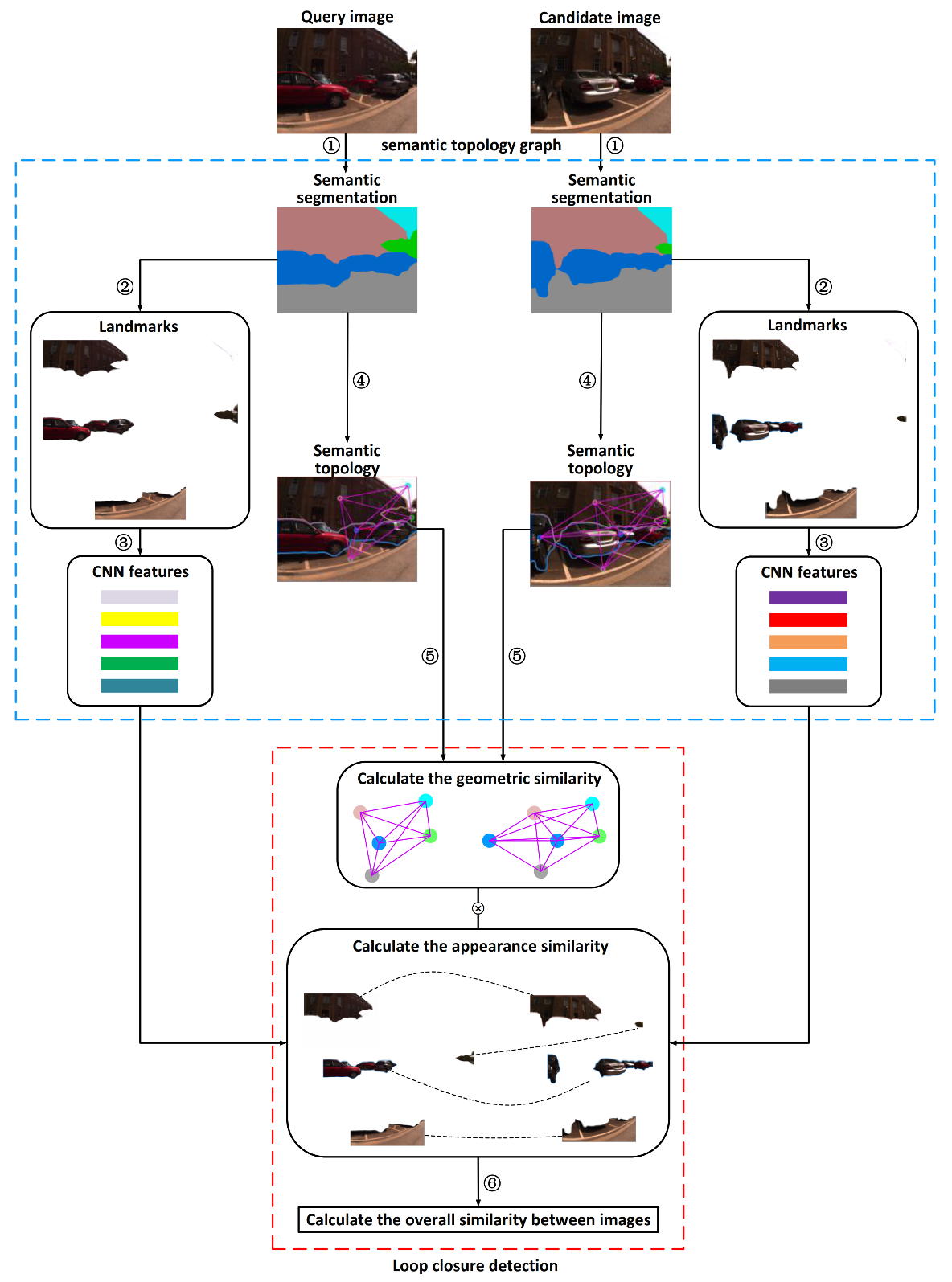
As shown in Figure 1, the algorithm of loop closure detection proposed in this paper includes the following key modules:
- (1)
- The extraction of the semantic landmarks.
- (2)
- The elimination of the dynamic landmarks and selection of the distinctive landmarks.
- (3)
- The calculation of the CNN features in landmark regions and dimensionality reduction processing on CNN features.
- (4)
- The construction of the semantic topological graphs and expression of random walk descriptors.
- (5)
- The calculation of geometric similarity with random walk descriptors.
- (6)
- The calculation overall similarity for loop closure detection.
Among the key steps, steps (1)–(4) are algorithms for constructing semantic topological graphs, which are given in Section 2.1, and steps (5) and (6) are loop closure detection algorithms, which are provided in Section 2.2.
The method presented in this paper is different from previous methods as follows:
- The extraction of the landmarks uses a pre-trained semantic segmentation network.
- It utilizes semantic information to eliminate dynamic landmarks and select of the distinctive landmarks.
- It adopts random walk descriptors to represent the topological graphs for graph matching.
- It adds geometric constraints on the basis of appearance similarity.
2.1. Semantic Topology Graph
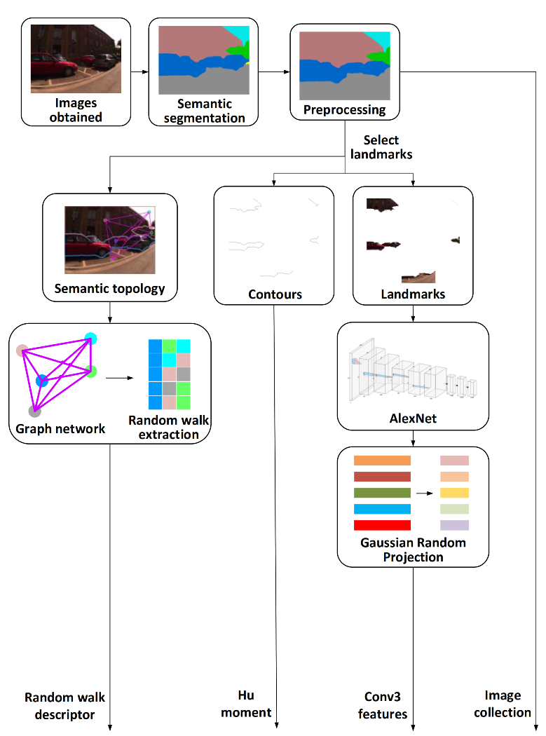
The construction of the semantic topology graphs is the basis of loop closure detection, so this section first introduces the construction process of the semantic topology graphs (see Figure 2).
For each obtained image, semantic segmentation is performed to extract landmarks. After preprocessing, the image is divided into landmark regions and contours. The obtained landmarks are selected and sent to AlexNet to extract third convolutional layer (Conv3) features. Then, Gaussian random projection is used to reduce the dimensionality of the feature vectors, and low-dimensional feature vectors are output. In addition, the Hu moment is calculated according to the obtained contours. At the same time, the preprocessed semantic segmentation images are used to extract the center of the landmark region as a node, and the landmarks seen from the same viewpoint are connected by undirected edges to establish a semantic topology graph according to the co-visibility information. Finally, a random walk descriptor is exploited to describe the topological graph structure. Here, the images obtained before the loop closure detection are called dataset images.
2.1.1. Landmark Extraction
Previous methods [30,31] have employed object proposal [42] to extract landmark regions even though it contains a lot of irrelevant feature information. In particular, the proposed method adopts semantic segmentation to extract landmarks, and this can accurately obtain the range of landmark regions.
DeepLabV3 + [43] is one of the most influential semantic segmentation models. It is better than FCN [44], U-Net [45], and SegNet [46] for some datasets, and it is widely used in the field of engineering technology. The ADE20K dataset [47,48] covers a wide range of scenes and object categories. Furthermore, it provides dense annotations, so it is used to train the DeepLabV3 +. The pre-trained DeepLabV3 + model can be applied for extracting landmarks.
Here, DeepLabV3 + was used to fuse the shallow features outputted by the encoder with the deep features generated from the ASPP module so that it could produce high-precision semantic segmentation results.
2.1.2. Landmark Selection
Due to the effects of illumination and dynamic disturbance in the images obtained by the robot, as well as the inherent defects of the semantic segmentation model, there was a lot of noise, as well as dynamic and secondary landmarks, in the semantic segmentation image that was obtained via the model discussed in Section 2.1.1. To overcome these problems, the landmarks were preprocessed to obtain significant landmark regions. Then, the dynamic regions from the landmarks obtained by preprocessing were removed, and the distinctive patches were selected.
As shown in Figure 3, the semantic segmentation image (see Figure 3b) was filtered to remove the regions; its area was less than the specified threshold (the threshold was 100 in this paper). Figure 3c was obtained by merging region filtered out with the surrounding area. Through the above-discussed procedures, the secondary landmarks and holes were filtered out to obtain the obvious landmark region with clear boundaries.
In order to overcome the impact of dynamic scenes, the semantic information of landmarks was then used to eliminate the pedestrian dynamic landmarks. At the same time, the pedestrians and long-term parking car region were merged, and the merged area could be used as car landmarks in subsequent work. Figure 3d was obtained by the above-mentioned operations. After excluding dynamic landmarks, in the follow-up loop closure detection, the dynamic landmarks were no longer matched. Furthermore, the number of pixels could be calculated for the landmark region. The distinctive landmarks were selected according to the number of landmark pixels and semantic information combined with experimental scenes for loop closure detection. In addition, dynamic landmarks were determined by scene content and landmark semantic information. In other words, according to the movement status of the landmarks in each experimental scene, we removed the moving landmarks in the dataset images and prevented them from participating in subsequent experiments. Formally, we denoted t as the number of distinctive landmarks selected in the image. (t was 5 or 10 in this work).
2.1.3. CNN Features
CNN features have appearance invariance, so they far surpass manual features in the field of image retrieval and classification. AlexNet [49] won the 2012 ImageNet competition champion, and the network was pre-trained for object recognition tasks on the ILSVRC dataset [50].
The AlexNet network architecture had 8 layers, of which the first 5 layers were convolutional layers and the last 3 layers were fully connected layers. There was a pooling layer after the 1st, 2nd, and 5th convolutional layers, but there was none after the 3rd and 4th convolutional layers. Each convolutional layer had activation function ReLU and normalization. The input of the network was a 227 × 227 3-channel image, and the output feature of the third convolutional layer was 13 × 13 × 384 = 64.896. According to the research of [27], the output features of the third convolutional layer of AlexNet perform best under appearance changes. We found that the output features of the fully connected layer had strong semantic information that was robust to viewpoint changes but poor for appearance changes. At the same time, it was proved that the AlexNex obtained by pre-training in the object recognition task was better than the CNN model based on place recognition training when considering the characteristics of the entire image under the viewpoint changes. Other advanced networks such as VGG, ResNet, and DenseNet have complex architectures, as well as a lack of research and utilization in the field of loop closure detection. Therefore, this article used the relatively lightweight and mature AlexNet in the loop closure detection field to extract CNN features. Based on the above research, the proposed method employed the output of the Conv3 of the AlexNet as the global feature in the landmark region.
The landmark proposal extracted by the object proposal method contained a large amount of irrelevant feature information. This led to a certain amount of noise influence in the CNN feature description. However, the landmark area extracted by semantic segmentation in this paper only contained the landmark feature and no other unrelated features. Figure 4a–c is introduced in Section 2.1.2, this section explains the landmark area and contour extraction. The landmarks from the filtering result (see Figure 4c) were selected to get Figure 4d, and the contour binary (Figure 4e) of the corresponding landmark was obtained by a Canny operator. Then, the landmarks (see Figure 4d) were resized to 227 × 227 pixels and input to the pre-trained AlexNet to extract features. As a result, the features of each landmark could be represented by a 64.896-dimensional vector. In order to keep the original size information of the landmark, this paper added the Hu moment of the contour (see Figure 4e) to the CNN feature to describe the landmark.
The obtained high-dimensional vector contained redundant landmark feature information, and a large amount of computational cost was required to calculate landmark similarity. Due to the real-time requirements of visual SLAM, the Gaussian random projection method [51] utilized in [30] was employed to reduce the dimensionality of the feature vector to 2048 dimensions.
2.1.4. Graph Representation
In order to preserve the spatial relationship of the scene, a semantic topology graph was constructed from a single image obtained by the robot. When the robot was initialized, the camera captured the first image and started to create the semantic topology graph. In this paper, each landmark was abstracted as a node containing category and pixel number information. Additionally, the node was located at the center of the landmark region.
The truncated random walk proposed by Perozzi et al. [52] was used to describe the semantic topological graph and represented each node as a fixed-length embedding vector. In order to enrich the feature expression, the node index and the number of pixels were adopted to describe the nodes. The node index was obtained according to the 150 semantic categories of the ADE20K dataset, and the number of pixels was acquired from the landmark region.
Then, the random walk descriptor of each node was calculated, and each node was used as the target node. In the semantic topological graph, the next adjacent node was randomly selected until the walking depth was reached and a random walking path was obtained. In this paper, random walks were performed on each node to obtain random walk paths. Finally, each target node could be expressed as a matrix . Since each node contained information about the index and the number of pixels, a matrix was finally obtained. In addition, the random walks followed certain rules, i.e., they would not repeat the same path and would not return to the previous nodes during each walk. The selection of and was related to the number of nodes in the graph structure. Based on the research of Gawel et al. [36] and the number of landmarks selected in Section 2.1.2, m was selected as 10, 20, or 50, and was 3 or 5 for experiments.
Figure 5 shows an example of a constructing descriptor. After the image in Figure 5a was obtained by the robot, the landmark nodes were extracted to obtain Figure 5b. Then, the nodes in Figure 5b were connected by undirected edges according to the co-visibility information to get Figure 5c. The semantic topology graph (see Figure 5d) was used to describe the geometric connection of the nodes in Figure 5a. Furthermore, a random walk graph descriptor (see Figure 5e) was constructed according to the semantic topology graph (see Figure 5d). The blue node (car) was used here to construct a descriptor for the target node. For the purpose of illustration, a graph description matrix was made to represent the geometric characteristics of the image by five random walks with a depth of 3 each time. The last row of Figure 5e corresponds to the random walk path shown by the black arrow in Figure 5d. Figure 5f used a matrix to quantify the description of Figure 5e, where the red box represents the index of nodes and the number of pixels. The index of the target node car was 21, and 68,192 was the number of pixels contained in the car landmark. In the same way, 2 and 112,918 were the index and pixel number of the building node, respectively; 3 and 13,488 were the index and pixel number of the sky node, respectively; 5 and 10,697 were the index and pixel number of the tree node, respectively; and 7 and 101,572 were the index and pixel number of the road node, respectively. For visualization, some node information was omitted.
2.2. Loop Closure Detection
This section introduces the algorithm of loop closure detection, and its flowchart is shown in Figure 6. Firstly, dataset images (candidate images) that matched the current image (query image) were retrieved. Then, the appearance similarity was calculated according to the CNN and contour features between images. In addition, geometric similarity was obtained by using the random walk descriptor. Finally, loop closure detection was performed according to the overall similarity.
2.2.1. Obtain Candidate Images
When the robot enters a previous environment again, it needs to retrieve the candidate images from the dataset images. In this article, by controlling the number of landmarks that shared the same label between the query image and each image in the dataset, candidate images of the current query image were obtained. The smaller the number of shared nodes, the more candidate images and the longer the retrieval time, and vice versa. A reasonable setting of the number of shared nodes can improve the speed and accuracy of loop closure detection, so the number of shared nodes was set as 1 to obtain candidate images. In other words, when both the query image and an image in the dataset images have a landmark with the same label, the dataset image is considered to be one candidate image. According to the same principle, each query image can obtain a candidate image set, and each image in the candidate image set has at least one landmark (node) with the same label as the query image.
2.2.2. Appearance Similarity
To calculate the appearance similarity between the candidate image and the current query image, it is necessary to match the landmark of the query image with all landmarks of the candidate image. By using the semantic information of landmarks, we employed the nearest neighbor search based on the cosine distance (see Equation (1)) of CNN features to match the landmark pairs of the same label in the two images so that only the landmarks of the same category were matched to speed up the matching process. In the matching process, we used a bidirectional matching method, i.e., landmark pairs were accepted only if they were mutual matches.
where denotes the feature vector of the i-th landmark of the query image and describes the feature vector of the j-th landmark of the candidate image.
While calculating the similarity of the CNN features, the geometric shape of the landmark was introduced as a penalty factor to eliminate the false positive phenomenon, i.e., the CNN features were similar but the contours were different. The references [30,31,53] used the difference between the long side and the wide side of the region proposal of the landmark pair to measure the shape difference. However, because they only used the long side and wide side difference of the bounding box, the influences of the scale and rotation was omitted. When the viewpoint changed drastically, the rotation of the landmark caused a large change in the aspect ratio of the bounding box. In the end, the shape penalty factor was too large, resulting in a low appearance similarity.
In order to solve the above problems, Hu moments [54] were used to describe the irregular contour features of landmarks, which possessed invariance about rotation, translation, and scale. Due to the wide range of Hu moments, the logarithm method was used for data compression in order to facilitate comparison. At the same time, considering that the Hu moment may have a negative value, absolute value was taken before the logarithm, as shown in Equation (2):
where is the sign function.
Hu [54] constructed seven invariant moments to describe geometric shape. Therefore, each landmark contour could be expressed as a feature vector by seven Hu moment values through Equation (3):
Through the contour feature vector, the shape difference of landmark contour between query image and candidate image could be calculated by Equation (4):
where and denote the m-th Hu moment of the i-th landmark contour in query image and the m-th Hu moment of the j-th landmark contour in candidate image, respectively.
According to cosine distance of the CNN feature and shape similarity obtained by the above calculation, the appearance similarity of the landmark pair between the query and the candidate images could be obtained by Equation (5):
In Equation (5), when the contour shape of the landmark is close, is close to 1. If is larger, it indicates that the contour difference of the landmark is large. In addition, when is close to 1, it means that the landmarks both have similar CNN features and geometric shapes. Furthermore, when is a negative number, it indicates that the geometric shapes of the landmarks differ greatly. If is small, it reveals that there may be differences in the CNN features or geometric shapes.
2.2.3. Geometric Similarity
In visual SLAM, the accuracy of loop closure detection is particularly important. Therefore, it is necessary to consider both appearance similarity and geometric similarity during loop closure detection. Thus, the random walk graph descriptor proposed in Section 2.1.4 was used to calculate geometric similarity for graph matching. Denote that the vectorized form of the descriptor matrix using is a concatenation of the columns of into a vector.
In Section 2.1.4, we obtained the random walk descriptor of the dataset images and only needed to construct the semantic topology graph to extract the descriptor for the query image. Since the number of pixels was much larger than the node index in value, the absolute size of the feature vector of the description changed greatly. Therefore, it was more appropriate to use cosine similarity to express the relative difference of graph descriptors by Equation (6):
where and denote the feature vector of the random walk descriptor in query image and candidate image, respectively. The denominator is the product of the corresponding vector modulus length. After getting a similarity score, it needed to be normalized with Equation (7):
Through Equation (7), the similarity score in the range of could be obtained.
2.2.4. Overall Similarity
This section discusses the calculation of the overall similarity between the query image and the candidate image. We not only considered the appearance characteristics of the image but also added geometric constraints. Section 2.2.2 and Section 2.2.3 obtained the appearance and geometric similarities of a single landmark pair. Through Equations (8) and (9), we scored each best matched landmark pair between the query image and the candidate image . The similarity score between each landmark in the query image and the most similar landmark selected by the nearest neighbor search method in the candidate image was first computed, and then the scores were assigned to the candidate image as the mean value of individual scores of its landmarks. Finally, through Equation (10), the overall similarity score of each candidate image was obtained.
where denotes the number of the landmarks in the candidate image (including unmatched landmarks), represents the i-th landmark of the current query image, and is the most similar landmark selected by the nearest neighbor search method in the candidate image. Moreover, the sum is done only on the best matched landmark pairs selected by the nearest neighbor search method.
In Equation (10), geometric similarity is used as a penalty factor for appearance similarity score to filter candidate images with similar local features but large differences in geometric information. In the experiments, it was normalized to . We normalized a set of overall similarity scores between the current query image and all candidate images (in Section 2.2.1). When the overall similarity score set of the current query image be , denotes the number of candidate images retrieved from the current query image. In addition, () denotes the overall similarity score between the current query image and the i-th candidate image. Through Equation (11), each value in can be normalized to :
where is the normalized score set and is one of the score values.
After obtaining the normalized similarity score for loop closure detection, it is often necessary to perform time and space consistency verification. In this article, the geometry check was not added. Nevertheless, the proposed method that integrates visual, spatial, and semantic information was still found to improve performance.
3. Results
This section mainly introduces the experimental process and result analysis. In order to evaluate the performance of different components of the proposed method and to compare the performance of the proposed method with other state-of-the-art methods, the following methods were considered:
- (1)
- A state-of-the-art BoW-based method (named ‘DBoW2′) that did not need to recreate the vocabulary in different scenarios [11].
- (2)
- A CNN approach (named ‘Conv3′) that applied the global Conv3 feature to describe images [27].
- (3)
- A technique (named ‘CNNWL’) that combined global and local CNN features but ignored the spatial relationship of landmarks [30].
- (4)
- An approach (named ‘GOCCE’) that was based on local features and semi-semantic information [31]. It was closer to the proposed algorithm.
- (5)
- The proposed complete method (named ‘VSSTC’) that integrated visual, spatial, and semantic information through topological graphs and CNN features.
- (6)
- Two simplified versions of the random walk graph descriptor of our method. One version included only label information (named ‘VSSTC-Label’), and the other used only pixel number information (named ‘VSSTC-Pixel’).
- (7)
- A modified version of our method of landmark segmentation method (named ‘VSSTC-OP’) that used object proposal instead of semantic segmentation to extract landmark regions, while using the size of the bounding box instead of Hu moments.
- (8)
- Another reduced version of our method (named ‘VSSTC-LS’) that did not construct topological graphs and lacks spatial information. In order to compare the performance of the proposed method with that of the above methods, comparative experiments were carried out on the datasets and a mobile robot. Based on the experimental results, the proposed method was fully evaluated.
In the experiments, a precision–recall curve (P–R curve) [55] was used as a quantitative evaluation metric, as it is a standard metric for loop closure detection results. By changing the similarity threshold, the P–R curve could be obtained. In order to further observe the experimental results, the maximum recall rate under the precision of 100% and the area (the value in ) under the P–R curve (AUC) were used as auxiliary evaluation metrics. The larger the recall rate and the area, the better the performance.
The experiments were carried out on a desktop equipped with GTX 1080Ti GPU. We used a pre-trained DeepLabV3 + based on the TensorFlow [56] for semantic segmentation and AlexNet based on Caffe [57] to extract CNN features.
3.1. Dataset Experiments
3.1.1. Datasets
The performance evaluation was performed through the following four public datasets, which are widely used in the field of loop closure detection and place recognition.
City Centre dataset: This dataset [10] contains 1237 pairs of images in outdoor urban environments. The resolution of each image is 640 × 480. It contains dynamic scenes of pedestrians and vehicles. In addition, there are a lot of scenes with changes in viewpoint caused by lateral displacement and reverse movement. It also includes shadows and spots caused by lighting. Ground truth data are included in the dataset. In the experiment, six types of landmarks were selected: tree, road, sky, building, car, and grass. Furthermore, person and bicycle dynamic landmarks were excluded. The dataset scenario is listed in Figure 7a.
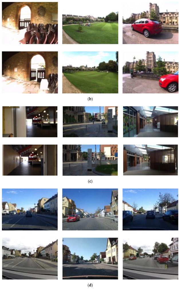
New College dataset: This dataset [10] contains 1073 pairs of images of a university campus, which contains a small number of dynamic scenes of pedestrians and vehicles. Additionally, it includes the scenes of viewpoint changes caused by lateral displacement. Furthermore, there are many indoor repetitive structures, such as walls, chairs, and windows. The resolution of each image is 640 × 480. Ground truth data are included in the dataset. In the experiments, eight types of landmarks—sky, wall, chair, building, road, grass, tree, and car—were selected and the person landmark was excluded. The scenes of the dataset images are shown in Figure 7b.
Gardens Point dataset: This dataset has been used in [27] before and is available online (http://tinyurl.com/gardenspointdataset) which contains two traversals on the university campus during the day, one route on the left-hand side of the road and the other on the right-hand side of the road on the same day. In addition, the dataset includes 200 pairs of images, with the left and right sides of the road each containing 200 images. It contains the viewpoint changes caused by walking on the left and right sides of the road, and there are many pedestrian dynamic objects. Ground truth data are included in the dataset. In the experiment, we selected eight types of landmarks: wall, building, sky, road, flooring, door, tree, and ceiling. The person landmark was excluded. The scenes within dataset images are shown in Figure 7c.
Mapillary dataset: The Mapillary datasets were first introduced by [30] and is available online (http://www.mapillary.com) they have street-level imagery and map data from all over the world. We downloaded the Berlin August–Bebel–Straße sequence, as well as ground truth data, to get 318 images. The dataset exhibits significant changes in viewpoints and severe changes in appearance. In addition, it contains a large number of moving vehicle dynamic objects. We selected six types of landmarks—building, road, sky, tree, pole, and signal—and excluded car landmarks. Some images in the dataset are shown in Figure 7d.
3.1.2. Experimental Results and Analysis
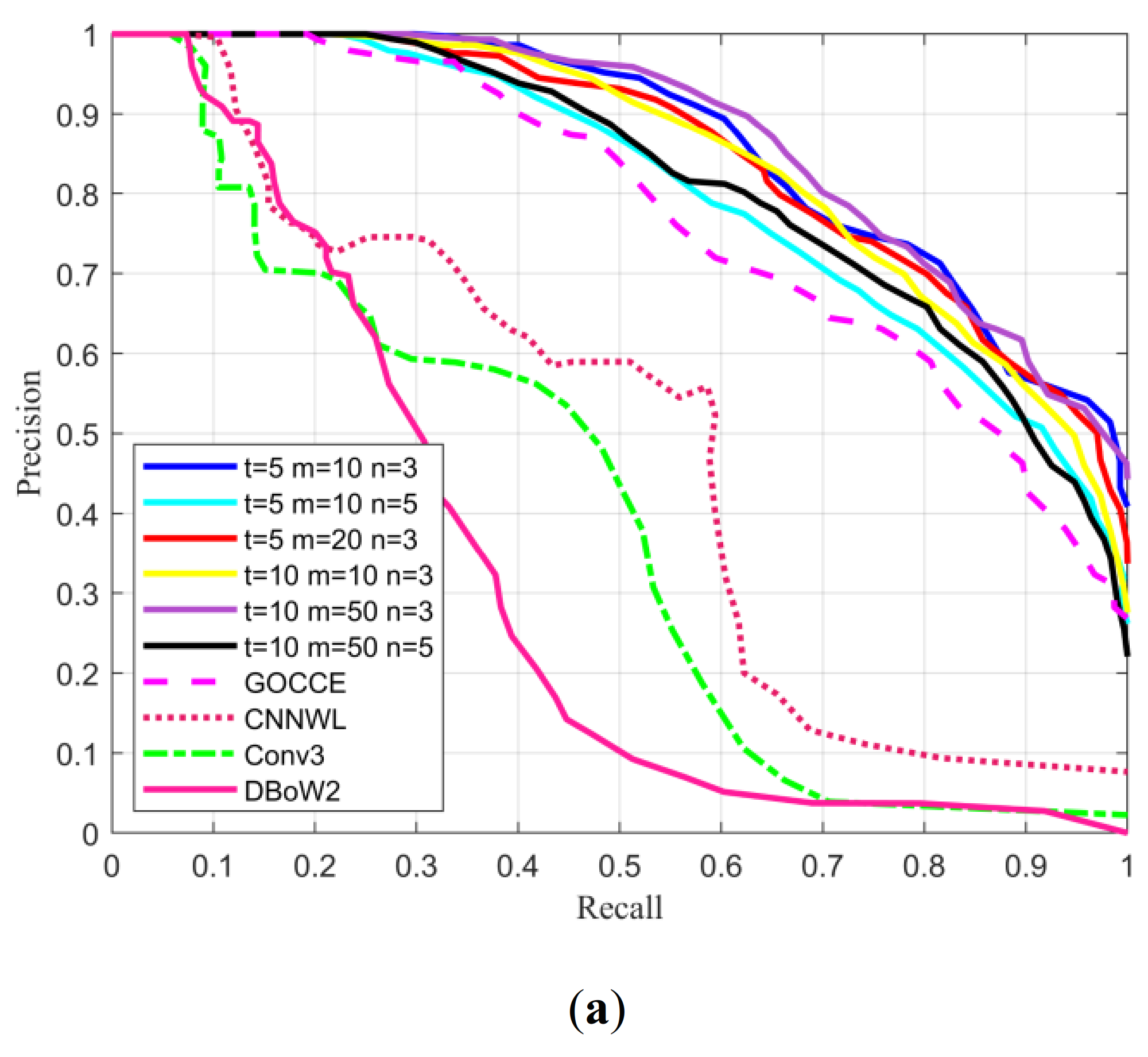
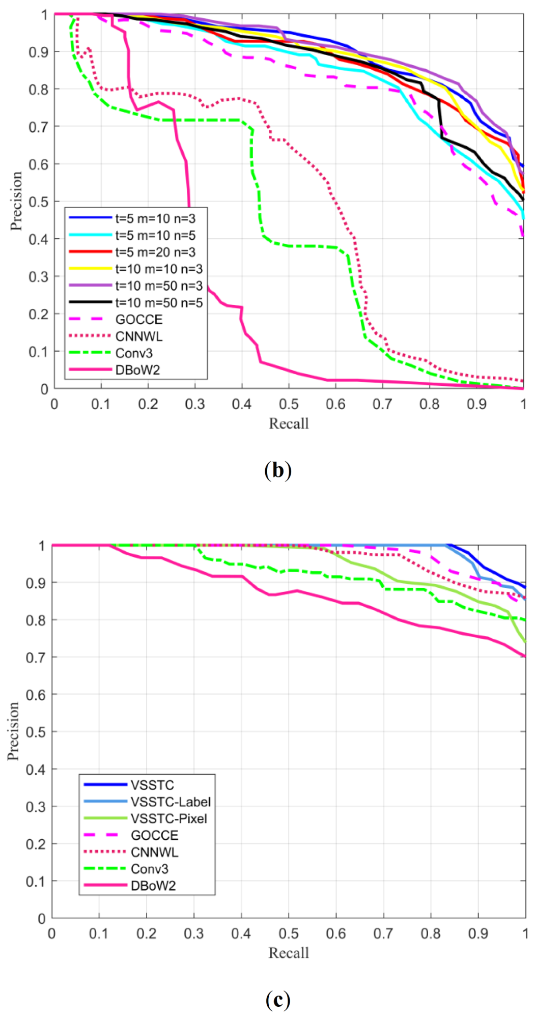
The experiments not only illustrated the experimental effects of the proposed approach under different parameter settings but also provided comparison results with other advanced methods. In order to test the topological graph descriptor of the proposed method, the experiments (Figure 8a,b) were conducted by extracting the number of different landmarks ( or 10), using different random walks (, 20, or 50) and walk depth ( or 5) to change the size of the graph representation. In addition, the proposed complete method was fully compared with other methods (Figure 8). Moreover, we conducted ablation studies (Figure 8c,d) on the components of the proposed system to analyze the performance of each component. Among them, we analyzed the influence of the composition factors of the topological graph descriptors in the proposed method (Figure 8c). The VSSTC-Label method only considered the landmark label, and the VSSTC-Pixel approach only used the number of pixels. These two methods and the proposed VSSTC method were tested on the Gardens Point dataset. In addition, to verify the proposed landmark region extraction method (VSSTC), we replaced the landmark segmentation method with the object proposal method (VSSTC-OP) instead of semantic segmentation to obtain bounding boxes (Figure 8d). At the same time, this experiment verified the effectiveness of Hu moments relative to the size of the bounding box on the Mapillary dataset. Furthermore, to consider the impact of the semantic topology graph on the performance of the proposed method, the removed topology graphs (VSSTC-LS) and the complete method (VSSTC) were analyzed in the mobile robot experiment (see Section 3.2). Figure 8 shows the P–R curves of the experimental results, and Table 1 and Table 2 list the maximum recall rate under the precision of 100% and the area under the P–R curve.
From the P–R curves in Figure 8, we can see that in the case of graph descriptor size and , the maximum recall rate of was larger than that of . This shows that blindly increasing the number of landmarks can entrain many minor landmarks to participate in loop closure detection, thereby weakening performance. In addition, whether in the case of , , or , , the maximum recall rate at exceeded that at . This indicates that when the walk depth reached the graph size limit, continuing to increase the walk depth made the model visit the nodes that had been visited before. This reduced the ability to express the graph descriptor and diminished the loop closure detection performance. Furthermore, in the case of and , the maximum recall rate when was larger than that when . However, in the case of and , the maximum recall rate when was larger than that when . This demonstrates that the number of random walks was determined by the size of the semantic topology graph. When the size of the semantic topology graph was small, too large a number of walks reduced the performance of the graph descriptor. When the size of the semantic topology graph was small, a large number of random walk times caused the model to access repeated paths, thereby reducing performance. However, appropriately increasing the number of random walk times according to the size of the semantic topology graph improved the expressive ability of the graph descriptor. In summary, when , and , the effect of loop closure detection achieved a good compromise between accuracy and complexity. In order to further clarify the experimental results, it can be observed from Table 1 that the maximum recall rate and AUC value in the City Centre and New College datasets also conformed to the above conclusions.
From the experimental results on the City Centre and New College datasets, it can be seen that the performance of the DBoW2 method was the worst. Moreover, this method was inferior to other methods based on CNN features. This shows that the traditional BoW method based on manual features was poor in robustness and could only deal with limited scenarios. In addition, the CNNWL method was better than the Conv3 one. This shows that the CNNWL method that combined global and local CNN features had better graph description capabilities than that of the global CNN feature method. Furthermore, the performance of the proposed VSSTC method significantly exceeded that of the CNNWL method. This demonstrates that the proposed method with added spatial constraints had better performance. This also proves that the random walk descriptor based on the semantic topological graph proposed in this paper had an excellent graph description ability. Importantly, our method outperformed the GOCCE one, which shows the advantages of the proposed semantic topology graph in the face of viewpoint changes and dynamic scenes.
The authors of this article conducted three groups of ablation studies to analyze the impact of each component of the proposed method on the overall performance. From Figure 8c and Table 2, we can see that the VSSTC-Label method had better performance than the VSSTC-Pixel approach, which underlines the importance of landmark label information in the topology graph descriptor. In addition, it could be seen that the performance of VSSTC-Pixel method was inferior to that of the GOCCE method, which shows that the performance of graph descriptors lacking semantic information dropped sharply. Furthermore, the VSSTC method had the best performance, which also reflects that the performance of the proposed complete method was greatly improved by integrating the landmark label and pixel number information.
From Figure 8d and Table 2, we can understand that the performance of the VSSTC-OP method was inferior to that of the VSSTC method, which reveals the superiority of using semantic segmentation to extract landmark regions and employing Hu moments to represent region shape information. As expected, the bounding box extracted by region proposal extracted interference features when facing the presence of a complex background, resulting in performance degradation. The remaining ablation research is given when discussing the mobile robot experiment.
3.2. Mobile Robot Experiment
In order to further verify the robustness of the proposed method to viewpoint changes and dynamic scenes, experiments were carried out in outdoor scenes using the mobile robot of our team.
3.2.1. Experimental Platform
As shown in Figure 9, we used a wheel–leg hybrid hexapod robot with a length of 2 m, a width of 1.7 m, and a height of 1 m as the experimental platform. Moreover, the robot was equipped with an Intel Braswell processor and a centimeter-level integrated navigation system. We used a controller to remotely control the robot and drive 1.5 km in the campus of Xidian University. The data were captured by the front YAMAKO camera (see Figure 9b) for the experiment. In the mobile robot experiment, with a focal length of 10 mm and a working distance of 15 m, a field of view of approximately 9600 × 7200 mm could be obtained. The detailed parameters of the YAMAKO camera are shown in Table 3. Finally, 108,000 frames of images were collected at a video frame rate of 30 Hz. By setting the distance threshold of the obtained image sequence to 2 m, 720 key frames could be obtained. In addition, the obtained frames were perfectly aligned by the GPS information, which could be used as the ground truth of loop closure detection.
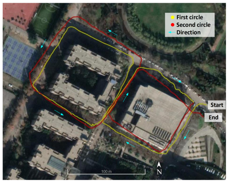
As seen in Figure 10, the trajectory of the robot was recorded by the GNSS and INS integrated positioning system. The robot drove two laps; the first lap was obtained by driving along the left side of the road, and the second lap was acquired by driving along the right side of the road in the same direction as the first lap. The experimental scene contained changes in viewpoint caused by the lateral displacement and also included a lot of dynamic scenes. In addition, it included a lot of shadows and bright spots caused by light. The experiment selected four types of landmarks: road, building, tree, and sky. Furthermore, the dynamic landmarks of person, bicycle, and car were excluded.
3.2.2. Experimental Results and Analysis
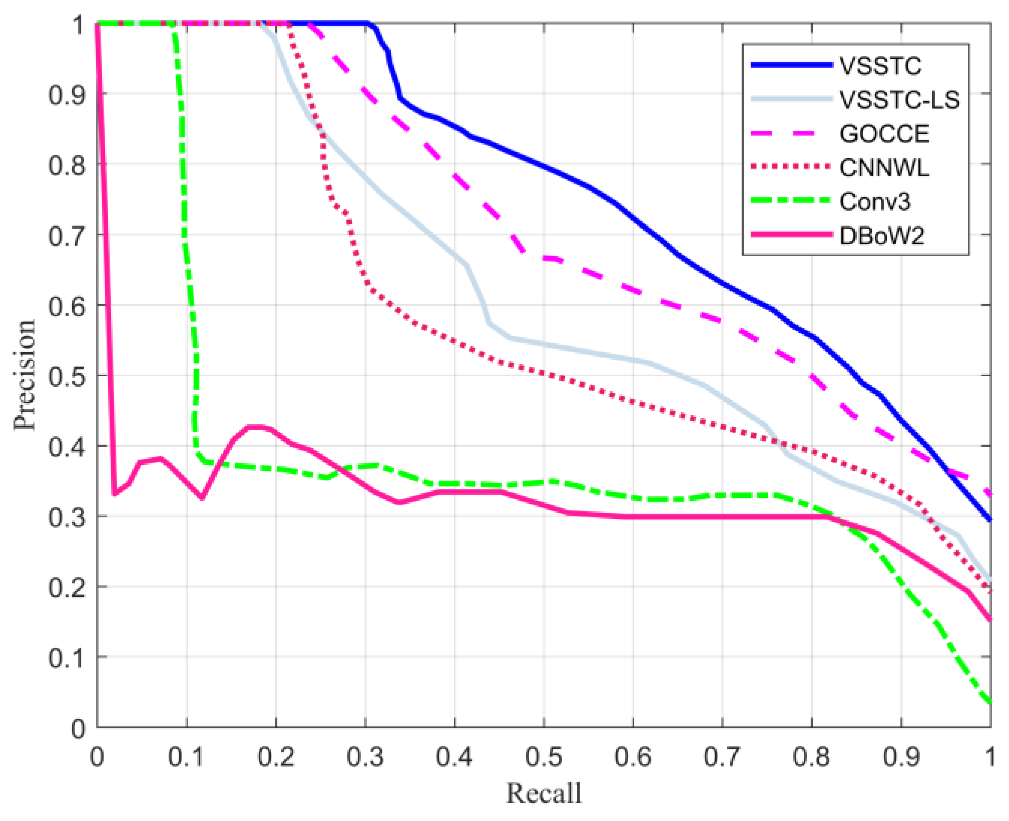
Figure 11 shows the P–R curves of the mobile robot, and Table 2 lists the maximum recall rate under the precision of 100% and the area under the P–R curve. According to Section 3.1.2, 5, , and were used as the random walk descriptor parameters of the proposed method. In Figure 11 and Table 2, it can be seen that the DBoW2 method performed the worst. A possible reason for this performance is that the experimental scene contained a large number of viewpoint changes and dynamic scenes. Moreover, the CNNWL method had better performance than the Conv3 one, which shows that the CNNWL method was more robust for expressing the image by considering both global and local features in the viewpoint changes and dynamic scenes. Furthermore, the proposed VSSTC method performed better than the CNNWL and GOCCE methods, thus demonstrating that the spatial and semantic information played an important role in improving the loop closure detection performance of changing viewpoint and dynamic scenes.
More importantly, from Figure 11 and Table 2, it can be seen from the experimental results that the VSSTC-LS method had a much poorer performance than the VSSTC method that considered spatial information. This shows that the spatial geometric information had a greater impact on loop closure detection performance. In addition, we can see that the performance of the VSSTC-LS method was slightly better than that of the CNNWL method, which reflects that the visual and semantic modules used in the proposed method were superior when there was no geometric information.
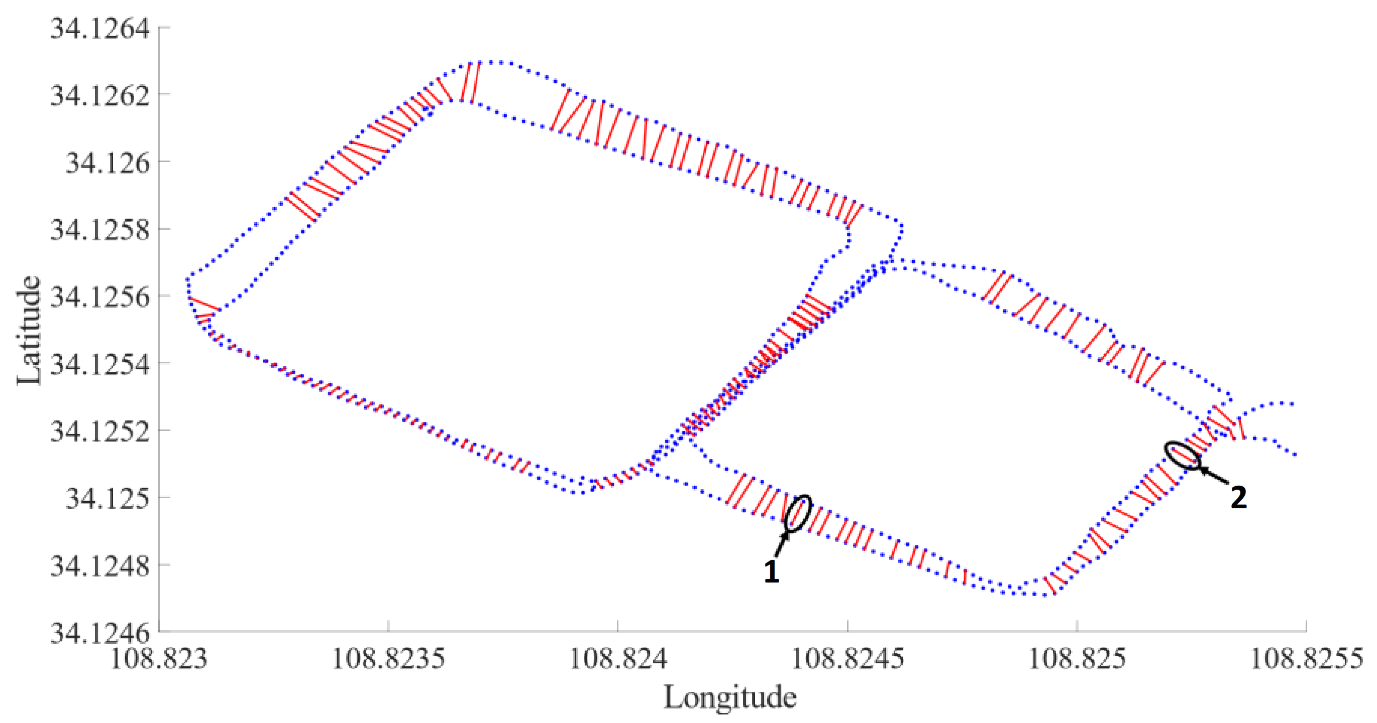
Figure 12 shows a loop closure detection result obtained by the proposed method. The blue points are the selected 720 key-frames, and the key-frames connected by the red line indicate the correct loop closure. It can be seen from the figure that the proposed method could still detect a large number of loop closures under the influence of viewpoint changes and dynamic scenes. Figure 13a,b shows the true positive image pairs detected by loop closure detection at 1 and 2 in Figure 12, respectively. Figure 13a,b contains viewpoint changes and pedestrian dynamic scenes, as well as the shadows caused by the changes in illumination. This shows that the proposed method had a better graph description ability in the above-mentioned drastically changing scenes.
4. Conclusions
This paper studied the loop closure detection in visual SLAM and proposed a robust loop closure detection method that integrated visual–spatial–semantic information to deal with viewpoint changes and dynamic scenes. Firstly, semantic topological graphs were employed to represent the spatial geometric relationships of landmarks, and random walk descriptors were applied to represent topological graphs. By adding geometric constraints, the mismatch problem caused by changes in viewpoint was improved. Then, semantic information was utilized to eliminate dynamic landmarks, and distinctive landmarks were selected for loop closure detection, which effectively alleviated the impact of dynamic scenes. Finally, semantic segmentation was used of accurately obtain the landmark region. At the same time, deep learning was adopted to automatically learn the complex internal features of landmarks without the need to manually design features. As a result, it eased the effect of appearance changes. According to the experimental results of the datasets and a mobile robot, the proposed method can effectively cope with changes in viewpoint and dynamic scenes.
However, the proposed method has certain limitations. Firstly, the pros and cons of using semantic segmentation to extract landmark regions depend on the selection of the semantic segmentation model and pre-training datasets. When using this approach, the users need to select a semantic segmentation model according to experimental scenes. At the same time, the model was trained by fine-tuning and transfer learning. Second, this work was offline. It takes a certain amount of time to extract landmark regions and obtain CNN features. In future research, we will try other segmentation models to extract semantic landmarks and use more comprehensive and complete datasets to train the segmentation network so that the model can cope with changing experimental scenarios. Furthermore, this paper used a single image to construct a semantic topology graph. In the future, we will construct a topology graph for sequence images to improve loop closure detection performance. In addition, the proposed strategy for selecting representative landmarks still has room for improvement. To further explore more suitable representative landmark selection strategies, we plan to divide landmarks into the four categories of dynamic, static, unreliable segmentation, and ubiquitous landmarks based on indoor and outdoor scenes while considering the differences between urban and rural scenes. Then, we will assign weights to each type of landmark according to different dataset scenarios to improve our work. Furthermore, in the experimental part, in order to conduct ablation studies, we designed different combinations of the proposed methods, and there is still room for the optimization of these combinations. To further explore the effect of each component of the proposed method on overall performance, we will design more diversified and rigorous ways of measurements to improve the work of this article.
Author Contributions
Conceptualization, Y.W. and Y.Q.; methodology, Y.W., Y.Q. and P.C.; software, Y.W.; resources, X.D. and P.C.; writing—original draft preparation, Y.W.; writing—review and editing, Y.Q. and P.C.; supervision, Y.Q. and X.D. All authors have read and agreed to the published version of the manuscript.
Funding
This research was funded by the National Natural Science Foundation of China under Grant 61871308, the Natural Science Basic Research Plan in Shaanxi Province of China under Grant 2019JM-426.
Acknowledgments
We thank Mark Cummins for providing the City Centre, New College datasets. In addition, we are also very grateful for the Gardens Point dataset provided by QUT. We are also very grateful for the dataset provided by the open source map service of Mapillary.
Conflicts of Interest
The authors declare no conflict of interest.
References
- Smith, R.C.; Cheeseman, P. On the representation and estimation of spatial uncertainty. Int. J. Robot. Res. 1986, 5, 56–68. [Google Scholar] [CrossRef]
- Palomeras, N.; Carreras, M.; Andrade-Cetto, J. Active SLAM for autonomous underwater exploration. Remote Sens. 2019, 11, 2827. [Google Scholar] [CrossRef] [Green Version]
- Chiang, K.-W.; Tsai, G.-J.; Li, Y.-H.; Li, Y.; El-Sheimy, N. Navigation Engine Design for Automated Driving Using INS/GNSS/3D LiDAR-SLAM and Integrity Assessment. Remote Sens. 2020, 12, 1564. [Google Scholar] [CrossRef]
- Ho, K.L.; Newman, P. Detecting loop closure with scene sequences. Int. J. Comput. Vis. 2007, 74, 261–286. [Google Scholar] [CrossRef]
- Folkesson, J.; Christensen, H. Graphical SLAM-a self-correcting map. In Proceedings of the IEEE International Conference on Robotics and Automation, New Orleans, LA, USA, 26 April–1 May 2004; pp. 383–390. [Google Scholar]
- Thrun, S.; Montemerlo, M. The Graph SLAM Algorithm with Applications to Large-Scale Mapping of Urban Structures. Int. J. Robot. Res. 2006, 25, 403–429. [Google Scholar] [CrossRef]
- Grisetti, G.; Kümmerle, R.; Stachniss, C.; Burgard, W. A tutorial on graph-based SLAM. IEEE Intell. Transp. Syst. Mag. 2010, 2, 31–43. [Google Scholar] [CrossRef]
- Triggs, B.; McLauchlan, P.F.; Hartley, R.I.; Fitzgibbon, A.W. Bundle adjustment—a modern synthesis. In Proceedings of the International workshop on vision algorithms, Berlin/Heidelberg, Germany, 21–22 September 1999; pp. 298–372. [Google Scholar]
- Williams, B.; Klein, G.; Reid, I. Automatic Relocalization and Loop Closing for Real-Time Monocular SLAM. IEEE Trans. Pattern Anal. Mach. Intell. 2011, 33, 1699–1712. [Google Scholar] [CrossRef]
- Cummins, M.; Newman, P. FAB-MAP: Probabilistic localization and mapping in the space of appearance. Int. J. Robot. Res. 2008, 27, 647–665. [Google Scholar] [CrossRef]
- Gálvez-López, D.; Tardos, J.D. Bags of binary words for fast place recognition in image sequences. IEEE Trans. Robot. 2012, 28, 1188–1197. [Google Scholar] [CrossRef]
- Lowe, D.G. Distinctive Image Features from Scale-Invariant Keypoints. Int. J. Comput. Vis. 2004, 60, 91–110. [Google Scholar] [CrossRef]
- Bay, H.; Ess, A.; Tuytelaars, T.; Gool, L.V. Speeded-Up Robust Features (SURF). Comput. Vis. Image Underst. 2008, 110, 346–359. [Google Scholar] [CrossRef]
- Rublee, E.; Rabaud, V.; Konolige, K.; Bradski, G. ORB: An efficient alternative to SIFT or SURF. In Proceedings of the 2011 International Conference on Computer Vision, Barcelona, Spain, 6–13 November 2011; pp. 2564–2571. [Google Scholar]
- Angeli, A.; Filliat, D.; Doncieux, S.; Meyer, J. Fast and Incremental Method for Loop-Closure Detection Using Bags of Visual Words. IEEE Trans. Robot. 2008, 24, 1027–1037. [Google Scholar] [CrossRef] [Green Version]
- Labbe, M.; Michaud, F. Online global loop closure detection for large-scale multi-session graph-based SLAM. In Proceedings of the IEEE/RSJ International Conference on Intelligent Robots and Systems, Chicago, IL, USA, 14–18 September 2014; pp. 2661–2666. [Google Scholar]
- Mur-Artal, R.; Tardós, J.D. Orb-slam2: An open-source slam system for monocular, stereo, and rgb-d cameras. IEEE Trans. Robot. 2017, 33, 1255–1262. [Google Scholar] [CrossRef] [Green Version]
- Sünderhauf, N.; Protzel, P. Brief-gist-closing the loop by simple means. In Proceedings of the IEEE/RSJ International Conference on Intelligent Robots and Systems, San Francisco, CA, USA, 25–30 September 2011; pp. 1234–1241. [Google Scholar]
- Oliva, A.; Torralba, A. Modeling the Shape of the Scene: A Holistic Representation of the Spatial Envelope. Int. J. Comput. Vis. 2001, 42, 145–175. [Google Scholar] [CrossRef]
- Naseer, T.; Spinello, L.; Burgard, W.; Stachniss, C. Robust visual robot localization across seasons using network flows. In Proceedings of the Twenty-Eighth AAAI Conference on Artificial Intelligence, Québec City, QC, Canada, 27–31 July 2014; pp. 2564–2570. [Google Scholar]
- Milford, M.J.; Wyeth, G.F. SeqSLAM: Visual route-based navigation for sunny summer days and stormy winter nights. In Proceedings of the IEEE International Conference on Robotics and Automation, Saint Paul, MN, USA, 14–18 May 2012; pp. 1643–1649. [Google Scholar]
- Abdollahyan, M.; Cascianelli, S.; Bellocchio, E.; Costante, G.; Ciarfuglia, T.A.; Bianconi, F.; Smeraldi, F.; Fravolini, M.L. Visual localization in the presence of appearance changes using the partial order kernel. In Proceedings of the European Signal Processing Conference, Rome, Italy, 3–7 September 2018; pp. 697–701. [Google Scholar]
- Pepperell, E.; Corke, P.I.; Milford, M.J. All-environment visual place recognition with SMART. In Proceedings of the IEEE International Conference on Robotics and Automation, Hong Kong, China, 31 May–7 June 2014; pp. 1612–1618. [Google Scholar]
- Hansen, P.; Browning, B. Visual place recognition using HMM sequence matching. In Proceedings of the IEEE/RSJ International Conference on Intelligent Robots and Systems, Chicago, IL, USA, 14–18 September 2014; pp. 4549–4555. [Google Scholar]
- Xia, Y.; Jie, L.; Lin, Q.; Hui, Y.; Dong, J. An Evaluation of Deep Learning in Loop Closure Detection for Visual SLAM. In Proceedings of the 2017 IEEE International Conference on Internet of Things and IEEE Green Computing and Communications and IEEE Cyber, Physical and Social Computing and IEEE Smart Data, Exeter, UK, 21–23 June 2017; pp. 85–91. [Google Scholar]
- Hou, Y.; Zhang, H.; Zhou, S. Convolutional neural network-based image representation for visual loop closure detection. In Proceedings of the IEEE International Conference on Information and Automation, Lijiang, China, 8–10 August 2015; pp. 2238–2245. [Google Scholar]
- Sünderhauf, N.; Shirazi, S.; Dayoub, F.; Upcroft, B.; Milford, M. On the performance of ConvNet features for place recognition. In Proceedings of the IEEE/RSJ International Conference on Intelligent Robots and Systems, Hamburg, Germany, 28 September–2 October 2015; pp. 4297–4304. [Google Scholar]
- Arroyo, R.; Alcantarilla, P.F.; Bergasa, L.M.; Romera, E. Fusion and Binarization of CNN Features for Robust Topological Localization across Seasons. In Proceedings of the IEEE/RSJ International Conference on Intelligent Robots and Systems, Daejeon, South Korea, 9–14 October 2016; pp. 4656–4663. [Google Scholar]
- Gao, X.; Zhang, T. Unsupervised learning to detect loops using deep neural networks for visual SLAM system. Auton. Robot. 2017, 41, 1–18. [Google Scholar] [CrossRef]
- Sünderhauf, N.; Shirazi, S.; Jacobson, A.; Dayoub, F.; Pepperell, E.; Upcroft, B.; Milford, M. Place recognition with convnet landmarks: Viewpoint-robust, condition-robust, training-free. Robot. Sci. Syst. 2015, 1–10. [Google Scholar]
- Cascianelli, S.; Costante, G.; Bellocchio, E.; Valigi, P.; Fravolini, M.L.; Ciarfuglia, T.A. Robust visual semi-semantic loop closure detection by a covisibility graph and CNN features. Robot. Auton. Syst. 2017, 92, 53–65. [Google Scholar] [CrossRef]
- Finman, R.; Paull, L.; Leonard, J.J. Toward object-based place recognition in dense rgb-d maps. In Proceedings of the ICRA Workshop Visual Place Recognition in Changing Environments, Seattle, WA, USA, 26–30 May 2015. [Google Scholar]
- Oh, J.; Jeon, J.; Lee, B. Place recognition for visual loop-closures using similarities of object graphs. Electron. Lett. 2014, 51, 44–46. [Google Scholar] [CrossRef]
- Pepperell, E.; Corke, P.; Milford, M. Routed roads: Probabilistic vision-based place recognition for changing conditions, split streets and varied viewpoints. Int. J. Robot. Res. 2016, 35, 1057–1179. [Google Scholar] [CrossRef] [Green Version]
- Stumm, E.; Mei, C.; Lacroix, S.; Chli, M. Location graphs for visual place recognition. In Proceedings of the IEEE International Conference on Robotics and Automation, Seattle, WA, USA, 26–30 May 2015; pp. 5475–5480. [Google Scholar]
- Gawel, A.R.; Don, C.D.; Siegwart, R.; Nieto, J.; Cadena, C. X-View: Graph-Based Semantic Multi-View Localization. IEEE Robot. Autom. Lett. 2018, 3, 1687–1694. [Google Scholar] [CrossRef] [Green Version]
- Stumm, E.; Mei, C.; Lacroix, S.; Nieto, J.; Siegwart, R. Robust Visual Place Recognition with Graph Kernels. In Proceedings of the IEEE Conference on Computer Vision and Pattern Recognition, Las Vegas, NV, USA, 27–30 June 2016; pp. 4535–4544. [Google Scholar]
- Han, F.; Wang, H. Learning integrated holism-landmark representations for long-term loop closure detection. In Proceedings of the 32nd AAAI Conference on Artificial Intelligence, New Orleans, LA, USA, 2–7 February 2018; pp. 6501–6508. [Google Scholar]
- Chen, Z.; Maffra, F.; Sa, I.; Chli, M. Only look once, mining distinctive landmarks from convnet for visual place recognition. In Proceedings of the IEEE/RSJ International Conference on Intelligent Robots and Systems, Vancouver, BC, Canada, 24–28 September 2017; pp. 9–16. [Google Scholar]
- Schönberger, J.L.; Pollefeys, M.; Geiger, A.; Sattler, T. Semantic visual localization. In Proceedings of the IEEE Conference on Computer Vision and Pattern Recognition, Salt Lake City, UT, USA, 18–22 June 2018; pp. 6896–6906. [Google Scholar]
- Gao, P.; Zhang, H. Long-Term Loop Closure Detection through Visual-Spatial Information Preserving Multi-Order Graph Matching. In Proceedings of the Thirty-Fourth AAAI Conference on Artificial Intelligence, New York, NY, USA, 7–12 February 2020; pp. 10369–10376. [Google Scholar]
- Zitnick, C.L.; Dollár, P. Edge boxes: Locating object proposals from edges. In Proceedings of the European Conference on Computer Vision, Zurich, Switzerland, 6–12 September 2014; pp. 391–405. [Google Scholar]
- Chen, L.-C.; Zhu, Y.; Papandreou, G.; Schroff, F.; Adam, H. Encoder-decoder with atrous separable convolution for semantic image segmentation. In Proceedings of the European conference on computer vision, Munich, Germany, 8–14 September 2018; pp. 801–818. [Google Scholar]
- Long, J.; Shelhamer, E.; Darrell, T. Fully convolutional networks for semantic segmentation. In Proceedings of the IEEE Conference on Computer Vision and Pattern Recognition, Boston, Mass, USA, 7–13 June 2015; pp. 3431–3440. [Google Scholar]
- Ronneberger, O.; Fischer, P.; Brox, T. U-net: Convolutional networks for biomedical image segmentation. In Proceedings of the International Conference on Medical image computing and computer-assisted intervention, Munich, Germany, 5–9 October 2015; pp. 234–241. [Google Scholar]
- Badrinarayanan, V.; Kendall, A.; Cipolla, R. Segnet: A deep convolutional encoder-decoder architecture for image segmentation. IEEE Trans. Pattern Anal. Mach. Intell. 2017, 39, 2481–2495. [Google Scholar] [CrossRef]
- Zhou, B.; Zhao, H.; Puig, X.; Xiao, T.; Fidler, S.; Barriuso, A.; Torralba, A. Semantic understanding of scenes through the ade20k dataset. Int. J. Comput. Vis. 2019, 127, 302–321. [Google Scholar] [CrossRef] [Green Version]
- Zhou, B.; Zhao, H.; Puig, X.; Fidler, S.; Barriuso, A.; Torralba, A. Scene parsing through ade20k dataset. Proceedings of IEEE Conference on Computer Vision and Pattern Recognition, Honolulu, HI, USA, 21–26 July 2017; pp. 633–641. [Google Scholar]
- Krizhevsky, A.; Sutskever, I.; Hinton, G.E. Imagenet classification with deep convolutional neural networks. In Proceedings of the Advances in neural information processing systems, Lake Tahoe, NV, USA, 3–6 December 2012; pp. 1097–1105. [Google Scholar]
- Russakovsky, O.; Deng, J.; Su, H.; Krause, J.; Satheesh, S.; Ma, S.; Huang, Z.; Karpathy, A.; Khosla, A.; Bernstein, M. Imagenet large scale visual recognition challenge. Int. J. Comput. Vis. 2015, 115, 211–252. [Google Scholar] [CrossRef] [Green Version]
- Candes, E.J.; Tao, T. Near-optimal signal recovery from random projections: Universal encoding strategies? IEEE Trans. Inf. Theory 2006, 52, 5406–5425. [Google Scholar] [CrossRef] [Green Version]
- Perozzi, B.; Al-Rfou, R.; Skiena, S. Deepwalk: Online learning of social representations. In Proceedings of the 20th ACM SIGKDD international conference on Knowledge discovery and data mining, New York, USA, 24–27 August 2014; pp. 701–710. [Google Scholar]
- Cascianelli, S.; Costante, G.; Bellocchio, E.; Valigi, P.; Fravolini, M.L.; Ciarfuglia, T.A. A robust semi-semantic approach for visual localization in urban environment. In Proceedings of the IEEE International Smart Cities Conference, Trento, Italy, 12–15 September 2016; pp. 1–6. [Google Scholar]
- Hu, M.-K. Visual pattern recognition by moment invariants. IEEE Trans. Inf. Theory 1962, 8, 179–187. [Google Scholar]
- Davis, J.; Goadrich, M. The relationship between Precision-Recall and ROC curves. In Proceedings of the 23rd international conference on Machine learning, Pittsburgh, PA, USA, 25–29 June 2006; pp. 233–240. [Google Scholar]
- Abadi, M.; Agarwal, A.; Barham, P.; Brevdo, E.; Chen, Z.; Citro, C.; Corrado, G.S.; Davis, A.; Dean, J.; Devin, M. TensorFlow: Large-scale machine learning on heterogeneous systems. arXiv 2015, arXiv:1603.04467. [Google Scholar]
- Jia, Y.; Shelhamer, E.; Donahue, J.; Karayev, S.; Long, J.; Girshick, R.; Guadarrama, S.; Darrell, T. Caffe: Convolutional architecture for fast feature embedding. In Proceedings of the 22nd ACM international conference on Multimedia, Orlando, FL, USA, 3–7 November 2014; pp. 675–678. [Google Scholar]
Figure 1.
Overview of the semantic loop closure detection algorithm based on topology graphs and convolutional neural network (CNN) features.
Figure 1.
Overview of the semantic loop closure detection algorithm based on topology graphs and convolutional neural network (CNN) features.

Figure 2.
Flow chart for constructing semantic topology graph.

Figure 3.
Selection of the landmarks: (a) raw image, (b) semantic segmentation image, (c) the result of filtering, and (d) the result of eliminating pedestrian dynamic landmarks.
Figure 3.
Selection of the landmarks: (a) raw image, (b) semantic segmentation image, (c) the result of filtering, and (d) the result of eliminating pedestrian dynamic landmarks.

Figure 4.
Extraction of landmark regions and contours: (a) raw image, (b) semantic segmentation image, (c) the result of filtering, (d) the selected landmark regions, and (e) the contours of the selected landmarks.
Figure 4.
Extraction of landmark regions and contours: (a) raw image, (b) semantic segmentation image, (c) the result of filtering, (d) the selected landmark regions, and (e) the contours of the selected landmarks.

Figure 5.
Construction of the topology graph and extraction of the descriptor: (a) raw image, (b) creation of nodes, (c) connection of undirected edges, (d) construction of topology graph, (e) random walk descriptor, and (f) descriptor matrix.
Figure 5.
Construction of the topology graph and extraction of the descriptor: (a) raw image, (b) creation of nodes, (c) connection of undirected edges, (d) construction of topology graph, (e) random walk descriptor, and (f) descriptor matrix.

Figure 6.
Flow chart of loop closure detection.

Figure 7.
The example scenes from the used datasets. The query images are placed in the first row, and the matching images are placed in the second row. (a) The images in the City Centre dataset. (b) The images in the New College dataset. (c) The images in the Gardens Point dataset. (d) The images in the Mapillary dataset.


Figure 8.
Experimental results for the datasets: (a) the precision–recall (P–R) curves of City Centre dataset, (b) the P–R curves of New College dataset, (c) the P–R curves of Gardens Point dataset, and (d) the P–R curves of Mapillary dataset.
Figure 8.
Experimental results for the datasets: (a) the precision–recall (P–R) curves of City Centre dataset, (b) the P–R curves of New College dataset, (c) the P–R curves of Gardens Point dataset, and (d) the P–R curves of Mapillary dataset.


Figure 9.
The experimental platform of the mobile robot: (a) wheel–leg hybrid hexapod robot and (b) the YAMAKO camera used by the mobile robot.
Figure 9.
The experimental platform of the mobile robot: (a) wheel–leg hybrid hexapod robot and (b) the YAMAKO camera used by the mobile robot.

Figure 10.
The trajectory of the robot.

Figure 11.
The P–R curves of the mobile robot experiment.

Figure 12.
Example of loop closure detection.

Figure 13.
Examples of correct matches obtained using our method: (a) the true positive image pair at 1 in Figure 12 and (b) the true positive image pair at 2 in Figure 12.


Table 1.
Experimental results on the City Centre and New College datasets. AUC: area under the curve. Conv3: third convolutional layer.
Table 1.
Experimental results on the City Centre and New College datasets. AUC: area under the curve. Conv3: third convolutional layer.
| Methods | City Centre | New College | ||
|---|---|---|---|---|
| Recall (%) | AUC | Recall (%) | AUC | |
| VSSTC (t = 5 m = 10 n = 3) | 29.81 | 0.8707 | 20.51 | 0.9042 |
| VSSTC (t = 5 m = 10 n = 5) | 22.44 | 0.8085 | 13.14 | 0.8492 |
| VSSTC (t = 5 m = 20 n = 3) | 24.68 | 0.8512 | 18.27 | 0.8848 |
| VSSTC (t = 10 m = 10 n = 3) | 21.47 | 0.8459 | 15.39 | 0.8923 |
| VSSTC (t =1 0 m = 50 n = 3) | 29.17 | 0.8636 | 22.76 | 0.9109 |
| VSSTC (t = 10 m = 50 n = 5) | 25.00 | 0.8186 | 14.42 | 0.8699 |
| GOCCE [31] | 19.23 | 0.7769 | 8.98 | 0.8284 |
| CNNWL [30] | 6.81 | 0.4882 | 5.09 | 0.5051 |
| Conv3 [27] | 5.72 | 0.3938 | 3.22 | 0.4258 |
| DBoW2 [11] | 7.36 | 0.3187 | 8.04 | 0.2975 |
Table 2.
Experimental results on the other datasets.
| Methods | Gardens Point | Mapillary | Robot | |||
|---|---|---|---|---|---|---|
| Recall (%) | AUC | Recall (%) | AUC | Recall (%) | AUC | |
| VSSTC | 84.33 | 0.9906 | 30.32 | 0.8796 | 30.25 | 0.7628 |
| VSSTC-Label | 82.96 | 0.9871 | - 1 | - | - | - |
| VSSTC-Pixel | 39.52 | 0.9528 | - | - | - | - |
| VSSTC-OP | - | - | 24.36 | 0.8395 | - | - |
| VSSTC-LS | - | - | - | - | 18.14 | 0.6229 |
| GOCCE [31] | 60.99 | 0.9792 | 19.59 | 0.8260 | 23.49 | 0.7132 |
| CNNWL [30] | 49.57 | 0.9700 | 9.37 | 0.7397 | 20.09 | 0.5909 |
| Conv3 [27] | 30.15 | 0.9268 | 4.43 | 0.3544 | 8.35 | 0.3823 |
| DBoW2 [11] | 12.10 | 0.8730 | 0 | 0.3643 | 0 | 0.3249 |
1 The symbol ‘-’ indicates that the experiment of the method (row) is not performed under the corresponding dataset (column).
Table 3.
Detailed parameters of the used YAMAKO camera.
| Product Name | Network Integrated Movement |
|---|---|
| Model | YM86 × 10M2N |
| Sensor | 1/2″ |
| Focal length | 10~860 mm |
| FOV | 42°~0.44° |
| Resolution | 1920 × 1080 |
| Aperture | F2.0~6.8 |
Publisher’s Note: MDPI stays neutral with regard to jurisdictional claims in published maps and institutional affiliations. |
© 2020 by the authors. Licensee MDPI, Basel, Switzerland. This article is an open access article distributed under the terms and conditions of the Creative Commons Attribution (CC BY) license (http://creativecommons.org/licenses/by/4.0/).
Share and Cite
MDPI and ACS Style
Wang, Y.; Qiu, Y.; Cheng, P.; Duan, X. Robust Loop Closure Detection Integrating Visual–Spatial–Semantic Information via Topological Graphs and CNN Features. Remote Sens. 2020, 12, 3890. https://doi.org/10.3390/rs12233890
AMA Style
Wang Y, Qiu Y, Cheng P, Duan X. Robust Loop Closure Detection Integrating Visual–Spatial–Semantic Information via Topological Graphs and CNN Features. Remote Sensing. 2020; 12(23):3890. https://doi.org/10.3390/rs12233890
Chicago/Turabian StyleWang, Yuwei, Yuanying Qiu, Peitao Cheng, and Xuechao Duan. 2020. "Robust Loop Closure Detection Integrating Visual–Spatial–Semantic Information via Topological Graphs and CNN Features" Remote Sensing 12, no. 23: 3890. https://doi.org/10.3390/rs12233890
Note that from the first issue of 2016, this journal uses article numbers instead of page numbers. See further details here.