
Abstract
Communities are an important feature of real-world networks that can reveal the structure and dynamic characteristics of networks. Accordingly, the accurate detection and analysis of the community structure in large-scale IP networks is highly beneficial for their optimization and security management. This paper addresses this issue by proposing a novel community detection method based on the similarity of communication behavior between IP nodes, which is determined by analyzing the communication relationships and frequency of interactions between the nodes in the network. On this basis, the nodes are iteratively added to the community with the highest similarity to form the final community division result. The results of experiments involving both complex public network datasets and real-world IP network datasets demonstrate that the proposed method provides superior community detection performance compared to that of four existing state-of-the-art community detection methods in terms of modularity and normalized mutual information indicators.
1 Introduction
Continuous research and exploration in network science have demonstrated that communities are widely existing structures in various real-world networks. In general, a community is defined as a set of nodes that have a similar and distinguishable affiliation with other parts of the network (Yang et al. 2010). The detection and analysis of communities can reveal the structural and dynamic characteristics of networks (Girvan and Newman 2002). Accordingly, this feature of networks has been applied with considerable success in many settings, such as in social networks, communication networks, e-commerce, economics, and life sciences (Karataş and Şahin 2018).
Communities are formed in IP networks when network nodes communicate with each other to perform various network services and tasks (Aiello et al. 2005). The nodes within a given community have direct or indirect communication relationships and similar network behavior patterns. An analysis of communities in IP networks can enhance our understanding of network traffic from a more comprehensive perspective, and thereby provide useful information for network optimization and security management (Baddar et al. 2014). For example, Nguyen et al. enhanced routing efficiency in mobile ad hoc networks (MANETs) by using community analysis (Nguyen et al. 2014). Blondel et al. (2008) identified language communities in a Belgian mobile phone network by extracting the community structures. Pan et al. (2018) sought to detect criminal groups engaging in telecommunication fraud by community detection. Liang et al. (2015) applied an analysis of communities to discover and contain online social network worms.
In general, community detection refers to the process of identifying the groups to which interacting vertices (i.e., nodes) in the network belong based on their structural attributes (Kelley et al. 2012; Yang et al. 2013). The detection of community structure in networks has been a classic academic problem. Early research mainly focused on abstract complex networks (Javed et al. 2018; Rossetti and Cazabet 2018). In a complex network, nodes usually represent specific entities, such as people, institutions, etc., while edges represent certain interactions between nodes, furthermore, the interactive behaviors represented by the edges are homogeneous, so the traditional methods usually focus on the relationship between nodes. However, the communication behaviors between nodes in an IP network are diversified, so traditional methods cannot be directly applied to an IP network. Community detection in IP networks has become an area of intense research interest in recent years owing to the substantial benefits of community analysis in large-scale network optimization and security management. Numerous community detection algorithms have been developed for IP networks, such as community detection methods based on bipartite projection and (Jakalan et al. 2015, 2016; Xu et al. 2013), label propagation (LPA) (Yu et al. 2012). While these studies have effectively promoted the development of community detection technology in IP networks, the methods suffer from some limitations, the most prominent of which is low detection accuracy. This is because these methods involve the coarse-grained measurement and observation of the traffic and behavior in large-scale networks, so that the accuracy of community detection is not the main factor considered. Therefore, the community detection accuracy within IP networks requires further improvement.
Since the communication behaviors in the IP network are carried out in compliance with a certain protocol, such as http, email, etc., nodes that use the same network protocol to communicate will form a cluster according to the interaction and similarity in communication behaviors. Motivated by this feature of IP network communication, this paper proposed a novel community detection method based on the similarity of communication behavior between IP nodes, which is measured using a newly proposed node similarity indicator. The indicator conducts nodal similarity measurements based on the communication topology outlined in conventional community theory, while considering the characteristics of the standard protocol used for node communication in IP networks. The contributions made by the present work include the following two points.
-
1.
The proposed node similarity indicator comprehensively considers the degree of coincidence of the communication goals of the nodes and the weights associated with the number of communication interactions between nodes per unit time. Its local characteristics reflect the closeness of the communication relationship in conventional community theory.
-
2.
The community detection method divides IP network based on the interactive relationships and behavioral similarities of IP nodes when collaborating or participating in the same service. Accordingly, the proposed detection method obtains higher values for modularity and normalized mutual information (NMI) metrics than four existing state-of-the-art community detection methods.
The remainder of this paper is structured as follows. Section 2 discusses related work. Section 3 presents the node similarity indicator employed in the present work and defines its method of calculation. Section 4 presents the community detection method based on the node similarity indicator. Section 5 presents experimental results and analysis based on public datasets and real-world IP network datasets. Finally, Sect. 6 provides the conclusion and future research directions.
2 Related works
The community detection process strongly depends on the structure and attributes of the network. Here, networks can be static or dynamic. However, dynamic networks are overly complex, and are generally transformed into a series of static networks obtained at discrete time intervals. In addition, communities can be classified into non-overlapping and overlapping communities based on the structure of the network. The scope of this article is about non-overlapping communities.
Conventional non-overlapping community detection algorithms applied for complex networks can be divided into four categories: hierarchical clustering algorithms, spectral clustering algorithms, optimization algorithms, and algorithms based on network dynamics. Hierarchical clustering algorithms are based on the fact that complex networks are often described using graphs, and the graph itself has a hierarchical structure. As such, this inherent hierarchical structure is reflected in the clustering results of the nodes when the nodes in the graph are clustered. That is, a large cluster contains multiple small clusters. Hierarchical clustering methods are usually divided into either agglomeration method (Luo et al. 2020; Zheng 2019) or segmentation methods (Yang and Xu 2019). Spectral clustering algorithms convert a given set of objects into a set of points in multi-dimensional space, and the coordinates of these points are feature vector elements. This conversion reveals the hidden attributes of the initial dataset, and is either conducted as a clustering operation (Zhang et al. 2019; Zhou and Amini 2019) or as a partitioning operation (Carusi and Bianchi 2019). Optimization algorithms employ a local fitness function or community structure evaluation function as the objective function in an optimization process conducted using various optimization algorithms, such as simulated annealing and genetic algorithms. Examples of optimization algorithms include the improved Girvan–Newman algorithm (Ahn et al. 2010) and fast Newman algorithm (Newman and Girvan 2004). Algorithms based on network dynamics apply the dynamic propagation laws of complex networks to discover communities by dividing the community structure based typically on the different propagation characteristics exhibited within and between communities. Typical dynamic community detection algorithms are the label propagation algorithm (Jiang et al. 2019; Jokar and Mosleh 2019; You et al. 2020) and random walk algorithm (Raghavan et al. 2007; vanDongen 2000).
The community detection methods employed for complex networks focus only on the topological relationships of the nodes, where nodes within a community exhibit closer connection relationships to each other than to nodes outside the community. However, these methods ignore the behavior similarity between interacting nodes that usually adopt the same network protocol in IP networks, which results in low detection accuracy.
With the continuous application of communities in the field of network management and network security, community detection in IP networks has also begun to attract researchers’ attention. Yu et al. (2012) extended the LPA to increase its convergence rate by applying the existing traffic identification method to assign label values to only some nodes in the network graph during the initialization process of the algorithm. Han et al. (2017) proposed an adaptive LPA (ALPA) to further increase the processing speed. In recent years, Xu et al. (2013) employed a bipartite graph to describe the communication relationships between source hosts and destination hosts, and then applied one-mode projection to both the source host set and the destination host set. A similarity matrix was then constructed from the one-mode projection graphs, and spectral clustering was applied to the similarity matrix to obtain the network node communities. Jakalan et al. (2015, 2016) applied this same method to cluster hosts in the network. The above-mentioned methods for IP networks are mainly used for measuring and observing large-scale networks or improving the performance of community detection. Accuracy is not the main factor considered. Therefore, the accuracy also needs to be further improved.
In summary, most of the researches on community detection focus on complex networks and social networks. There are few researches on community detection methods for IP networks, and the existing algorithms are not ideal in the accuracy of community detection in IP networks. To this end, this paper proposed an indicator for node communication behavior similarity in IP networks and constructed a community detection algorithm based on this indicator, which can obtain better results of community division than traditional methods.
3 Node communication behavior similarity indicator
According to community theory, the likelihood of clustering individuals into groups increases with increasing similarity. Therefore, members of the same community structure have clear similarities, and exhibit similar behavior patterns. As such, the behavior of the group is reflected by the collective behavior of the individuals in that group. In this paper, the network is represented as a weighted graph \(G^t = <V(G^t ),E(G^t)>\), and we accordingly define the similarity of communication behavior between nodes, the similarity of the communication behaviors of individual nodes, and the similarity between the communication behavior of a node and that of a community in the following definitions.
3.1 Definitions
The similarity of the communication behavior between node i and node j is defined as:
Here, \(W_{ij}\) represents the weight of the edge \(e_{ij}\) \((e_{ij} \in E(G^t))\) in the connected graph, and its value is the number of communication interactions between node i and node j within a given time window, or, in other words, the number of streams generated, \(A_{ij}\) represents the number of incidences where the same node is connected by node i and node j, and \(0 \le \alpha \le 1,0 < \beta \le 1\) are adjustment coefficients, where \(\alpha \) represents the weight assigned to \(A_{ij}\) in the similarity assessment, and \(\beta \) represents the weight assigned to \(W_{ij}\) in the similarity assessment. It is worth noting that \(S_{ij}\) should be greater than zero if nodes i and j have a communication relationship. Therefore, the value of \(\alpha \) should be greater than 0 in practical applications. Here, if \(|V(G^t)| = n\), the elements \(A_{ij}\) and \(W_{ij}\) form n \(\times \) n symmetric matrices A and W, respectively.
The similarity of the communication behavior of node i is defined as the sum of the similarities of the communication behavior of node i and all other nodes in the network:
Here, the elements \(A_{ij}\) and \(W_{ij}\) form an n \(\times \) n symmetric matrix S. According to the definition of the similarity of communication behavior in community theory and related graph theory, the similarity of communication behavior between nodes i and j is 0 if the shortest path length from node i to node j is greater than 2. Accordingly, the similarity of communication behavior is based solely on nodes with shortest path lengths equal to 1 or 2, such that similarity is a function of locality. Therefore, the similarity of the communication behavior of an individual node increases as the connections between that node and its surrounding nodes become increasingly close, and the node becomes relatively more important in the local scope. Accordingly, the indicator also characterizes the local importance of nodes from the perspective of standard community theory.
We define the similarity of the communication behavior between node i and a community \(C_{j}\) as:
where \(S_{ik}\) is the similarity of communication behavior between nodes i and k, and \(B_{ik} = 1\) when edge \(e_{ik}\) exists; otherwise, \(B_{ij}\) = 0. Here, the similarity of communication behavior between a node and its surrounding nodes increases as the sum of the similarity of the node’s communication behavior increases, which, in turn, indicates that the node is more likely to be in the same community as its surrounding nodes.
3.2 Similarity calculation method
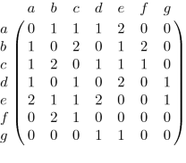
The similarity of communication behaviors of nodes in the network can be used for community detection, and the details of the method will be elaborated in Sect. 4. In this section, we will focus on the calculation method of similarity of communication behavior in a given network. We define the similarity matrix of communication behaviors S = \(\alpha \)W + \(\beta \)A. From the above definition, we can see that with the similarity matrix S, we can directly calculate the node communication behavior similarity \(S_{ij}\), the sum of the node communication behavior similarity \(S_{j}\), and the similarity of communication behavior between node and community \(SC_{ij}\). For simplicity, we apply a specific example to illustrate the proposed method for calculating the similarity of the communication behaviors in a given network. Suppose a network is composed of 7 nodes a, b, c, d, e, f, and g, and times t−1 and t respectively represent the start time and end time of time window Win (t−1, t). The following communication relationships occur within Win (t−1, t) in chronological order: Flow(a,b), Flow(a,c), Flow(c,b), Flow(e,b), Flow(e,c), Flow(c,b), Flow(d,b), Flow(e,f), Flow(d,f), Flow(g,f), and Flow(d,f). Figure 1 presents the resulting network communication relationship graph. Here, the vertices of the graph given in Fig. 1 represent communication nodes, and the edges represent the communication relationships existing between the nodes within Win (t−1, t). The number applied to a given edge represents the weight of the edge, denoting the number of communication interactions between the two constituent nodes of the edge.

Network communication relationship graph of the example illustrating the proposed method for calculating the similarity of the communication behavior of nodes in a network
Based on the above example, the similarity of the communication behavior of nodes is obtained as follows.
-
(1)
Obtain the weight matrix W within Win (t−1, t) from the network communication graph.
It can be seen from the network communication relation graph in Fig. 1 that \(W_{ab}\) is equal to 1 because nodes a and b communicate only once within Win (t−1, t). Accordingly, W is given as follows:
 (4)
(4) -
(2)
Obtain the common communication node number matrix A from the network communication relationship graph.
It can be seen from the network communication relationship graph in Fig. 1 that \(A_{ab}\) is equal to 1 because the number of nodes that nodes a and b communicate with during the interval Win (t−1, t) is 1, and that node is c. Accordingly, A is given as follows:
 (5)
(5) -
(3)
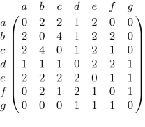
Obtain the communication behavior similarity matrix S from matrices W and A.
The matrix S is obtained according to formula (2) as follows:
$$\mathbf{S} = \alpha \mathbf{W} + \beta \mathbf{A} . $$(6)Here, we let \(W_{ij}\) and \(A_{ij}\) be equally important in calculating \(S_{ij}\) by setting \(\alpha \) and \(\beta \) as 1. Accordingly, we obtain the following matrix S from the network communication relationship graph given in Fig. 1.
 (7)
(7)


4 Community detection algorithm
The proposed community detection algorithm based on the defined node similarity of communication behavior indicator is denoted herein as the CDSCB algorithm. The basic functionality of the algorithm first treats each node in the network as an independent community, and then iteratively merges additional nodes with the highest similarities into each community to obtain the final community division result. The core algorithm is defined below as Algorithm 1. Specifically, a network communication relationship graph g is generated from the input set of edges in row 2 of Algorithm 1, which is then employed to obtain matrices W and A in rows 3 and 4, respectively, based on the input parameter values of \(\alpha \) and \(\beta \). Then, W and A are employed to calculate S in row 5, S and g are employed to calculate the sum of the communication behavior similarity of the nodes SS in row 6, and the nodes are divided into two sets P and Q according to the values of SS in row 7, where the value of SS for each node in P is greater than that in Q. A community is initialized in row 8 with each node in set P to obtain a community set CS, and nodes in set Q are added sequentially to CS in rows 13–18, while all other nodes are added into the temporary set K. Once all the nodes in Q are processed in turn, the algorithm determines whether K is empty in row 19. If K is not empty, then the algorithm returns to row 9 and repeats the steps from rows 13 to 18 until K is empty. Once K is empty, the community obtained with node 1 is merged into the other communities in row 23 according to the similarity between the communities. Finally, the community detection results are returned in row 24.

Figure 2 shows the results of community detection using the CDSCB algorithm for the network in Fig. 1, and Table 1 shows the similarity of the communication behavior of each node in Fig. 1.

Community detection results based on similarity in communication behavior
5 Experimental analysis
5.1 Experimental data
The experimental analyses were conducted based on five public datasets (Karate Club dataset, Dolphins network dataset, Football dataset, Les Misérables’ character relationship dataset,an Email dataset derived from the internal email communication of an European research institute and four real-world IP network datasets (IP-Com1, IP-Com2, IP-Com3, and IP-Com4). The details of these datasets are listed in Tables 2 and 3, respectively. All datasets were based on undirected unweighted networks.
The four IP network datasets described in Table 3 were collected from an actual network environment of an IT company in Beijing, China over different intervals of time on January 17, 2018. The nodes in the dataset are composed of the company’s internal network IP nodes and some external network IP nodes. The edges in the dataset are composed of the communication relationships between these IP nodes, where an edge exists between nodes having a communication relationship, and the weight of the edge is the number of communication interactions between the IP node pairs.
Ground-truth community division results for the above four IP network datasets were obtained by adopting deep packet inspection (DPI) technology to cluster the communication nodes. However, this was not possible for the four public datasets Karate, Dolphins, Football and Les Misérables’ owing to the non-quantitative nature of these four datasets.
5.2 Evaluation metrics and comparison algorithms
The evaluation metrics applied for evaluating the community division performance of the various algorithms are defined as follows.
Modularity (Q) (Newman and Girvan 2004), also denoted as the modular metric, is commonly applied for measuring the results of network community detection. Consider an undirected graph G = (V,E) where V is a set of vertices and E is a set of edges between vertex pairs. \(w_{ij}\) represents the weight of the edge between vertices \(v_{i}\) and \(v_{j}\). \(d_{i}\) represents the sum of the weights of the edges connected to vertex \(v_{i}\). m represents the total number of edges of the graph G. The Modularity (Q) is given by:
where \(c_{i}\) is the community to which vertex \(v_{i}\) belongs, and \(\delta \) is the Kronecker delta function. The value of Q ranges from − 1 to 1, and when the Q value is between 0.3 and 0.7, it indicates a good division of network. This metric is applicable to all datasets considered.
The NMI (Danon et al. 2005) measures the accuracy of community detection by comparing the accuracy of a community division result with the ground-truth result. Define a confusion matrix N, whose rows correspond to the communities really exist in the network, and columns correspond to the communities found by community detection algorithm. \(N_{i,j}\) represents the number of nodes in the existing community i that appear in the j-th detected community, and M is the number of nodes involved in community detection at a certain time. The normalized mutual information I is then:
where C represents the number of communities which really exist in the network and \(\tilde{C}\) represents the number of communities detected by the community detection algorithms. \(N_{i,*}\) represents the sum over the i-th row of N, and \(N_{*,j}\) represents the sum over the j-th column of N. The value of NMI ranges from 0 to 1, and the accuracy of the community detection results increases with increasing NMI. This metric is not applicable to the four public datasets Karate, Dolphins, Football, and Les Misérables due to the unavailability of ground-truth community detection results.
The four state-of-the-art community detection algorithms used for comparison with the method proposed in this paper are given as follows.
The Blondel algorithm proposed by Blondel et al. (2008) in 2008 is a bottom-up algorithm, where each vertex belongs initially to a separate community, and then the vertices move between the communities in an iterative manner to maximize the local contribution of vertices to the overall modularity score. The process continues to the next level when no single movement will increase the modularity score, and each community in the original graph shrinks to a vertex while maintaining the total weight of adjacent edges. This process is repeated until no single movement will increase the modularity score.
The InfoMap algorithm proposed by Rosvall and Bergstrom (2007) in 2007 conducts community division from the perspective of coding. Here, the community structure corresponds to the detection of an optimal secondary coding of the network. The algorithm applies the principle of information compression coding. It first assigns different binary representations to the nodes of the network. Then, a path in the network is expressed in the binary form of the nodes passed by the path, and an objective function is set to the coding length of a random walk path. An optimal secondary coding of the network is then obtained by continuously optimizing the objective function. Accordingly, the goal of community division is accomplished in the process of finding the shortest coding length.
The eigenvector algorithm proposed by Newman (2006) in 2006 belongs to optimization algorithms which employ the modularity matrix to find a division of a network that maximizes the Modularity (Q).
The ALPA algorithm proposed by Han et al. (2017) in 2017 is based on the label propagation algorithm and propagate labels only on the active nodes to reduce computational cost of community detection. It takes into account the historical information and updates its solution through a local label propagation process.
Preliminary analyses of experimental results for the proposed CDSCB algorithm demonstrated that the values of \(\alpha \) and \(\beta \) have no effect on the community detection results when the ratio of \(\alpha \) to \(\beta \) resides within the range 0.1–1.0. Therefore, values of \(\alpha = 0.8\) and \(\beta = 0.2\) were applied for all experiments in this section.
5.3 Comparison of community detection results in terms of modularity
The modularity values of the community detection results obtained by the five algorithms for the four public datasets Karate, Dolphins, Football, and Les Misérables are presented in Fig. 3. As can be seen from the table, the CDSCB and Infomap algorithms achieved higher modularity values for these four datasets than the other algorithms, indicating that their community detection effect was better.

Modularity values obtained for the results of the five community detection algorithms for the four public datasets
Figure 4 presents the community division result obtained by the CDSCB algorithm for the Karate dataset. The result contains two communities, denoted by green nodes and purple nodes, respectively. The algorithm has achieved a good community division result in terms of the general definition of community, where the internal nodes of a community exhibit close connections and the nodes external to the community are sparsely connected.

Community division result obtained by the CDSCB algorithm for the Karate dataset
The existence of ground-truth community division results for the four real-world IP network datasets IP-Com1, IP-Com2, IP-Com3, and IP-Com4 enables a comparison between the modularity values obtained for the ground-truth community division results with the modularity values obtained for the community detection results of the five algorithms for these four datasets, which provides a rigorous and convenient measure of the quality of the community detection results by examining the deviations between the two. The modularity values obtained by the five community detection algorithms and the above-described deviations from the modularity values of the ground-truth community detection results are presented in Table 4.
It can be seen from the table that the CDSCB algorithm obtains community detection results that are very close to the ground-truth community division results, and deviations less than 5% are obtained for all four datasets. It is worth noting that, compared with the CDSCB algorithm, the other four community detection algorithms provide large modularity values when performing community detection on these four datasets, which is a relatively good result for dense networks. However, for IP net-works, higher modularity values do not necessarily match the actual situation, because in most cases, IP networks are generally sparse, and the modularity of these community division results will not be too large.
5.4 Comparison of community detection results in terms of the NMI
The NMI values obtained for the results of the five community discovery algorithms for the Email dataset are presented in Fig. 5. It can be seen from the figure that the CDSCB algorithm obtained the largest NMI value of 0.65 for this dataset, while the Infomap algorithm obtained an NMI value that was slightly smaller. It can also be seen from the figure that the NMI value obtained for the results of the LPA algorithm was 0. Inspection reveals that the LPA algorithm divided all nodes in the Email dataset into a single community, which, by definition, represents an NMI value of 0.

Comparison of the NMI values obtained for the results of the five community discovery algorithms for the Email dataset
The NMI values obtained for the results of the five community detection algorithms for the IP-Com1, IP-Com2, IP-Com3, and IP-Com4 datasets are presented in Fig. 6. As can be seen from the figures, the community detection results of the CDSCB algorithm obtained the largest NMI values of all community detection algorithm results considered, indicating that the CDSCB algorithm is more suitable for conducting community detection in IP networks.

Comparison of the NMI values obtained for the results of the five community detection algorithms for the IP network dataset
It is worth noting that the NMI values obtained by these five community detection algorithms become gradually smaller as the duration of the dataset becomes longer and the number of nodes and edges in the dataset increases. This is because the number of network communities in an IP network and the complexity of community division increase within an increasing number of nodes and edges. At the same time, the occurrence of overlapping communities’ increases. These problems represent serious challenges to community detection algorithms. These results also demonstrate that the accuracy of community detection conducted by algorithms relying on network topology relationships will be greatly affected when sufficient guiding information cannot be obtained from the dataset.
6 Conclusion
This paper addressed the problem of insufficient accuracy of current community detection methods for IP networks by proposing a novel indicator for evaluating the similarity of communication behaviors between IP nodes. This indicator was applied to develop a community detection method, denoted as the CDSCB algorithm. The proposed method mainly takes into account the similarity of communication behavior of the nodes of the same community in the IP network, and uses this feature to cluster the nodes in the network for achieving high-quality community detection. The results of experiments involving both complex public network datasets and real-world IP network datasets demonstrated that the proposed CDSCB algorithm provided superior community detection performance compared to that of four existing state-of-the-art community detection methods in terms of modularity and NMI indicators. In future research, we will seek to improve the method for calculating the similarity of communication behaviors between IP nodes and improve the performance of the community detection method to make it more suitable for application to real-world IP networks with very large numbers of nodes and communication relationships.
References
Ahn YY, Bagrow JP, Lehmann S (2010) Link communities reveal multiscale complexity in networks. Nature 466(7307):761–764
Aiello W, Kalmanek C, McDaniel P, Sen S, Spatscheck O, Van der Merwe J (2005) Analysis of communities of interest in data networks. In: International workshop on passive and active network measurement, Springer, pp 83–96
Baddar SWAH, Merlo A, Migliardi M (2014) Anomaly detection in computer networks: a state-of-the-art review. J Wirel Mob Netw Ubiquitous Comput Dependable Appl 5(4):29–64
Blondel VD, Guillaume JL, Lambiotte R, Lefebvre E (2008) Fast unfolding of communities in large networks. J Stat Mech Theory Exp 10:P10008
Carusi C, Bianchi G (2019) Scientific community detection via bipartite scholar/journal graph co-clustering. J Inform 13(1):354–386
Danon L, Diaz-Guilera A, Duch J, Arenas A (2005) Comparing community structure identification. J Stat Mech Theory Exp 09:P09008
Girvan M, Newman ME (2002) Community structure in social and biological networks. Proc Natl Acad Sci 99(12):7821–7826
Han J, Li W, Zhao L, Su Z, Zou Y, Deng W (2017) Community detection in dynamic networks via adaptive label propagation. PLoS One 12(11):e0188655
Jakalan A, Gong J, Weiwei Z, Su Q (2015) Clustering and profiling ip hosts based on traffic behavior. J Netw 10(2):99
Jakalan A, Gong J, Su Q, Hu X, Abdelgder AM (2016) Social relationship discovery of ip addresses in the managed ip networks by observing traffic at network boundary. Comput Netw 100:12–27
Javed MA, Younis MS, Latif S, Qadir J, Baig A (2018) Community detection in networks: a multidisciplinary review. J Netw Comput Appl 108:87–111
Jiang L, Shi L, Liu L, Yao J, Yousuf MA (2019) User interest community detection on social media using collaborative filtering. In: Wireless networks pp 1–7
Jokar E, Mosleh M (2019) Community detection in social networks based on improved label propagation algorithm and balanced link density. Phys Lett A 383(8):718–727
Karataş A, Şahin S (2018) Application areas of community detection: a review. In: 2018 International congress on big data, deep learning and fighting cyber terrorism (IBIGDELFT), IEEE, pp 65–70
Kelley S, Goldberg M, Magdon-Ismail M, Mertsalov K, Wallace A (2012) Defining and discovering communities in social networks. In Handbook of optimization in complex networks. Springer, New York, pp 139–168
Liang H, Feng DG, Pu-Rui SU, Ying LY, Yi Y (2015) Parallel community detection based worm containment in online social network. Chin J Comput 38(4):846–858
Luo W, Lu N, Ni L, Zhu W, Ding W (2020) Local community detection by the nearest nodes with greater centrality. Inf Sci 517:377–392
Newman ME (2006) Finding community structure in networks using the eigenvectors of matrices. Phys Rev E 74(3):036104
Newman ME, Girvan M (2004) Finding and evaluating community structure in networks. Phys Rev E 69(2):026113
Nguyen NP, Dinh TN, Shen Y, Thai MT (2014) Dynamic social community detection and its applications. PLoS One 9(4):e91431
Pan X, Wu B (2018) Research on criminal gang discovery algorithm based on social networks. Softw Guide 17(12):81–84
Raghavan UN, Albert R, Kumara S (2007) Near linear time algorithm to detect community structures in large-scale networks. Phys Rev E 76(3):036106
Rossetti G, Cazabet R (2018) Community discovery in dynamic networks: a survey. ACM Comput Surv (CSUR) 51(2):1–37
Rosvall M, Bergstrom CT (2007) Maps of information flow reveal community structure in complex networks. arXiv preprint physicssoc-ph/07070609
vanDongen S (2000) A cluster algorithm for graphs. In: Information systems [INS] (R 0010)
Xu K, Wang F, Gu L (2013) Behavior analysis of internet traffic via bipartite graphs and one-mode projections. IEEE/ACM Trans Netw 22(3):931–942
Yang K, Xu Y (2019) An effective method for complex network community detection based on hierarchical splitting. In: Proceedings of the 2019 4th international conference on mathematics and artificial intelligence, pp 10–14
Yang B, Liu D, Liu J (2010) Discovering communities from social networks: methodologies and applications. In Handbook of social network technologies and applications. Springer, New York, pp 331–346
Yang J, McAuley J, Leskovec J (2013) Community detection in networks with node attributes. In: 2013 IEEE 13th international conference on data mining, IEEE, pp 1151–1156
You X, Ma Y, Liu Z (2020) A three-stage algorithm on community detection in social networks. Knowl Based Syst 187:104822
Yu K, Zhang X, Di J, Wu X (2012) Internet traffic identification based on community detection by label propagation. In: 2012 IEEE 2nd international conference on cloud computing and intelligence systems, IEEE, vol 2, pp 786–791
Zhang Y, Wu B, Liu Y, Lv J (2019) Local community detection based on network motifs. Tsinghua Sci Technol 24(6):716–727
Zheng R (2019) A fast community detection algorithm based on clustering coefficient. In: 3rd International conference on mechatronics engineering and information technology (ICMEIT 2019), Atlantis Press
Zhou Z, Amini AA (2019) Analysis of spectral clustering algorithms for community detection: the general bipartite setting. J Mach Learn Res 20:47–1
Author information
Authors and Affiliations
Corresponding author
Additional information
Publisher's Note
Springer Nature remains neutral with regard to jurisdictional claims in published maps and institutional affiliations.
Rights and permissions
Open Access This article is licensed under a Creative Commons Attribution 4.0 International License, which permits use, sharing, adaptation, distribution and reproduction in any medium or format, as long as you give appropriate credit to the original author(s) and the source, provide a link to the Creative Commons licence, and indicate if changes were made. The images or other third party material in this article are included in the article's Creative Commons licence, unless indicated otherwise in a credit line to the material. If material is not included in the article's Creative Commons licence and your intended use is not permitted by statutory regulation or exceeds the permitted use, you will need to obtain permission directly from the copyright holder. To view a copy of this licence, visit http://creativecommons.org/licenses/by/4.0/.
About this article

Cite this article
Zhang, S., Zhang, Y., Zhou, M. et al. Community detection based on similarities of communication behavior in IP networks. J Ambient Intell Human Comput 13, 1451–1461 (2022). https://doi.org/10.1007/s12652-020-02681-w
Received:
Accepted:
Published:
Issue Date:
DOI: https://doi.org/10.1007/s12652-020-02681-w