Evaluating card-based protocols in terms of execution time

Abstract

Card-based cryptography is an attractive and unconventional computation model; it provides secure computing methods using a deck of physical cards. It is noteworthy that a card-based protocol can be easily executed by non-experts such as high school students without the use of any electric device. One of the main goals in this discipline is to develop efficient protocols. The efficiency has been evaluated by the number of required cards, the number of colors, and the average number of protocol trials. Although these evaluation metrics are simple and reasonable, it is difficult to estimate the total number of operations or execution time of protocols based only on these three metrics. Therefore, in this paper, we consider adding other metrics to estimate the execution time of protocols more precisely. Furthermore, we actually evaluate some of the important existing protocols using our new criteria.

1 Introduction

Card-based protocols are unconventional computing methods using a deck of physical cards; their advantage is that they can be executed by humans practically (e.g., [4, 8, 11, 16]). To illustrate this, let us explain how to manipulate Boolean values based on a two-colored deck of cards. Given a black card and a red card  , a Boolean value can be expressed as:

(1)

Following this encoding, for example, two players, Alice and Bob, can each put two cards face down on a table, representing their private bits a and b, respectively:

(2)

Here, we assume that the backs of all cards are indistinguishable and that the fronts or are also indistinguishable if the cards have the same color. We call the left pair of two face-down cards in (2) a commitment to a. Similarly, the right pair of two face-down cards are a commitment to b.

Typically, given two input commitments to $a,b\in \{0,1\}$, as in (2), a card-based protocol should generate a commitment to the value of a predetermined function $f\left( a,b\right)$. For instance, we can get a commitment to $a \wedge b$ without leaking any information about a and b, if we execute an AND protocol:

Table 1 The existing AND protocols (in committed format)

As in Table 1, there are many existing AND protocols (in committed format¹). This table implies that the design of “efficient” protocols is one of the goals of card-based protocols; so far, the efficiency has been evaluated in terms of three metrics: (i) the number of required cards, (ii) the number of colors, and (iii) the average number of required trials. These evaluation metrics are simple and reasonable. However, if we are going to actually execute a card-based protocol, these three metrics are insufficient to accurately estimate the number of operations that need to be done during the protocol and the overall execution time of the protocol.

Therefore, in this paper, we introduce new metrics to evaluate protocol efficiency more precisely. That is, we determine all the operations during a protocol to help analyze the execution time. Furthermore, we actually evaluate all the AND protocols² shown in Table 1, based on our new criteria by counting the number of operations thoroughly. As an application example, we also make a comparison of the AND protocols and discuss which protocol is the most efficient and practical.

The rest of this paper is organized as follows: In Sect. 2, we introduce the AND protocol invented by Stiglic [23] as an example and then give a formalization of the operations in card-based protocols [10]. In Sect. 3, we give new metrics of efficiency, which directly indicate the execution time of a protocol. In Sect. 4, we evaluate the existing AND protocols based on our proposed metrics. In Sect. 5, we conduct a further investigation into evaluation of the execution time. We conclude this study in Sect. 6.

An earlier version of this paper was presented and appeared as a conference paper [7]. The difference is as follows. This paper takes the AND protocol recently proposed by Abe et. al. [1] into account, so that Sect. 3.2.4 along with Fig. 8 has been added and Sect. 4 has been updated. Furthermore, this paper first creates a full version of the KWH-tree [6] of the Crépeau–Kilian AND protocol [3] as Fig. 6 in Sect. 3.2.2 and that of the Niemi–Renvall AND protocol [15] as Fig. 7 in Sect. 3.2.3. In addition, this paper investigates the execution time of rearrangement operations for cards more precisely; Sect. 5 is devoted to this new treatment.

2 Preliminaries: a protocol with operations

In this section, we introduce Stiglic’s AND protocol [23] as an example to demonstrate the possible operations in card-based protocols. It should be noted that card-based protocols are outside the Turing model [10, 12].

As seen in Table 1, Stiglic’s protocol requires a two-colored deck of eight cards and two average trials. Given input commitments to a and b along with four additional cards  , the protocol proceeds as follows:

• 1. Arrange the sequence as:

  

• 2. Apply a random cut to the sequence of eight cards:

  

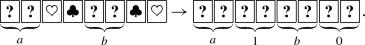
  The term “random cut” means a cyclic shuffle. If we attach numbers to the cards for the sake of convenience:

  

  then a random cut results in one of the following eight sequences (with a probability of $\tfrac{1}{8}$):

  

  Note that a random cut is known to be easily implemented by humans securely via the Hindu cut [25] as shown in Fig. 3.

• 3. Turn over the first two cards (from the left).

  • (a) If the revealed cards are  , we obtain a commitment to $a\wedge b$ as follows:

    

  • (b) If the revealed cards are  , we obtain

    

  • (c) If the revealed cards are or  , turn over the third card.

    • i. If the three face-up cards are  , we have

      

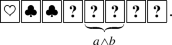
    • ii. If the three face-up cards are  , we have

      

    • iii. If the three face-up cards are or  , turn them over and go back to Step 2.

This is Stiglic’s AND protocol, which we denote by ${\mathcal {P}}_{\mathrm {Sti}}$ hereinafter. A shuffling operation called a random cut is used in Step 2 of $\mathcal {P_\mathrm {Sti}}$. The average number of trials is two, because the probability that Step 3–(c)–iii occurs and we go back to Step 2 is $\frac{1}{2}$.

As seen partially in the description of $\mathcal {P_\mathrm {Sti}}$, the possible operations used in card-based protocols (not just Stiglic’s but others that have not been described thus far) are turning-over, rearrangement, and shuffling operations, which can be formalized as follows [10]. Below, we assume a sequence of d cards $\Gamma = \left( \alpha _1,\alpha _2,\ldots ,\alpha _d\right)$.

• 1. Turning-over operation: (${\textsf {turn}},i$). A $\mathsf {turn}$ operation involves turning over the ith card $\alpha _i$, as shown in Fig. 1. The resulting sequence is

  $$\begin{aligned} \left( \alpha _1,\ldots ,\alpha _{i\!-\!1},\beta _i,\alpha _{i\!+\!1},\ldots ,\alpha _d\right) , \end{aligned}$$

  where $\beta _i$ is obtained by turning over $\alpha _i$.

• 2. Rearrangement operation: (${\textsf {perm}},\pi$). A $\mathsf {perm}$ operation involves the application of a permutation $\pi \in S_d$ (where $S_d$ represents the symmetric group of degree d) to the sequence, as illustrated in Fig. 2. The resulting sequence is

  $$\begin{aligned} \left( \alpha _{\pi ^{-1}\text{(1) }},\alpha _{\pi ^{-1}\text{(2) }},\dots ,\alpha _{\pi ^{-1}\text{( }d\text{) }}\right) . \end{aligned}$$

• 3. Shuffling operation: (${\textsf {shuffle}},\Pi ,{\mathcal {F}}$). A $\mathsf {shuffle}$ operation involves the application of a permutation $\pi \in \Pi$ chosen from a permutation set $\Pi \subseteq \,S_d$ according to a probability distribution ${\mathcal {F}}$. See Fig. 3 again for an example of a shuffle. Note that a set $\Pi$ along with a distribution ${\mathcal {F}}$ specifies a shuffle. We simply write (${\textsf {shuffle}},\Pi$) if ${\mathcal {F}}$ is uniform.

Fig. 1

Turning-over operation

Fig. 2

Rearrangement operation

Fig. 3

Shuffling operation: The Hindu cut

We define

$$\begin{aligned} {\mathsf {R}}{\mathsf {C}}^{\{i_1,i_2,\ldots ,i_\ell \}}\overset{\mathrm {def}}{=}\{\left( i_1 \ i_2 \ \cdots \ i_\ell \right) ^{j}\mid 1\le j \le \ell \}, \end{aligned}$$

for a cyclic permutation ($i_1\,i_2\,\cdots \,i_\ell$) such that $i_1<i_2<\cdots <i_\ell$. Note that the random cut in Stiglic’s protocol can be expressed as (${\textsf {shuffle}},{\mathsf {R}}{\mathsf {C}}^{\{1,2,3,4,5,6,7,8\}}$).

3 New metrics and execution time of protocols

As mentioned in Sect. 2, ${\textsf {turn}}$, ${\textsf {perm}}$, and ${\textsf {shuffle}}$ operations are used in card-based protocols. We need to take these operations into account to analyze the “execution time” of protocols. In other words, the efficiency evaluation metrics shown in Table 1, i.e., the number of required cards, the number of colors, and the average number of trials, are insufficient to estimate the overall execution time.

In Sect. 3.1, we clarify all the operations that need to be considered. In Sect. 3.2, we count the number of occurrences of each operation for every AND protocol. In Sect. 3.3, we provide new metrics to estimate the execution time of protocols.

3.1 Operations to consider

In addition to the three kinds of operations, i.e., ${\textsf {turn}}$, ${\textsf {perm}}$, and ${\textsf {shuffle}}$, introduced in Sect. 2, we define another operation, named ${\textsf {add}}$. The ${\textsf {add}}$ operation involves the addition of a card to the sequence with its face up (in order for players to be able to confirm the color), as shown in Fig. 4. When actually executing a protocol that requires additional cards, this ${\textsf {add}}$ operation is necessary.

Fig. 4

Add operation: adding two cards

Therefore, altogether, the actual execution of a card-based protocol invokes four kinds of operations: ${\textsf {add}}$, ${\textsf {turn}}$, ${\textsf {perm}}$, and ${\textsf {shuffle}}$.

3.2 Analysis of the number of operations in each protocol

In this subsection, we analyze the number of operations in each of the seven existing AND protocols shown in Table 1. To this end, we use the KWH-tree [6] developed by Koch, Walzer, and Härtel, which is a diagram showing the state transition.

Let us take the KWH-tree of ${\mathcal {P}}_{\mathrm {Sti}}$ shown in Fig. 5 as an example to explain the notation of the KWH-tree. Each box is associated with the “visible sequence trace” that means transitions of a sequence of cards visible from the table during the execution of the protocol. In each box, there are sequences of colors and the associated polynomials next to them. A polynomial represents the conditional probability that the current sequence is compatible with the associated sequence of colors (given the visible sequence trace), where $X_{ij}$ denotes the probability that the input is (i, j).

3.2.1 Stiglic’s protocol

We first analyze $\mathcal {P_\mathrm {Sti}}$ in detail. The KWH-tree of $\mathcal {P_\mathrm {Sti}}$ is shown in Fig. 5. This figure enables us to count all the operations appearing in $\mathcal {P_\mathrm {Sti}}$, as follows:

• 1. The number of ${\textsf {add}}$ (adding a card) operations The number of ${\textsf {add}}$ operations in $\mathcal {P_\mathrm {Sti}}$ is four, because we add four cards to execute the protocol.

• 2. The number of ${\textsf {turn}}$(turning over a card) operations Firstly, we execute the ${\textsf {turn}}$ operation four times, because we need to turn over the four added cards after checking their colors. Secondly, we require the ${\textsf {turn}}$ operation twice because of $\left( \mathsf {turn},{\{1,2\}}\right)$ after applying the first random cut. At this time, the probability that or appears and the protocol terminates is $\frac{1}{8}\times 2$. On the other hand, the probability that the protocol terminates by $\left( \mathsf {turn},{\{3\}}\right)$ is $\frac{3}{8}\times \frac{1}{3}\times 2$. If the protocol does not terminate by $\left( \mathsf {turn},{\{3\}}\right)$, we have to turn over the three face-up cards and execute $\left( \mathsf {turn},{\{1,2\}}\right)$ again after applying a random cut. Consequently, the expected number of ${\textsf {turn}}$ operations in $\mathcal {P_\mathrm {Sti}}$ is

  $$\begin{aligned} 4\,+\,{\displaystyle \Sigma _{n=1}^{\infty }}\left( \left( 12n-7\right) \times 1\text{/ }4\times \left( 1\text{/ }2\right) ^{n-1}\right) = 12.5. \end{aligned}$$

• 3. The number of ${\textsf {perm}}$ (rearranging a sequence of cards) operations We use no ${\textsf {perm}}$ operation in $\mathcal {P_\mathrm {Sti}}$, and hence, the number of utilizations of the ${\textsf {perm}}$ operation is 0.

• 4. The number of ${\textsf {shuffle}}$ (shuffling a sequence of cards) operations As seen in the calculation for ${\textsf {turn}}$, the probability that $\mathcal {P_\mathrm {Sti}}$ terminates by $\left( \mathsf {turn},{\{1,2\}}\right)$ is $\frac{1}{4}$. The probability that $\mathcal {P_\mathrm {Sti}}$ terminates by $\left( \mathsf {turn},{\{3\}}\right)$ is $\frac{1}{4}$, and the probability that $\mathcal {P_\mathrm {Sti}}$ does not terminate and gets into a loop is $\frac{1}{2}$. Therefore, the expected number of ${\textsf {shuffle}}$ operations is 2.

Thus, the numbers of ${\textsf {add}}$, ${\textsf {turn}}$, ${\textsf {perm}}$, and ${\textsf {shuffle}}$ operations are 4, 12.5, 0, and 2, respectively. See the line of $\mathcal {P_\mathrm {Sti}}$ in Table 2.

Fig. 5

${\mathcal {P}}_\mathrm {Sti}$’s KWH-tree

3.2.2 Crépeau and Kilian’s protocol

We also create the KWH-tree of $\mathcal {P_\mathrm {CK}}$ (Crépeau and Kilian’s protocol [3]) as shown in Fig. 6, which tells us that the numbers of ${\textsf {add}}$, ${\textsf {turn}}$, ${\textsf {perm}}$, and ${\textsf {shuffle}}$ operations are 6, 21, 1, and 8, respectively. See the line of $\mathcal {P_\mathrm {CK}}$ in Table 2.

Table 2 The number of operations in the practical AND protocols

Fig. 6

${\mathcal {P}}_\mathrm {CK}$’s KWH-tree; this figure is rotated clockwise by $90^\circ$. Note that we use (six) $\mathsf {perm}^*$ in this figure for avoiding the KWH-tree to be complicated; the original ${\mathcal {P}}_\mathrm {CK}$ in [3] does not use them, and we do not count the number of them for Table 2

3.2.3 Niemi and Renvall’s protocol

The KWH-tree of $\mathcal {P_\mathrm {NR}}$ is shown in Fig. 7, from which we can count the numbers of operations as shown in Table 2.

Fig. 7

${\mathcal {P}}_\mathrm {NR}$’s KWH-tree, where $X_{0}=X_{00}+X_{01}+X_{10}$ and $X_{1}=X_{11}$. The above left part makes two copied commitments to a, the above right part makes two copied commitments to b, and the bottom part produces a commitment to $a\wedge b$ from these four commitments

3.2.4 Abe, Hayashi, Mizuki, and Sone’s protocol

The KWH-tree of $\mathcal {P_\mathrm {AHMS}}$ is shown in Fig. 8, from which we can count the numbers of operations as shown in Table 2.

Fig. 8

${\mathcal {P}}_\mathrm {AHMS}$’s KWH-tree [1], where $X_0=X_{00}+X_{01}+X_{10}$ and $X_1=X_{11}$

3.2.5 The others

The KWH-tree of $\mathcal {P_\mathrm {MS}}$ (Mizuki and Sone’s protocol [13]) has been given in some existing literatures (e.g., [6, 12]). Utilizing this KWH-tree, we are able to count each operation in $\mathcal {P_\mathrm {MS}}$. Table 2 summarizes the result.

In addition, we conducted the same calculation for the two KWH protocols [6]. Table 3 shows the number of operations in the protocols. These protocols need shuffles which have non-uniform probability distributions,³ and hence, they need special indistinguishable boxes or envelopes [16] to be implemented. Therefore, we have judged that these two protocols are more time-consuming than the other five protocols. Therefore, in the sequel, we focus on the five protocols in Table 2, which we call “practical” AND protocols.

3.3 Execution time of protocols

In this subsection, we present an expression for the execution time of each protocol based on four metrics. First, we denote the execution time of ${\textsf {add}}$, ${\textsf {turn}}$, ${\textsf {perm}}$, and ${\textsf {shuffle}}$ by ${ {t_\mathrm {add}}}$, ${ {t_\mathrm {turn}}}$, ${ {t_\mathrm {perm}}}$, and ${ {t_\mathrm {shuf}}}$, respectively. In addition, $\mathrm {Time\left( {\mathcal {P}}\right) }$ denotes the overall execution time of a protocol ${\mathcal {P}}$. Then, the execution time of the protocols in Table 2 can be simply expressed as follows:

• 1. Crépeau & Kilian’s protocol ($\mathcal {P_\mathrm {CK}}$): $\mathrm {Time\left( {\mathcal {P}}_\mathrm {CK}\right) } = 6{{ {t_\mathrm {add}}}}+21{{ {t_\mathrm {turn}}}}+{{ {t_\mathrm {perm}}}}+8{{ {t_\mathrm {shuf}}}}$.

• 2. Niemi & Renvall’s protocol ($\mathcal {P_\mathrm {NR}}$): $\mathrm {Time\left( {\mathcal {P}}_\mathrm {NR}\right) } = 8{{ {t_\mathrm {add}}}}+28{{ {t_\mathrm {turn}}}}+2.5{{ {t_\mathrm {perm}}}}+7.5{{ {t_\mathrm {shuf}}}}$.

• 3. Stiglic’s protocol ($\mathcal {P_\mathrm {Sti}}$): $\mathrm {Time\left( {\mathcal {P}}_\mathrm {Sti}\right) } = 4{{ {t_\mathrm {add}}}}+12.5{{ {t_\mathrm {turn}}}}+2{{ {t_\mathrm {shuf}}}}$.

• 4. Mizuki & Sone’s protocol ($\mathcal {P_\mathrm {MS}}$): $\mathrm {Time\left( {\mathcal {P}}_\mathrm {MS}\right) } = 2{{ {t_\mathrm {add}}}}+4{{ {t_\mathrm {turn}}}}+2{{ {t_\mathrm {perm}}}}+{{ {t_\mathrm {shuf}}}}$.

• 5. Abe & Hayashi & Mizuki & Sone’s protocol ($\mathcal {P_\mathrm {AHMS}}$): $\mathrm {Time\left( {\mathcal {P}}_\mathrm {AHMS}\right) } = {{ {t_\mathrm {add}}}}+17{{ {t_\mathrm {turn}}}}+6{{ {t_\mathrm {perm}}}}+7{{ {t_\mathrm {shuf}}}}$.

In the next section, we make a comparison to determine the most efficient and practical protocol.

4 Comparison of the protocols

In this section, we evaluate the efficiency of the five practical AND protocols in Table 2 and discuss which protocol is the most efficient.

4.1 Efficiency comparison based on the execution time

In this subsection, we compare the execution times of the protocols.

First, we compare each coefficient of equation shown in Sect. 3.3 or Table 2. Obviously, we obtain the following inequalities:

$$\begin{aligned}&\mathrm {Time\left( {\mathcal {P}}_\mathrm {Sti}\right) } \,< \mathrm {Time\left( {\mathcal {P}}_\mathrm {CK}\right) }, \\&\mathrm {Time\left( {\mathcal {P}}_\mathrm {Sti}\right) } \, < \mathrm {Time\left( {\mathcal {P}}_\mathrm {NR}\right) }. \end{aligned}$$

Therefore, ${\mathcal {P}}_\mathrm {Sti}$ is superior to ${\mathcal {P}}_\mathrm {CK}$ and ${\mathcal {P}}_\mathrm {NR}$.

Next, we compare ${\mathcal {P}}_\mathrm {Sti}$ with ${\mathcal {P}}_\mathrm {MS}$. At first glance, the coefficients might give us an impression that ${\mathcal {P}}_\mathrm {MS}$ would be better than ${\mathcal {P}}_\mathrm {Sti}$. However, we cannot immediately come to a conclusion because $\mathrm {Time\left( {\mathcal {P}}_\mathrm {MS}\right) }$ has $2{{ {t_\mathrm {perm}}}}$, while $\mathrm {Time\left( {\mathcal {P}}_\mathrm {Sti}\right) }$ has no ${{ {t_\mathrm {perm}}}}$. Therefore, we actually measured the duration of each operation by manipulating real cards. For its experimental method and detailed result, see Appendix A.

Table 3 The number of operations in the KWH protocols [6]

As a result, our measurement provides us the following relationship:

$$\begin{aligned} { {t_\mathrm {add}}}= { {t_\mathrm {turn}}}\ \ \mathrm {and} \ \ 0.1{ {t_\mathrm {perm}}}< { {t_\mathrm {turn}}}. \end{aligned}$$

(3)

Moreover, it is reasonable to assume that

$$\begin{aligned} { {t_\mathrm {perm}}}< { {t_\mathrm {shuf}}}, \end{aligned}$$

because the shuffling operation generally takes more time than the rearrangement operation. From these assumptions, we have $\mathrm {Time\left( {\mathcal {P}}_\mathrm {MS}\right) } < \mathrm {Time\left( {\mathcal {P}}_\mathrm {Sti}\right) }$.

Finally, we compare ${\mathcal {P}}_\mathrm {MS}$ with ${\mathcal {P}}_\mathrm {AHMS}$. Because we have assumed that ${ {t_\mathrm {add}}}={ {t_\mathrm {turn}}}$ as the above, we have $\mathrm {Time\left( {\mathcal {P}}_\mathrm {MS}\right) }<\mathrm {Time\left( {\mathcal {P}}_\mathrm {AHMS}\right) }$.

As a result, we may conclude that ${\mathcal {P}}_\mathrm {MS}$ is the protocol with the least execution time (as long as we admit the above assumptions).

One might think that the execution time of the shuffle used in ${\mathcal {P}}_{\mathrm {Sti}}$ (i.e., a random cut) and the execution time of the shuffle used in ${\mathcal {P}}_{\mathrm {MS}}$ and ${\mathcal {P}}_{\mathrm {AHMS}}$ (i.e., a random bisection cut) are different. We note that the authors in [24] showed that a random bisection cut can be reduced to a random cut if the backsides of all cards are vertically asymmetric such as . Therefore, we may assume that they are the same. Moreover, we measured the execution time of the secure implementation for a random bisection cut proposed in [24], which uses additional tools such as a ball and a rubber band; if we use this implementation, ${\mathcal {P}}_{\mathrm {Sti}}$ is faster (see Sect. 4.3 for the details).

4.2 Impact of execution time of shuffling

In the previous subsection, we assumed that ${ {t_\mathrm {perm}}}< { {t_\mathrm {shuf}}}$ holds. In this subsection, we further investigate how the difference between ${ {t_\mathrm {perm}}}$ and ${ {t_\mathrm {shuf}}}$ affects the overall execution time of a protocol. To this end, we regard ${ {t_\mathrm {shuf}}}$ as a variable and other metrics ${ {t_\mathrm {add}}}$, ${ {t_\mathrm {turn}}}$, and ${ {t_\mathrm {perm}}}$ as constants. Specifically, based on our measurement of the actual execution time, we fix⁴

$$\begin{aligned} {{ {t_\mathrm {add}}}} = {{ {t_\mathrm {turn}}}} = 0.8 \ (\mathrm {sec.}), \ \ {{ {t_\mathrm {perm}}}} = 7{{ {t_\mathrm {turn}}}}. \end{aligned}$$

(4)

Then, we vary the value ${ {t_\mathrm {shuf}}}$ from three seconds to sixty seconds; Fig. 9 shows the result. According to this figure, ${\mathcal {P}}_\mathrm {Sti}$ and ${\mathcal {P}}_\mathrm {MS}$ are considered to be more efficient.

Fig. 9

The total execution time of each protocol for different shuffle times

4.3 Execution time of the secure implementation proposed in [24]

As shown in Table 2, we counted the numbers of the shuffles used in the practical AND protocols in the same way even if they are different. This is because a random bisection cut used in ${\mathcal {P}}_{\mathrm {MS}}$ and ${\mathcal {P}}_{\mathrm {AHMS}}$ can be reduced to the application of the Hindu cut to a sequence of cards if the backsides are vertically asymmetric, as mentioned before. On the other hand, the authors in [24] proposed a secure implementation of a random bisection cut using additional tools such as a ball and rubber band, which does not depend on a pattern of the backsides. Therefore, it is reasonable to consider the case where one uses such an implementation of a random bisection cut in ${\mathcal {P}}_{\mathrm {MS}}$, which might affect our conclusion that ${\mathcal {P}}_{\mathrm {MS}}$ is the fastest one. For this, we measured the execution time of it (denoted by $t_{\mathrm {RBC}}$) by manipulating real tools that are exactly the same ones used in [24]. Its experimental method and result are shown in Appendix A.2.

As a result, we found that $t_{\mathrm {RBC}}>120\,\mathrm {sec}$. Because the authors in [25] showed that it suffices to apply the Hindu cut for 30 s, we derive the following relationship:

$$\begin{aligned} t_{\mathrm {RBC}}>4t_{\mathrm {HC}}, \end{aligned}$$

where $t_{\mathrm {HC}}$ denotes the execution time of applying the Hindu cut. From this, we have $\mathrm {Time\left( {\mathcal {P}}_\mathrm {Sti}\right) }<\mathrm {Time\left( {\mathcal {P}}_\mathrm {MS}\right) }$, and hence, we may conclude that ${\mathcal {P}}_{\mathrm {Sti}}$ is the fastest one (on average) if one uses the above implementation [24].

5 Further investigation of rearrangement operations

In the previous section, we varied the value ${ {t_\mathrm {shuf}}}$, while ${ {t_\mathrm {perm}}}$ is fixed. In this section, we discuss possible necessity of varying the value ${ {t_\mathrm {perm}}}$.

We now enumerate in Table 4 the ${\textsf {perm}}$ operations used in the protocols shown in Table 2. Let us take a look at $\left( \mathsf {perm},{\left( 2\,4\,3\right) }\right)$ used in ${\mathcal {P}}_{\mathrm {MS}}$ as an example. This rearrangement operation can be done by exchanging the second card and the portion consisting the third and fourth cards:

As in this example, any cyclic permutation of the form $\left( i_1\,i_2\,\cdots \,i_\ell \right) ^j$ for some j, $1\le j \le \ell -1$ such that $i_1<i_2<\cdots <i_\ell$ can be done by exchanging two “portions” of cards. Therefore, we can assume that the execution times of the permutations shown in Table 4 except for the ones used in ${\mathcal {P}}_{\mathrm {CK}}$ and ${\mathcal {P}}_{\mathrm {NR}}$ are the same.

In contrast, $\left( \mathsf {perm},{\left( 2\,3\,6\,4\,7\,5\right) }\right)$ used in ${\mathcal {P}}_{\mathrm {CK}}$ and

$$\begin{aligned} \begin{aligned} \pi _1&=\begin{pmatrix} 1 &{} 2 &{} 3 &{} 4 &{} 5 &{} 6 &{} 7 &{} 8 &{} 9 &{} 10 \\ 8 &{} 7 &{} 9 &{} 10 &{} 2 &{} 1 &{} 4 &{} 3 &{} 5 &{} 6 \end{pmatrix},\\ \pi _2&=\begin{pmatrix} 3 &{} 4 &{} 5 &{} 6 &{} 7 &{} 8 &{} 9 &{} 10 &{} 11 &{} 12 \\ 6 &{} 7 &{} 3 &{} 11 &{} 8 &{} 12 &{} 5 &{} 4 &{} 10 &{} 9 \end{pmatrix} \end{aligned} \end{aligned}$$

(5)

(and similar ones) used in ${\mathcal {P}}_{\mathrm {NR}}$ are not such a form. First, $\left( \mathsf {perm},{\left( 2\,3\,6\,4\,7\,5\right) }\right)$ can be illustrated as follows:

To perform this, we move the second card to the third position and the fifth card to the second position and then exchange the portions consisting the third and fourth cards with the portion consisting the sixth and seventh cards. We actually measured the execution time of this move by manipulating real cards. As a result, we found that $\left( \mathsf {perm},{\left( 2\,3\,6\,4\,7\,5\right) }\right)$ takes approximately four times as long as just exchanging two portions.

Table 4 Permutations used in the practical AND protocols, where $\pi _1$ and $\pi _2$ are given in Eq. 5

Remember that $\pi _1$ is one of the six permutations appeared in the left part of ${\mathcal {P}}_{\mathrm {NR}}$’s KWH-tree in Fig. 7. These six permutations are similar: They move the first to fourth cards to the seventh to tenth, the fifth to eighth cards to the first to fourth, and the ninth and tenth cards to the fifth and sixth, respectively. Among the six permutations, $\left( \mathsf {perm},{\pi _1}\right)$ should take the longest time. We also actually measured the execution time of this move. As a result, we found that it takes approximately nine to ten times as long as just exchanging two portions.

Finally, $\pi _2$ is one of the six permutations appeared in the right part of ${\mathcal {P}}_{\mathrm {NR}}$’s KWH-tree. These six permutations are also similar: They move the third and fourth cards to the sixth and seventh, the ninth to tenth cards to the fourth and fifth, and the eleventh to twelfth cards to the ninth to tenth, respectively. They also move the revealed black cards to the third and eighth and the revealed red cards to the eleventh and the twelfth. We also actually measured the execution time of $\left( \mathsf {perm},{\pi _2}\right)$, which should take the longest time among the six permutations. As a result, we found that it takes approximately eleven to twelve times as long as just exchanging two portions.

Therefore, $\mathrm {Time\left( {\mathcal {P}}_\mathrm {CK}\right) }$ and $\mathrm {Time\left( {\mathcal {P}}_\mathrm {NR}\right) }$ could be larger than those in Sect. 3.3. However, even if so, the statement that ${\mathcal {P}}_\mathrm {MS}$ is the protocol with the least execution time (which we concluded in Sect. 4.1) does hold.

The detailed results for measuring the execution time of applying the four permutations can be seen in Appendix A.3.

6 Conclusion

The widely-used efficiency evaluation metrics of card-based protocols do not capture the number of operations fully, and hence, it is difficult to estimate their execution time accurately. Therefore, we considered all kinds of possible operations so that we have four metrics, and focused on counting the number of operations comprehensively to estimate the execution time of protocols. Our new criteria allow us to evaluate the efficiency of protocols. Thus, we were able to compare the execution time of the protocols. Some reasonable assumptions concluded that the Mizuki–Sone AND protocol [13] is the most efficient and practical as an AND protocol in terms of the execution time.

To count the number of operations, we created KWH-trees for $\mathcal {P_\mathrm {CK}}$ and $\mathcal {P_\mathrm {Sti}}$ as shown in Figs. 5 and 6, respectively. This is the first attempt to describe KWH-trees for these previous protocols, and we believe that Figs. 5 and 6 themselves form one of the major contributions of this paper.

Intriguing future work involves applying our new criteria to other existing protocols using different types of cards (e.g., [21, 22]) or those using private operations (e.g., [14, 17,18,19]).

Experimental results

In this appendix, we show our experimental methods and detailed results. A deck of cards used in our experiments is the one shown in Figs. 1 to 4, which was made by the fourth author.

Fig. 10

The tools used in our experiment for measuring the execution time of the secure implementation proposed in [24]; the sequence of six cards, separator, rubber band, curving polystyrene foam ball, tape, and scissors

1.1 Add, turn, and perm

We show how to derive the relationship (3) and (4) shown in Sects. 4.1 and 4.2. This measurement was mainly conducted by the second author, who is familiar with playing cards.

Method. To measure $t_{\mathrm {add}}$ and $t_{\mathrm {turn}}$, we measured the execution time of adding and turning over ten cards five times, respectively. To measure $t_{\mathrm {perm}}$, we measured the execution time of applying all the permutations appeared in ${\mathcal {P}}_{\mathrm {CK}}$, ${\mathcal {P}}_{\mathrm {NR}}$, ${\mathcal {P}}_{\mathrm {Sti}}$, and ${\mathcal {P}}_{\mathrm {MS}}$ (namely six permutations) five times.

Result. Table 5 summarizes the experimental result; $t_{\mathrm {add}}=0.655$, $t_{\mathrm {turn}}=0.803$, and $t_{\mathrm {perm}}=5.889$. Since the difference between $t_{\mathrm {add}}$ and $t_{\mathrm {turn}}$ is relatively small (about 0.15 seconds), we have fixed $t_{\mathrm {add}}=t_{\mathrm {turn}}=0.8$ as in (4).

Table 5 The experimental result of measuring the execution time of adding, turning over, and permuting cards, which was mainly conducted by the second author, who is familiar with playing cards. Since we measured the execution time of adding and turning over ten cards for each time, the values in the rightmost column are the ones in the left of them divided by ten, respectively. For $\mathsf {perm}$, since we measured the execution time of applying six (different) permutations, the value in the rightmost column is the one in the left of it divided by six

Table 6 The experimental result of measuring the execution time of the secure implementation proposed in [24]

Table 7 The experimental result of measuring the four permutations

1.2 Secure implementation using a ball and rubber Band

We show how to derive $t_{\mathrm {RBC}}>120\,\mathrm {sec}$ shown in Sect. 4.3. This evaluation was mainly conducted by the first author, who is an inventor of this implementation.

Method. To measure $t_{\mathrm {RBC}}$, we prepared exactly the same tools in [24] as shown in Fig. 10. We measured the execution time of the following procedure five times:

• 1. Band the two halves of the sequence of six cards using the rubber band and separator.

• 2. Place the banded pile of cards into one half of the curving ball.

• 3. On the half, put the other half and tape them together using the tape and scissors.

• 4. Throw the ball in the air in a spinning manner.

• 5. Remove the tape and rubber band and place the resulting sequence in its original position.

Result. Table 6 summarizes the experimental result. Because it took more than 120 seconds at every time, we have $t_{\mathrm {RBC}}>120\,\mathrm {sec}$.

1.3 Several kinds of permutations

We show experimental method and result for measuring the execution time of the four permutations shown in Sect. 5. This evaluation was mainly conducted by the first author. We measured the execution time of applying each permutation five times. Table 7 summarizes the experimental result.

References

Abe, Y., Hayashi, Y., Mizuki, T., Sone, H.: Five-card AND protocol in committed format using only practical shuffles. In: Proceedings of the 5th ACM on ASIA Public-Key Cryptography Workshop. pp. 3–8. APKC ’18, ACM, New York, NY, USA (2018)
den Boer, B.: More efficient match-making and satisfiability the five card trick. In: Quisquater, J.J., Vandewalle, J. (eds.) Advances in Cryptology – EUROCRYPT ’89. Lecture Notes in Computer Science, vol. 434, pp. 208–217. Springer, Berlin (1990)
Crépeau, C., Kilian, J.: Discreet solitary games. In: Stinson, D.R. (ed.) Advances in Cryptology – CRYPTO’ 93. Lecture Notes in Computer Science, vol. 773, pp. 319–330. Springer, Berlin (1994)
Ishikawa, R., Chida, E., Mizuki, T.: Efficient card-based protocols for generating a hidden random permutation without fixed points. In: Calude, C.S., Dinneen, M.J. (eds.) Unconventional Computation and Natural Computation. Lecture Notes in Computer Science, vol. 9252, pp. 215–226. Springer, Cham (2015)
Koch, A.: The landscape of optimal card-based protocols. Cryptology ePrint Archive, Report 2018/951 (2018). https://eprint.iacr.org/2018/951
Koch, A., Walzer, S., Härtel, K.: Card-based cryptographic protocols using a minimal number of cards. In: Iwata, T., Cheon, J.H. (eds.) Advances in Cryptology—ASIACRYPT 2015. Lecture Notes in Computer Science, vol. 9452, pp. 783–807. Springer, Berlin (2015)
Miyahara, D., Ueda, I., Hayashi, Y., Mizuki, T., Sone, H.: Analyzing execution time of card-based protocols. In: Stepney, S., Verlan, S. (eds.) Unconventional Computation and Natural Computation. Lecture Notes in Computer Science, vol. 10867, pp. 145–158. Springer, Cham (2018)
Mizuki, T., Asiedu, I.K., Sone, H.: Voting with a logarithmic number of cards. In: Mauri, G., Dennunzio, A., Manzoni, L., Porreca, A.E. (eds.) Unconventional Computation and Natural Computation. Lecture Notes in Computer Science, vol. 7956, pp. 162–173. Springer, Berlin (2013)
Mizuki, T., Kumamoto, M., Sone, H.: The five-card trick can be done with four cards. In: Wang, X., Sako, K. (eds.) Advances in Cryptology—ASIACRYPT 2012. Lecture Notes in Computer Science, vol. 7658, pp. 598–606. Springer, Berlin (2012)
Mizuki, T., Shizuya, H.: A formalization of card-based cryptographic protocols via abstract machine. Int. J. Inf. Secur. 13(1), 15–23 (2014)
Mizuki, T., Shizuya, H.: Practical card-based cryptography. In: Ferro, A., Luccio, F., Widmayer, P. (eds.) Fun with Algorithms. Lecture Notes in Computer Science, vol. 8496, pp. 313–324. Springer, Cham (2014)
Mizuki, T., Shizuya, H.: Computational model of card-based cryptographic protocols and its applications. IEICE Transactions on Fundamentals of Electronics, Communications and Computer Sciences E100.A(1), 3–11 (2017)
Mizuki, T., Sone, H.: Six-card secure AND and four-card secure XOR. In: Deng, X., Hopcroft, J.E., Xue, J. (eds.) Frontiers in Algorithmics. Lecture Notes in Computer Science, vol. 5598, pp. 358–369. Springer, Berlin (2009)
Nakai, T., Shirouchi, S., Iwamoto, M., Ohta, K.: Four cards are sufficient for a card-based three-input voting protocol utilizing private permutations. In: Shikata, J. (ed.) Information Theoretic Security. Lecture Notes in Computer Science, vol. 10681, pp. 153–165. Springer, Cham (2017)
Niemi, V., Renvall, A.: Secure multiparty computations without computers. Theor. Comput. Sci. 191(1–2), 173–183 (1998)
Nishimura, A., Nishida, T., Hayashi, Y., Mizuki, T., Sone, H.: Card-based protocols using unequal division shuffles. Soft Comput. (2017). https://doi.org/10.1007/s00500-017-2858-2
Ono, H., Manabe, Y.: Efficient card-based cryptographic protocols for the millionaires’ problem using private input operations. In: 2018 13th Asia Joint Conference on Information Security (AsiaJCIS). pp. 23–28 (2018)
Ono, H., Manabe, Y.: Card-based cryptographic protocols with the minimum number of cards using private operations. In: Zincir-Heywood, N., Bonfante, G., Debbabi, M., Garcia-Alfaro, J. (eds.) Foundations and Practice of Security. Lecture Notes in Computer Science, vol. 11358, pp. 193–207. Springer, Cham (2019)
Ono, H., Manabe, Y.: Card-based cryptographic protocols with the minimum number of rounds using private operations. In: Pérez-Solà, C., Navarro-Arribas, G., Biryukov, A., Garcia-Alfaro, J. (eds.) Data Privacy Management, Cryptocurrencies and Blockchain Technology. Lecture Notes in Computer Science, vol. 11737, pp. 156–173. Springer, Cham (2019)
Ruangwises, S., Itoh, T.: And protocols using only uniform shuffles. In: van Bevern, R., Kucherov, G. (eds.) Computer Science—Theory and Applications. Lecture Notes in Computer Science, vol. 11532, pp. 349–358. Springer, Cham (2019)
Shinagawa, K., Mizuki, T., Schuldt, J.C.N., Nuida, K., Kanayama, N., Nishide, T., Hanaoka, G., Okamoto, E.: Secure computation protocols using polarizing cards. IEICE Trans. 99–A(6), 1122–1131 (2016)
Shinagawa, K., Mizuki, T., Schuldt, J.C., Nuida, K., Kanayama, N., Nishide, T., Hanaoka, G., Okamoto, E.: Card-based protocols using regular polygon cards. IEICE Trans. Fundam. Electron. Commun. Comput. Sci. E100.A(9), 1900–1909 (2017)
Stiglic, A.: Computations with a deck of cards. Theor. Comput. Sci. 259(1–2), 671–678 (2001)
Ueda, I., Miyahara, D., Nishimura, A., Hayashi, Yi, Mizuki, T., Sone, H.: Secure implementations of a random bisection cut. Int. J. Inf. Secur. 19(4), 445–452 (2020). https://doi.org/10.1007/s10207-019-00463-w
Ueda, I., Nishimura, A., Hayashi, Y., Mizuki, T., Sone, H.: How to implement a random bisection cut. In: Martín-Vide, C., Mizuki, T., Vega-Rodríguez, M.A. (eds.) Theory and Practice of Natural Computing. Lecture Notes in Computer Science, vol. 10071, pp. 58–69. Springer, Cham (2016)
Acknowledgements
We thank the anonymous referees, whose comments have helped us to improve the presentation of the paper.
Funding
This work was supported in part by JSPS KAKENHI, Grant Number JP17K00001 and JP19J21153.
Author information
Authors and Affiliations
Corresponding author
Ethics declarations
Conflicts of interest
The authors declare that they have no conflict of interest.
Ethical approval
This article does not contain any new studies with human participants or animals performed by any of the authors.
Additional information
Publisher's Note
Springer Nature remains neutral with regard to jurisdictional claims in published maps and institutional affiliations.