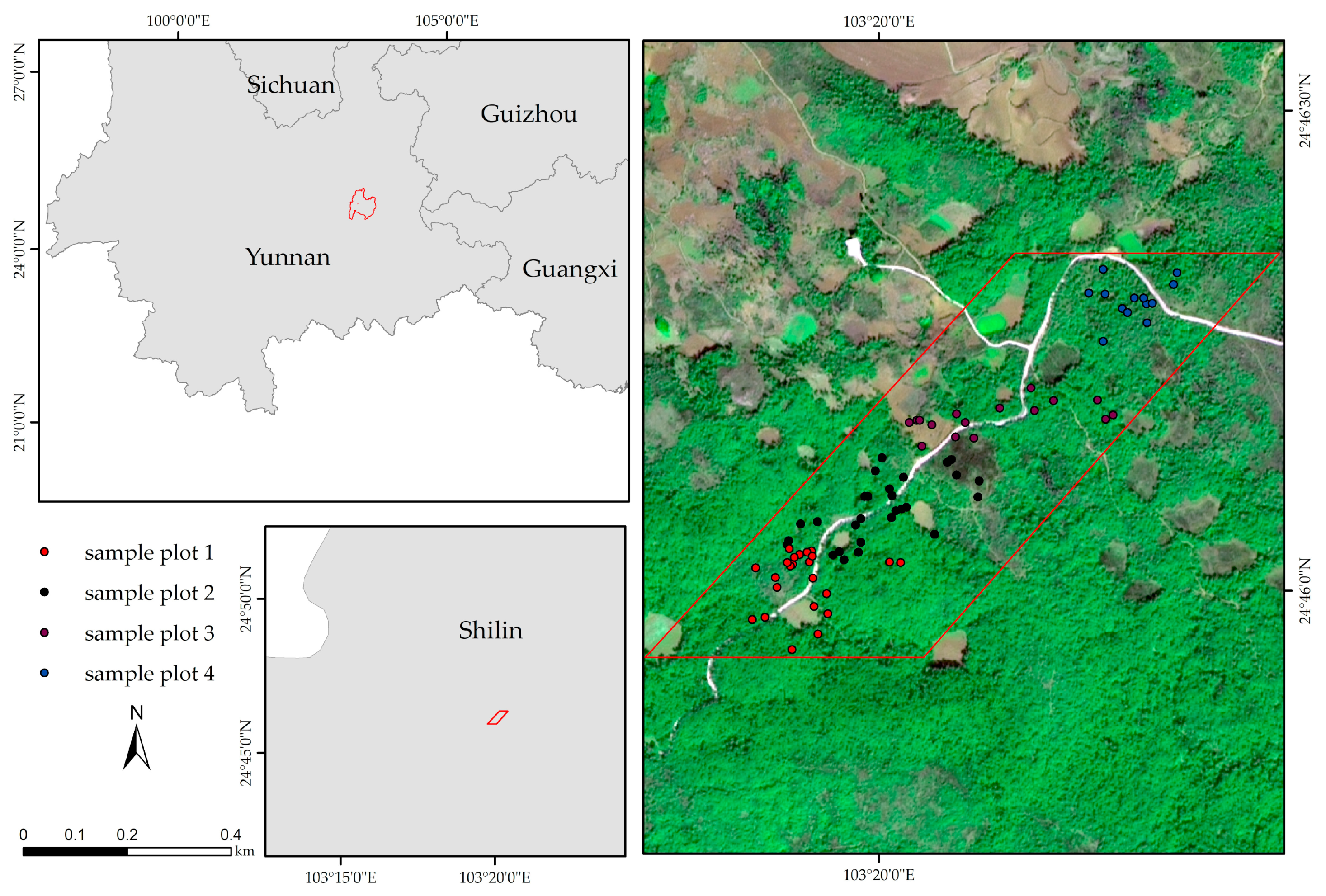
Article

Discriminant Analysis of the Damage Degree Caused by Pine Shoot Beetle to Yunnan Pine Using UAV-Based Hyperspectral Images

1
Research Institute of Resource Insects, Chinese Academy of Forestry; Kunming 650224, China
2
Graduate School, Nanjing Forestry University, Nanjing 210037, China
*
Author to whom correspondence should be addressed.
Forests 2020, 11(12), 1258; https://doi.org/10.3390/f11121258
Submission received: 19 October 2020 / Revised: 23 November 2020 / Accepted: 23 November 2020 / Published: 26 November 2020
(This article belongs to the Special Issue Forestry Applications of Unmanned Aerial Vehicles (UAVs) 2020)

Abstract

:
Due to the increased frequency and intensity of forest damage caused by diseases and pests, effective methods are needed to accurately monitor the damage degree. Unmanned aerial vehicle (UAV)-based hyperspectral imaging is an effective technique for forest health surveying and monitoring. In this study, a framework is proposed for identifying the severity of damage caused by Tomicus spp. (the pine shoot beetle, PSB) to Yunnan pine (Pinus yunnanensis Franch) using UAV-based hyperspectral images. Four sample plots were set up in Shilin, Yunnan Province, China. A total of 80 trees were investigated, and their hyperspectral data were recorded. The spectral data were subjected to a one-way ANOVA. Two sensitive bands and one sensitive parameter were selected using Pearson correlation analysis and stepwise discriminant analysis to establish a diagnostic model of the damage degree. A discriminant rule was established to identify the degree of damage based on the median value between different degrees of damage. The diagnostic model with R690 and R798 as variables had the highest accuracy (R2 = 0.854, RMSE = 0.427), and the test accuracy of the discriminant rule was 87.50%. The results are important for forest damage caused by the PSB.

1. Introduction

Pine shoot beetles (PSBs) [1], Tomicus spp. are important forestry pests that wreak havoc on pine trees and pose a threat to ecological stability. The pests are difficult to find because they can remain hidden in trees for long periods. The damage stage of Tomicus spp. can be divided into two stages, which are the shoot-feeding stage and stem-boring stage. From May to November each year, the adults will migrate to the current year’s shoots after eclosion, which is called the shoot feeding stage. From November to April of the following year, the adults consume the phloem and xylem of the trunk. Then, they mate and lay eggs in the trunk, which is called the stem-boring stage [2,3,4]. PSBs are among the main pests of Yunnan pine (Pinus yunnanensis Franch). Since the first large-scale outbreak in Yunnan, these pests have damaged Yunnan pine in dozens of cities, killing large numbers of pine forests and affecting the forestry industry and local economies [5].
Currently, visual investigation is a common method used for surveying forest diseases and pests, but this method is expensive in terms of manpower and material resources. It is difficult for researchers to navigate deep into the forest hinterland if they are using visual investigation, and the accuracy is often low [6]. Satellite remote sensing technology is also widely used in the study of forest diseases and pests, and vegetation damage in a large area can be observed [7,8]. In recent years, hyperspectral technology has been widely applied to monitor the damage caused by forest diseases and pests, and at present the method is mainly used to observe the spectral changes of infected vegetation, to determine the damage-sensitive bands, to establish monitoring models, and to identify the affected areas. Furthermore, hyperspectral technology can be used to monitor the levels of photosynthetic pigments and nitrogen and water contents of vegetation [9,10,11,12].
A handheld spectrometer is used to measure the vegetation spectrum and to explore the relationship between the spectrum and photosynthetic pigments and plant water content [12]. The changes in chlorophyll of vegetation caused by diseases and pests can be monitored through spectral changes, thereby realizing rapid monitoring [13]. A handheld spectrometer can measure the spectral curves of locally damaged areas of vegetation caused by diseases and pests. Nevertheless, a handheld spectrometer has several drawbacks with regards to monitoring diseases and pests in large areas. Therefore, airborne and spaceborne hyperspectral techniques are increasingly being used in forest disease and pest monitoring.
Hyperspectral imaging is also widely used in plant diseases and insect pests [14,15,16]. It also has applications in forest diseases and pests. For some diseases and pests that cause leaves to wilt and drop, hyperspectral imaging can be used to analyze the relationship between the hyperspectral characteristics and the health status of the vegetation [17,18]. Unmanned aerial vehicle (UAV)-based data and other multiscale hyperspectral data contain a large amount of information on vegetation vitality that can be used to classify the damage degree to vegetation [19] and monitor vegetation health [20].
Hyperspectral data can also be used to study the individual tree or canopy change after being damaged. These data allow for canopy-scale studies of forest health, such as changes in the spectral characteristics of plants after pest and disease infestation [21] or changes in pigment content after forest decline [22]. UAV-based hyperspectral data have also been applied in studies of forest pest monitoring at the individual tree level. The use of UAV-based hyperspectral data in combination with Light Detection and Ranging (LiDAR) data enables effective individual tree level pest monitoring and accurate measurement of the health of individual trees [1].
In this study, visible and partial near-infrared hyperspectral imaging techniques were used to distinguish healthy and damaged Yunnan pine and to identify the severity of PSBs infestation. The results of this study are beneficial for the monitoring of PSBs, and the data provide theoretical support for the use of imaging techniques in monitoring forest diseases and pests. The objectives of this study are to: (1) obtain hyperspectral data of a Yunnan pine canopy, (2) abstract the spectral characteristics of the damaged Yunnan pine, (3) screen sensitive bands and spectral parameters that are most useful for classification, (4) establish diagnostic models to estimate the degree of damage of Yunnan pine affected by PSB, and (5) establish quantitative methods to determine the damage degree.

2. Materials and Methods

2.1. Study Area

The study area is located in the Heilongtan Reservoir forest area, Shilin County, Yunnan Province, China (103°19′53″–103°20′ E, 24°45′59″–24°46′ N). Yunnan pine is the dominant species in the area, characterized by young and middle-aged artificial pure forests that are susceptible to disease and pest infestations. Combined with the historical data from the local forestry office, we identified the Yunnan pines that were damaged by PSBs. These trees were used for the study (Figure 1). According to the “Standard of Forest Pests Occurrence and Disaster (Document Number: LY/T 1681–2006)” issued by the State Forestry Administration, the damage degree of individual Yunnan pine caused by PSB was classified into four levels, as listed in Table 1.

2.2. Data Acquisition

We used a DJI M600 Pro multi-rotor UAV (DJI, Shenzhen, China) equipped with a UHD S185 imaging spectrometer (Cubert GmbH, Ulm, Baden-Württemberg, Germany) to form a UAV-based hyperspectral imaging system. The global position system and inertial measurement unit modules were integrated onto the UAV with a horizontal and vertical position error of approximately 2.0 m and 5.0 m, respectively, with a positioning accuracy of approximately one degree [18,23]. For small-area image analysis, the relative position is more important than the absolute horizontal and vertical position. Therefore, these error ranges are acceptable in small-area forestry surveys. The UHD S185 spectrometer can obtain accurate hyperspectral cube data over the entire field of view instantaneously with its Snapshot imaging technology. The main parameters of the UHD S185 that we used are listed in Table 2. The data acquisition route was planned by DJI Go Pro (DJI, Shenzhen China) based on Google Earth information.
UAV-based data acquisition was carried out in the study areas on 17 November 2019 from 11:00 a.m. to 2:00 p.m. under sunny and windless conditions. Taking into account the actual terrain, the condition of the vegetation in the study area and the study area to be covered, we flew the UAV at an altitude of 100 m above the ground, and the estimated ground sampling distances (GSD) were 0.028 m and 0.56 m for panchromatic and hyperspectral images, respectively. The flight speed was set at 5 m/s. Eight sorties were flown, with the image forward and side overlaps were set to 70% and 60% for each flight, until the entire study area was covered. Before each flight, the UHD S185 scanned the Spectralon® panel (LabSphere, North Sutton, NH, USA) for giving an all-white calibration image with a reflectance of nearly 100% (Figure 2), and then the lens cap was covered and scanned to give an all-black calibration with 0% reflectivity. The above operations were for the correction of hyperspectral cube data. The acquisition area was approximately 0.23 km2. The camera was used to take the photos. Moreover, the position and orientation system (POS) were synchronized to facilitate hyperspectral data correction. When the UAV aerial photography was completed, the aerial photograph was screened to delete the photographs during take-off and landing, and only the photographs of flights within the route plan were retained.
For geometric correction of the hyperspectral data and acquisition of sample trees’ regions of interest (ROIs), a Red-Green-Blue (RGB) orthophoto image of the study area were acquired using DJI Phantom 4 RTK (DJI, Shenzhen China). The flight height was 100 m and the speed was 6 m/s. A total of four sorties were flown. Each flight required calibration photographs before take-off and after landing. DJI Go Pro was also used to plan the acquisition range of the RGB orthophoto image, which corresponded to the acquisition range of the hyperspectral data. However, the acquisition range of the RGB orthophoto image was larger than that of hyperspectral data for subsequent geometric correction of hyperspectral data.

2.3. Data Preprocessing

Rigorous preprocessing was required for the hyperspectral data in order to derive information from the imagery. The preprocessing of hyperspectral data is shown in Figure 3. The mosaic of RGB images was performed with DJI Terra 2.0 (DJI, Shenzhen, China), which allowed quick stitching of photographs captured by DJI Phantom 4 RTK to obtain RGB orthophoto image. The Cubert-Pilot software (Cubert GmbH, Ulm, Baden-Württemberg, Germany) was used to fuse each hyperspectral image with the corresponding panchromatic image acquired at the same time to obtain the fused hyperspectral image. Then, the hyperspectral images were stitched using Agisoft PhotoScan (Agisoft LLC, Saint Petersburg, Russia) with the aid of point cloud data from the panchromatic images to generate hyperspectral orthophoto image. Geometric correction of hyperspectral data was carried out using ENVI’s Image Registration Workflow via the RGB orthophoto image of the study area. Radiometric calibration was directly performed for hyperspectral data after geometric correction, and thus, was provided by the manufacturer. The radiometric calibration method described in Equation (1) (the formula is provided by the manufacturer):
F i = ρ i i G H i m
where ρi is the standard reflection of band i; G is a collection of pixels in a white area of a mask image; m is the number of pixels in the collection; Hi is the spectral radiance of the calibrated image after radiation correction in band i; and Fi is the reflectivity of band i after radiation calibration.

2.4. Spectral Reflectance of Individual Yunnan Pine Canopy

Based on the canopy location information (latitude and longitude) and photographs of each sample tree, the location and size of each canopy was determined on the RGB orthophoto image and the canopy range was plotted (Figure 4) as the ROI. Because the canopy range of a severely damaged tree was difficult to identify, we used the contour of the branches instead of the canopy range. These ROIs were added to the pre-processed hyperspectral image. The average reflectance of the signal ROI was extracted via ENVI (Harris Corporation, Melbourne, FL, USA) as the spectrum of an individual tree for the subsequent analysis.

2.5. First Derivative and Spectral Parameters

The quality of the raw data was poor because the data collection was affected by environmental factors such as soil and light. Therefore, the spectral reflectance curves were smoothed using the Savitzky-Golay (S-G) method [24]. The method eliminates the effects of noise and improves the data quality while preserving as much of the original spectral information as possible. In this study, the original spectral reflectance curve was preprocessed by the 7-point and 3-term S-G method.
The first derivative of the spectral reflectance curve can reflect the position of spectral peaks and troughs very well and plays an extremely important role in the processing of spectral data. Therefore, the first derivative can reflect the slight spectral changes caused by PSB, and thus, it is helpful for monitoring the damage degree. The first derivative [25] was calculated by Equation (2):
ρ ( λ i )   =   [ ρ ( λ i + 1 )     ρ ( λ i   1 ) ] 2 λ ,
where λi is the wavelength at i; ρ ( λ i ) is the spectral value of wavelength λi; and 2△λ is the difference in the wavelength of λi−1 to λi+1, determined by the spectrum sample interval.
The vegetation index is based on the spectral reflectance characteristics of plants, using the spectral reflectance of two or more wavelengths in various combinations and operations to enhance and extract vegetation information, in order to evaluate the growth condition of vegetation by reflecting information related to vegetation physiology or physics through the vegetation index [26]. Many physiological characteristics of Yunnan pine were altered after PSB infestation. The spectral reflectance information of the canopy was also altered. In this study, 28 parameters were selected with reference to the vegetation indices used in previous studies, combining the canopy spectral curves and first derivative features (Table 3).
The spectral curves of each sample tree were obtained after data preprocessing. Pearson correlation analysis of spectral data with the damage degree was performed using the R programming language (AT&T Bell Laboratories, Auckland, New Zealand), and stepwise discriminant analysis was carried out using the Statistical Product and Service Solutions (International Business Machines Corporation, Palo Alto, CA, USA).

2.6. Ground Survey and Individual Yunnan Pine Canopy Survey

A field survey of Yunnan pine in the study area was conducted on 18 November 2019. Four sample plots were set up, and 20 trees were selected for each damage degree. There were a total of 80 sample trees, evenly distributed across the study area. For each sample tree, the number of damaged shoots and total shoots was estimated by visual rough estimation, and the latitude and longitude positions of each tree were recorded. To obtain the relationship between the damaged shoot ratio (DSR) of the canopy (Canopy-DSR) and the DSR of ground survey (Ground-DSR), this study used an M200+Z30 ((DJI, Shenzhen, China) camera to collect canopy data of Yunnan pine. A total of 80 samples were collected with clear pictures of the canopy (Figure 5), which allowed clear visual identification of the damaged shoot. By visual inspection, we obtained the total number of shoots and the number of damaged shoots per canopy. Finally, we calculated the DSR.
The DSR of one individual Yunnan pine can be calculated by Equation (3):
D S R =   n m   ×   100 %
where n is the number of shoots affected by PSB and m is the total number of shoots of an individual Yunnan pine.
Canopy-DSR represents the DSR of one individual Yunnan pine canopy obtained by visual inspection and Ground-DSR represents the DSR of one individual Yunnan pine obtained by ground survey. Each Canopy-DSR has a corresponding Ground-DSR (Table 4).

2.7. Model Building and Accuracy Validation

Seventy percent of the data volume was used for model building and 30% for accuracy validation [32]. A Multivariate Linear Regression (MLR, Equation (4)) model was used to fit the equations [33]:
Y   =   β 0   +   β 1 X 1   +   β 2 X 2   +   β 3 X 3   + +   β n X n   +   ε ,
where Y is the dependent variable; X1 are independent variables; β0 is the intercept; βi is the parameters to be estimated by linear regression analysis; and ε is the additive term of the error.
In this study, the coefficient of determination (R2, Equation (5)), the root-mean-square error (RMSE, Equation (6)), the relative-root-mean-square error (rRMSE, Equation (7)), and the Bias (Equation (8)) were employed as the accuracy verification indicators. The value of R2 is between 0 and 1. If R2 is close to 1, the reference value of the prediction model is high. The smaller the RMSE value was, the more accurate the prediction model was.
R 2 = 1 S S E / S S T ,
R M S E = i = 1 n ( y i y ^ i ) 2 n ,
r R M S E = R M S E y ,
B i a s = i = 1 n ( y ^ i y i ) n ,
where n is the sample size; y i is the measured value at location i; y ^ i is the predicted value at location i; y ¯ is the average value of y; and SST and SSE are the total sum of squares and residual sum of squares, respectively.

3. Results

3.1. The Relationship between Canopy-DSR and Ground-DSR

Pearson correlation analysis was carried out between Canopy-DSR and Ground-DSR [34]. The results showed that Ground-DSR had an extremely significant positive linear correlation with Canopy-DSR, and the Pearson correlation coefficient (PCC, r) was 0.995. Using the proportions of 70% and 30%, 80 sampled trees were divided into a modeling dataset (56 sample trees) and a prediction dataset (24 sample trees). Unitary linear regression was performed to the modeling set with Canopy-DSR as the independent variable and Ground-DSR as the dependent variable; and the equation (y = 0.007 + 1.005x) was obtained (Table 5). We then performed a linear fit between the measured and predicted values, and the results are shown in Figure 6.
As can be seen from Table 5 and Figure 6, Canopy-DSR can be used to fit Ground-DSR, and the accuracy was high (R2 > 0.95, RMSE < 0.05 and Bias < 0.001). Therefore, Ground-DSR can be retrieved by Canopy-DSR to determine the damage degree to Yunnan pine.

3.2. Spectral Characteristics of the Damaged Yunnan Pine Canopy

Figure 7a illustrates the spectral reflectance of the Yunnan pine canopy with different damage degrees, showing the spectral changes. The spectral reflectance curves had significant peaks in the wavelength range of 540–560 nm, and the peak decreased with an increase of the damage degree. The magnitudes were in the order of healthy, mild damage, moderate damage, and severe damage. The reflectance curve showed obvious troughs at 660 to 680 nm, and the value of the troughs increased with the severity of the damage. The reflectance of the healthy Yunnan pine canopy was the lowest, and the reflectance of the other three damage degrees showed no significant differences. At 760 to 946 nm, the reflectance of Yunnan pine canopy decreased as the damage degree increased, with clear differences. After 890 nm, the difference between the different damage degrees decreased and the reflectance values gradually converged.
The first derivative curves of the canopy spectra of Yunnan pine with four damage degrees are shown in Figure 7b. There were significant peaks at 510 to 530 nm, which gradually decreased with the level of damage, but the differences in the values were not significant. There were three troughs and two peaks at 550 to 670 nm, with values at the troughs increasing slightly with increasing damage, but the differences were not significant, and values at the peaks of the four damage degrees were not significantly different. At 700 to 720 nm, there were obvious wave peaks. As the damage degree increased, the peaks decreased significantly, and the position of the peak shifted slightly in the short-wave direction, i.e., there was a “red-edge blue shift.”
The spectral reflectance ratio curves of the healthy/healthy, mild damage/healthy, moderate damage/healthy, and severe damage/healthy ratios can reflect the changes of spectral reflectance of different damage degrees compared to healthy Yunnan pine canopy (Figure 8). From Figure 8, we can see that the reflectance changes of mild damage, moderate damage, and severe damage in Yunnan pine canopies relative to healthy Yunnan pine canopies were roughly similar. At 510 to 570 nm and 695 to 950 nm, the spectral values of mild damage were lower than those of healthy trees. At 500 to 610 nm and 690 to 950 nm, the spectral values of moderate damage were lower than those of healthy trees. At 495 to 645 nm and 685 to 950 nm, the spectral values of severe damage were lower than those of healthy trees. This indicated the range of spectral reflectance below the healthy Yunnan pine canopy gradually increased and above the healthy Yunnan pine canopy gradually decreased as the damage degree increased. From the overall trend, the spectral reflectance of Yunnan pine canopy of the four damage degrees was in order of healthy, mild damage, moderate damage, and severe damage. Therefore, the damage degree can be determined by the spectral reflectance.

3.3. Differential Analysis of Spectra in Yunnan Pine Canopy at Different Damage Degrees

The original spectra, S-G spectra, and first derivatives of the Yunnan pine canopy were analyzed by Pearson correlation with the damage degrees; the bands with the top 10 absolute correlation coefficients (Table 6) were selected for one-way analysis of variance (one-way ANOVA). In the analysis, healthy, mild, moderate, and severe damage were assigned values of 0, 1, 2, and 3, respectively. The results are shown in Figure 9. The bands of the original and S-G spectra were identical, both being 774–810 nm, in the near-infrared band. The band of the original spectrum with the largest correlation coefficient was 798 nm (r = −0.897 **), and those of the S-G spectra were 798 nm and 802 nm, respectively (r = −0.897 **). The bands of the first derivatives with the top 10 correlation coefficients were located around the red-edge region, 698–734 nm, and the band with the largest correlation coefficient was 714 nm (r = −0.922 **). However, the collinearity diagnosis showed that there was severe multicollinearity between these wavelengths, with tolerance approaching 0 and VIF much greater than 10. Therefore, the damage degree estimation model could not be established through these bands. From Figure 9, we could see that the spectral reflectance or first derivative values of the Yunnan pine canopy at different damage degrees were significantly different at these 10 bands (p < 0.05). This means that the damage degree of the Yunnan pine canopy can be differentiated by the values at these wavelengths, and thus, the hazard of an individual Yunnan pine tree can be differentiated.
A discriminant analysis of the damage degree was carried out via the band with the largest correlation coefficient by using Fisher’s discriminant function and leave-one-out cross-validation. The results are shown in Table 7. When using S-G spectral values to distinguish the damage degree, only 798 nm was used for the analysis due to the strong collinearity between 798 nm and 802 nm. The accuracy of all three methods exceeded 70%, with first derivative discrimination being the most effective with an accuracy of 80%.

3.4. Differential Analysis of Hyperspectral Parameters in Yunnan Pine Canopy at Different Damage Degrees

Pearson correlation analysis was performed for hyperspectral parameters and damage degrees. The hyperspectral parameters with the 10 highest absolute correlation coefficients were selected for one-way ANOVA and the results are shown in Figure 10 (Dr: r = −0.924 **, SDr: r = −0.920 **, SDnir: r = 0.806 **, SDy: r = 0.771 **, SDb: r = −0.753 **, Db: r = −0.710 **, SR1: r = −0.704 **, Rg/Rr: r = −0.704 **, (Rg − Rr)/(Rg + Rr): r = −0.699 **, and SR2: r = −0.687 **). There were significant differences in the four damage degrees of Dr, SDr, SDnir, and SDy (p < 0.05). Therefore, the damage degree of Yunnan pine canopy can be distinguished by these hyperspectral parameters. There were no significant differences in SDb or Db between healthy and mild damage, but these two damage degrees were significantly different from the other two. The values of (Rg − Rr)/(Rg + Rr), SR1, Rg/Rr, and SR2 showed no significant difference between mild damage and moderate damage, but these two damage degrees were significantly different from the other two damage degrees. Although some of the 10 hyperspectral parameters could not provide a good discrimination between all four damage degrees, they were able to distinguish severe damage from other degrees.

3.5. Screening of the Damage Degree-Sensitive Variables in Yunnan Pine Canopy

The original spectra (506–602 nm and 690–946 nm, 90 bands), S-G spectra (506–602 nm and 690–946 nm, 90 bands), first derivative values (498–546 nm, 554–618 nm, 626–662 nm, 670–758 nm, 802–830 nm, and 846–946 nm, for a total of 97 bands), and hyperspectral parameters (Dr, SDr, SDnir, SDy, SDb, Db, SR1, Rg/Rr, (Rg − Rr)/(Rg + Rr), SR2, NDVI1, NDVI2, NDVI705, Rg, SDnir/SDb, (SD − SDY)/(SDr + SDy), PRI, Dy, (SDnir − SDb)/(SDnir + SDb), (SDr + SDb), and SDr/SDb, for a total of 21 spectral parameters) of the Yunnan pine canopy, which were significantly correlated with the damage degree, were subjected to stepwise discriminant analysis using Fisher’s discriminant function and Wilks’s Lambda classification method. In the analysis, variables were introduced or eliminated through corresponding statistical tests. In the final discriminant function, only a small number of variables with high discriminative power were retained, while the variables with the lowest discriminative power were eliminated [35]. The results of the stepwise discriminant analysis are shown in Table 8. The sensitive bands of the original spectra were 690 nm and 798 nm, denoted as R690 and R798, respectively. The sensitive bands of S-G were 690 nm and 802 nm, denoted as RS-G690 and RS-G802. The sensitive bands of the first derivative were 650 nm and 714 nm, denoted as D650 and D714. The sensitive parameter was Dr.
The leave-one-out cross-validation was applied to the accuracy test; the results are shown in Table 9. The modeling accuracy of all four spectral treatments exceeded 80%, with the highest accuracy of 86.30% for hyperspectral parameters. The first derivative had the highest cross-validation accuracy of 85.00%. According to the modeling accuracy and cross-validation results, the first derivatives were the best discriminated and the S-G spectra were the worst discriminated. The reason for this result may be that the average spectra of the Yunnan pine canopy was used for analysis in this study. The influences of the atmospheric environment, soil, and temperature on the spectral curve were balanced, and the noise level of the curves were small. On this basis, S-G filtering may cause some of the original information of the spectral curve to be lost, which may result in the lowest discriminative accuracy.

3.6. Modeling the Damage Degree of Yunnan Pine Canopy

Based on the screened original spectra, S-G spectra, first-order derivative sensitive bands and hyperspectral sensitive parameters, MLR models were constructed. Moreover, diagnostic model accuracy was tested via R2, RMSE, rRMSE, and Bias.
R690 and R798, RS-G690 and RS-G802, D650 and D714, and Dr were used to establish MLR models based on the modeling dataset, respectively. The prediction dataset was used for accuracy validation of the models (Table 10). The results showed that the original spectral model fitted best with R2, RMSE and Bias of 0.864, 0.416, and −0.068, respectively. The S-G spectral model gave the best prediction with R2, RMSE and Bias of 0.827, 0.465, and −0.067, respectively. The measured values were fitted linearly to the predicted values, and the results are shown in Figure 11, with R2 exceeding 0.8 for all four methods. There were no significant differences among the four models, and all models could better predict the damage degree caused by PSB to Yunnan pine.

3.7. Quantitative Discriminant Rules of the Damage Degree of the Yunnan Pine Canopy

The quantification discriminant rules of the damage degree were established by the diagnostic model. First, the diagnostic model was used to calculate predicted values of the damage degree for the modeling dataset. Then, the average of the predicted values for each damage degree was calculated. The averages of the predicted values of the two damage degrees were used to calculate the median value between these two damage degrees, and this was used as the threshold to establish the discriminant rule. Finally, the damage degree of the prediction dataset was determined by the rule to verify the accuracy of the discriminant rule. The discriminant rules are shown in Table 11, and the accuracy test results are shown in Table 12. The discriminant rule based on the original spectra had the highest test accuracy of 87.50%; however, the first derivative was the lowest at 79.17%. This rule had the best discrimination for healthy Yunnan pine canopy and the worst discrimination for severe damaged Yunnan pine canopy. Nevertheless, healthy trees could be separated from damaged trees according to this rule.

4. Discussion

Forest tree mortality is the result of multiple factors, making it difficult to predict and discern the causes of mortality [36]. In recent years, hyperspectral remote sensing has been widely applied in field of agriculture and forestry to rapidly obtain effective information concerning vegetation and crops. In our study, Yunnan pine defoliation and mortality were mainly related to PSB. Thus, this study focused on the spectral characteristics, sensitive variables, and discriminant rules for the Yunnan pine canopy after damage by the PSB. Using UAV-based hyperspectral imaging, we developed diagnostic models and discriminant rules for Yunnan pine following damage by PSB, highlighting the application of UAV tools in forest pest management and monitoring and early warning.

4.1. Spectral Characteristics of Damaged Yunnan Pine

In recent decades, a large number of Yunnan pine forests have killed by PSB, which affected the ecological stability and economic outputs of forests [37]. In the study area, PSB has been identified as the most serious forest pest of Yunnan pine. Forest trees affected by pests exhibit specific symptoms, such as yellowing and reddening of leaves, an increased proportion of withering and defoliated trees, a decrease in leaf photosynthetic efficiency, and sudden death [38]. The damage degree was determined by Ground-DSR, but only the vegetation canopy could be observed using satellite and UAV remote sensing. Therefore, we established a relationship between Ground-DSR and Canopy-DSR to determine the damage degree by Canopy-DSR. By analyzing the spectral data, we found that the spectra of damaged Yunnan pine had obvious changes in the green peak (510–560 nm), red valley (640–680 nm), red-edge region (680–740 nm), and near-infrared bands (740–950 nm), consistent with previous studies on the spectral responses of damaged vegetation [6,21,39]. Such spectral changes in leaves and tree canopies indicate that remote sensing could be useful for the monitoring of forest diseases and pests [40].

4.2. Sensitive Band and Parameter Screening

The development of hyperspectral technology has brought new vitality to the monitoring of forest tree diseases and pests. The using of hyperspectral data increases the amount of data storage and transmission as well as the rich spectral information, but it also causes some problems. The whole data processing is tedious and time-consuming because of a large amount of data noise and data redundancy [18]. These shortcomings bring obstacles to the popularization and application of hyperspectral technology. Hence, it is very important to streamline data and improve data processing efficiency. New indicators are formed by the combination of different original bands or function transformation, and sensitive bands are selected by statistical analysis or other methods according to the spectral differences of different monitoring targets [41,42,43]. In recent years, several new methods have emerged for the selection of hyperspectral bands or feature extraction [44], such as the screening of sensitive bands through principal component analysis, the successive projection algorithm, or other algorithms [44,45,46,47].
In this study, Pearson correlation analysis and stepwise discriminant analysis were used to screen sensitive bands and spectral parameters in the spectrum of damaged Yunnan pine. All selected bands were located in red and near-infrared regions, and the parameter (Dr) was also related to the red-edge position. These results are consistent with the characteristics of the spectral changes of damaged Yunnan pine. These bands and parameters were used to establish diagnostic models for the damage degree, with all R2 being greater than 0.8, allowing monitoring of the damage caused by the PSB. Thus, the optimal band and parameter selection method were verified as suitable for the sensitive variable selection of defoliation and yellowing of Yunnan pine needles and can be applied to other pine stands.

4.3. Quantitative Discriminant Rule for the Damage Degree

When establishing the model, we assigned different values to the damage degrees, so it is necessary to establish quantitative discriminant rules to determine the prediction results of the model. The averages of the predicted values of the two different damage degrees were used to calculate the median value between these two damage degrees. Then, the median value was used as the threshold to establish the discriminant rule, and the discriminant accuracy of the degrees of damage reached 87.50%. The rule was most effective in identifying healthy Yunnan pine trees and could distinguish healthy Yunnan pine trees from damaged trees. This discriminant rule can also be applied to the monitoring of other diseases and pests. The method of establishing the discriminant rule based on the median value between two different classes as the threshold is simple to implement and it is effective in discriminating the damaged tree.

4.4. Monitoring Infestation by Tomicus spp.

With the development of remote sensing technology, more and more studies focus on the use of hyperspectral technology for vegetation health and forest management, especially UAV-based hyperspectral imaging for high-resolution and low-cost monitoring of forest pests [1,17,18,19]. In addition, hyperspectral sensors are capable of identifying subtle spectral changes. In the study of defoliation of forest vegetation during the Dendrolimus tabulaeformis Tsai et Liu disaster outbreak, the sensitive spectral bands for defoliation rates were located in the green bands and near the red-edge region [18]. Furthermore, in another study of the damage caused by the European spruce bark beetle, it was found that the wavelengths closely related to the different damage classes were in the red and near-infrared bands [19]. In this study, we found that the sensitive bands for the damage degree caused by PSB were located near the red-edge region and in the near-infrared region. It is worth noting from these studies that the red-edge position and the near-infrared band are very sensitive to forest pests. In addition, the red-edge indices are important for the monitoring of forest disease and pest [17]. This has also been confirmed in our study. The spectral characteristic and discriminant analysis of single damaged trees by UAV-based hyperspectral technology will lay the foundation for low-cost, high- resolution monitoring of forest diseases and pests in large areas.
This study aimed to establish a framework to assess the damage degree to Yunnan pine affected by PSB as follows: (1) the selection of an optimal spectral pretreatment method and the establishment of a diagnostic model and quantitative discriminant rule using sensitive bands based on Pearson correlation analysis and stepwise discriminant analysis or (2) the establishment of a diagnostic model and quantitative discriminant rule using sensitive parameters based on the band combination of the spectrum. Although the framework might not be the best, it is superior to visual investigation in identifying the damage degree caused by PSB. In addition, it is both simple and efficient to implement. The highest discriminant accuracy of this framework for determining the damage degree caused by PSB reached 87.50% with only one or two variables. This result can be combined with multi-spectral satellite remote sensing or other effective methods for large-scale monitoring and accurate identification of damage caused by forest diseases and pests in the future.

4.5. Outlook

The monitoring framework for the damage degree caused by PSB is composed of some simple methods. We drew the tree canopy ROIs manually to extract the spectra. This process involves human participation, which may lead to a reduction in the identification accuracy, and it is not fully applicable to the identification of forest damage at the canopy level. Therefore, in follow-up research, an algorithm can be used to identify the tree canopy according to the textural features. Furthermore, LiDAR can be used to detect a single tree and obtain the tree canopy, which can be combined with UAV-based hyperspectral data for forest disease and pest monitoring [1]. The three-dimensional structure information of a single tree can be obtained according to the LiDAR data, which is also helpful for the monitoring of forest diseases and pests. Furthermore, LiDAR can also be used to monitor insect behavior [48]. Pearson correlation analysis and stepwise discriminant analysis were adopted in the screening of sensitive bands and parameters; these are simple methods. In the future, different algorithms can be used to acquire sensitive bands and parameters to improve the monitoring accuracy.

5. Conclusions

This study proposed a low-cost and miniaturized hyperspectral image data analysis system based on UAV remote sensing. Our study shows the potential of UAV-based hyperspectral remote sensing technology for forest disease and pest monitoring. This technology can be used to distinguish the anomalous reflectance characteristics of trees in small areas. Pearson correlation analysis and stepwise discriminant analysis were used to analyze the damage of Yunnan pine caused by PSB in order to obtain the sensitive bands and spectral parameters. First, the relationship between Ground-DSR and Canopy-DSR was verified, and it was found that there was a highly significant positive correlation and a strong linear relationship between the two indexes. We extracted the canopy spectra through the hand-drawn ROIs to analyze the spectral characteristics of damaged Yunnan pine. Then, Pearson correlation analysis and stepwise discriminant analysis were used to select sensitive bands and spectral parameters. Based on these sensitive variables, diagnostic models of the damage degree were established, and the quantitative discriminant rule was established using the median value as a threshold. The results showed that the diagnostic model with R690 and R798 as parameters was able to determine the damage degree of Yunnan pine using only two variables, and the test accuracy of the discriminant rule based on this model was the highest: 87.50%. This study established a simple framework to effectively identify the damage caused by PSB. In the future, we expect that the framework can be further improved to realize automatic identification and monitoring of the damage caused by PSB, combining LiDAR data, hyperspectral data, and satellite remote sensing data to achieve large-scale monitoring of PSB damage.

Author Contributions

Conceptualization, L.S.; Formal analysis, M.L.; Funding acquisition, Z.Z. and L.S.; Investigation, M.L., Z.Z., X.L. and Y.M.; Methodology, M.L.; Resources, L.S.; Visualization, M.L. and J.Y.; Writing—original draft, M.L.; Writing—review and editing, M.L. and T.D. All authors have read and agreed to the published version of the manuscript.

Funding

This work was supported financially by the National Key Research and Development Project of China (2018YFD0600201-4).

Conflicts of Interest

The authors declare no conflict of interest.

Abbreviations

The following abbreviations are used in this manuscript:
Canopy-DSRdamaged shoot ratio of the canopy
DSRdamaged shoot ratio
ENVIEnvironment for Visualizing Images
Ground-DSRdamaged shoot ratio of ground survey
GSDground sampling distances
LiDARLight Detection and Ranging
MLRMultivariate Linear Regression
NDVINormalized Difference Vegetation Index
NDVI705Red Edge Normalized Difference Vegetation Index
one-way ANOVAone-way analysis of variance
POSposition and orientation system
PRIPhotochemical Reflectance Index
PSBpine shoot beetle
RGBRed-Green-Blue
ROIregion of interest
S-GSavitzky-Golay
SRSimple Ratio Index
UAVUnmanned Aerial Vehicle
VIFVariance Inflation Factor

References

  1. Lin, Q.N.; Huang, H.G.; Wang, J.X.; Huang, K.; Liu, Y.Y. Detection of Pine Shoot Beetle (PSB) Stress on Pine Forests at Individual Tree Level using UAV-Based Hyperspectral Imagery and Lidar. Remote Sens. 2019, 11, 2540. [Google Scholar] [CrossRef] [Green Version]
  2. Ye, H.; Dang, C.L. Study on the harmful behavior of Tomicus piniperda on Pinus yunnanensis. J. Yunnan Univ. 1986, 8, 218–222. [Google Scholar]
  3. Byers, J.A. Simulation of the mate-finding behaviour of pine shoot beetles, Tomicus piniperda. Anim. Behav. 1991, 41, 649–660. [Google Scholar] [CrossRef]
  4. Yu, L.F.; Huang, J.X.; Zong, S.X.; Huang, H.G.; Luo, Y.Q. Detecting Shoot Beetle Damage on Yunnan Pine Using Landsat Time-Series Data. Forests 2018, 9, 39. [Google Scholar] [CrossRef] [Green Version]
  5. Ye, H. Occurrence, distribution and damages of Tomicus piniperda in Yunnan, southwestern China. J. Yunnan Univ. 1998, 20, 3–5. [Google Scholar]
  6. Huang, L.X.; Yang, L.; Meng, L.W.; Wang, J.Y.; Li, S.J.; Fu, X.P.; Du, X.Q.; Wu, D. Potential of Visible and Near-Infrared Hyperspectral Imaging for Detection of Diaphania pyloalis Larvae and Damage on Mulberry Leaves. Sensors 2018, 18, 2077. [Google Scholar] [CrossRef] [PubMed] [Green Version]
  7. Trujillo-Toro, J.; Navarro-Cerrillo, R.M. Analysis of Site-dependent Pinus halepensis Mill. Defoliation Caused by ‘Candidatus Phytoplasma pini’ through Shape Selection in Landsat Time Series. Remote Sens. 2019, 11, 1868. [Google Scholar] [CrossRef] [Green Version]
  8. Balazy, R.; Hycza, T.; Kamińska, A.; Osińska-Skotak, K. Factors Affecting the Health Condition of Spruce Forests in Central European Mountains-Study Based on Multitemporal RapidEye Satellite Images. Forests 2019, 10, 943. [Google Scholar] [CrossRef] [Green Version]
  9. Bach, H.; Mauser, W. Atmospheric correction of hyperspectral data in terms of the determination of plant parameters. Proc. SPIE Int. Soc. Opt. Eng. 1994. [Google Scholar] [CrossRef]
  10. Pea, M.A.; Altmann, S.H. Use of satellite-derived hyperspectral indices to identify stress symptoms in an Austrocedrus chilensis forest infested by the aphid Cinara cupressi. Int. J. Pest Manag. 2009, 55, 197–206. [Google Scholar] [CrossRef]
  11. Yuan, Y.; Hu, X. Random Forest and Objected-Based Classification for Forest Pest Extraction from UAV Aerial Imagery. Int. Arch. Photogramm. 2016, 41, 1093–1098. [Google Scholar] [CrossRef]
  12. Wang, J.Q.; Wu, W.M.; Wang, T.W.; Cai, C.F. Estimation of leaf chlorophyll content and density in Populus euphratica based on hyperspectral characteristic variables. Spectrosc. Lett. 2018, 51, 485–495. [Google Scholar] [CrossRef]
  13. Ju, Y.W.; Pan, J.; Zhang, H.; Wang, X.T. Detection of Bursaphelenchus xylophilus infection in Pinus massoniana from hyperspectral data. Nematology 2014, 16, 1197–1207. [Google Scholar] [CrossRef]
  14. Xie, C.Q.; Yang, C.; He, Y. Hyperspectral imaging for classification of healthy and gray mold diseased tomato leaves with different infection severities. Comput. Electron. Agric. 2017, 135, 154–162. [Google Scholar] [CrossRef]
  15. Kong, W.; Zhang, C.; Huang, W.; Liu, F.; He, Y. Application of hyperspectral imaging to detect Sclerotinia sclerotiorum on oilseed rape stems. Sensors 2018, 18, 123. [Google Scholar] [CrossRef] [PubMed] [Green Version]
  16. Ma, Y.; Huang, M.; Yang, B.; Zhu, Q. Automatic threshold method and optimal wavelength selection for insect-damaged vegetable soybean detection using hyperspectral images. Comput. Electron. Agric. 2014, 106, 102–110. [Google Scholar] [CrossRef]
  17. Coops, N.; Stanford, M.; Old, K.; Dudzinski, M. Assessment of Dothistroma Needle Blight of Pinus radiata Using Airborne Hyperspectral Imagery. Phytopathology 2003, 93, 1524–1532. [Google Scholar] [CrossRef] [Green Version]
  18. Zhang, N.; Zhang, X.L.; Yang, G.J.; Zhu, C.H.; Huo, L.N.; Feng, H.K. Assessment of defoliation during the Dendrolimus tabulaeformis Tsai et Liu disaster outbreak using UAV-based hyperspectral images. Remote Sens. Environ. 2018, 217, 323–339. [Google Scholar] [CrossRef]
  19. Näsi, R.; Honkavaara, E.; Lyytikäinen-Saarenmaa, P.; Blomqvist, M.; Litkey, P.; Hakala, T.; Viljanen, N.; Kantola, T.; Tanhuanpää, T.; Holopainen, M. Using UAV-Based Photogrammetry and Hyperspectral Imaging for Mapping Bark Beetle Damage at Tree-Level. Remote Sens. 2015, 7, 15467–15493. [Google Scholar] [CrossRef] [Green Version]
  20. Lausch, A.; Heurich, M.; Gordalla, D.; Dobner, H. Forecasting potential bark beetle outbreaks based on spruce forest vitality using hyperspectral remote-sensing techniques at different scales. Forest Ecol. Manag. 2013, 308, 76–89. [Google Scholar] [CrossRef]
  21. Meiforth, J.J.; Buddenbaum, H.; Hill, J.; Shepherd, J. Monitoring of Canopy Stress Symptoms in New Zealand Kauri Trees Analysed with AISA Hyperspectral Data. Remote Sens. 2020, 12, 926. [Google Scholar] [CrossRef] [Green Version]
  22. Zarco-Tejada, P.J.; Hornero, A.; Beck, P.S.A.; Kattenborn, T.; Kempeneers, P.; Hernández-Clemente, R. Chlorophyll content estimation in an open-canopy conifer forest with Sentinel-2A and hyperspectral imagery in the context of forest decline. Remote Sens. Environ. 2019, 223, 320–335. [Google Scholar] [CrossRef]
  23. Yang, G.J.; Li, C.C.; Wang, Y.J.; Yuan, H.H.; Feng, H.K.; Xu, B.; Yang, X.D. The DOM generation and precise radiometric calibration of a UAV-mounted miniature snapshot hyperspectral imager. Remote Sens. 2017, 9, 642. [Google Scholar] [CrossRef] [Green Version]
  24. Savitzky, A.; Golay, M.J.E. Smoothing and Differentiation of Data by Simplified Least Squares Procedures. Anal. Chem. 1964, 36, 1627–1639. [Google Scholar] [CrossRef]
  25. Xu, Z.H.; Liu, J.; Yu, K.Y.; Gong, C.H.; Xie, W.J.; Tang, M.Y.; La, R.W.; Li, Z.L. Spectral Features Analysis of Pinus massoniana with Pest of Dendrolimus punctatus Walker and Levels Detection. Spectrosc. Spect. Anal. 2013, 33, 428–433. [Google Scholar] [CrossRef]
  26. Merzlyak, M.N.; Gitelson, A.A.; Chivkunova, O.B.; Rakitin, V.Y. Non-destructive optical detection of pigment changes during leaf senescence and fruit ripening. Physiol. Plant. 2010, 106, 135–141. [Google Scholar] [CrossRef] [Green Version]
  27. Liu, M.Y.; Shi, L.; Ma, Y.Q.; Zhang, Z.H.; Liu, X.L.; Yao, J.; Du, T. Correlation Analysis of Different Hazard Periods of Tomicus spp. Based on Hyperspectral Features and Photosynthetic Parameters. For. Res. 2020, 33, 118–127. [Google Scholar] [CrossRef]
  28. Yuan, L.; Zhang, J.C.; Zhao, J.L.; Huang, W.J. Differentiation of Yellow Rust and Powdery Mildew in Winter Wheat and Retrieving of Disease Severity Based on Leaf Level Spectral Analysis. Spectrosc. Spect. Anal. 2013, 33, 1608–1614. [Google Scholar] [CrossRef]
  29. Das, P.K.; Laxman, B.; Rao, S.V.C.K.; Seshasai, M.V.R.; Dadhwal, V.K. Monitoring of bacterial leaf blight in rice using ground-based hyperspectral and LISS IV satellite data in Kurnool, Andhra Pradesh, India. Int. J. Pest Manag. 2015, 61, 359–368. [Google Scholar] [CrossRef]
  30. Gong, P.; Pu, R.; Heald, R.C. Analysis of in situ hyperspectral data for nutrient estimation of giant sequoia. Int. J. Remote Sens. 2002, 23, 1827–1850. [Google Scholar] [CrossRef]
  31. Wu, T.; Ni, S.X.; Li, Y.M.; Zhou, X.X.; Chen, J. Monitoring of the Damage Intensity Extent by Oriental Migratory Locust Using of Hyper-spectra Data Measured at Ground Surface. Int. J. Remote Sens. 2007, 11, 103–108. [Google Scholar]
  32. Nansen, C.; Elliott, N. Remote Sensing and Reflectance Profiling in Entomology. Annu. Rev. Entomol. 2016, 61, 139–158. [Google Scholar] [CrossRef] [PubMed] [Green Version]
  33. Aparicio, T.; Villanua, I. Multivariate linear regression model. In Computer-Aided Introduction to Econometrics; Springer: Berlin/Heidelberg, Germany, 2003; pp. 45–120. [Google Scholar] [CrossRef]
  34. Pearson, K. Determination of the Coefficient of Correlation. Science 1909, 30, 23–25. [Google Scholar] [CrossRef] [PubMed]
  35. Zhou, S.; Cheng, J.L.; Huang, M.X.; Zhou, L.Q. Assessing Reclamation Levels of Coastal Saline Lands with Integrated Stepwise Discriminant Analysis and Laboratory Hyperspectral Data. Pedosphere 2006. [Google Scholar] [CrossRef]
  36. Dukes, J.S.; Pontius, J.; Orwig, D.; Garnas, J.R.; Rodgers, V.L.; Brazee, N.; Cooke, B.; Theoharides, K.A.; Stange, E.E.; Harrington, R. Responses of insect pests, pathogens, and invasive plant species to climate change in the forests of northeastern North America: What can we predict? This article is one of a selection of papers from NE Forests 2100: A Synthesis of Climate Change Impacts on Forests of the Northeastern US and Eastern Canada. Can. J. For. Res. 2009, 39, 231–248. [Google Scholar] [CrossRef]
  37. Duan, Z.Y.; Yang, Z.Y.; Wang, J.M.; He, Y.H. Artificial Rearing and Living Habits Observation in the Latent Phase of Pine Shoot Beetle, Tomicus yunnanensis. For. Res. 2013, 26, 389–392. [Google Scholar] [CrossRef]
  38. Marcone, C.; Franco-Lara, L.; Toševski, I. Major phytoplasma diseases of forest and urban trees. In Phytoplasmas: Plant Pathogenic Bacteria-I; Springer: Singapore, 2018; pp. 287–312. [Google Scholar] [CrossRef]
  39. Wu, N.; Liu, J.A.; Zhou, G.Y.; Yan, R.K.; Dong, W.T. Inversion Anthracnose Disease Indices of Chinese Fir Based on Hyperspectral Derivative Indices. Sci. Silvae Sin. 2012, 48, 94–98. [Google Scholar] [CrossRef]
  40. Silva, C.R.; Olthoff, A.E.; de la Mata, J.A.D.; Alonso, A.P. Remote monitoring of forest insect defoliation. A review. For. Syst. 2013, 22, 377–391. [Google Scholar] [CrossRef] [Green Version]
  41. Ariana, D.P.; Lu, R. Hyperspectral waveband selection for internal defect detection of pickling cucumbers and whole pickles. Comput. Electron. Agric. 2010, 74, 137–144. [Google Scholar] [CrossRef]
  42. Wallays, C.; Missotten, B.; De Baerdemaeker, J.; Saeys, W. Hyperspectral waveband selection for on-line measurement of grain cleanness. Biosyst. Eng. 2009, 104, 1–7. [Google Scholar] [CrossRef]
  43. Luo, W.; Du, Y.Z.; Zhang, H.L. Discrimination of Varieties of Cabbage with Near Infrared Spectra Based on Principal Component Analysis and Successive Projections Algorithm. Spectrosc. Spect. Anal. 2016, 36, 3536–3541. [Google Scholar] [CrossRef]
  44. Li, S.; Zheng, Z.; Wang, Y.; Chang, C.; Yu, Y. A new hyperspectral band selection and classification framework based on combining multiple classifiers. Pattern Recogn. Lett. 2016, 83, 152–159. [Google Scholar] [CrossRef]
  45. Ma, Y.; Zhu, L. A review on dimension reduction. Int. Stat. Rev. 2013, 81, 134–150. [Google Scholar] [CrossRef] [PubMed] [Green Version]
  46. Ganaa, E.D.; Abeo, T.A.; Wang, L.J.; Song, H.P.; Shen, X.J. Robust deflated principal component analysis via multiple instance factorings for dimension reduction in remote sensing images. J. Appl. Remote Sens. 2020, 14, 032608. [Google Scholar] [CrossRef]
  47. Liu, Y.; Xiao, H.; Hao, Y.; Ye, L.; Jiang, X.; Wang, H.; Sun, X. Diagnosis of Citrus Greening using Raman Spectroscopy-Based Pattern Recognition. J. Appl. Spectrosc. 2020, 87, 150–158. [Google Scholar] [CrossRef]
  48. Song, Z.W.; Zhang, B.X.; Feng, H.Q.; Zhu, S.M.; Hu, L.N.; Brydegaard, M.; Li, Y.Y.; Malmqvist, E.; Svanberg, K.; Zhao, G.Y.; et al. Application of lidar remote sensing of insects in agricultural entomology on the Chinese scene. J. Appl. Entomol. 2019, 144, 1–9. [Google Scholar] [CrossRef]
Figure 1. Location of the study area near the reservoir of Heilongtan in Shilin County, Yunnan Province, China. Four sample plots were set up in the study area with randomly selected samples from each plot for a total of 80 sample trees (sample plot 1: 23 trees, sample plot 2: 28 trees, sample plot 3: 16 trees, and sample plot 4: 13 trees).
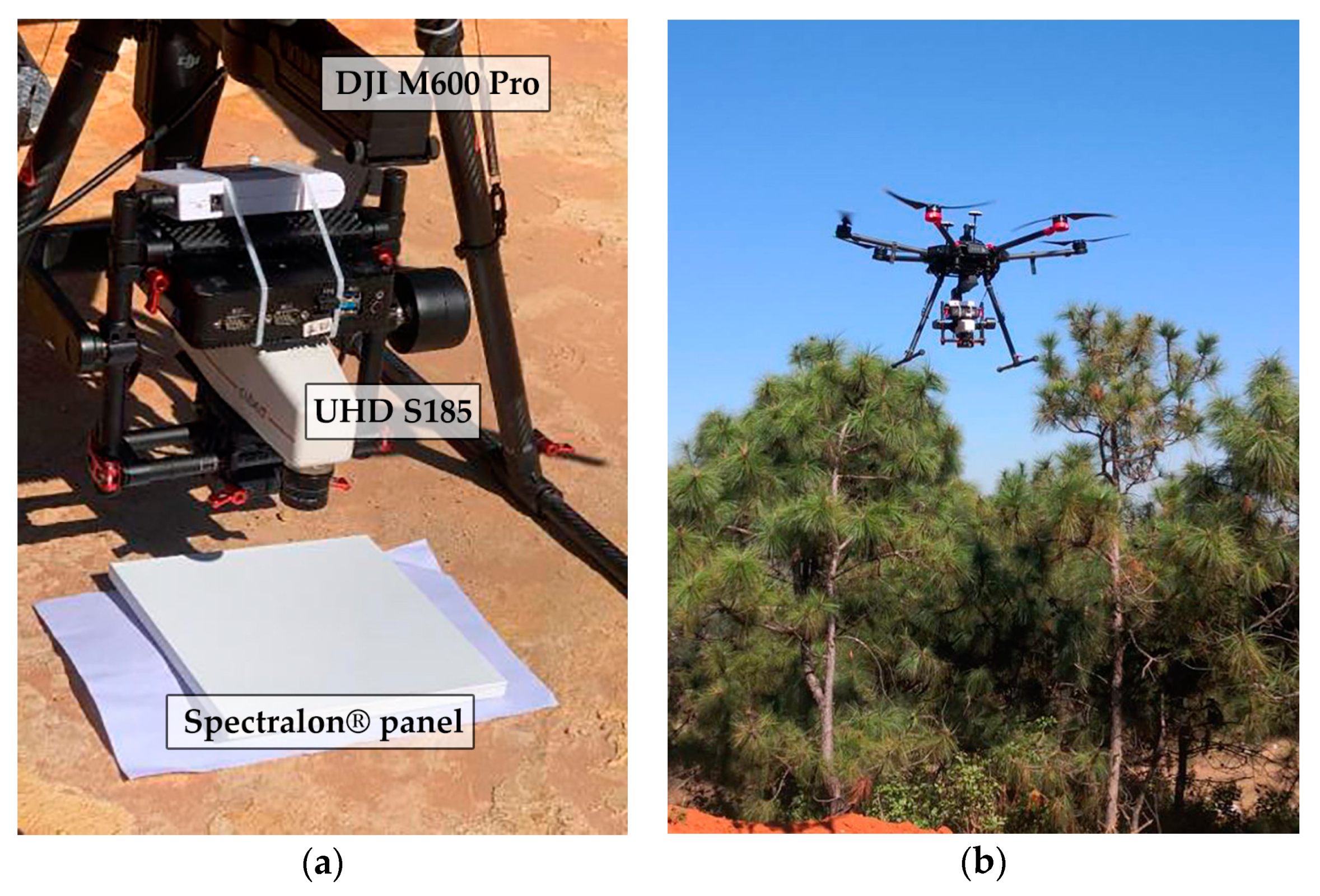
Forests 11 01258 g001
Figure 2. Unmanned aerial vehicle (UAV)-based hyperspectral acquisition equipment. (a) UHD S185, radiometric calibration. (b) The UAV took off and collected data.
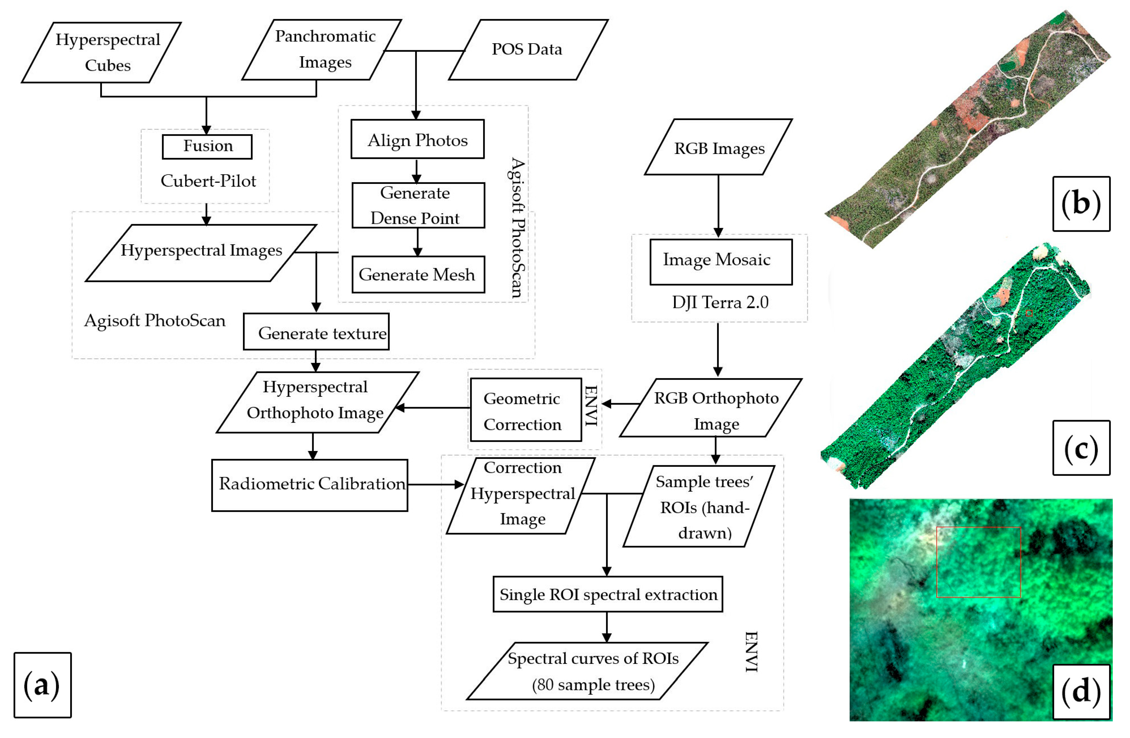
Forests 11 01258 g002
Figure 3. Preprocessing flow. (a) Image preprocessing flow. (b) RGB orthophoto image. (c) Correction hyperspectral image. (d) A local magnification of the hyperspectral image. Position and orientation system (POS); Red-Green-Blue (RGB); Region of interest (ROI).
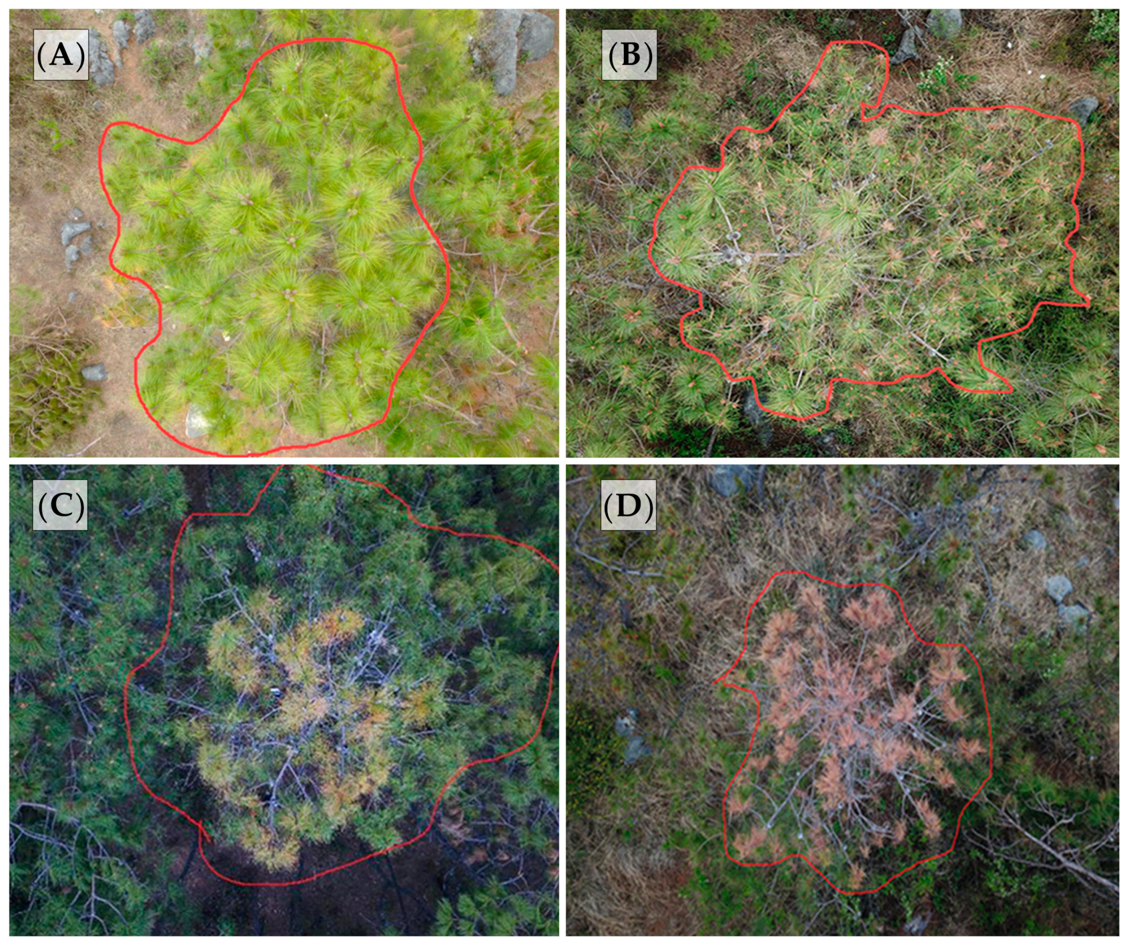
Forests 11 01258 g003
Figure 4. The canopy range of different damage degrees. (A) Healthy. (B) Mild damage. (C) Moderate damage. (D) Severe damage.
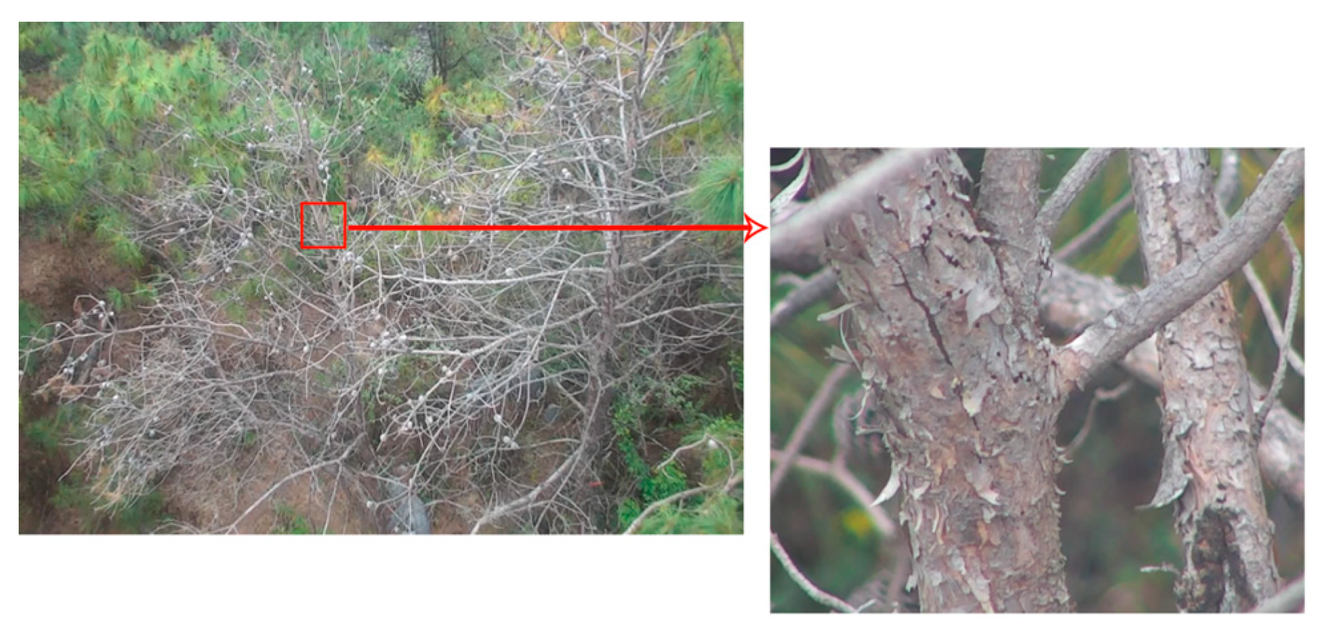
Forests 11 01258 g004
Figure 5. The entrance and exit holes of Pine shoot beetles (PSBs) captured by the M200+Z30.
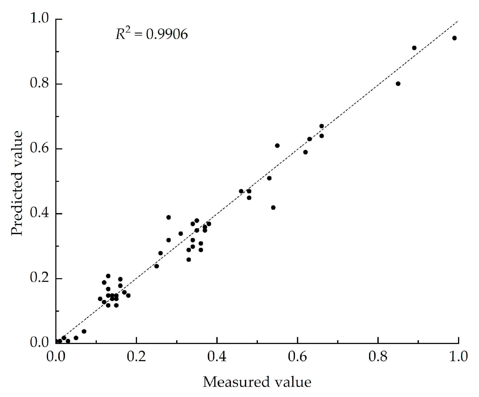
Forests 11 01258 g005
Figure 6. Linear fitting of the measured and predicted values of Ground-DSR.
Forests 11 01258 g006
Figure 7. The curves of Yunnan pine canopies with different degrees of damage. (a) Spectral reflectance curves and (b) first derivative curves.
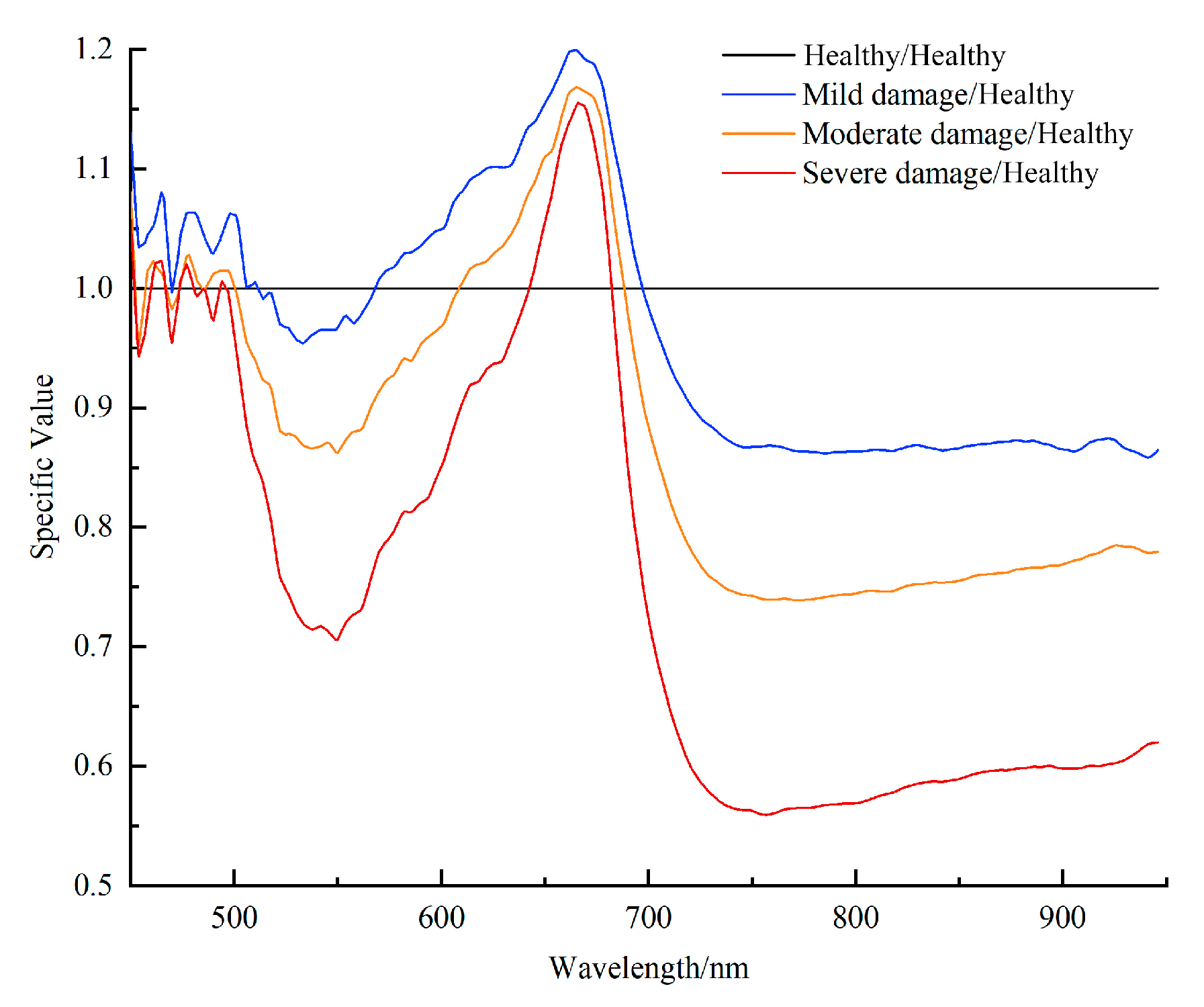
Forests 11 01258 g007
Figure 8. Spectral ratio curves of Yunnan pine canopy.
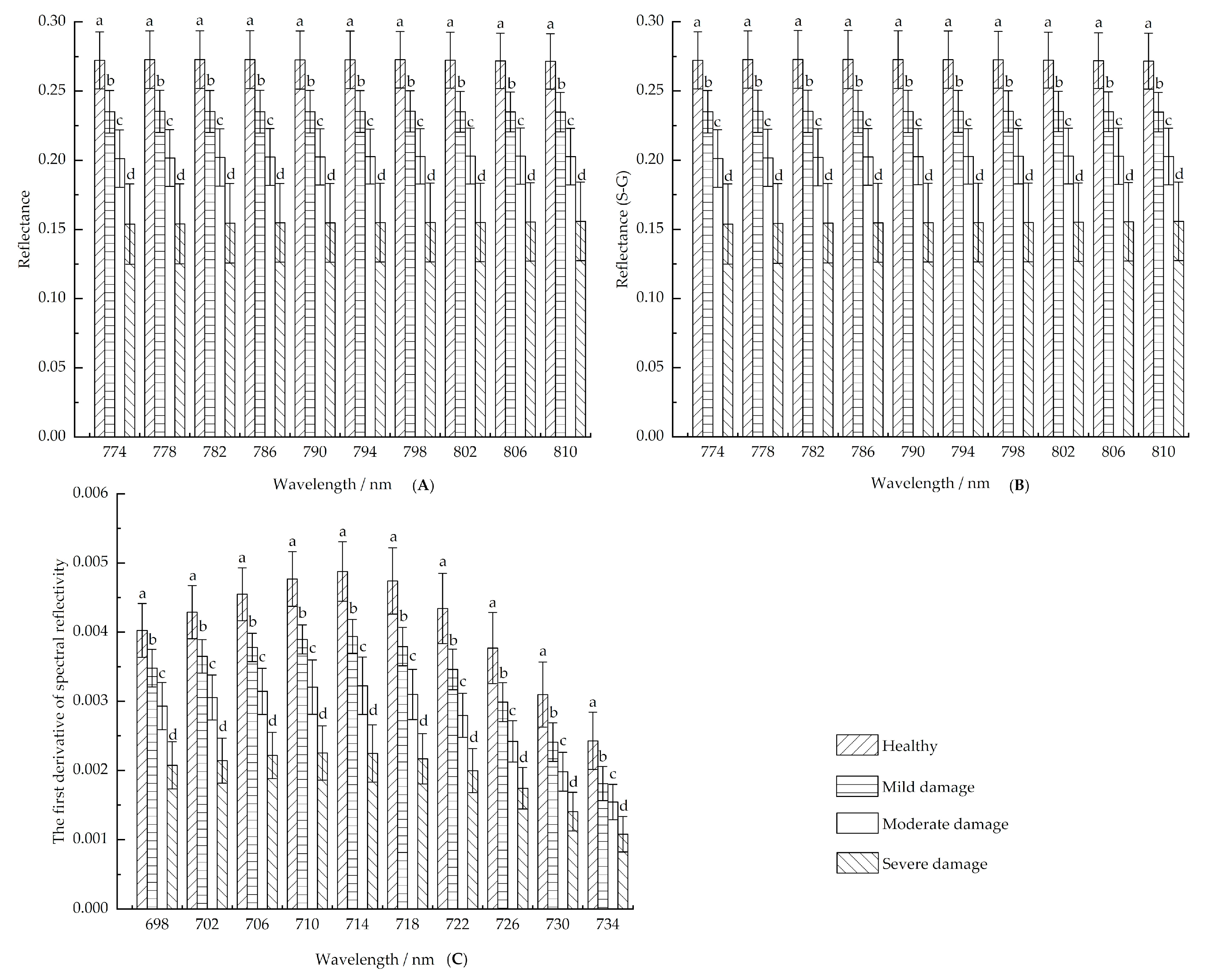
Forests 11 01258 g008
Figure 9. Results of the one-way ANOVA of the wavelengths. (A) The original spectra. (B) The S-G spectra. (C) The first derivative. The data are presented as the mean ± standard error, a, b, c and d indicate that the damage degree is significantly different at this band (p < 0.05), while the same letter indicates that there is no significant difference.
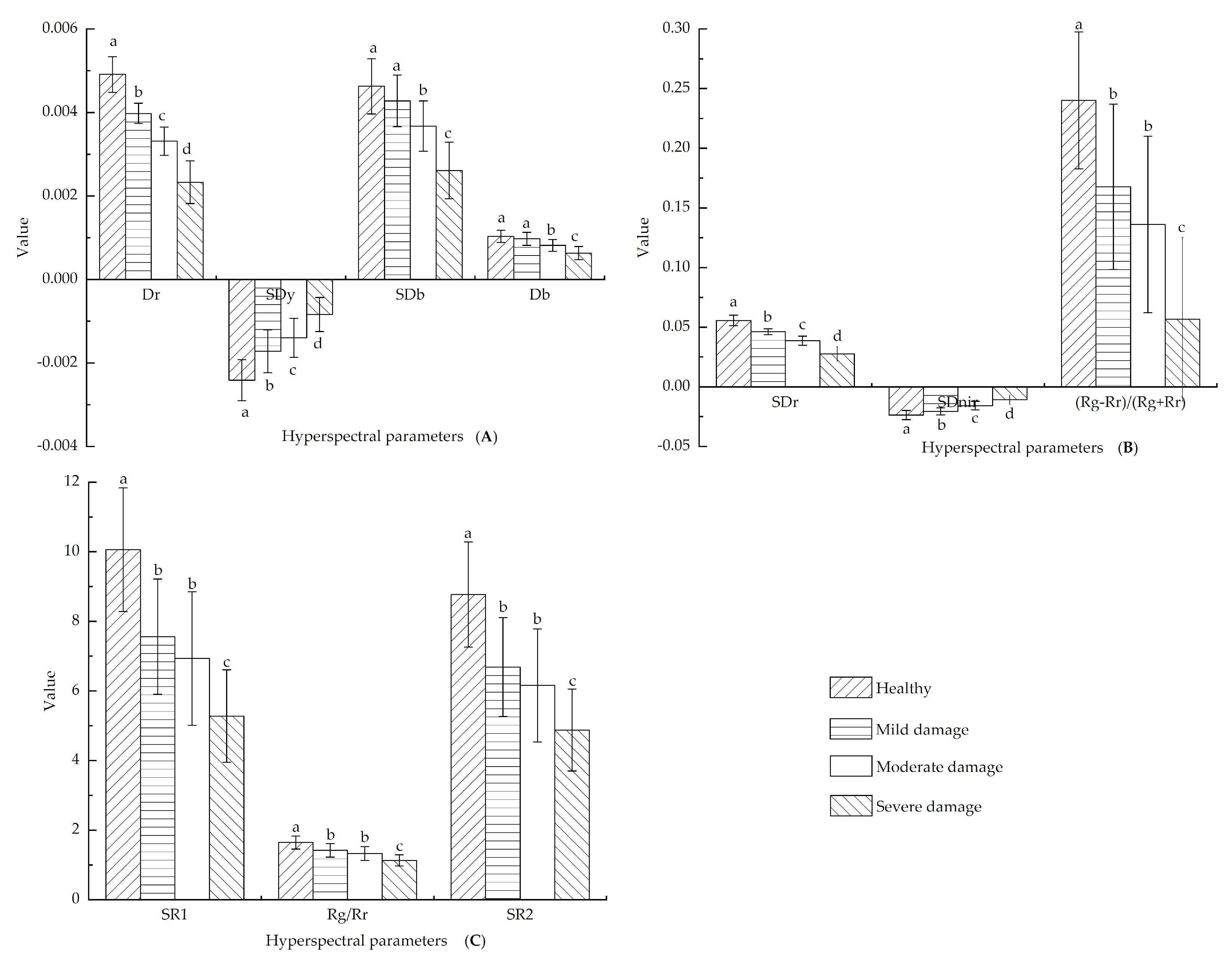
Forests 11 01258 g009
Figure 10. Results of the one-way ANOVA of the hyperspectral parameters. (A) Dr, SDy, SDb, and Db. (B) SDr, SDnir, and (Rg − Rr)/(Rg + Rr). (C) SR1, Rg/Rr, and SR2. a, b, c and d indicate that the damage degree is significantly different at this parameter (p < 0.05), while the same letter indicates that there is no significant difference.
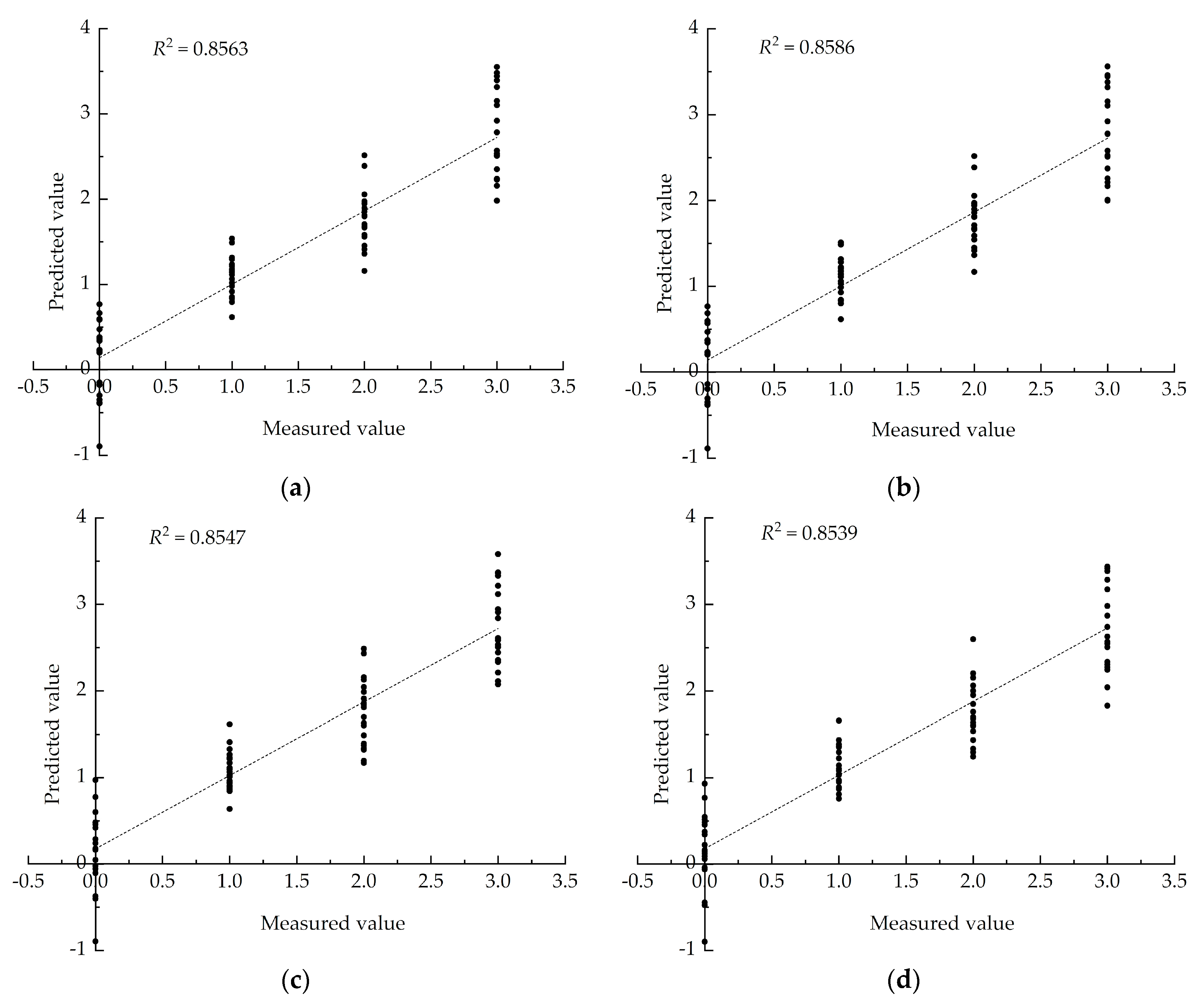
Forests 11 01258 g010
Figure 11. Linear fitting of the measured and predicted values. (a) The original spectral model. (b) The S-G spectral model. (c) The model of the first derivative. (d) The model of hyperspectral parameters.
Forests 11 01258 g011
Table 1. The damage degree of individual Yunnan pine caused by the pine shoot beetle (PSB).
Damage DegreeHealthyMild DamageModerate DamageSevere Damage
Damaged shoot ratio (DSR, %)<1010~2021~50>51
Table 2. Main parameters of the UHD S185 (provided by the manufacturer).
ParametersValueParametersValue
Wavelength range450–950 nmDigital resolution12 bit
Sampling interval4 nmCube resolution1.0 megapixels
Spectral resolution8 nm at 532 nmField of view20°
Spectral channels125Imaging speed5 Cubes/s
Weight470 gSpectral throughput2500 spectra/cube
Table 3. Spectral parameters. Two types of spectral parameters were used in this study: vegetation indices and hyperspectral parameters. We also list specific calculation formulas and describe specific meanings. Normalized Difference Vegetation Index (NDVI); Red Edge Normalized Difference Vegetation Index (NDVI705); Simple Ratio Index (SR); Photochemical Reflectance Index (PRI).
Variable CategoriesVariable Definitions and FormulasReferences
Vegetation indexes NDVI 1 = ( R ¯ ( 760 ~ 850 ) R ¯ ( 650 ~ 670 ) ) ( R ¯ ( 760 ~ 850 ) +   R ¯ ( 650 ~ 670 ) ) [27]
NDVI 2 = ( R 838 R 677 ) / ( R 838 + R 677 ) [28]
NDVI 705 = ( R 750 R 705 ) / ( R 750 + R 705 ) [29]
SR 1 = R ¯ ( 760 ~ 850 ) / R ¯ ( 650 ~ 670 ) [27]
SR 2 = R 838 / R 677 [28]
PRI = ( R 531 R 570 ) / ( R 531 + R 570 ) [27]
Hyperspectral parametersReflectance parametersRg (Green mountain): Maximum reflectance in the wavelength range of 520–560 nm[30]
Rr (Red valley): Minimum reflectance in the wavelength range of 640–680 nm[30]
D = 1 R 670 R 560 + R 760 R 560 760 560 ×   ( 670 560 ) [31]
H = 1 R 500 + R 670 R 500 670 500 ×   ( 560 500 ) R 560 [31]
Rg/Rr[31]
D/H[31]
(Rg − Rr)/(Rg + Rr)[31]
(D − H)/(D + H)[31]
First derivative parametersDb: The maximum value of the first derivative in the blue edge region (470–520 nm)[30]
Dy: The maximum value of the first derivative spectra in the yellow edge region (560–590 nm)[30]
Dr: The maximum value of the first derivative spectra in the red-edge region (660–740 nm)[31]
Dnir: The maximum value of the first derivative spectra in near-infrared region (760–950 nm)[31]
SDb: The sum of the first derivative values in the blue edge region[30]
SDy: The sum of the first derivative values in the yellow edge region[30]
SDr: The sum of the first derivative values in the red-edge region[30]
SDnir: The sum of the first derivative values in the near-infrared region[31]
SDr/SDb[31]
SDr/SDy[31]
SDnir/SDb[31]
SDnir/SDr[31]
(SDr − SDb)/(SDr + SDb)[31]
(SDr − SDy)/(SDr + SDy)[31]
Table 4. Comparison table for Canopy-DSR and Ground-DSR.
Sample NumberDamage DegreeGround-DSRCanopy-DSRLongitudeLatitude
1-001Healthy0.050103.3311424.76616
1-002Healthy0.030103.3324524.76626
2-016Mild damage0.120.19103.3335224.76843
4-013Severe damage0.931103.3376424.77149
Table 5. Fitting equation of Ground-DSR (n = 56) and accuracy validation (n = 24). y is the Ground-DSR obtained by the fitting equation, and x is the Canopy-DSR. Damaged shoot ratio (DSR); Root-mean-square error (RMSE); Relative-root-mean-square error (rRMSE).
Regression Equation of Ground-DSRFitting AccuracyPrediction AccuracyBias
R2RMSErRMSER2RMSErRMSE
y = 0.007 + 1.005x0.9890.0320.0980.9920.0330.072<0.001
Table 6. The results of the correlation analysis and collinearity diagnosis of different spectral processing methods. The Pearson correlation coefficient (PCC) is the result of the Pearson correlation analysis; Tolerance and Variance Inflation Factors (VIF) are the results of the collinearity diagnosis.
The Original SpectraThe S-G SpectraThe First Derivative
BandPCCToleranceVIFBandPCCToleranceVIFBandPCCToleranceVIF
774−0.895 **<0.0013230.847774−0.895 **<0.0012556.225698−0.875 **0.006154.402
778−0.896 **<0.0018201.209778−0.895 **<0.001142,212.548702−0.899 **0.001669.673
782−0.895 **<0.0017197.148782−0.895 **<0.0019926.257706−0.914 **0.001976.484
786−0.895 **<0.0019905.203786−0.895 **<0.001176,513.343710−0.921 **0.0011108.016
790−0.895 **<0.0013117.318790−0.895 **<0.0016018.624714−0.922 **0.001850.018
794−0.896 **<0.00114,842.297794−0.896 **<0.00160,787.606718−0.919 **0.001683.963
798−0.897 **<0.0013659.827798−0.897 **<0.00151,612.218722−0.906 **0.002607.944
802−0.896 **<0.00116,819.991802−0.897 **<0.0014077.492726−0.888 **0.002413.520
806−0.896 **<0.0015105.823806−0.896 **<0.00175,617.265730−0.874 **0.004222.503
810−0.895 **<0.0013302.066810−0.895 **<0.0012483.072734−0.851 **0.02441.300
** represent a significance level of 1%, respectively. r0.05 (n = 80) = 0.217, r0.01 (n = 80) = 0.283.
Table 7. Discriminant analysis results of different spectral processing methods.
MethodBandFisher Discriminant FunctionAccuracy
HealthyMild DamageModerate DamageSevere Damage
The original spectraR798590.800510.114439.481335.99871.30%
(constant)−81.925−61.429−45.953−27.436
The S-G spectraRS-G798589.695509.072439.010335.40871.30%
(constant)−81.735−61.266−45.918−27.380
The first derivativeD71429,055.04723,456.19219,216.08013,381.82980.00%
(constant)−72.215−47.548−32.367−16.411
Table 8. Variable screening results of different spectral processing methods. Screening results were processed through stepwise discriminant analysis. PCCs are the results of the Pearson correlation analysis.
MethodStepVariablePCC
The original spectra1R798−0.897 **
2R690−0.274 *
The S-G spectra1RS-G802−0.897 **
2RS-G690−0.275 **
The first derivative1D714−0.922 **
2D6500.694 **
Hyperspectral parameters1Dr−0.924 **
* and ** represent a significance level of 5% and 1%, respectively. r0.05 (n = 80) = 0.217, r0.01 (n = 80) = 0.283.
Table 9. Stepwise discriminant analysis results for different spectral processing methods. Stepwise discriminant analysis was carried out on the results of four spectral data processing methods and the damage degree. The discriminant coefficient of each degree of damage is listed in Fisher’s discriminant function. Constant represents the constant term in the discriminant function.
MethodBandFisher’s Discriminant FunctionModeling AccuracyCross-Validation
HealthyMild DamageModerate DamageSevere Damage
The original spectraR690−539.930−322.091−227.446−98.19983.80%82.50%
R798788.055627.785522.575371.874
(constant)−93.288−65.472−47.969−27.812
The S-G spectraRS-G690−544.965−327.158−233.401−100.34382.50%78.80%
RS-G802794.239633.431528.802375.697
(constant)−93.823−65.918−48.486−28.076
The first derivativeD650−15,686.086−13,897.181−14,131.4536483.09385.00%85.00%
D71428,460.21622,929.19918,680.20313,627.674
(constant)−72.911−48.095−32.932−16.530
Hyperspectral parametersDr31,819.50025,766.66621,463.58115,099.68186.30%83.80%
(constant)−79.503−52.610−36.930−18.977
Table 10. Multivariate Linear Regression (MLR) model of the damage degree of the Yunnan pine canopy caused by PSB.
ModelRegression EquationFitting AccuracyPrediction AccuracyBias
R2RMSErRMSER2RMSErRMSE
The original spectray = 5.224 + 27.346R690 − 24.592R7980.8640.4160.2770.8220.4720.315−0.068
The S-G spectray = 5.231 + 27.360RS-G690 − 24.623RS-G8020.8620.4190.2790.8270.4650.310−0.067
The first derivativey = 4.855 + 1098.028D650 − 896.053D7140.8610.4200.2800.8210.4740.316−0.051
Hyperspectral parametersy = 5.123 − 1010.441Dr0.8620.4200.2800.8240.4690.313−0.047
Table 11. Quantitative discriminant rules of the damage degree of Yunnan pine canopy caused by PSB (n = 56). The threshold value was determined based on the median of the average values of the two degrees of damage.
ModelValueHealthyMild DamageModerate DamageSevere Damage
The original spectraAverage0.1901.1231.8502.838
Threshold value<0.657(0.657,1.486)(1.486,2.344)≥2.344
The S-G spectraAverage0.1921.1191.8502.838
Threshold value<0.655(0.655,1.484)(1.484,2.344)≥2.344
The first derivativeAverage0.2391.0841.7842.893
Threshold value<0.661(0.661,1.434)(1.434,2.339)≥2.339
Hyperspectral parametersAverage0.2191.1091.8072.867
Threshold value<0.664(0.664,1.458)(1.458,2.337)≥2.337
Table 12. Accuracy test results of the rules (n = 24).
ModelDamage DegreeHealthyMildModerateSevereTest AccuracyOverall Accuracy
The original spectraHealthy6000100.00%87.50%
Mild0600100.00%
Moderate015083.33%
Severe002466.67%
The S-G spectraHealthy6000100.00%83.33%
Mild0600100.00%
Moderate024066.67%
Severe002466.67%
The first derivativeHealthy6000100.00%79.17%
Mild0600100.00%
Moderate024066.67%
Severe003350.00%
Hyperspectral parametersHealthy6000100.0%83.33%
Mild0600100.0%
Moderate015083.33%
Severe003350.00%
Publisher’s Note: MDPI stays neutral with regard to jurisdictional claims in published maps and institutional affiliations.

