Three-Dimensional Evolution of Mesoscale Anticyclones in the Lee of Crete

1. Introduction

Even if the generation of coastal eddies induced by orographic winds have been documented in several studies, it is still difficult to identify what are the main mechanisms that drive their dynamical characteristics (size and intensity) and their vertical extent. The simultaneous combination of several extra processes (coastal currents, bottom friction, tides.) is often a source of complexity for the analysis of real wind-induced eddies. Such eddies could be very intense and/or long-lived, therefore they have a strong impact on the export of coastal nutrients or biogeochemical species into the open sea or the ocean.

The formation of both cyclonic and anticyclonic eddies was frequently observed in the lee of oceanic mountainous islands (Barton et al., 2000; Caldeira, 2002; Jiménez et al., 2008; Piedeleu et al., 2009; Yoshida et al., 2010; Jia et al., 2011; Kersalé et al., 2011; Caldeira and Sangrà, 2012; Couvelard et al., 2012; Caldeira et al., 2014). The Hawaiian archipelago was one of the first case studies that required the use of high-resolution numerical models. The interaction between the North-Equatorial Current and the archipelago is enough to generate eddies, but the use of higher spatial (1/4° degrees instead of 1/2°) and temporal (daily instead of monthly) resolution of wind forcing for the regional models was shown to capture eddy intensities in agreement with the observations (Calil et al., 2008; Jia et al., 2011; Kersalé et al., 2011). For Madeira Island, both numerical simulations (Couvelard et al., 2012) and oceanic observations (Caldeira et al., 2014) indicate that the wind wake induced by the mountain orography could be the dominant mechanism of coastal eddy generation. Larger mountain chains, gaps or valleys could locally amplify the upstream synoptic winds and lead to strong wind-jets on the sea. The numerical study of Pullen et al. (2008) has shown that intensified wind jets in the lee of Mindoro and Luzon Islands induce the generation and the migration of a pair of counter-rotating oceanic eddies. In a similar way, the complex orography of Crete island acts as an obstacle for the wind propagation inducing channeling and deflection of the Etesian winds that impact the regional circulation in the south Aegean Sea and the Levantine basin. This study focuses on this specific area where intense coastal anticyclones are formed recurrently during the summer months (Larnicol et al., 1995; Matteoda and Glenn, 1996; Hamad et al., 2005, 2006; Taupier-Letage, 2008; Amitai et al., 2010; Menna et al., 2012; Mkhinini et al., 2014; Ioannou et al., 2017).

Kotroni et al. (2001) performed simulations with and without Crete and they concluded that the Crete mountain ranges (three mountains in the row with height around 2, 000 m in Figure 1A) modify the Etesian intensity and pathways. The work of Bakun and Agostini (2001) extracts and computes the composite mean wind stress estimates for each one-half degree latitude-longitude quadrangle for the long-term mean seasonal cycle. This observational data-set confirms that the wind-stress curl drives an intense oceanic downwelling at the southeast tip of Crete. Miglietta et al. (2013) simulated the influence of the orography in the same area, capturing the lee waves patterns in the wakes of the Crete, Karpathos, Kasos, and Rhodes islands. The statistical analysis of the monthly surface wind of the ERA-Interim reanalysis (at grid resolution of 1/12°) performed by Mkhinini et al. (2014) exhibits a seasonal correlation between strong negative wind stress curl and the formation of long-lived anticyclones in the eastern Mediterranean Sea. However, correlation does not imply causation and the recent work of Ioannou et al. (2020) provides a dynamical understanding for the formation of long-lived mesoscale anticyclones induced by a seasonal wind-jet that mimics the Etesian winds deflected by Crete island. This study shows that the oceanic response to a symmetric wind jet could be a symmetric dipole or a strongly asymmetric structure dominated by an intense and robust anticyclone. Since, the anticyclonic wind shear, for the mean summer Etesian wind jet, is two times larger than the cyclonic one, the asymmetry of the oceanic response is enhanced and the formation of large mesoscale anticyclones is expected to be favored in this area. Nevertheless, the reduced-gravity rotating shallow-water model used by Ioannou et al. (2020) might be too simple to reproduce the complexity of the oceanic response to the Etesian winds in the southeast of Crete. In order to better understand the different mechanisms involved in the formation of the real wind-induced anticyclones, we performed a high-resolution numerical modeling of the Mediterranean circulation using the CROCO model forced by realistic winds from August 2012 to December 2016. The main advantage of such high-resolution simulation is to describe the rapid dynamics of meso- and sub-mesoscale vortex structures and to have a precise view of their vertical structure. We focus especially on summer and fall 2015 when several Argo floats were present in this area and allowed for a quantitative comparison between the regional model and the in-situ observations. Our main goal is to investigate how the variability of the wind forcing, the complex bathymetry of the shelf or the local outflow impacts on the dynamical characteristics and the vertical extent of these coastal anticyclones.

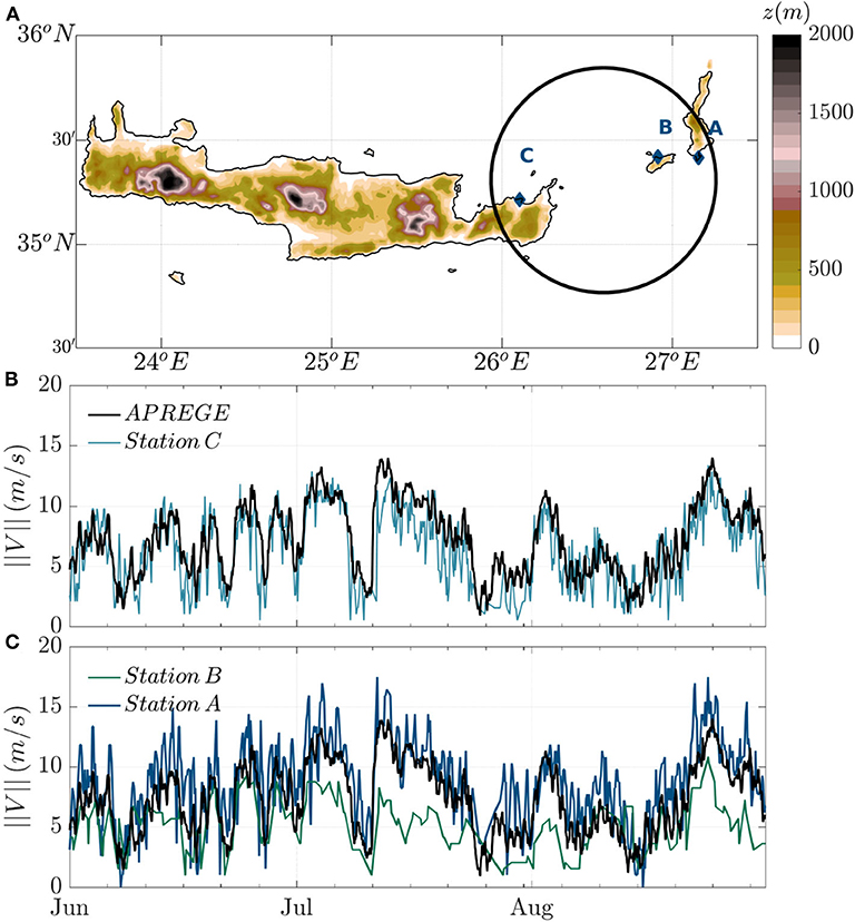
Figure 1. (A) Elevation map (m) of Crete island from ETOPO2 dataset. The locations of the meteorological stations (HNMS); Karpathos (A), Kasos (B), and Sitia (C) are displayed with the blue diamond points. The selected area for analyzing the ARPEGE wind forcing climatology is illustrated with the black circle of R = 60 km. Time-series of wind speed (m/s), as extracted from the three meteorological stations (Station A, B, and C), are shown against the mean wind speed variations from ARPEGE data in (B,C).

The paper is organized as follows. In section 2, we describe the various data-sets used in this study, the ARPEGE winds, the DYNED-Atlas eddy data base and the CROCO ocean model used for our realistic numerical simulations of the Mediterranean Sea in 2015 and 2016. Section 3 presents the dynamical characteristics and the vertical structure of the robust coastal anticyclones which formed at the southeast tip of Crete during summer and fall 2015. Throughout comparisons are carried out between the regional model and remote sensing or in-situ observations. We then discuss, in section 4, the impact of various forcing on the vertical extent of these coastal anticyclones. Finally, we sum up our results and conclude in section 5.

2. Data and Methods

2.1. Regional Wind Forcing

We used the ARPEGE data-set to provide the most realistic wind-forcing for our regional simulations of the Mediterranean Sea. This data-set is based on 4-D variational assimilation of wind observations into the Meteo-France system of Forecast and Analysis ARPEGE. This reanalysis provides the atmospheric fields at high spatial (1/10)° and temporal (hourly 1 h) resolution. To test the accuracy of the ARPEGE data-set in the Crete area and especially in the Kasos strait we collected regional wind speed data from three Meteorological stations of the Hellenic National Meteorological Service (HNMS) located on the islands of Kasos, Karpathos, and Crete at heights 15, 17, and 114 m, respectively. We first build the time series of the mean wind speed in the Kasos strait (inside the black circle of Figure 1A) and compare the temporal variability with the in-situ data of HNMS. We found that the synoptic variability of the ARPEGE data in 2015 and 2016 is in good agreement with the local observations (see Figure 1 for summer 2015). However, if we compare the wind intensities we could find some local discrepancies. There is a correct agreement with the Sitia weather station, which is located at the southeast of Crete, but a slight overestimation is found with the Karpathos station and an underestimation with the Kasos station. Hence, if the main components of the synoptic wind variability in the Kasos area are accurate in the ARPEGE data-set, the local intensities of the surface winds, which are strongly impacted by the complex orography of Crete, should always be taken with care. Nevertheless, as far as we know, this is the best wind data-set available at high resolution for this specific area in 2015 and 2016. The ALADIN data-set used by Mkhinini et al. (2014) has a slightly higher resolution but it ends in 2012.

2.2. CROCO Ocean Model

We use outputs of realistic numerical simulations that were carried out for the Mediterranean Sea using the CROCO numerical model (http://www.croco-ocean.org). We refer to Shchepetkin and McWilliams (2005) and Debreu et al. (2012) as well as to Auclair et al. (2018) for details regarding the CROCO inherited numerics from ROMS, its barotropic time-stepping set-up and its solver. The simulation under investigation, CROCO-MED60v40-2015, was forced at the ocean top with ARPEGE wind forcing, thanks to the classical bulk COARE formula (Fairall et al., 2003) that takes into account the wind stress acting on the ocean surface as

where ${\rho }_{air}=1.25kg{m}^{-3}$ is the air density, C_d the drag coefficient that varies based on the exchanges between the atmosphere-ocean turbulent surface heat fluxes and U the surface wind. The simulation domain covers the total Mediterranean Sea, extending from 7°W to 36.23°E and from 30.23°S to 45.82°N. The model configuration solves the classical primitive equations in an horizontal resolution of 1/60° in both longitudinal and latitudinal directions, a well fitted resolution to capture the dynamics of interest. The vertical coordinate used is a generalized terrain following one. It is a stretched coordinate that allows to keep flat levels near the surface whatever the bathymetry gradient. The stretching coordinate parameters at the surface (θ_s) and at the bottom (θ_b), are set to θ_s = 6 and θ_b = 0, respectively. Forty unevenly distributed vertical levels discretized the water column. They are closer one from each other next to the surface and more spaced by the bottom where the vertical gradients of hydrology parameters (temperature or salinity) are weak. This distribution was designed in order to properly catch the intense surface dynamics. Moreover, the bathymetry has been produced at SHOM for modeling purposes (http://www.10.12770/50b46a9f-0c4c-4168-9d1c-da33cf7ee188, http://www.data.datacite.org/10.6096/MISTRALS.1341) and was built up from DTM at 100 and 500 m resolution that was optimally interpolated at first and then smoothed to control the pressure gradient truncation error associated with the terrain following coordinate system (Shchepetkin and McWilliams, 2003). The bottom viscous stress has a quadratic form of variable drag coefficient (C_d) computed with the log law approximation. The initial and boundary conditions were built from CMEMS global system analysis (GLOBAL OCEAN 1/12° PHYSICS ANALYSIS AND FORECAST UPDATED DAILY), optimally interpolated on the computational grid. CROCO-MED60v40-2015 is a result of a free run simulation (no nudging nor assimilation of any kind) that started on the 1st of August 2012 when the water column stability is at its maximum to avoid static instability in the spinning up phase of three years. It ran till the end of December 2016. For the purposes of this paper, we extracted oceanic numerical fields for the year 2015. To track and quantify full trajectories of mesoscale eddies reproduced in the model, we used AMEDA eddy detection algorithm (Le Vu et al., 2018). Adapted to CROCO 1/60° numerical fields, AMEDA can identify the eddy characteristics from the daily mean surface geostrophic velocities derived from Sea Surface Height of the model averaged during 24 h.

2.3. Eddy Database DYNEDAtlas

In order to compare the mesoscale eddies formed in the southeast of Crete in the regional simulation CROCO-MED60v40-2015 with both remote sensing and in-situ observations, we used the dynamical eddy data-base DYNED-Atlas (https://www.lmd.polytechnique.fr/dyned/). This recent data-base provides 17 years (2000–2017) of eddy detection and tracking in the Mediterranean Sea along with the co-localization of Argo floats for each detected eddy (https://doi.org/10.14768/2019130201.2). The dynamical characteristics of the eddies contained in the DYNED-Atlas database were computed by the AMEDA eddy detection algorithm (Le Vu et al., 2018) applied on daily surface velocity fields. The latter were derived from the Absolute Dynamic Topography (ADT) maps produced by Salto/Duacs and distributed by CMEMS with a spatial resolution of 1/8° which is much coarser than the spatial resolution of the numerical simulations. Hence, we will compare in this study only the characteristics of mesoscale eddies having a characteristic radius R_max (i.e., the radius where the azimuthal velocity V_max is maximal) higher than 15 km. In order to estimate the vertical structures of the detected eddies, DYNED-Atlas uses all the Argo profiles available since 2000 in the Mediterranean Sea. Once all the detected eddies are identified during the 2000–2017 period, we can separate the Argo profiles in two groups: the ones that are located inside an eddy (i.e., inside the last closed streamline) and the ones which are outside of all the detected eddies. With the second group we can build unperturbed climatological profiles (T, S and ρ) around a given position and a given date. We consider here all the Argo profiles (out of eddies) located at <150 km around the selected position and at ±30 days from the target day during the 17 years. Such climatological profiles (plotted in black) give a reference for the T, S and ρ profiles associated to an unperturbed ocean (i.e., without coherent eddies). Hence, the difference between this climatological density profile with the Argo profile taken inside an eddy allows us to compute the profile of the density anomaly ${\sigma }_A(z)(kg{m}^{-3})$ and estimate its vertical extent as shown in Figure 2. We use the depth of the maximal density anomaly Z_max to quantify the vertical extent of the eddy. A similar methodology was used to estimate the depth of the coastal anticyclones in the regional simulation CROCO-MED60v40-2015 and perform quantitative comparisons with the DYNED-Atlas data. Since all the physical fields are available in the numerical model, the core eddy density profile corresponds to an average of all profiles located at <10 km from the eddy center. The background profile corresponds to an average of all the vertical profiles located along the last closed streamline.

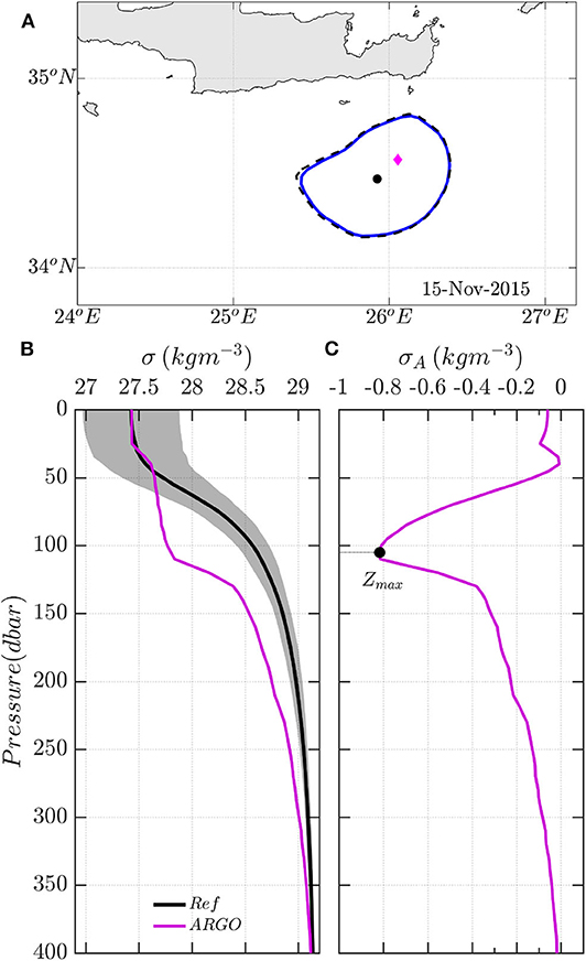
Figure 2. (A) Position of the O_IE15 in November 2015. The eddy characteristic and last contour are illustrated with the blue solid and black dashed lines. The position of an Argo float trapped inside the eddy is shown with the magenta diamond. Vertical (B) density σ and (C) density anomaly σ_A profile of the Argo float trapped inside the O_IE15 (magenta color). The black line shows the mean climatological profile as computed by Argo profiles that are detected outside of eddies.

3. Results

3.1. Etesian Wind-Forcing and Formation of Coastal Anticyclones

The Etesian winds blowing across the complex orography of Crete induce strong wind jets in its wake. As shown by Ioannou et al. (2020) such orographic winds could lead to the formation of long-lived mesoscale anticyclones in this area. We show in Figure 3 the seasonal variations of both the surface wind stress and the wind stress curl of the ARPEGE wind reanalysis for the year 2015. We note that the intensity of the negative wind stress curl in the Kasos strait (area inside the circle of Figure 3) is not strictly correlated to the wind intensity (Figures 3E,F). For this specific year, the maximum wind intensity occurs in February while intense negative wind stress curls occur in July. During the summer months, strong wind jets occur with a large area of negative Ekman pumping (deep blue area in Figure 3C) that extents a hundred of kilometers away from the Kasos strait and tends to favor the formation of coastal anticyclones. It can therefore be expected that the long-lived Ierapetra anticyclone (IE15) will form in July or early August this year. However, this was not the case. Indeed, a long-lived anticyclone that survives more than 6 months was formed in late September in the numerical simulation CROCO-MED60v40-2015 while a similar eddy was detected in early October in the DYNED-Atlas database. Such long-lived and robust anticyclone, which is formed in the Southeast of Crete, is usually called an Ierapetra anticyclone and will be labeled M_IE15 in what follows. Nevertheless, according to CROCO-MED60v40-2015, several other anticyclones were formed in the same area during summer 2015. These coastal anticyclones (labeled AE1, AE2, and AE3) were formed the 9 of June, the 14 of August, and the 12 of September, respectively (Figure 4). The lifetime of these robust eddies does not exceed 3 months. This is still low compared to the M_IE15, which survives more than 15 months. Hence, the realistic simulation CROCO-MED60v40-2015 reveals that several coastal anticyclones are formed in the Kasos strait area when intense wind-jets, driven by the Etesian winds, occur. Among all these robust coastal anticyclones, only one will survive more than 6 months and will have the dynamical characteristics of an Ierapetra eddy.

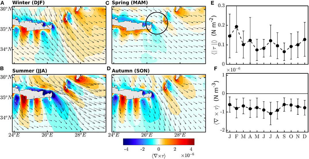
Figure 3. Climatological wind stress 〈τ〉 (vectors) and wind stress curl 〈∇ × τ〉 (colors) during 2015 for the winter (A), spring (B), summer (C), and autumn (D) months based on ARPEGE wind data. The selected area for analyzing the wind forcing climatology is illustrated with the black circle in (B). The mean monthly climatological variations of wind stress 〈τ〉 and wind stress curl 〈∇ × τ〉 are shown in (E,F), respectively.

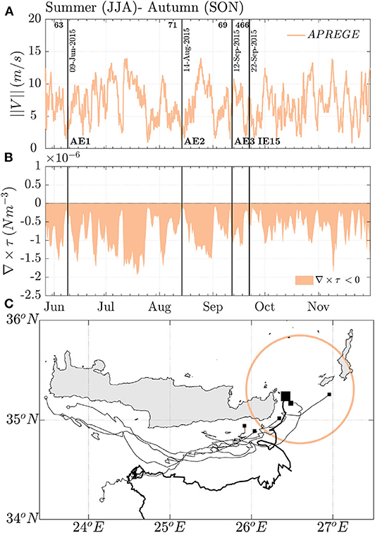
Figure 4. Time-series of (A) wind speed (m/s) and (B) negative wind stress curl 〈∇ × τ〉 are shown with the orange color as extracted from ARPEGE wind data. The selected area for analyzing the wind forcing climatology is illustrated with the orange circle in (C). Trajectories of long-lived (> 2 weeks) eddies (gray colors) detected in CROCO model in the southeastern lee of Crete island during the summer and autumn of 2015. The first points of the eddy detection are plotted with the black square points while the points of last detection are illustrated with the open white circles. The longest-lived detected anticyclone is illustrated with the thick black line.

3.2. Comparison Between the CROCO Model and the DYNED-Atlas Data-Base

A regional model that runs without assimilation, such as the CROCO-MED60v40-2015 is very unlikely to reproduce the exact dynamics and trajectory of mesoscale eddies. However, if the wind forcing is correct in the Kasos strait (as shown in the Figure 1), the wind-induced coastal anticyclones should have similar characteristics both in the model and the observations. Therefore, a systematic comparison is made between the dynamical eddy characteristics of the CROCO-MED60v40-2015 numerical model and the observations compiled in the Mediterranean eddy data-base: DYNED-Atlas. Besides, such analysis will help to quantify the dynamical differences between the numerous coastal anticyclones which are formed during summer months and the long-lived Ierapetra Eddy (IE15).

3.2.1. Dynamical Characteristics and Trajectories

The Figure 5 compares the temporal evolution of the characteristic radius (R_max) and the intensity (V_max) of the long-lived M_IE15 formed in CROCO-MED60v40-2015 with the O_IE15 detected in DYNED-Atlas. These two mesoscale anticyclones were formed mid-fall at the end of September or early October, respectively. Since the spatial resolution of the numerical model (1/60°) is seven times greater than that of merged altimetry products (1/8°), it makes sense that the initial formation of such coastal eddy is better detected in the regional simulation CROCO-MED60v40-2015. If we assume that the model simulates correctly the IE formation, the AMEDA algorithm will detect it earlier in the regional model than in the coarse AVISO/CMEMS data set. In both cases, the radius of the M_IE15 and the O_IE15 exceeds the local deformation radius (R_d = 10 − 12 km) by at least a factor three (Figure 5B). Such large radius is in good agreement with previous observations of Ierapetra Eddies (Matteoda and Glenn, 1996; Hamad et al., 2006; Taupier-Letage, 2008; Mkhinini et al., 2014; Ioannou et al., 2017, 2019).

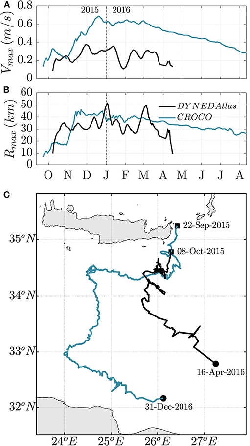
Figure 5. (A) Temporal evolution of long-lived Ierapetra anticyclones as detected in 2015 with AMEDA algorithm from DYNED-Atlas eddy database and from CROCO-MED60v40-2015 simulation. The dynamical characteristics of the eddy velocity V_max (m/s) and eddy radius R_max (km) are shown in (A,B), respectively while their trajectories are illustrated in (C).

However, the eddy intensity seems to reach higher values in the numerical model than in the eddy database. The maximal azimuthal velocity V_max could reach up to 70 cm/s in the CROCO-MED60v40-2015 while it never exceeds 40 cm/s in the DYNED-Atlas data base (Figure 5A). The underestimation of the IE's intensity in AVISO/CMEMS products, in comparison with in-situ measurements, was previously documented in Ioannou et al. (2017) and typical velocity values of 60 cm/s were confirmed by VMADCP measurements for IE eddies (Ioannou et al., 2017, 2019). The trajectory of the simulated (M_IE15) and the observed one (O_IE15) also differs, even if both of them quickly propagate offshore 60 km south of the Kasos strait (Figure 5C).

As in the numerical model, a shorter-lived coastal anticyclone, that remained close to the shore in the southeast of Crete, was also detected the 29 of July according to the DYNED Atlas data-base. Such coastal anticyclone was detected from altimetry despite its decreased accuracy near the coast. The formation and the location of the short-lived anticyclone was also confirmed by a careful analysis of SST images. Hence, both remote sensing data sets, visible images, and altimetry maps, show that coastal anticyclones could be formed in this area earlier during the summer months. We compare in the Figure 6, the dynamical characteristics of this coastal anticyclone detected in the DYNED-Atlas with the three structures formed by the regional simulation in June, August, and early September. These anticyclones are smaller and weaker than the IE15, their characteristic radius R_max does not exceed 25 km while the maximal azimuthal velocities V_max remain in the range of 20−40 cm/s. More strikingly, they all seem to follow the same type of trajectory. The centers of these eddies remain attached to the coastline of Crete and the anticyclone stays above shelf even if they propagate westward, far away from their formation area (Figure 6C). Hence, the dynamical characteristics of these wind-induced eddies differ significantly from the long-lived Ierapetra anticyclone.

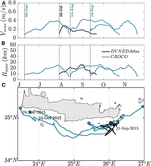
Figure 6. (A) Temporal evolution of short-lived coastal anticyclones detected in 2015 with AMEDA algorithm from DYNED-Atlas eddy database and from CROCO-MED60v40-2015 simulation. The dynamical characteristics of the eddy, its velocity V_max (m/s) and radius R_max (km) are shown in (A,B), respectively while their trajectories are illustrated in (C). The evolution and the trajectory of the anticyclones AE1, AE2, and AE3 tracked in the regional model are plotted with blue lines while the observed anticyclone (DYNED-Atlas data-base) is plotted with a black line.

3.2.2. Comparison of Vertical Eddy Characteristics

The growing number of Argo floats deployed in the Mediterranean Sea in recent years makes it possible to characterize more precisely the three-dimensional evolution of long-lived eddies. Fortunately, the Ierapetra Eddy was sampled by several Argo profiles in the autumn of 2015 just after its formation and later on during winter 2016. The Figure 7 shows the temporal evolution of the density anomaly in the core of the Ierapetra anticyclone according to the Argo profiles taken in November 2015, in January 2016, and in February 2016. We select here only the profiles that were located at a distance of <35 km from the eddy center (Figure 7A). The maximal density anomaly induced by the eddy on the climatological density background that contains no eddy signature was then estimated. As expected for an anticyclonic eddy, the density anomaly is negative. Moreover, we compute the depth of the maximal density anomaly Z_max (black dots in Figures 7B–D) to quantify the vertical extent of the O_IE15.

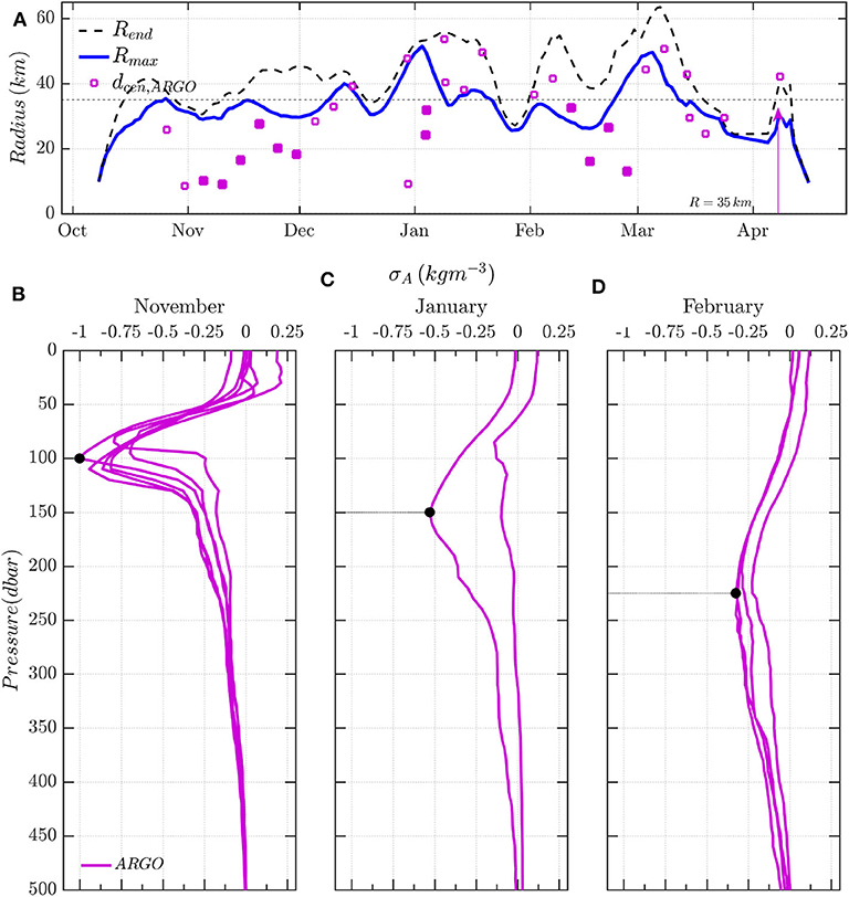
Figure 7. (A) Temporal evolution of the O_IE15 eddy characteristic contour (blue line) and the last contour (black dashed line) as extracted from the DYNED-Atlas eddy database. The squared points illustrate the position of the Argo profiles as a function of their distance from the eddy center. Vertical profiles of density anomaly ${\sigma }_A(kg{m}^{-3})$ are shown for the months of (B) November 2015, (C) January 2016, and (D) February 2016 as obtained from the Argo float profiles that were trapped in the O_IE15.

According to Figure 7B, one month after its first detection, the density anomaly is confined between 50 and 125 m, with a maximum anomaly of ${\sigma }_A=-1kg{m}^{-3}$ located at −100 m. Few months later, in January and in February 2016, the maximal density anomaly propagated in depth, down to Z_max = −150 m and Z_max = −225 m, respectively, but decreased in amplitude. The significant deepening of the O_IE15, during the winter months, coincides with the seasonal deepening of the mixed layer depth in the Mediterranean Sea (Moschos et al., 2020). During winter months, when the air-sea interactions are strong, the mixed layer could reach deeper values in the anticyclonic eddy core in comparison with the surroundings (Kouketsu et al., 2011; Dufois et al., 2016). We found that the mixed layer could go down to 200 m inside the Ierapetra eddy in February 2016. It is then very simple to quantify the vertical extent of the M_IE15 that is formed in the CROCO-MED60v40-2015 and compare them with the in-situ observations. Since we can track the eddy center with a high accuracy in the model, we can easily follow the temporal evolution of the density anomaly within the eddy core. The Figure 8 presents the monthly average of this anomaly for M_IE15 in comparison with the Argo profiles in November 2015, January 2016, and February 2016. The model is in correct agreement with the in-situ observations (Figures 8B–D) and exhibits the same trend: a significant deepening of the M_IE15 during winter months. However, the maximal density anomaly reaches deeper values, down to Z_max = −220 m and Z_max = −240 m in January and February 2016, in CROCO-MED60v40-2015. The main advantage of such a realistic regional model is that it is possible to follow the three-dimensional evolution of all eddies and to compare them with each other. We could then check how the vertical structure of the coastal anticyclones, that are formed during summer months, differs from the long-lived Ierapetra anticyclone. The Figure 9 shows the temporal evolution of the size, the intensity, and the vertical core density anomaly of one short-lived coastal anticyclone (AE3) in comparison with the M_IE15. We observe that during the initial stage of formation (the month that follows the first detection) these two types of anticyclones exhibit the same vertical structure and a moderate value of the radius R_max around 20 km. It is about a month later (in November 2015) that the Ierapetra anticyclone changes its structure: it increases in size and intensity as it expands in depth. Hence, it appears that the deepening of this long-lived anticyclone is induced by a dynamical process which is independent from its initial generation. The initial structure and the dynamical characteristics of the Ierapetra eddy, few weeks after its formation, does not differ significantly from the coastal anticyclones that are generated in summer by the wind-jet channelized by the Kasos strait. It is later on, during the winter months, that another mechanism leads to a drastic change in the vertical and the horizontal extent of the M_IE15.

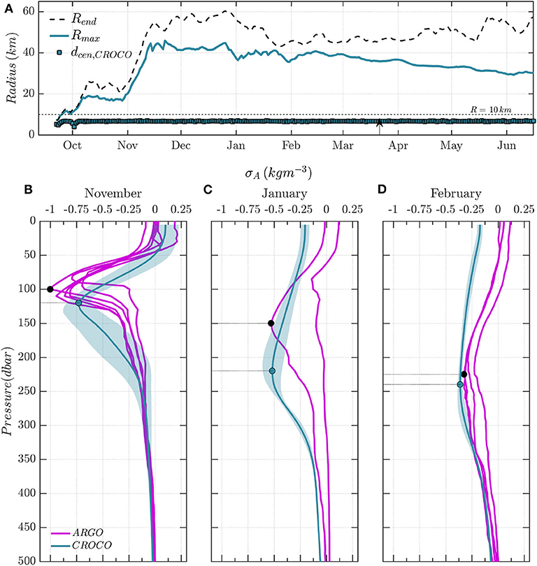
Figure 8. (A) Temporal evolution of the M_IE15 eddy characteristic contour (solid line) and the last contour (black dashed line) computed with AMEDA algorithm applied on CROCO geostrophic fields. Vertical profiles of density anomaly ${\sigma }_A(kg{m}^{-3})$ for the months of (B) November 2015, (C) January 2016, and (D) February 2016 as obtained from the Argo float profiles that were trapped in the O_IE15 (shown with magenta color) and as obtained from the M_IE15 in CROCO-MED60v40-2015 simulation for the same period (shown with the blue color).

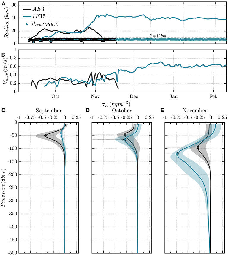
Figure 9. Temporal evolution of dynamical characteristics of (A) velocity V_max (m/s) and (B) radius R_max (km) for the coastal eddies AE3 and M_IE15 as computed with AMEDA algorithm applied on CROCO geostrophic fields. Comparison between the vertical profiles of density anomaly ${\sigma }_A(kg{m}^{-3})$ are shown for the months of (C) September 2015, (D) October 2015, and (E) November 2015 for the two anticyclones AE3 and M_IE15 from the CROCO-MED60v40-2015 simulation.

4. Discussion

Several coastal anticyclones were formed during summer and fall 2015 at the southeast tip of Crete, but only one of them will evolve into a large, deep, and long-lived Ierapetra Eddy. Distinct physical processes could lead to this dynamical evolution. On one hand, the orographic wind-jets that occur in the wake of Crete induce strong and localized Ekman pumping. These upwelling or downwelling could then re-intensify or attenuate some coastal eddies. The intensification of a pre-existing mesoscale anticyclone was confirmed by in-situ observations (Ioannou et al., 2017) and idealized numerical simulations (Ioannou et al., 2020). If all these coastal anticyclones seem to be wind driven, their lifetime does not seem to be correlated with the wind-jet intensity in the Kasos strait and probably some more complex mechanisms should be considered to explain the robustness and the lifetime of the M_IE15. On the other hand, the Aegean outflow through the Kasos strait (Kontoyiannis et al., 1999, 2005) may also contribute to the formation of coastal eddies or interact with them in this area and therefore modify their intensity and their vertical extent. Both processes are discussed in what follows.

4.1. Wind-Eddy Interactions

We first investigate the impact of local winds on coastal anticyclones once they are formed. We track these eddies with the AMEDA algorithm and compute for each of them the evolution of the daily averaged surface wind-stress inside the eddy contour. The local wind-stress curl will drive horizontal divergence and convergence of the Ekman transport and induce a mean vertical Ekman pumping inside the eddy (Ekman, 1905; Stern, 1965). The cumulative effect of this local Ekman pumping could lead to a significant isopycnal displacement. In order to take into account the core vorticity of the coastal anticyclones we use the non-linear relation derived by Stern (1965). Assuming a quasi-steady response (i.e., neglecting inertial waves generation) the additional isopycnal displacement Δη induced by the cumulative wind-forcing is given by the following relation:

where t = t₀ is the beginning of the eddy detection, ρ the density of water, f the Coriolis parameter, ζ the vorticity within the eddy core and A the area enclosed by a radial distance of 1.5 R_max of the maximum eddy contour. The surface wind stress τ is estimated by the bulk formula:

where the drag coefficient C_d is set constant $C_d=1.610^{-3}$ and V_wind is the 10 m wind speed. We plot in Figure 10A the temporal evolution of the cumulative isopycnal displacement induced in the core of the three coastal anticyclones (AE1, AE2, and AE3) in comparison with the Ierapetra anticyclone M_IE15. For all the anticyclones, the vortex intensity V_max follows the temporal evolution of the cumulative Ekman pumping (Figures 10A,B). Indeed, the azimuthal velocity V_max of AE1, AE3, and M_IE15 reached their highest values, respectively in July, November and December 2015 when the wind-induced isopycnal displacement reaches its maximum value for each eddy. For AE2, the wind-stress curl, in the eddy core, is zero or negative and therefore, unlike the other ones, the intensity of AE2 stays roughly constant in August and starts to decay in September. However, if the short-lived anticyclones AE1 and AE3 experienced a similar Ekman pumping than the long-lived M_IE15, their intensity and their vertical extents differ strongly from Ierapetra 2015. Thus, for the same wind-stress curl amplitude, the dynamic response can be very different from one anticyclone to another. It seems that the intensity and vertical extent of the Ierapetra anticyclone is more strongly intensified by the local wind forcing than of the other eddies.

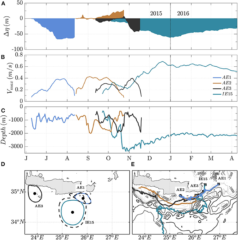
Figure 10. Comparison between the temporal evolution of the anticyclones AE1, AE2, AE3, and M_IE15. The isopycnal displacements after generation Δη(m), associated with the wind stress curl 〈∇ × τ〉 extracted above the eddies (in an area of 30 km from the eddy center) are illustrated in (A). The temporal evolution of the eddy characteristic velocities V_max and the mean depth along the eddy trajectories are shown in (B,C) for the different anticyclones. The eddy contours and trajectories of the different anticyclones are shown in (D) and (E). The background map shown in (E) corresponds to the CROCO model bathymetry.

One of the main differences between the M_IE15 and the other coastal anticyclones lies in their trajectories. Quite rapidly, after its formation, the Ierapetra eddy escapes from the shore and propagates into deep water unlike other eddies that travel along the Crete coast. The seabed under the eddies AE1, AE2, and AE3 is between −600 and −1, 000 m, when the wind forcing is strong, while, in November–December 2015, when Ierapetra anticyclone intensifies, the seabed stays below −2, 000 m and may reaches −3, 000 m depth (Figures 10C,E). Hence, the bottom friction could be a possible explanation of the limitation of the intensity and the isopycnal downwelling of these short-lived coastal eddies. Moreover, according to the Figure 10D, the characteristic eddy contours of AE1 and AE3 tangent the Crete coastline in July and November 2015 when the cumulative Ekman pumping is maximum for these eddies. The alongshore dissipation could also attenuate the wind induced intensification of these coastal eddies.

The temporal evolution of the vertical density structure and the cumulative isopycnal displacement η = Z_max(t₀) + Δη, induced by the local Ekman pumping, are shown in Figure 11 for AE1, AE2, AE3, and M_IE15, respectively. We find that the depth of maximal density anomaly Z_max follows roughly the evolution of η. Even if the numerical values are not strictly equal, these two characteristic depths are very close in the first months of the eddy lifetime. This correct agreement between the temporal evolution of Δη (given by the Equation 2) and Z_max confirms that the local wind-stress curl drives the vertical structure of these anticyclones few months after their formation. However, we note for the Ierapetra eddy that during winter months (December, January, and February) the density anomaly deepens while the isopycnal downwelling, induced by the wind-stress curl (i.e., Δη), does not increase. We also notice, during this period, that the intensity of the maximal density anomaly weakens from ${\sigma }_A=-1kg{m}^{-3}$ mid-November to ${\sigma }_A=-0.3kg{m}^{-3}$ mid-February. Such an evolution is probably due to air-sea fluxes at the surface that tend to extract a significant amount of heat from the mixed layer that deepens into the anticyclonic core (Donners et al., 2004). Such heat fluxes are not taken into account in the Equation (2). Hence, in addition to the local wind-shear, the air-sea fluxes could have a significant impact, especially during winter months, on the vertical structure of long-lived mesoscale anticyclones.

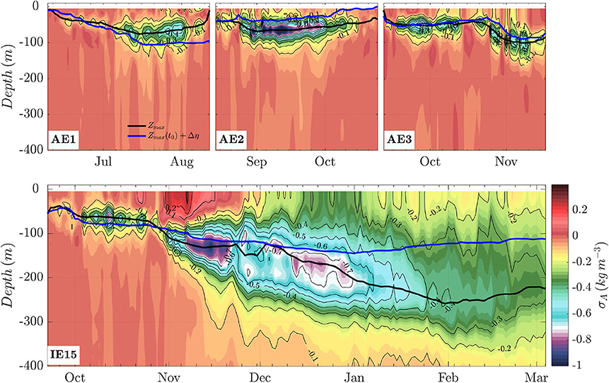
Figure 11. Comparison between the vertical profiles of density anomaly ${\sigma }_A(kg{m}^{-3})$ for the AE1, AE2, AE3, and M_IE15 anticyclones generated during summer and fall period in the CROCO-MED60v40-2015 simulation southeast of Crete. The temporal evolution of the minimum density anomaly Z_max and the isopycnal displacement Δη associated with the wind stress curl above the eddies are illustrated with the black and blue lines, respectively.

4.2. Kasos Strait Outflow

Another forcing mechanism that could generate strong anticyclonic eddies is the density bulge induced by river or strait outflows. A well-know example, at the entrance of the Mediterranean Sea, is the intense Alboran gyre which is forced by the fresh Atlantic water which enters through the Gibraltar strait. Such anticyclone is mainly driven by the amplitude of the inflow rather than the local wind forcing (Viúdez et al., 1996a,b; Viúdez, 1997; Gomis et al., 2001; Flexas et al., 2006).

It is therefore questionable whether the flow out of the Kasos Strait can control the formation of the long-lived Ierapetra anticyclones. Some snapshots of the surface circulation show that the jet corresponding to the Kasos strait outflow, seems to be connected with the periphery of the Ierapetra anticyclone (Figure 12A). Therefore, we first quantify the Kasos strait outflow and its variability in CROCO-MED60v40-2015 (Figures 12B,C) both in the surface (0−200 m) and the subsurface layers (below −200 m). This outflow of lighter water coming from the Aegean Sea could be quite significant with a total flow rate that could exceed 2.4 Sv during few days, in July, August, or November 2015. We then compare the variability of this outflow with the intensity of the coastal anticyclones (AE1, AE2, AE3) and the M_IE15 that stays in the vicinity of the Kasos strait (i.e., the area delimited by the black box in Figure 12A). We find that the intensification of the AE1 in July and the M_IE15 in November seems to be both correlated to the outflow intensity according to the Figures 12C,D. We should note that the eddy intensification is always associated to an amplification of the density anomaly (Figure 12E). However, the outflow is relatively strong during the whole period and we can also observe the intensification of AE3 without a significant change in the outflow of the Kasos strait. Hence, there is no systematic correlation between the variations of the outflow and the intensification (of V_max or σ_A) of pre-existing anticyclones in this area.

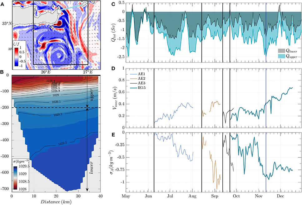
Figure 12. (A) Surface vorticity fields ζ/f and (B) vertical section of the density σ(kg/m⁻³) in the Kasos Strait for the 11 November 2015. Temporal evolution of the Kasos Strait outflow Q separated in surface (0 − 200 m) and subsurface outflow (200 − 700 m) in (C). The dates shown with the vertical black lines indicate the first detection of long-lived anticyclones during the same period. The temporal evolution of the eddy characteristic velocity V_max and the density anomaly σ_A is shown for the different anticyclones AE1, AE2, AE3, and M_IE15 in (D,E).

5. Summary and Conclusions

Using a high-resolution (1/60°) regional model CROCO-MED60v40, we analyzed the formation of a coastal eddy in the southeastern wake of Crete island. It is in this area that an intense, large-scale and long-lived anticyclone is formed almost every year, commonly known as the Ierapetra eddy (Hamad et al., 2005, 2006; Taupier-Letage, 2008; Amitai et al., 2010; Menna et al., 2012; Mkhinini et al., 2014; Ioannou et al., 2017). Our previous studies (Mkhinini et al., 2014; Ioannou et al., 2020) have confirmed that the intensity of the summer wind jets (i.e., Etesian winds) blowing through the Kasos strait is one of the main reasons for the formation of robust anticyclones in this area. Motivated by the fact that the regional model CROCO-MED60v40 was driven by the ARPEGE hourly wind reanalysis (at 1/10°), which are the most accurate wind dataset in this region, we study the relation between the wind forcing and the dynamical characteristics of the wind-induced eddies. More specifically, we focus on the year 2015 where an Ierapetra eddy was formed both in the observational as well as in the numerical fields. During that year, Argo profilers were trapped for several months (October 2015–April 2016) in the core of the Ierapetra anticyclone, allowing us to compare the evolution of the vertical structure of the anticyclone from the in-situ data with the numerical outputs.

Even without in-situ data assimilation, the numerical model was able to reproduce the formation and the dynamical evolution of a long-lived and robust anticyclone (M_IE15) similar to the Ierapetra eddy (O_IE15) that was detected this specific year. The M_IE15 was formed at the end of September while the O_IE15 was detected in early November according to the DYNED-Atlas eddy data-base. The temporal evolution of the characteristic radius and the vertical extent of the M_IE15 are also very close to the observations. However, the trajectories of these two eddies diverge after a few weeks and the eddy intensity reach higher values in the numerical model than in the eddy database. The latter could be due to a systematic under-evaluation of the eddy amplitude when we use the sea surface height or the surface velocity field derived from the altimetry data-set. Indeed, similar under-evaluation in comparison with local VMADCP measurements were found by Ioannou et al. (2017, 2019).

More surprisingly, according to CROCO-MED60v40-2015, several other anticyclones were formed in the same area during summer 2015 when the Etesian winds reach strong values. Three of them survive more than 2 months but their trajectories differ from the M_IE15. These coastal anticyclones travel along the Crete shelf while the Ierapetra eddy propagates offshore after its formation. A careful analysis of the DYNED-Atlas eddy data base reveals that a similar coastal anticyclone was also detected, during August and September 2015, on the standard AVISO/CMEMS Mediterranean altimetry data. Hence, such coastal anticyclones that propagate along the south coast of Crete are both present in the model and the observations. Thus, even if it does not exactly reproduce the observed ocean circulation (since there is no data assimilation), the regional simulation CROCO-MED60v40-2015 seems to provide a realistic description of the formation and the evolution of coastal eddies in the south of Crete island. Therefore, we can rely on this high-resolution model to study the impact of the orographic wind forcing on the formation and the subsequent evolution of realistic coastal anticyclones.

We do find that the intensity of the wind-induced Ekman pumping acting on the eddies, once they are formed, modulates their intensity. However, these coastal anticyclones respond differently to the wind forcing if they remain close to the coast, in shallow-waters, or if they propagate offshore in deep water. The impact of the bottom friction or the coastal dissipation seems to limit the wind amplification of coastal eddies. Among all the coastal anticyclones, which are formed by the summer intensification of the wind jet, only the one that escapes from the shelf will lead to a deep and long-lived eddy. Hence, a strong surface wind-jet is not enough to form an Ierapetra anticyclone and several others factors play a role. The wind-induced Ekman pumping should occur when the eddy is in deep waters and presumably the outflow from the Kasos strait reinforces this mechanism. Moreover, during winter, strong air-sea fluxes could result in a significant upper-layer oceanic heat loss, that could enhance the vertical mixing within the eddy core and deepen its mixed layer. However, these assumptions must be confirmed by a longer numerical simulation that will allow to investigate the formation of different Ierapetra anticyclones several years in a row.

Data Availability Statement

The raw data supporting the conclusions of this article will be made available by the authors, without undue reservation.

Author Contributions

AI and AS designed the study, performed the data analysis, and contributed to the writing. FD performed the numerical simulation CROCO-MED60v40 and provided guidance in the interpretation of the results of the numerical simulation. BL adapted the AMEDA algorithm to perform the automatic eddy detection on the numerical simulations. All authors contributed to the article and approved the submitted version.

Conflict of Interest

The authors declare that the research was conducted in the absence of any commercial or financial relationships that could be construed as a potential conflict of interest.

Acknowledgments

This work and especially AI and BL were funded by the SHOM with research contract Catoobs 18CP01. The Hellenic National Meteorological Service (HNMS) is kindly acknowledged for providing the wind observations used in this study.

References

Amitai, Y., Lehahn, Y., Lazar, A., and Heifetz, E. (2010). Surface circulation of the eastern Mediterranean Levantine basin: insights from analyzing 14 years of satellite altimetry data. J. Geophys. Res. 115:C10058. doi: 10.1029/2010JC006147
Auclair, F., Bordois, L., Dossmann, Y., Duhaut, T., Paci, A., Ulses, C., et al. (2018). A non-hydrostatic non-Boussinesq algorithm for free-surface ocean modelling. Ocean Model. 132, 12–29. doi: 10.1016/j.ocemod.2018.07.011
Bakun, A., and Agostini, V. N. (2001). Seasonal patterns of wind-induced upwelling/downwelling in the Mediterranean Sea. Sci. Mar. 65, 243–257. doi: 10.3989/scimar.2001.65n3243
Barton, E. D., Basterretxea, G., Flament, P., Mitchelson-Jacob, E. G., Jones, B., Arístegui, J., et al. (2000). Lee region of Gran Canaria. J. Geophys. Res. 105, 17173–17193. doi: 10.1029/2000JC900010
Caldeira, R., and Sangrá, P. (2012). Complex geophysical wake flows Madeira Archipelago case study. J. Ocean Dyn. 62, 683–700. doi: 10.1007/s10236-012-0528-6
Caldeira, R. M. A., and Marchesiello, P. (2002). Ocean response to wind sheltering in the Southern California Bight. Geophys. Res. Lett. 29, 1–4. doi: 10.1029/2001GL014563
Caldeira, R. M. A., Stegner, A., Couvelard, X., Araújo, I. B., Testor, P., and Lorenzo, A. (2014). Evolution of an oceanic anticyclone in the lee of Madeira Island: in situ and remote sensing survey. J. Geophys. Res. 119, 1195–1216. doi: 10.1002/2013JC009493
Calil, P. H., Richards, K. J., Jia, Y., and Bidigare, R. R. (2008). Eddy activity in the lee of the Hawaiian Islands. Deep Sea Res. II 55, 1179–1194. doi: 10.1016/j.dsr2.2008.01.008
Couvelard, X., Caldeira, R., Araújo, I., and Tomé, R. (2012). Wind mediated vorticity-generation and eddy-confinement, leeward of the Madeira Island: 2008 numerical case study. Dyn. Atmos. Oceans 58, 128–149. doi: 10.1016/j.dynatmoce.2012.09.005
Debreu, L., Marchesiello, P., Penven, P., and Cambon, G. (2012). Two-way nesting in split-explicit ocean models: algorithms, implementation and validation. Ocean Model. 49–50, 1–21. doi: 10.1016/j.ocemod.2012.03.003
Donners, J., Drijfhout, S., and Coward, A. (2004). Impact of cooling on the water mass exchange of Agulhas rings in a high resolution ocean model. Geophys. Res. Lett. 31:L16312. doi: 10.1029/2004GL020644
Dufois, F., Hardman-Mountford, N. J., Greenwood, J., Richardson, A. J., Feng, M., and Matear, R. J. (2016). Anticyclonic eddies are more productive than cyclonic eddies in subtropical gyres because of winter mixing. Sci. Adv. 2:e1600282. doi: 10.1126/sciadv.1600282
Ekman, W. (1905). On the influence of the Earth's Rotation on Ocean-Currents. Arkiv Fur Matematik Astronomi Och Fysik 11, 355–367.
Fairall, C. W., Bradley, E. F., Hare, J. E., Grachev, A. A., and Edson, J. B. (2003). Bulk parameterization of air-sea fluxes: updates and verification for the COARE algorithm. J. Clim. 16, 571–591. doi: 10.1175/1520-0442(2003)016<0571:BPOASF>2.0.CO;2
Flexas, M., Gomis, D., Ruiz, S., Pascual, A., and León, P. (2006). In situ and satellite observations of the eastward migration of the Western Alboran Sea Gyre. Prog. Oceanogr. 70, 486–509. doi: 10.1016/j.pocean.2006.03.017
Gomis, D., Ruiz, S., and Pedder, M. (2001). Diagnostic analysis of the 3D ageostrophic circulation from a multivariate spatial interpolation of CTD and ADCP data. Deep Sea Res. I 48, 269–295. doi: 10.1016/S0967-0637(00)00060-1
Hamad, N., Millot, C., and Taupier-Letage, I. (2005). A new hypothesis about the surface circulation in the eastern basin of the Mediterranean sea. Prog. Oceanogr. 66, 287–298. doi: 10.1016/j.pocean.2005.04.002
Hamad, N., Millot, C., and Taupier-Letage, I. (2006). The surface circulation in the eastern basin of the Mediterranean Sea. Sci. Mar. 70, 457–503. doi: 10.3989/scimar.2006.70n3457
Ioannou, A., Stegner, A., Dubos, T., Le Vu, B., and Speich, S. (2020). Generation and intensification of mesoscale anticyclones by orographic wind jets: the case of Ierapetra eddies forced by the etesians. J. Geophys. Res. 125:e2019JC015810. doi: 10.1029/2019JC015810
Ioannou, A., Stegner, A., Le Vu, B., Taupier-Letage, I., and Speich, S. (2017). Dynamical evolution of intense ierapetra eddies on a 22 year long period. J. Geophys. Res. 122, 9276–9298. doi: 10.1002/2017JC013158
Ioannou, A., Stegner, A., Tuel, A., Le Vu, B., Dumas, F., and Speich, S. (2019). Cyclostrophic corrections of AVISO/DUACS surface velocities and its application to mesoscale eddies in the Mediterranean Sea. J. Geophys. Res. 124, 8913–8932. doi: 10.1029/2019JC015031
Jia, Y., Calil, P. H. R., Chassignet, E. P., Metzger, E. J., Potemra, J. T., Richards, K. J., et al. (2011). Generation of mesoscale eddies in the lee of the Hawaiian Islands. J. Geophys. Res. 116:C11009. doi: 10.1029/2011JC007305
Jiménez, B., Sangrá, P., and Mason, E. (2008). A numerical study of the relative importance of wind and topographic forcing on oceanic eddy shedding by tall, deep water islands. Ocean Model. 22, 146–157. doi: 10.1016/j.ocemod.2008.02.004
Kersalé, M., Doglioli, A. M., and Petrenko, A. A. (2011). Sensitivity study of the generation of mesoscale eddies in a numerical model of Hawaii islands. Ocean Sci. 7, 277–291. doi: 10.5194/os-7-277-2011
Kontoyiannis, H., Balopoulos, E., Gotsis-Skretas, O., Pavlidou, A., Assimakopoulou, G., and Papageorgiou, E. (2005). The hydrology and biochemistry of the Cretan Straits (Antikithira and Kassos Straits) revisited in the period June 1997–May 1998. J. Mar. Syst. 53, 37–57. doi: 10.1016/j.jmarsys.2004.06.007
Kontoyiannis, H., Theocharis, A., Balopoulos, E., Kioroglou, S., Papadopoulos, V., Collins, M., et al. (1999). Water fluxes through the Cretan Arc Straits, Eastern Mediterranean Sea: March 1994 to June 1995. Prog. Oceanogr. 44, 511–529. doi: 10.1016/S0079-6611(99)00044-0
Kotroni, V., Lagouvardos, K., and Lalas, D. (2001). The effect of the island of Crete on the Etesian winds over the Aegean Sea. Q. J. R. Meteorol. Soc. 127, 1917–1937. doi: 10.1002/qj.49712757604
Kouketsu, S., Tomita, H., Oka, E., Hosoda, S., Kobayashi, T., and Sato, K. (2011). The role of meso-scale eddies in mixed layer deepening and mode water formation in the western North Pacific. J. Oceanogr. 68, 63–77. doi: 10.1007/s10872-011-0049-9
Larnicol, G., Traon, P.-Y. L., Ayoub, N., and Mey, P. D. (1995). Mean sea level and surface circulation variability of the Mediterranean Sea from 2 years of TOPEX/POSEIDON altimetry. J. Geophys. Res. 100:25163. doi: 10.1029/95JC01961
Le Vu, B., Stegner, A., and Arsouze, T. (2018). Angular momentum eddy detection and tracking algorithm (AMEDA) and its application to coastal eddy formation. J. Atmos. Ocean. Technol. 35, 739–762. doi: 10.1175/JTECH-D-17-0010.1
Matteoda, A. M., and Glenn, S. M. (1996). Observations of recurrent mesoscale eddies in the eastern Mediterranean. J. Geophys. Res. 101, 20687–20709. doi: 10.1029/96JC01111
Menna, M., Poulain, P.-M., Zodiatis, G., and Gertman, I. (2012). On the surface circulation of the Levantine sub-basin derived from Lagrangian drifters and satellite altimetry data. Deep Sea Res. Part I 65, 46–58. doi: 10.1016/j.dsr.2012.02.008
Miglietta, M. M., Zecchetto, S., and Biasio, F. D. (2013). A comparison of WRF model simulations with SAR wind data in two case studies of orographic lee waves over the Eastern Mediterranean Sea. Atmos. Res. 120–121, 127–146. doi: 10.1016/j.atmosres.2012.08.009
Mkhinini, N., Coimbra, A. L. S., Stegner, A., Arsouze, T., Taupier-Letage, I., and Béranger, K. (2014). Long-lived mesoscale eddies in the eastern Mediterranean Sea: analysis of 20 years of AVISO geostrophic velocities. J. Geophys. Res. 119, 8603–8626. doi: 10.1002/2014JC010176
Moschos, E., Stegner, A., Schwander, O., and Gallinari, P. (2020). Classification of eddy sea surface temperature signatures under cloud coverage. IEEE J. Select. Top. Appl. Earth Observ. Rem. Sens. 13, 3437–3447. doi: 10.1109/JSTARS.2020.3001830
Piedeleu, M., Sangrá, P., Sánchez-Vidal, A., Fabrés, J., Gordo, C., and Calafat, A. (2009). An observational study of oceanic eddy generation mechanisms by tall deep-water islands (Gran Canaria). Geophys. Res. Lett. 36, 1–5. doi: 10.1029/2008GL037010
Pullen, J., Doyle, J. D., May, P., Chavanne, C., Flament, P., and Arnone, R. A. (2008). Monsoon surges trigger oceanic eddy formation and propagation in the lee of the Philippine Islands. Geophys. Res. Lett. 35:L07604. doi: 10.1029/2007GL033109
Shchepetkin, A. F., and McWilliams, J. C. (2003). A method for computing horizontal pressure-gradient force in an oceanic model with a nonaligned vertical coordinate. J. Geophys. Res. 108:3090. doi: 10.1029/2001JC001047
Shchepetkin, A. F., and McWilliams, J. C. (2005). The regional oceanic modeling system (ROMS): a split-explicit, free-surface, topography-following-coordinate oceanic model. Ocean Model. 9, 347–404. doi: 10.1016/j.ocemod.2004.08.002
Stern, M. E. (1965). Interaction of a uniform wind stress with a geostrophic vortex. Deep Sea Res. Oceanogr. Abstracts 12, 355–367. doi: 10.1016/0011-7471(65)90007-0
Taupier-Letage, I. (2008). “On the use of thermal images for circulation studies: applications to the eastern Mediterranean basin,” in Remote Sensing of the European Seas, eds V. Barale and M. Gade (La Seyne/Mer: Springer Netherlands), 153–164. doi: 10.1007/978-1-4020-6772-3_12
Viúdez, Á. (1997). An explanation for the curvature of the Atlantic jet past the strait of Gibraltar. J. Phys. Oceanogr. 27, 1804–1810. doi: 10.1175/1520-0485(1997)027<1804:AEFTCO>2.0.CO;2
Viúdez, Á., Haney, R. L., and Tintoré, J. (1996a). Circulation in the Alboran Sea as determined by quasi-synoptic hydrographic observations. Part II: mesoscale ageostrophic motion diagnosed through density dynamical assimilation. J. Phys. Oceanogr. 26, 706–724. doi: 10.1175/1520-0485(1996)026<0706:CITASA>2.0.CO;2
Viúdez, Á., Tintoré, J., and Haney, R. L. (1996b). Circulation in the Alboran Sea as determined by quasi-synoptic hydrographic observations. Part I: three-dimensional structure of the two anticyclonic gyres. J. Phys. Oceanogr. 26, 684–705. doi: 10.1175/1520-0485(1996)026<0684:CITASA>2.0.CO;2
Keywords: wind-forced anticyclones, orographic wind forcing, Ierapetra eddies, Ekman pumping, Island wakes, coastal eddies
Citation: Ioannou A, Stegner A, Dumas F and Le Vu B (2020) Three-Dimensional Evolution of Mesoscale Anticyclones in the Lee of Crete. Front. Mar. Sci. 7:609156. doi: 10.3389/fmars.2020.609156
Received: 22 October 2020; Accepted: 03 November 2020;
Published: 25 November 2020.
Edited by:
Miguel A. C. Teixeira, University of Reading, United KingdomReviewed by:
Jesus Dubert, University of Aveiro, PortugalIvica Vilibic, Institute of Oceanography and Fisheries, Croatia
Copyright © 2020 Ioannou, Stegner, Dumas and Le Vu. This is an open-access article distributed under the terms of the Creative Commons Attribution License (CC BY). The use, distribution or reproduction in other forums is permitted, provided the original author(s) and the copyright owner(s) are credited and that the original publication in this journal is cited, in accordance with accepted academic practice. No use, distribution or reproduction is permitted which does not comply with these terms.
*Correspondence: Artemis Ioannou, innartemis@gmail.com