Evaluating the Performance of a Max-Stable Process for Estimating Intensity-Duration-Frequency Curves


1
Institute of Meteorology, Freie Universität Berlin, Carl-Heinrich-Becker-Weg 6-10, 12165 Berlin, Germany
2
Wupperverband, Untere Lichtenplatzer Str. 100, 42289 Wuppertal, Germany
*
Author to whom correspondence should be addressed.
Water 2020, 12(12), 3314; https://doi.org/10.3390/w12123314
Submission received: 27 September 2020
/
Revised: 21 November 2020
/
Accepted: 23 November 2020
/
Published: 25 November 2020
(This article belongs to the Special Issue Extreme Value Analysis of Short-Duration Rainfall and Intensity–Duration–Frequency Models)
Abstract
:To explicitly account for asymptotic dependence between rainfall intensity maxima of different accumulation duration, a recent development for estimating Intensity-Duration-Frequency (IDF) curves involves the use of a max-stable process. In our study, we aimed to estimate the impact on the performance of the return levels resulting from an IDF model that accounts for such asymptotical dependence. To investigate this impact, we compared the performance of the return level estimates of two IDF models using the quantile skill index (QSI). One IDF model is based on a max-stable process assuming asymptotic dependence; the other is a simplified (or reduced) duration-dependent GEV model assuming asymptotic independence. The resulting QSI shows that the overall performance of the two models is very similar, with the max-stable model slightly outperforming the other model for short durations (). From a simulation study, we conclude that max-stable processes are worth considering for IDF curve estimation when focusing on short durations if the model’s asymptotic dependence can be assumed to be properly captured.
1. Introduction
Much research has been recently done on the application of multivariate methods to estimate Intensity-Duration-Frequency (IDF) curves. IDF curves are a popular tool among hydrologists to estimate exceedance probabilities of extreme rainfall events with different durations. In broad terms, IDF curves model a relationship between intensities of extreme rainfall events and their frequencies (i.e., return periods) as a function of event duration. A challenge in estimating IDF curves is how to deal with the simultaneous modeling of intensities for different durations, in particular, how to account for the possible dependence that could arise between intensities of different durations.
Initially, the conventional approach to model IDF curves was based on univariate extreme value theory (EVT) models. Early work on the topic estimates extreme value distributions individually for several fixed durations and subsequently fits an empirical relation to quantiles (return levels) as a function of duration [1,2,3,4]. This approach is prone to inconsistencies as the natural ordering of quantiles is not guaranteed to be preserved over all durations (in other words: quantiles cross). To address this problem, Koutsoyiannis et al. [5] suggested a consistent extreme value model for intensities as a function of duration with location and scale being functions of duration. Later on, a couple of studies implemented methods from Bayesian statistics for the univariate relationship between intensity and duration. Lehmann et al. [6] formulated a Bayesian Hierarchical Model (BHM) based on the model from [5], and Van de Vyver [7] presented a multi-scale model using Bayesian inference. More recently, Ritschel et al. [8] used this model to characterize stochastic precipitation models, and Ulrich et al. [9] proposed the addition of spatial covariates to the model from Koutsoyiannis et al. [5], extending the work of Fischer et al. [10] using spatial covariates to model daily precipitation maxima. These studies make an assumption of stationarity, which may not be valid under a changing climate. Some recent studies have focused on tackling this issue with univariate methods to construct consistent IDF curves in a nonstationary setting. Some examples include the work of Padulano et al. [11] using the storm index method, as well as those of Ganguli and Coulibaly [12], Ganguli and Coulibaly [13] comparing the estimates from a stationary and nonstationary method.
Many of the previous univariate models assume that rainfall intensities are independent for different durations, thus simplifying the modeling efforts. However, the estimation of an extreme value distribution as a function of durations brings along the problem of dependence of extremes associated with different durations, as longer duration series are always aggregated from series of shorter durations. An important consequence of this way of aggregating is that there exists no “single” event for any given duration. As an example, the values of the 15 min duration events are not events that lasted exactly 15 min, but rather the “largest” 15 min long average values from longer events.
In recent years there has been widespread use of multivariate EVT methods for modeling IDF curves, which allow the explicit modeling of dependence structures that could not be captured by the univariate approach. Essentially, a multivariate extreme value distribution (MEVD) is fitted to extreme precipitation data, with the marginal distributions being frequently modeled by a univariate extreme value distribution. Simultaneously, the dependence structure is described with methods such as max-stable processes or copulas. An early example of this was proposed by Muller et al. [14] who, alongside the independence likelihood (analogous to the univariate approach), proposed the use of a so-called trivariate likelihood for three durations: 1, 24, and 72 h. In this study, the dependence between 24 and 72 h was modeled with a bivariate extreme distribution from the logistic family. Afterward, Van de Vyver [15] investigated the use of the trivariate likelihood by calculating the parameters’ uncertainty using a Bayesian approach. He found that, while the resulting posterior distributions from the trivariate likelihood were narrower than the independence likelihood ones, its limitations were too strict to recommend its use over the independence likelihood. An early example of modeling IDF curves using copulas is the study of Singh and Zhang [16], who used a Frank Archimedean copula to estimate the IDF relationship in a bivariate setting.
Some of the most recent advances have been a result of studies that attempted to model IDF curves within a spatial setting. These approaches take advantage of the methods developed for modeling so-called spatial extremes [17]. For example, Stephenson et al. [18] implemented a spatial max-stable process for IDF estimation; they estimated IDF curves in a spatial setting by incorporating a Bayesian Hierarchical Model in every station with a max-stable process. While their approach was able to capture the spatial dependence, they had to limit their scope to assume that the rainfall maxima were independent for different durations. Later on, Tyralis and Langousis [19] proposed the use of a max-stable process to estimate IDF curves for a single station in a way that the asymptotic dependence between rainfall intensity maxima of different durations was explicitly modeled, extending the spatial methodology by proposing a so-called duration space instead of geographical coordinates. Remarkably, their proposed max-stable process was able to explicitly account for the asymptotic dependence between intensities for different durations.
Although Tyralis and Langousis [19] demonstrated the feasibility of a duration-dependent max-stable process to estimate IDF curves, they did not investigate their performance compared to, e.g., univariate EVT methods. Their results showed that both the univariate and multivariate approaches adequately approximated the empirical quantiles, where the max-stable approach resulted in more conservative (i.e., higher) intensities for large quantiles (i.e., longer return periods). In our study, we aimed to build upon the results of Tyralis and Langousis [19] by estimating the impact on performance when accounting for the asymptotical dependence between rainfall intensity aggregated over different durations. We expected that, whenever the asymptotical dependence between durations is high and the max-stable approach is able to capture the “strength” of such dependence for the estimated intensities, the model performance should be significantly higher than for a model assuming independence.
The present paper introduces a scheme to evaluate the impact of the asymptotic dependence between rainfall intensities aggregated over different durations on the performance of EVT-based IDF models. This involves a comparison of skill between two IDF models: one accounting for asymptotic dependence between durations, the other assuming independence. The comparison shows that accounting for the dependence between rainfall intensity aggregated over different durations slightly improves the point estimates for long return periods, and particularly for “short” durations usually associated with convective phenomena. However, this comes at the price of increased complexity of modeling the asymptotic dependence.
2. Methods and Data
Our study involves numerical experiments to estimate the relative performance of IDF curves modeled with two approaches: one based on a max-stable process to account for asymptotic dependence (henceforth named as the MS-GEV approach), and another one based on the assumption of independence using the reduced d-GEV model (henceforth named as the rd-GEV approach). By doing so, we aimed to estimate how the performance of IDF curves is affected by considering (or ignoring) the asymptotic dependence between rainfall intensity maxima for different durations.
We performed the study in two broad steps. First, we conducted a case study using data from 6 rain-gauge stations. This data was used to estimate the respective IDF-model parameters from both the MS-GEV and rd-GEV approaches. We compared the performance of both approaches using a measure of skill. In the second step, we introduced synthetic data with known levels of dependence to estimate the effect that the level of dependence has on the resulting estimations. We used the synthetic data to estimate and compare their performance again. Finally, we compared the results from both steps to determine how the performance was affected by the asymptotic dependence between durations. The two different methods used for estimating IDF curves are explained in more detail in the following section. Subsequently, the methods used for verification are described, and, finally, the observation data and the synthetic data are presented.
2.1. Estimation of IDF Curves
Let be the instantaneous rainfall intensity series integrated over a time window of length d, where d is an arbitrary time duration (which commonly ranges from the measurement interval to 72–120 h). Given , we obtain the series of the maximum annual average rainfall intensity for each value of d as
where n is the total number of observation years, and are the beginning and end of the yth year, respectively. As a rule, k durations are simultaneously used when constructing , with values from the measurement interval to 120 h (depending on the application). The resulting k series can be thought of as a realization of a random variable . Notice that, in Equation (1), d is not a random variable but a parameter for the intensity, as noted by Koutsoyiannis et al. [5].
The construction of from a single duration series (e.g., hourly precipitation sums) generates a statistical dependence between and corresponding to different aggregation durations . For example, and show a very high dependence (that is, when one of them has what is considered to be a high value, the other intensity also has a high value). However, as the gap in aggregation duration between the values grows, this dependence diminishes: and show almost complete independence. Nadarajah et al. [20] proposed a scheme to work with this type of random variable, which they denoted as ordered random variables. Some authors have linked this concept to the different physical processes that result in different time scales for precipitation events. For example, Muller et al. [14] claimed that the independence between the 1 h and 24-h events were due to the 1-h events being a result of convective (local) motions, while the 24-h event was related to synoptic phenomena. In this paper, we take a closer look at how this dependence affects the estimation of IDF curves down the road.
Following the block-maxima approach, e.g., [21], a GEV can be fitted to each k-series of . Then, the return levels associated with return periods can be calculated for each duration used for the fit , where p is denoting the non-exceedance probability with values usually in the range corresponding to upper extreme quantiles. The idea behind IDF curves is to describe the return level for arbitrary durations d based on the sample in a meaningful way. This typically involves a parametric form of as a function of d. The choice of the model used for estimating IDF curves depends on the choice of parametric form of .
For this study, we employed two different approaches for the parametric form of as a function of d. For the model that assumes asymptotical independence for for different d, we follow the duration dependent GEV model (d-GEV) of Ritschel et al. [8]. Based on Koutsoyiannis et al. [5], the d-GEV model of Reference Ritschel et al. [8] estimates a GEV simultaneously from annual maxima associated with various durations, thus conceiving the GEV as a function of duration. The d-GEV yields consistent quantiles , which cannot cross by definition. The other approach is based on a max-stable process for modeling the relationship of that accounts for the asymptotic dependence between durations.
2.1.1. Using the Duration-Dependent GEV
Following Ritschel et al. [8] and Ulrich et al. [9], we used the duration dependent GEV (d-GEV) to model with the distribution
where is the duration dependent scale parameter, and is the modified location parameter. Given the estimated parameters, it is straightforward to calculate the return level for any arbitrary duration using
To compare the resulting of this approach with those estimated using the MS-GEV approach, we set the parameter . This parameter is related to sub-hourly duration values (), which we do not consider here. Therefore, the dependence of location and scale parameter on duration follows
This results in a model with four parameters to be estimated, namely . We call this modified distribution the reduced d-GEV or rd-GEV for short. The parameters of the d-GEV distribution are estimated by maximizing the likelihood as implemented in the R-package IDF [22]. Equation (3) is used to get intensities for arbitrary durations .
2.1.2. Using a Max-Stable Process
Max-stable processes are extensions to infinite dimensions of finite-dimensional extreme value theory models (i.e., extremes of random variables or vectors). They arise as “the pointwise maxima taken over an infinite number of (appropriately rescaled) stochastic processes” [23]. Let be a stochastic process, where is a compact subset of , and be a max-stable stochastic process. Following de Haan [24], if there exist continuous functions and , and provided that the limit is non-degenerate, the process can be defined as
The max-stable process describes the limiting process of maxima from the IID random fields [25]. The use of this max-stable process for modeling spatial extremes is justified when, based on n independent replicates, and, if n is large enough, we assume that is a good candidate for modeling the partial maxima process [26].
One of the main advantages of using a max-stable process is that it provides a flexible way of modeling the dependence structure between the IID random fields. If we assume that represents a geographical catchment, we can think that for multiple points , the marginal distributions are jointly modeled via the max-stable process, resulting in continuous functions of the GEV parameters for each margin.
In order to implement a max-stable model for estimating IDF curves, we followed the framework proposed by Tyralis and Langousis [19]. This approach (MS-GEV) employs the Brown-Resnick process, a frequently used parametric family of max-stable processes for modeling environmental extremes [27,28,29]. Previous studies have shown the applicability of the Brown-Resnick process for extreme rainfall applications [17,30,31,32]. A central proposition of our current approach is to define a continuous variable in a one-dimensional space, where each “location” is one of the durations d. This in contrast to other applications of max-stable processes, where the variable of interest is commonly defined in a two-dimensional (e.g., latitude and longitude) space.
For any max-stable process, the marginals are generalized extreme value (GEV) distributed, with distribution function:
where are the location, scale and shape parameters, and . Following de Haan [24] (with the adaptation for ), when the limiting process is non-degenerate, a simple max-stable process can be constructed by its so-called spectral characterization, which is a representation of the max-stable process in the frequency domain [23]. In the spectral characterization, the max-stable process is given by choice of the stochastic process ( in Equation (A1)).
Such max-stable processes are called simple as the margins are unit Fréchet distributed (i.e., ). The use of unit Fréchet marginals is standard, as the max-stable process theory is based on the assumption that the marginals have a common, convenient max-stable distribution. There is no loss of generality in assuming that the limiting process has unit Fréchet margins, as it is straightforward to transform such margins into arbitrarily GEV-distributed ones and vice versa.
For this study, we used the bivariate form of the Brown-Resnick process given by Kabluchko et al. [33] (see Appendix A) as the stochastic process . In this form, the dependence is a function of the semivariogram , defined as
where and are, respectively, the smooth and range parameters of the semivariogram, and h represents a measure of the distance between two durations. Tyralis and Langousis [19] calculated this distance as the euclidean distance
where the indices i and j denote different durations in hours, and . However, this measure does not account for the non-linearity of the distance between durations for events of increasing magnitude. For example, consider that an event of 4 h compared to one of 2 h () is already twice as long, while an event of 50 h compared to one of 48 h () is only 1.04 times the second one.
To address this issue, we explored the use of a distance measure based on a logarithm following Van de Vyver and Van den Bergh [34]. This distance is defined as
where i and j denote different durations in hours, and .
We compare the resulting pairwise extremal coefficients from both distance measures to discern which one results in a more appropiate fit for the semivariogram of Equation (8).
The bivariate form of the Brown-Resnick max-stable process described in Equation (A2) is valid only for unit Fréchet marginals. Therefore, the series of yearly rainfall intensity requires an appropriate transformation (see [19] for details) to be unit Fréchet distributed, using the relationship
These response surfaces follow the constraints given by Equations (18)–(20), and describe a function for the parameters of the marginals of . Equations (12) and (13) are equivalent to Equations (4) and (5) in the rd-GEV model. The response surfaces allow to use all durations simultaneously when estimating the max-stable process parameters.
Taking the response surfaces into account, the parameters that we need to estimate for calculating IDF curves using the Brown-Resnick model are six: . This is accomplished via the maximum likelihood estimate of the pairwise likelihood given in Equation (A3). The estimation of the parameters is done using the R package SpatialExtremes [35].
Of particular usefulness for our study, is a measure to summarize the strength of the asymptotical dependence modeled by the Brown-Resnick max-stable process. A well-known measure is the extremal coefficient , which for the bivariate case, can take values of . The value of decreases when the dependence between the two margins increases. When the two margins are completely dependent, and when they are independent.
For the dependence structure of the Brown-Resnick max-stable process described by Equation (8), the extremal coefficient is a function only of the distance between durations: . Given the semivariogram for a Brown-Resnick max-stable process, with denoting the standard normal distribution function, the extremal coefficient is given by
For comparison purposes, we also calculate the extremal coefficient nonparametrically (). For our study, we used the method proposed by Marcon et al. [36], which was found by Vettori et al. [37] to generally perform better than other nonparametric estimators.
To summarize: To estimate IDF curves with a max-stable process, we (i) transform our block-maxima data into unit Fréchet using Equation (11) with the response surfaces given by Equations (12)–(13); then (ii) estimate the parameters via the maximum likelihood estimates of the pairwise likelihood given by Equation (A3); and, finally, (iii) calculate the intensity for any arbitrary duration d and return period T from Equation (3). We perform all the computations within the R language [38]. The data and code is available as supplementary information.
2.2. Verification and Model Comparison
As a performance measure, we use the quantile score (QS) [39]. This allows us to evaluate predictions of estimated from IDF-curves in terms of quantiles (i.e., return periods). For D durations, N years, and a given return period T the QS is defined as
where is the observed block maxima, is the corresponding intensity from the model (using Equation (3)), and is the so-called check function
thus, for this particular application, .
The QS is always positive and reaches an optimal value at zero. To compare the performance of a model with a reference, we use the Quantile Skill Index (QSI) [9] derived from the Quantile Skill Score (see [40] for more details on skill scores), defined as
For our study, is the score for the MS-GEV approach, and is the score for the rd-GEV approach. Positive (negative) values of the QSI indicate a gain (loss) of skill for the MS-GEV approach compared to the rd-GEV one. The advantage of using the QSI over QSS is that negative values have a more meaningful interpretation.
To get a robust estimation of the prediction error for the QSI, we applied 10-fold cross-validation to estimate the QS [41]. The QSI is then obtained using the mean cross-validated QS, averaged over all cross-validation folds, for each model. We used return periods years. However, the results from the 100 year return period should be interpreted with caution, as the data used for parameter estimation consists of much shorter series of approximately 40 years. The QSI has to be interpreted with care for return periods much larger than the length of the time series (e.g., ). The lack of observations for this region could result in a really high uncertainty of the value of the QS, and, therefore, of the QSI.
2.3. Data
Two different datasets are used for our study. The first one is a synthetic dataset generated for the simulation study. The second one is the block maxima from six rain gauge stations located in the Wupper Catchment (West Germany). We describe both datasets in the following section.
2.3.1. Synthetic Data
We generate synthetic datasets with varying levels of dependence to investigate the models’ performance in estimating IDF curves. We designed three synthetic datasets that simulate rainfall block maxima aggregated over different durations with increasing levels of dependence. For each dataset, we simulate values from a Brown-Resnick simple max-stable process with known dependence parameters using the R-package SpatialExtremes. For the marginal d-GEV distribution, we used a set of parameters characteristic of those d-GEV distributions fitted from the stations in the observational dataset. Then, to fulfill the constraints of annual rainfall maxima averaged over durations , we transformed the initial simulated data from having unit-Fréchet margins to GEV margins that follow the constraints given by [5,20]
This transformation uses the response surface described in Equations (12) and (13). We simulate 40 values for each dataset (representing 40 years) for . Following Zheng et al. [25], three sets of dependence parameters were used: for weak dependence, for moderate dependence, and for strong dependence. For each parameter set, we generate 1000 realizations. An issue we encountered is that the nature of the simulated data allowed for rainfall intensity series that did not strictly follow the constrains given by Equations (18)–(20), however, we considered this to happen at a frequency that would not affect the final result of the study.
2.3.2. Observations
We used six rain gauge stations from the Wupper Catchment in Germany (Figure 1). All the stations have hourly values of accumulated precipitation height for the period 1979–2016. The stations are all within an elevation range of 250 m, and horizontally the shortest and longest distance between each station is 7 Km and 34 Km, respectively. We chose this dataset as it has a large number of years with high-frequency (hourly) measurements. Furthermore, the stations range from the Bergisches Land to the Upper Rhine Plain and therefore represent very well the different altitudes of the catchment. Figure 1 shows the distribution of rainfall maxima for this period.
We obtain the annual block maxima of the averaged rainfall intensity over the time window for each station using Equation (1). For estimation purposes, we used durations . The decision for the cut-off value of 120 h was based on previous studies on IDF curve estimation [18,19]. By visual inspection of the corresponding Quantile Quantile (QQ)-plot, we ensure good agreement of the resulting block maxima for all 6 stations with the GEV distribution. A small subset of the QQ-plots can be seen in Figure A2.
3. Results
We present the results for the case study in the Wupper region of Germany first, followed by the results of the simulation study.
3.1. Case Study
3.1.1. Structure of the Extremal Dependence
Figure 2 and Figure 3 show a comparison of the pairwise extremal coefficient derived from the parameters of the MS-GEV approach (Equation (14), red line) and from a nonparametric estimate (dots) to assess how well the MS-GEV approach captures the observed asymptotic dependence. We used different distance measures h for each plot. Figure 2 uses the euclidean distance (Equation (9)), and Figure 3 uses the log-distance (Equation (10)). Additionally, the different colors show the lower distance used for each duration pair , where , and .
For the euclidean distance (Figure 2), the values of are close to the binned means of (black circles) with respect to the scattering of the individual empirical estimates (color circles) for all stations. Nevertheless, the empirical point clouds show a remarkably high variability of around the mean value. To name one example, in station Buchenhofen, the distance of has a range of very different values of , spanning from 1.2 to 1.8. Thus, using a model that approximates the empirical mean-binned values in this case does not appear to be a meaningful representation of the overall variability of the dependence between durations.
Furthermore, each set of duration pairs with a fixed lower duration in Figure 2 (represented by different colors) seems to follow a different path as the distance grows. In particular, for duration pairs with a short lower duration (), the value of grows much faster than duration pairs with longer lower durations (). This suggests that several different regimes of dependence coexist, which are not only a function of the distance , but also of the magnitude of the durations used. This is a transgression of the assumption that the extremal coefficient, and by extension, the semivariogram model of Equation (8) is isotropic (i.e., should only be a function of h). It is thus not evident that using a dependence model for the MS-GEV approach based on the euclidean distance adequately captures the asymptotical dependence between durations seen on the data used for this study.
The resulting extremal coefficient using the log-distance is shown in Figure 3. The point cloud shows a remarkably lower variability around the binned means than those of Figure 2. Furthermore, the empirical values of appear to follow the same regime, suggesting that is isotropic when using the log-distance. The shape of the point cloud seems to be appropriately captured by for duration ratios (i.e., when the upper duration is around six times the lower duration ). However, the parametric model deviates from the empirical estimates as increases. With the exception of station Leverkusen, the parametric model consistently overestimates the strength of the asymptotical dependence for the pairs with a duration ratio .
3.1.2. Estimation of IDF Curves
Table 1 shows the parameter estimates for the MS-GEV approach for all Wupper catchment stations, estimated from durations . The estimates for the range parameter are reasonably consistent across all stations. Their value of suggests that, for all stations, the rainfall intensities of different durations become asymptotically independent when their ratio is larger than ().
Figure 4 shows the IDF curves following from Equation (3) for the MS-GEV approach (solid lines) and compares them to the IDF curves based on the rd-GEV approach (dashed lines). Return levels from the MS-GEV are for the most part consistently higher, which is in agreement with Tyralis and Langousis [19].
To compare the results of the IDF curves using the euclidean distance instead of the log-distance , a plot comparing the resulting 100-year return level of both distances is shown in Appendix A.
3.1.3. Performance Averaged over All Durations
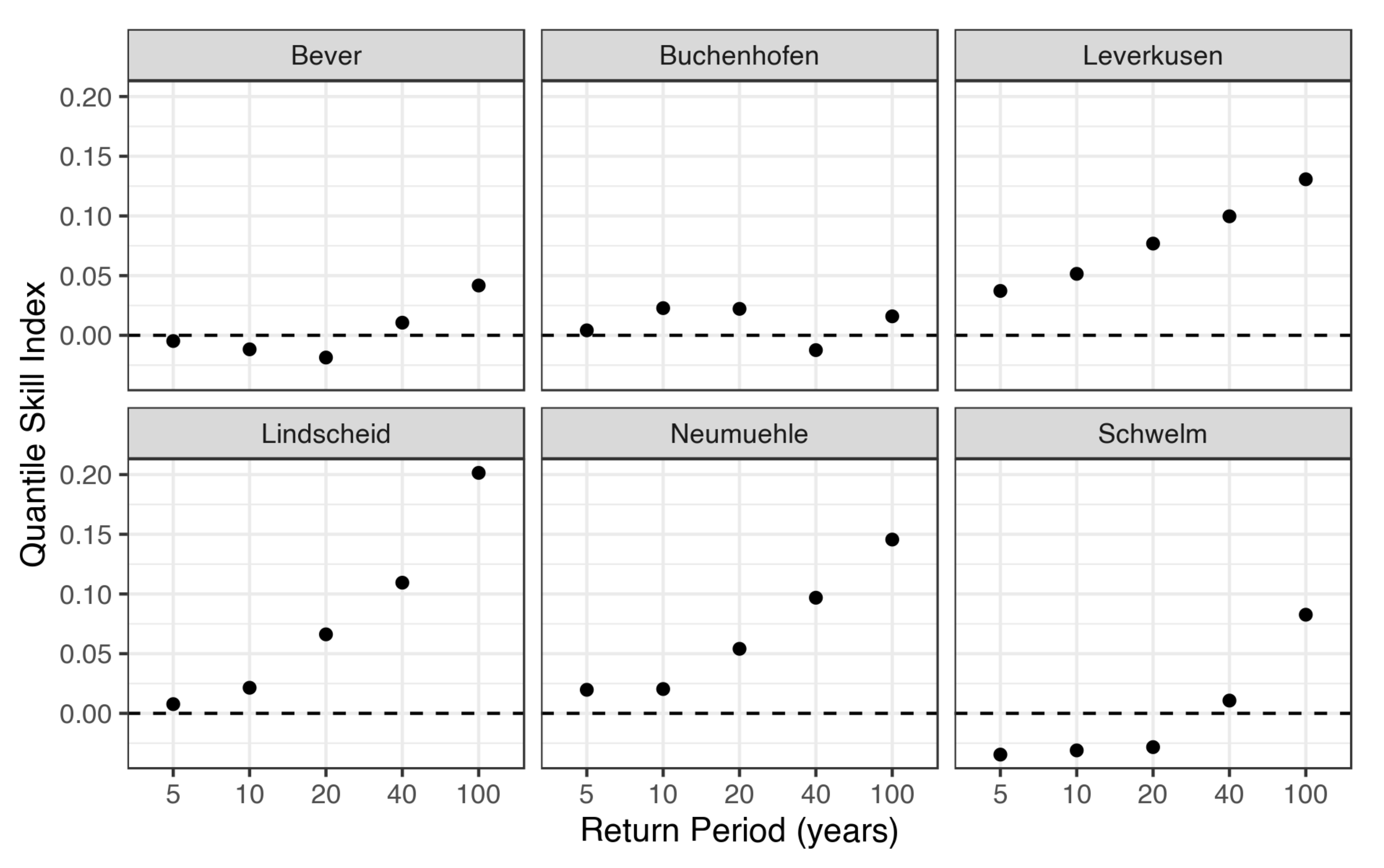
Figure 5 shows the cross-validated QSI evaluating the performance of the MS-GEV approach compared to the rd-GEV one. Similar behavior can be seen for all stations. For short return periods, the QSI is close to zero (denoting that both models are equally good), increasing towards longer periods. Station Lindscheid profits most from the MS-GEV with a 20% increase in skill for the 100-year return level. Only for a few points is skill negative, mostly for the shorter return periods.
3.1.4. Performance for Individual Durations
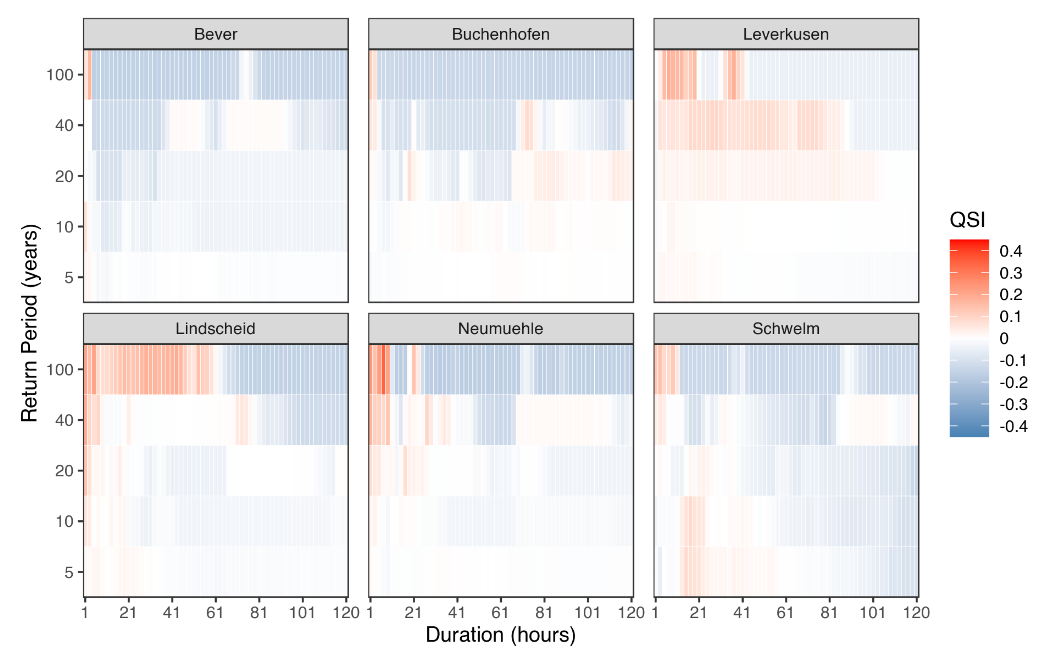
For a detailed comparison, we show the QSI conditioned on duration in Figure 6. The QSI varies appreciably over different durations for a given return period. For short durations (), the QSI is mostly positive for all return periods; for long durations , it is mostly negative. Gauge Lindscheid exhibits positive skill for many more combinations of durations () and return periods ; station Bever is the only station not showing a positive skill for very short durations, showing a general loss of skill for all but the shortest durations.
3.2. Simulation Study
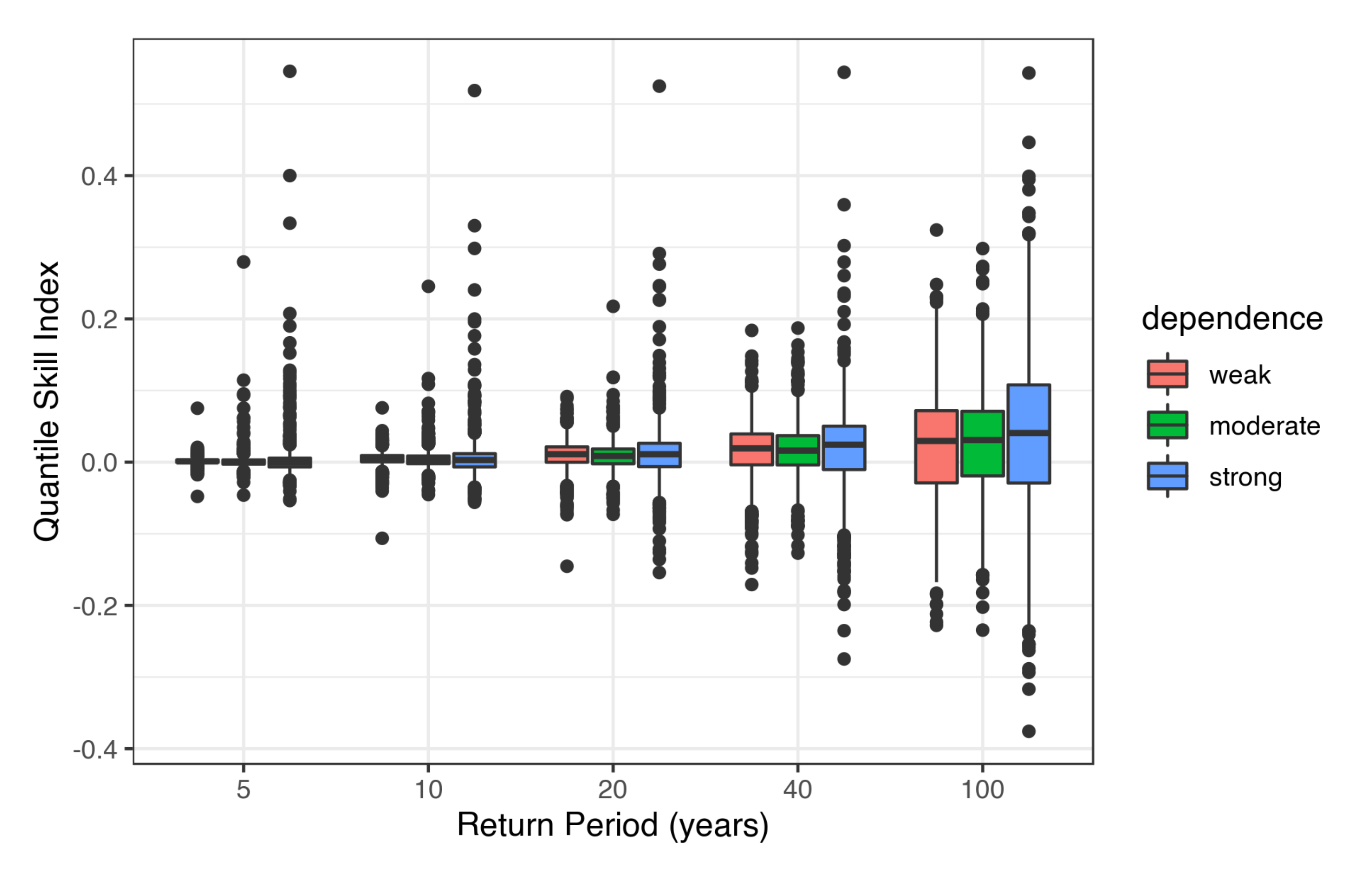
We studied the effect of the level of dependence on the performance of the MS-GEV approach. To this end, we used synthetic data with known dependence parameters ( and in Equation (8)) and estimate the performance for various levels of dependence. Figure 7 shows the cross-validated QSI obtained using Equation (17), using the averaged QS values over all durations for 1000 replications as box-whisker plots. Similar to the case study, the distance h used for the semivariogram of the Brown-Resnick process was the log-distance (Equation (10)).
The variation of skill among the replicates increases with increasing return period. The median is consistently positive (MS-GEV superior to rd-GEV) but below 0.05, suggesting that the dependence does not impact strongly on the performance results. The strong level of dependence leads to a slightly higher median skill but also to a considerable larger variance.
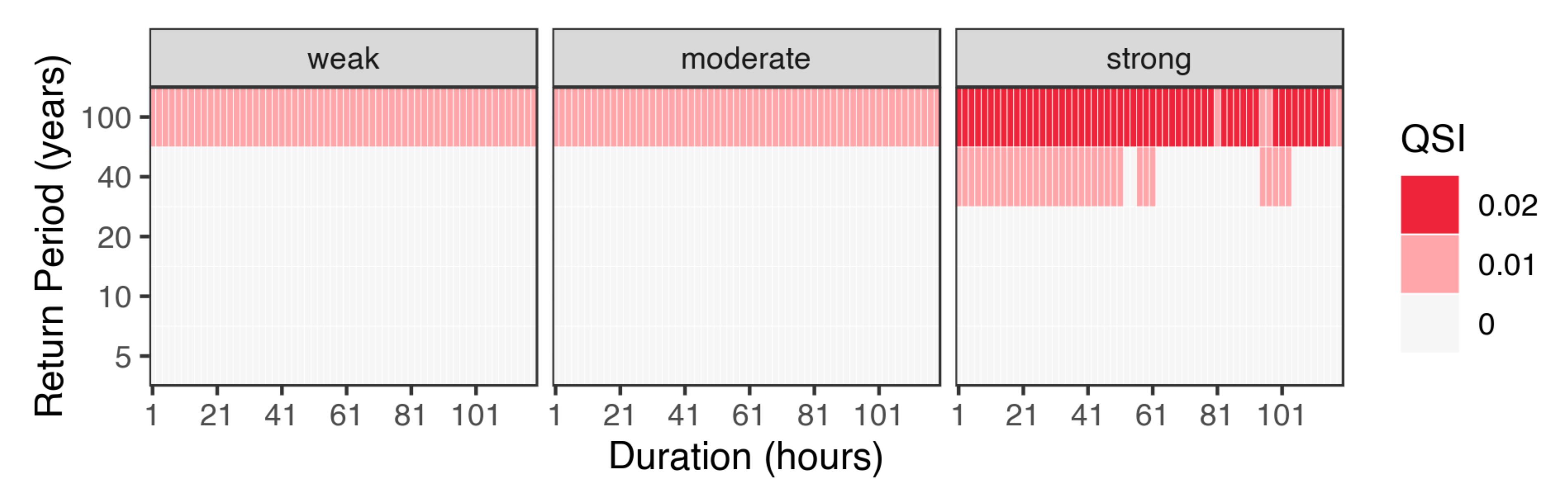
Figure 8 shows the QSI calculated with the model and reference QS averaged over all replicates for individual durations. The results are similar to the pooled QSI over all durations of Figure 7: The QSI increases with return period and dependence, staying below QSI = 0.1 for a 100 year return period and the strongly dependent series. This again suggests that the level of dependence has little impact on the performance of the return levels from the IDF curves.
4. Discussion
In this study, we obtained a measure of relative performance for return level estimates of IDF curves for various durations involving a max-stable process that allows for asymptotic dependence between durations (MS-IDF), compared to a model that assumes independence (rd-GEV). To do so, we built upon the previous study of Tyralis and Langousis [19], who focused on the theoretical basis of using max-stable processes for modeling IDF-curves and did not investigate the consequences in terms of model performance.
To investigate the possible impact of the asymptotical dependence, we evaluated and compared the performance of estimating IDF curves with two different approaches: i) using a max-stable process to describe the dependence between rainfall intensity maxima for different durations and ii) assuming independent maxima. We evaluated individual performance based on a score that allows us to focus on the tail of the distribution, namely the quantile score (QS). The comparison between the MS-GEV and rd-GEV approach was carried out with the quantile score index (QSI), an index based on the QS skill score. The QSI enables us to quantify a gain/loss in performance when accounting for asymptotic dependence in return level estimation.
The results of Figure 2 showed that the resulting pairwise extremal coefficient was non-isotropic when using the euclidean distance as the measure h in the semivariogram of the Brown-Resnick process for the MS-GEV approach. Thus, in contrast to the approach of Tyralis and Langousis [19], we explored the use of a logarithmic distance measure instead of an euclidean one for the semivariogram of the Brown-Resnick process. Figure 3 shows that this was a reasonable choice, with the resulting parametric extremal coefficient properly capturing the variability of the empirical extremal coefficient around its binned means.
A simulation study suggests a minor advantage of the MS-GEV approach over the rd-GEV, particularly for long return periods (large quantiles). This advantage increases with the strength of the dependence, but remains low (QSI ) even for the strongest level of dependence. A complementary case study for six gauges in the Wupper catchment (Germany) corroborates a general advantage for long return periods when averaging the performance measure over all durations. A detailed investigation of performance conditioned on durations shows, for our case study, that this advantage results mostly from short () and, in some cases, from intermediate () durations, depending, however, on the specific station.
The presented findings support the idea of Tyralis and Langousis [19] that max-stable processes are valuable models for IDF curve estimation. The simulation and case study results indicate that an increase in skill with the MS-GEV approach is mostly found for large quantiles and short to medium durations. This effect might be related to the fact that shorter durations have a larger number of pairs than the longer durations for the pairwise likelihood. This means that the longer durations could be underrepresented in the current likelihood expression, leading to a better fit of the model for the shorter durations for the MS-GEV approach. However, extreme events of short durations have usually a higher impact on society than those of long durations. Therefore, we believe that this underrepresentation does not necessarily detract value from using the MS-GEV approach. When focusing on large quantiles and short durations, it might be worth taking the added computational expense and model complexity in exchange for increased skill in the return levels for such events.
In addition, the simulation study demonstrated that the level of dependence had a modest impact on the overall performance and variability of the MS-GEV approach. These findings contradict those of Zheng et al. [25], who found that the dependence strength did not influence the performance of the return level estimates. However, our study focused on a different dependence structure than that of Zheng et al. [25], who used a spatial approach, in contrast to our duration space. This contradiction may be associated with the particular form of the asymptotic dependence for the different durations of , which stems from the nature of as random ordered variables. As previously studied by [20,42], when two random variables are intrinsically ordered, each margin’s distribution is affected, something that has to be taken into account. While the response surfaces described in Equations (12) and (13) take this ordering into account, the dependence structure given in Equation (8) does not, a factor that could explain the contradiction with previous studies.
The parametric estimate of the extremal coefficient from the MS-GEV approach shown in Figure 3 appears to be a reasonable fit for the empirical values of when the ratio of the duration pair is around (). However, as the upper duration gets around six times larger than the lower duration, the model consistently overestimates the strength of the dependence. Figure 3 also showed that duration pairs involving short lower durations had an extremal coefficient that approached independence (i.e., ) faster than those with longer lower durations as increased. This suggests that the dependence between rainfall maxima of different aggregation durations is short-ranged, in particular, for the shorter durations.
For an operational use of this approach, uncertainty estimates for the quantiles (IDF curves) need to be incorporated. In this regard, Ganguli and Coulibaly [12], Mélese et al. [43] showed that a Bayesian Hierarchical Model approach resulted in reliable credibility intervals for IDF curves. For the rd-GEV approach, we investigate a bootstrap-based method for estimating the uncertainty of d-GEV based return levels in a different study [9]. We also limited our study to using data with hourly frequency, resulting in the value of the (sub-hourly) parameter of the d-GEV to be artificially set to zero (what we called the rd-GEV). Further studies would benefit from using sub-hourly frequencies, allowing to vary freely. Moreover, we assumed that the stations’ data was stationary, ignoring the possible effects of climate change. Several studies have shown that accounting for nonstationarity has a measurable effect on the return levels estimates [11,12,13].
The method presented in this study is a straightforward and practical manner of estimating IDF return level performance based on a max-stable process. The results for the case study encourage to investigate its performance within a larger geographical setting. Furthermore, it seems worth implementing more flexible functions describing the variability of GEV parameters with duration as used for the response surface, e.g., an additional parameter accounting for different behavior, particularly for short durations, as suggested in Koutsoyiannis et al. [5]. Another critical issue for future studies is to explore how different dependence structures could impact the performance of the estimation. Furthermore, a comparison with the recent developments in the use of covariates for the rd-GEV approach could result in better skill for such an approach compared with our current MS-GEV one [9].
5. Conclusions
Our findings indicate that the use of models that allow for the asymptotic dependence between rainfall maxima of different durations when estimating IDF curves can lead to moderately better return level estimates, particularly for long return periods (100 years, generally of considerable interest) and short durations (). However, the former comes at the expense of the added complexity of modeling the asymptotic dependence. Furthermore, this asymptotical dependence seems to be short-ranged for the short durations. We, therefore, recommend the use of the simpler univariate-EVT methods assuming independence between durations for a single station when the main goal is obtaining return levels for a wide range of short and long durations from IDF-curves.
Author Contributions
Conceptualization, O.E.J. and H.W.R.; Data curation, M.S.; Formal analysis, O.E.J. and H.W.R.; Funding acquisition, H.W.R.; Investigation, O.E.J.; Methodology, O.E.J. and J.U.; Project administration, H.W.R.; Resources, H.W.R.; Software, O.E.J. and J.U.; Supervision, H.W.R.; Validation, O.E.J.; Visualization, O.E.J.; Writing—original draft, O.E.J.; Writing—review & editing, J.U., M.S. and H.W.R., please turn to the CRediT taxonomy for the term explanation. All authors have read and agreed to the published version of the manuscript.
Funding
The research was partially supported by Deutsche Forschungsgemeinschaft (DFG) through grant CRC 1114 “Scaling Cascades in Complex Systems,” Project A01 “Coupling a multiscale stochastic precipitation model to large scale flow.” O.E.J. acknowledges support by the Mexican National Council for Science and Technology (CONACyT) and the German Academic Exchange Service (DAAD). J.U. and O.E.J. acknowledge support by Deutsche Forschungsgemeinschaft (DFG) within the research training program NatRiskChange (GRK 2043/1). The publication of this article was funded by Freie Universität Berlin.
Acknowledgments
We would like to acknowledge the Wupperverband (Untere Lichtenplatzer Str. 100, 42289 Wuppertal, North Rhine-Westphalia, Germany) for providing the precipitation time series. We also acknowledge the contribution of Hans Van de Vyver on the use of the log-distance for the variogram.
Conflicts of Interest
The authors declare no conflict of interest.
Abbreviations
The following abbreviations are used in this manuscript:
| IDF | Intensity-Duration-Frequency (curve) |
| GEV | Generalized Extreme Value distribution |
| d-GEV | Duration-dependent GEV |
| rd-GEV | Reduced d-GEV-based approach for modeling IDF curves |
| MS-GEV | Max-stable-based approach for modeling IDF curves |
| QS | Quantile Score |
| QSS | Quantile Skill Score |
| QSI | Quantile Skill Index |
Appendix A. Inference from the Brown-Resnick Max-Stable Process
Consider a stochastic process , where is a compact subset of , and a Poisson process with intensity on . Let be independent realizations of a process with , and let be points of the Poisson process. A simple max-stable process is then given by
Smith [44] proposed a useful analogy to interpret this kind of max-stable process as the so-called rainfall-storms interpretation. In this interpretation, represents the overall intensity of a rainfall storm that impacts the region , and corresponds to the total amount of rainfall for the storm centered at position d. A max-stable process would then be the pointwise maxima (taken over each point in ) over an infinite number of storms.
For the Brown-Resnick process, we follow the proposal from Kabluchko et al. [33], where . Here, is a Gaussian process with stationary increments and semivariogram . The bivariate density function for the Brown-Resnick process [17,33], is
where follows a unit Fréchet distribution, denotes the standard normal distribution function, h is a measure of the “distance” between duration pairs (given in this study by Equation 10), and the semivariogram is defined in Equation (8).
For inference purposes, we applied the commonly used pairwise likelihood proposed by Padoan et al. [45], given by
where represents the parameters to estimate, and each term is the (appropriately transformed) bivariate density function derived from Equation (A2) for observed maxima at durations and . Note that the first three parameters in are the univariate parameters of the GEV distribution, unique for each duration, while the last two parameters of are the parameters of the Brown-Resnick process, which model the asymptotic dependence.
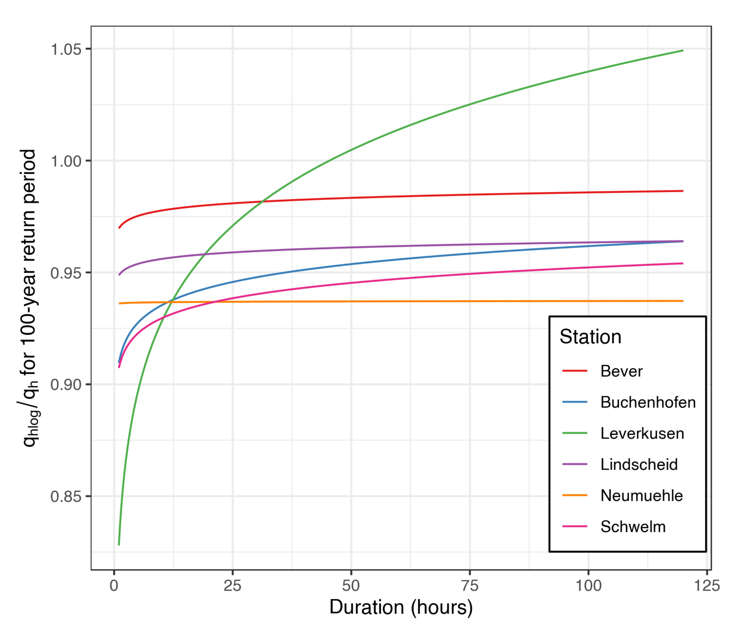
Appendix B. Comparison of 100-year Return Level between Euclidean and Log-Distance for MS-GEV Approach
Figure A1 shows a comparison of the resulting 100-year return level intensity resulting from the MS-GEV approach using the euclidean distance and the log-distance . To facilitate the comparison, it shows the ratio , where is the quantile corresponding to the probability of 0.99, that is, the corresponding 100-year return level.
Figure A1.
Comparison of the 100-year return level intensity for the MS-GEV approach using the euclidean distance and the log-distance .
Figure A1.
Comparison of the 100-year return level intensity for the MS-GEV approach using the euclidean distance and the log-distance .

Surprisingly, although the variability of around its mean is remarkably different when using instead of , the resulting 100-year return levels are very similar for both distances. The single exception was for station Leverkusen, which is the only station of the catchment located in the Upper Rhine Plain; the change observed for this stations was however still relatively small. However, this result is only accounting for the point estimates of the return levels. As seen in Figure 2 and Figure 3, the variability of the extremal dependence is much higher when using the euclidean distance than the log-distance . Thus, we believe that the resulting uncertainty for the MS-GEV approach should be lower when using instead of . Nevertheless, as mentioned in the limitations of our study, we did not perform any estimation of the uncertainty.
Appendix C. QQ-Plots for Selected Stations and Durations
Figure A2 shows the QQ-plots for validation of the marginal fits of the GEV distribution for four intensity maxima series , with , for three stations (Bever, Leverkusen, and Neumuehle.). The closer that the points are aligned to the identity line, the better the fit of the GEV distribution.
Figure A2.
QQ plots for model checking of the marginal distributions for three stations: Bever (top row), Leverkusen (middle row), and Neumuehle (bottom row). The duration used for the accumulation of the rainfall maxima is indicated in each plot.
Figure A2.
QQ plots for model checking of the marginal distributions for three stations: Bever (top row), Leverkusen (middle row), and Neumuehle (bottom row). The duration used for the accumulation of the rainfall maxima is indicated in each plot.

References
- Chow, V.T. Frequency analysis of hydrologic data with special application to rainfall intensities. Univ. Ill. Bull. 1953, 50, 86. [Google Scholar]
- Aparicio, F. Fundamentos de Hidrología de Superficie Fundamentals of Surface Hydrology; Limusa: Balderas, Mexico, 1997; pp. 168–176. [Google Scholar]
- García-Bartual, R.; Schneider, M. Estimating Maximum Expected Short-Duration Convective Storms. Phys. Chem. Earth Part B 2001, 26, 675–681. [Google Scholar] [CrossRef]
- Monjo, R. Measure of rainfall time structure using the dimensionless n-index. Clim. Res. 2016, 67, 71–86. [Google Scholar] [CrossRef] [Green Version]
- Koutsoyiannis, D.; Kozonis, D.; Manetas, A. A mathematical framework for studying rainfall intensity-duration-frequency relationships. J. Hydrol. 1998, 206, 118–135. [Google Scholar] [CrossRef]
- Lehmann, E.A.; Phatak, A.; Stephenson, A.G.; Lau, R. Spatial modelling framework for the characterisation of rainfall extremes at different durations and under climate change. Environmetrics 2016, 27, 239–251. [Google Scholar] [CrossRef] [Green Version]
- Van de Vyver, H. A multiscaling-based intensity–duration–frequency model for extreme precipitation. Hydrol. Process. 2018, 32, 1635–1647. [Google Scholar] [CrossRef]
- Ritschel, C.; Ulbrich, U.; Nevir, P.; Rust, H.W. Precipitation extremes on multiple timescales—Bartlett-Lewis rectangular pulse model and intensity-duration-frequency curves. Hydrol. Earth Syst. Sci. 2017, 21, 6501–6517. [Google Scholar] [CrossRef] [Green Version]
- Ulrich, J.; Jurado, O.E.; Peter, M.; Scheibel, M.; Rust, H.W. Estimating IDF curves consistently over durations with spatial covariates. Water 2020, 12, 3119. [Google Scholar] [CrossRef]
- Fischer, M.; Rust, H.; Ulbrich, U. A spatial and seasonal climatology of extreme precipitation return-levels: A case study. Spat. Stat. 2019, 34. [Google Scholar] [CrossRef]
- Padulano, R.; Reder, A.; Rianna, G. An ensemble approach for the analysis of extreme rainfall under climate change in Naples (Italy). Hydrol. Process. 2019, 33, 2020–2036. [Google Scholar] [CrossRef]
- Ganguli, P.; Coulibaly, P. Does nonstationarity in rainfall require nonstationary intensity-duration-frequency curves? Hydrol. Earth Syst. Sci. 2017, 21, 6461–6483. [Google Scholar] [CrossRef] [Green Version]
- Ganguli, P.; Coulibaly, P. Assessment of future changes in intensity-duration-frequency curves for Southern Ontario using North American (NA)-CORDEX models with nonstationary methods. J. Hydrol.-Reg. Stud. 2019, 22. [Google Scholar] [CrossRef]
- Muller, A.; Bacro, J.N.; Lang, M. Bayesian comparison of different rainfall depth-duration-frequency relationships. Stoch. Environ. Res. Risk Assess. 2008, 22, 33–46. [Google Scholar] [CrossRef] [Green Version]
- Van de Vyver, H. Bayesian estimation of rainfall intensity-duration-frequency relationships. J. Hydrol. 2015, 529, 1451–1463. [Google Scholar] [CrossRef]
- Singh, V.P.; Zhang, L. IDF curves using the Frank Archimedean copula. J. Hydrol. Eng. 2007, 12, 651–662. [Google Scholar] [CrossRef]
- Davison, A.C.; Huser, R.; Thibaud, E. Geostatistics of Dependent and Asymptotically Independent Extremes. Math. Geosci. 2013, 45, 511–529. [Google Scholar] [CrossRef] [Green Version]
- Stephenson, A.G.; Lehmann, E.A.; Phatak, A. A max-stable process model for rainfall extremes at different accumulation durations. Weather Clim. Extrem. 2016, 13, 44–53. [Google Scholar] [CrossRef] [Green Version]
- Tyralis, H.; Langousis, A. Estimation of intensity–duration–frequency curves using max-stable processes. Stoch. Environ. Res. Risk Assess. 2019, 33, 239–252. [Google Scholar] [CrossRef]
- Nadarajah, S.; Anderson, C.W.; Tawn, J.A. Ordered multivariate extremes. J. R. Stat. Soc. Ser. B Stat. Methodol. 1998, 60, 473–496. [Google Scholar] [CrossRef]
- Coles, S. An Introduction to Statistical Modeling of Extreme Values; Springer: London, UK, 2001. [Google Scholar] [CrossRef]
- Ulrich, J.; Ritschel, C. IDF: Estimation and Plotting of IDF Curves; R Package Version 2.0.0; R Package: Madison, WI, USA, 2020. [Google Scholar]
- Ribatet, M. Spatial extremes: Max-stable processes at work. J. Société Française Stat. Rev. Stat. Appl. 2013, 154, 156–177. [Google Scholar]
- De Haan, L. A Spectral Representation for Max-Stable Processes. Ann. Probab. 1984, 12, 1194–1204. [Google Scholar]
- Zheng, F.; Thibaud, E.; Leonard, M.; Westra, S. Assessing the performance of the independence method in modeling spatial extreme rainfall. Water Resour. Res. 2015, 51, 7744–7758. [Google Scholar] [CrossRef]
- Dey, D.K.; Yan, J. Extreme Value Modeling and Risk Analysis: Methods and Applications; CRC: New York, NY, USA, 2016. [Google Scholar]
- Engelke, S.; Malinowski, A.; Kabluchko, Z.; Schlather, M. Estimation of Hüsler-Reiss distributions and Brown-Resnick processes. J. R. Stat. Soc. Ser. B Stat. Methodol. 2015, 77, 239–265. [Google Scholar] [CrossRef] [Green Version]
- Thibaud, E.; Aalto, J.; Cooley, D.S.; Davison, A.C.; Heikkinen, J. Bayesian inference for the brown-resnick process, with an application to extreme low temperatures. Ann. Appl. Stat. 2016, 10, 2303–2324. [Google Scholar] [CrossRef]
- Asadi, P.; Davison, A.C.; Engelke, S. Extremes on river networks. Ann. Appl. Stat. 2015, 9, 2023–2050. [Google Scholar] [CrossRef]
- Davison, A.C.; Padoan, S.A.; Ribatet, M. Statistical Modeling of Spatial Extremes. Stat. Sci. 2012, 27, 161–186. [Google Scholar] [CrossRef] [Green Version]
- Buhl, S.; Klüppelberg, C. Anisotropic Brown-Resnick space-time processes: Estimation and model assessment. Extremes 2016, 19, 627–660. [Google Scholar] [CrossRef] [Green Version]
- Cooley, D.; Cisewski, J.; Erhardt, R.J.; Jeon, S.; Mannshardt, E.; Omolo, B.O.; Sun, Y. A survey of spatial extremes: Measuring spatial dependence and modeling spatial effects. Revstat Stat. J. 2012, 10, 135–165. [Google Scholar]
- Kabluchko, Z.; Schlather, M.; de Haan, L. Stationary max-stable fields associated to negative definite functions. Ann. Probab. 2009, 37, 2042–2065. [Google Scholar] [CrossRef]
- Van de Vyver, H.; Van den Bergh, J. The Gaussian copula model for the joint deficit index for droughts. J. Hydrol. 2018, 561, 987–999. [Google Scholar] [CrossRef]
- Ribatet, M. SpatialExtremes: Modelling Spatial Extremes; R Package Version 2.0-8; R Package: Madison, WI, USA, 2020. [Google Scholar]
- Marcon, G.; Padoan, S.A.; Naveau, P.; Muliere, P.; Segers, J. Multivariate nonparametric estimation of the Pickands dependence function using Bernstein polynomials. J. Stat. Plan. Inference 2017, 183, 1–17. [Google Scholar] [CrossRef] [Green Version]
- Vettori, S.; Huser, R.; Genton, M.G. A comparison of dependence function estimators in multivariate extremes. Stat. Comput. 2018, 28, 525–538. [Google Scholar] [CrossRef] [Green Version]
- R Core Team. R: A Language and Environment for Statistical Computing; R Foundation for Statistical Computing: Vienna, Austria, 2020. [Google Scholar]
- Bentzien, S.; Friederichs, P. Decomposition and graphical portrayal of the quantile score. Q. J. R. Meteorol. Soc. 2014, 140, 1924–1934. [Google Scholar] [CrossRef]
- Wilks, D.S. Chapter 9—Forecast Verification. In Statistical Methods in the Atmospheric Sciences; Elsevier: Amsterdam, The Netherlands, 2019; pp. 369–483. [Google Scholar] [CrossRef]
- Hastie, T.; Tibshirani, R.; Friedman, J. Elements of Statistical Learning, 2nd ed.; Springer: Berlin, Germany, 2009. [Google Scholar] [CrossRef]
- Nadarajah, S.; Afuecheta, E.; Chan, S. Ordered random variables. Opsearch 2019, 56, 344–366. [Google Scholar] [CrossRef]
- Mélèse, V.; Blanchet, J.; Molinié, G. Uncertainty estimation of Intensity–Duration–Frequency relationships: A regional analysis. J. Hydrol. 2018, 558, 579–591. [Google Scholar] [CrossRef] [Green Version]
- Smith, R.L. Max-stable processes and spatial extremes. Unpublished Manuscripts. 1990. Available online: http://www.rls.sites.oasis.unc.edu/postscript/rs/spatex.pdf (accessed on 25 November 2020).
- Padoan, S.A.; Ribatet, M.; Sisson, S.A. Likelihood-based inference for max-stable processes. J. Am. Stat. Assoc. 2010, 105, 263–277. [Google Scholar] [CrossRef]
Figure 1.
Left: (Lower panel) Distribution of the annual rainfall maxima at a 1-h accumulation duration plotted against time. Each boxplot shows the distribution of the pooled maxima from the six stations used for the case study in the Wupper catchment region. (Upper panel) Time series of the annual rainfall maxima, showing the values of each station as a different color. Right: Map of the Wupper catchment (dashed line) showing the location of all 6 stations; the lower-right corner shows the location of the catchment within Germany.

Figure 2.
Nonparametric (dots = ) and parametric (solid line = ) estimates for the pairwise extremal coefficient using the euclidean distance . The estimated nonparametric mean of for each duration lag bin is shown as black dots. Each color represents the lower duration used for each duration pair.
Figure 2.
Nonparametric (dots = ) and parametric (solid line = ) estimates for the pairwise extremal coefficient using the euclidean distance . The estimated nonparametric mean of for each duration lag bin is shown as black dots. Each color represents the lower duration used for each duration pair.

Figure 3.
Nonparametric (dots = ) and parametric (solid line = ) estimates for the pairwise extremal coefficient using the logarithmic distance . For ease of interpretation, the values of the log-distance in the x-axis were transformed to the duration ratio . The estimated nonparametric mean of for each duration ratio bin is shown as black dots. Each color represents the lower duration used for each duration pair. Notice the difference in the variability of the point clouds when compared to those of Figure 2.

Figure 4.
Comparison of IDF curves for the MS-GEV (solid line) and rd-GEV approach (dashed line) for all stations. Different colors represent different return periods; from bottom to top: (5, 10, 20, 40, 100) years.
Figure 4.
Comparison of IDF curves for the MS-GEV (solid line) and rd-GEV approach (dashed line) for all stations. Different colors represent different return periods; from bottom to top: (5, 10, 20, 40, 100) years.

Figure 5.
Quantile Skill Index comparing the MS-GEV versus the rd-GEV approach for all stations in the Wuppertal catchment. Positive values favor the MS-GEV approach.
Figure 5.
Quantile Skill Index comparing the MS-GEV versus the rd-GEV approach for all stations in the Wuppertal catchment. Positive values favor the MS-GEV approach.

Figure 6.
Quantile Skill Index conditioned on duration comparing the MS-GEV (using log-distance ) versus the rd-GEV approach for all stations in the Wuppertal catchment. Positive values favor the MS-GEV approach for different durations.
Figure 6.
Quantile Skill Index conditioned on duration comparing the MS-GEV (using log-distance ) versus the rd-GEV approach for all stations in the Wuppertal catchment. Positive values favor the MS-GEV approach for different durations.

Figure 7.
Quantile Skill Index calculated from QS averaged for all durations , comparing the MS-GEV versus the rd-GEV approach as a function of simulated data’s dependence parameter. Positive values of the QSI favor the MS-GEV approach. Each boxplot represents the distribution from the results of 1000 simulations.

Figure 8.
Quantile Skill Index, as in Figure 7, but showing the quantile score index (QSI) as a function of return period and duration.
Figure 8.
Quantile Skill Index, as in Figure 7, but showing the quantile score index (QSI) as a function of return period and duration.


Table 1.
Parameter estimates from the MS-GEV approach for stations in the Wupper catchment using durations .
Table 1.
Parameter estimates from the MS-GEV approach for stations in the Wupper catchment using durations .
| Station | c | |||||
|---|---|---|---|---|---|---|
| Bever | 1.42 | 2.09 | 13.32 | 2.84 | 0.03 | −0.58 |
| Buchenhofen | 1.39 | 2.22 | 13.38 | 3.03 | 0.02 | −0.63 |
| Leverkusen | 1.32 | 2.19 | 10.74 | 2.34 | 0.05 | −0.64 |
| Lindscheid | 1.54 | 2.44 | 13.69 | 3.23 | 0.06 | −0.64 |
| Neumuehle | 1.54 | 1.84 | 13.52 | 2.74 | 0.04 | −0.60 |
| Schwelm | 1.53 | 1.74 | 13.07 | 2.77 | 0.05 | −0.62 |
Publisher’s Note: MDPI stays neutral with regard to jurisdictional claims in published maps and institutional affiliations. |
© 2020 by the authors. Licensee MDPI, Basel, Switzerland. This article is an open access article distributed under the terms and conditions of the Creative Commons Attribution (CC BY) license (http://creativecommons.org/licenses/by/4.0/).
Share and Cite
MDPI and ACS Style
Jurado, O.E.; Ulrich, J.; Scheibel, M.; Rust, H.W. Evaluating the Performance of a Max-Stable Process for Estimating Intensity-Duration-Frequency Curves. Water 2020, 12, 3314. https://doi.org/10.3390/w12123314
AMA Style
Jurado OE, Ulrich J, Scheibel M, Rust HW. Evaluating the Performance of a Max-Stable Process for Estimating Intensity-Duration-Frequency Curves. Water. 2020; 12(12):3314. https://doi.org/10.3390/w12123314
Chicago/Turabian StyleJurado, Oscar E., Jana Ulrich, Marc Scheibel, and Henning W. Rust. 2020. "Evaluating the Performance of a Max-Stable Process for Estimating Intensity-Duration-Frequency Curves" Water 12, no. 12: 3314. https://doi.org/10.3390/w12123314
Note that from the first issue of 2016, this journal uses article numbers instead of page numbers. See further details here.