3D Ensemble Simulation of Seawater Temperature – An Application for Aquaculture Operations

Introduction

Fish currently supplies 17% of the protein consumed worldwide (Martin et al., 2016). The current demand for fish is much higher than what could be supplied by marine fish catch alone (Merino et al., 2012). These pressures put wild fish and other aquatic organisms at risk of overfishing. These facts signify the importance of developing new aquaculture facilities for seafood production. Already half of the fish production in the world comes from aquaculture (FAO, 2020). Efforts are being made to ensure a continuous and reliable supply of good quality seafood. These efforts encourage the setting up of new fisheries and aquaculture facilities around the world (FAO, 2020). But for sustainable seafood production, necessary management practices should be in place. This includes continuous monitoring and maintenance of the seawater quality, fish health, growth, as well as disease monitoring. Environmental considerations for farming operations are temperature, salinity and dissolved oxygen among others. For operational decision making in aquaculture farms, temperature is an important environmental property (Hurst, 2007; Ibarz et al., 2010; Besson et al., 2016; Masroor et al., 2018). Fish species have tolerance levels of temperature and beyond these tolerance levels, fish growth and health are adversely impacted (Berlinsky et al., 2007; Llorente and Luna, 2013; Balbuena-Pecino et al., 2019). At such scenarios, to run the farm business profitably, appropriate measure needs to be taken related to operations (Besson et al., 2016; Hobday et al., 2016). For example, low water temperature may cause problems such as low food intake, reduced growth and even mortality in extreme scenarios requiring lower food feeding (Hurst, 2007). High temperatures in summer results in oxygen constraint in the fish cages, since at higher temperatures water does not hold enough oxygen. This demands a low stock of fish to avoid fish mortality resulting in economic loss (Besson et al., 2016). These threshold seawater temperatures, whose information is beneficial to the aquaculture farmers, are different for different species. Therefore, seawater temperature is a main guiding variable which farmers rely on and for this reason it is selected for further study in this research. Several studies have been conducted in the past to correlate the fish growth and health with water temperature (Person-Le Ruyet et al., 2004; Berlinsky et al., 2007; Mayer et al., 2008; Ibarz et al., 2010).

Water properties are simulated and forecasted in real-time in many sectors using hydrodynamic and water quality modeling (Vandenbulcke and Barth, 2015; Chaudhuri et al., 2016; Lima et al., 2019; Pesce et al., 2019). These simulated information benefits the farmer to plan the short and long-term operations of the farms well in advance. For example, increasing water temperature may result in a higher growth rate for some farmed fish species but extremely high seawater temperatures lead to a greater chance of disease outbreaks and algal blooms in certain regions (Lorentzen, 2008). It is the preparedness of the farming community which could help them benefit from thermal changes and/or minimize any negative impact of it (Callaway et al., 2012; Merino et al., 2012; Bell et al., 2013).

Simulation results from numerical models, for example, of past events can be useful in preparing a suite of scenario-based decisions, which can be used as a guideline to ensure efficient management in aquaculture. However, uncertainties in the model inputs and forcing, such as atmospheric forcing, as well as inaccurate model parameterization lead to an uncertain numerical simulation of water quality variables, which may lead to wrong decisions. A deterministic model utilizes a single set of inputs and model parameters yielding a single model output which is a best guess with a false sense of certainty. A deterministic simulation therefore has no consideration for the uncertainties that are inherent in the atmospheric forcing fields, boundary information or model parameters (Chaudhuri et al., 2016). In this context, probabilistic simulation methods offer greater advantages. The advantage of these methods over a single deterministic simulation is that it does not predict the most likely event, instead predicts all possible events (Buizza, 2018). This, when seen in the context of aquaculture, gives end-users a greater benefit as it provides more complete future scenarios and the likelihood of certain events. Probabilistic information of extreme scenarios, such as extreme seawater temperature (SWT), has significant impact on various decisions that are to be made in an aquaculture farm. These include changes in the sea cage depth, changes in the fish stocking density, changes in feed ratios and disease control mechanisms. All likely events and a measure of their probability would enable informed decision-making and help to increase the confidence of decision-makers in the forecasted information (Vandenbulcke and Barth, 2015). Apart from this, the consistency in the simulations from an ensemble method is proven to be higher compared to deterministic simulations (Buizza, 2018). Studies have shown that the additional information reflecting the uncertainties available in the ensemble simulation have higher economic value to the user than a single deterministic simulation (Richardson, 2000).

There is a general lack studies on quantifying uncertainties in SWT simulations applied anywhere in the Mediterranean Sea despite tremendous growth potential for aquaculture in the region. Lack of uncertainty estimate puts decision making in the aquaculture at risk due to rapid changes in the climate and marine environment. Such changes require adequate response in the planning and operations of farms. By developing an ensemble model and providing three dimensional probabilistic estimates of the SWT, we intend to support aquaculture operations in making informed decisions. With the existing methodologies of quantifying uncertainties, we assess the seasonal, spatial and vertical gradient of SWT fluctuations which enables the appropriate operational changes in the aquaculture farms.

Study Area

General Information: Aegean Sea

The Aegean Sea is a part of the Eastern Mediterranean Sea. It is shared by two countries, Greece and Turkey. The characteristic feature of this sea is that it is dotted with numerous islands and highly irregular coastline. Due to its complex bathymetry, semi-isolated deep basins could be seen in the Aegean Sea, making it complex in terms of seawater circulation. Its flow is a combination of wind-driven and thermohaline-driven flow. It also features complex mesoscale eddy fields (Olson et al., 2007). The South Aegean Sea and its adjacent seas show a circular pattern from surface down to intermediate layers. This shows significant synoptic to inter-annual variability. In general, cyclonic circulations are observed along the eastern and western coastline of the Southern Aegean Sea. There is also inter-sea exchange of waters from the neighboring seas through Cretan Arc Straits (Kassis et al., 2016).

Aquaculture in Greece

Favorable climatic and environmental conditions, a long coastline, historical experience, and scientific know-how have given Greece advantage over other European countries in terms of aquaculture. Therefore, the coastline of Greece is dotted with aquaculture farms across the country. At present this sector represents a major portion of the total seafood production in Greece¹. In Greece, commonly farmed species are finfish (seabream and seabass) and shellfish (mussels). Cage based coastal aquaculture is the most popular form of aquaculture. These cages are located strategically to utilize natural water circulation and to safeguard against severe weather conditions. Land-based breeding stations supply the fry to these cages facilities where fish is farmed for 12–24 months. Generally, fish is harvested at a weight range of 350–450 g. This also depends on the local water temperature (FAO, 2011). For this study, two aquaculture sites are selected namely Ortholithi (37° 21′ 2.52′′ N 22° 47′ 58.38′′ E) and Ovrios (37° 51′ 27.57′′ N 23° 8′ 45.60′′ E) (Figure 1). Ortholithi is located on the mainland shorelines in the Argolic Gulf, whereas Ovrios is an island in the Saronic Gulf. Both farms are in water depths ranging from 40 m to 80 m. The two gulf areas are unique in their bathymetry. While the Saronic Gulf is a shallow area of around 200 m depth, the Argolic Gulf hosts deep sea trench with depths up to 800 m (Figure 3). The cage depth, which is measured as distance between water surface and the bottom of the cage is 10 m in both cases. Both circular and rectangular variants of the cages are used. The surface dimension of individual cages differ within the same farm. Usually the surface area of cages is 15–20 m in diameter for a cage depth of 10 m. Farms at Ortholithi and Ovrios occupy area of ∼34,000 m² and ∼20,000 m² respectively. In both sites, European Seabream (Sparus aurata) species is farmed. These two farms are operated by a Greek aquaculture company, Selonda. Continuous temperature and oxygen monitoring are carried out at the farms for operational purposes. These data are provided by Selonda for model validation purposes.

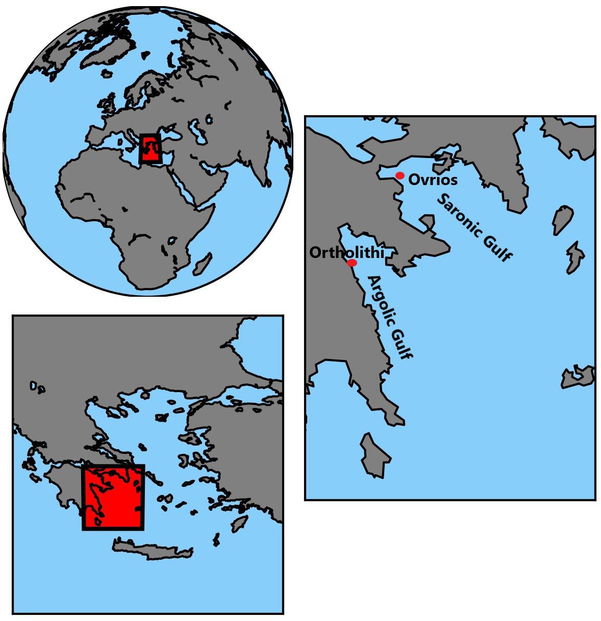
Figure 1. Location of the study area with two Gulf areas and two observation points – Ortholithi and Ovrios.

Data and Methods

In order to support the decision making of aquaculture operators, this study proposes a methodology to produce three-dimensional seawater temperature fields with associated atmospheric uncertainty using a numerical modeling tool. The materials and methodological steps included are as shown in Figure 2. These steps are detailed in the following sections. First, we describe the datasets that are used to develop the model in section “Data.” Section “Methods” elaborates on the various steps involved in model setup. In section “Verification measures,” various verification measures that are used to compare the performance of deterministic and ensemble simulations are described. In the final section “Uncertainty analysis,” the methods of uncertainty analysis are described.

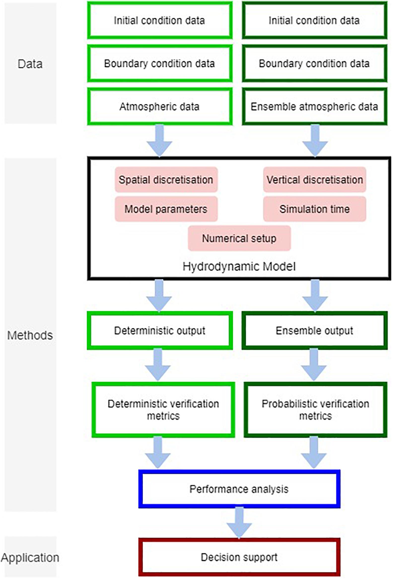
Figure 2. Methodological framework consists three major components – Data, Methods, and Application. There are two main models setups that are followed. Left side track (light green) represents the deterministic model and the right side track (dark green) represent the ensemble model.

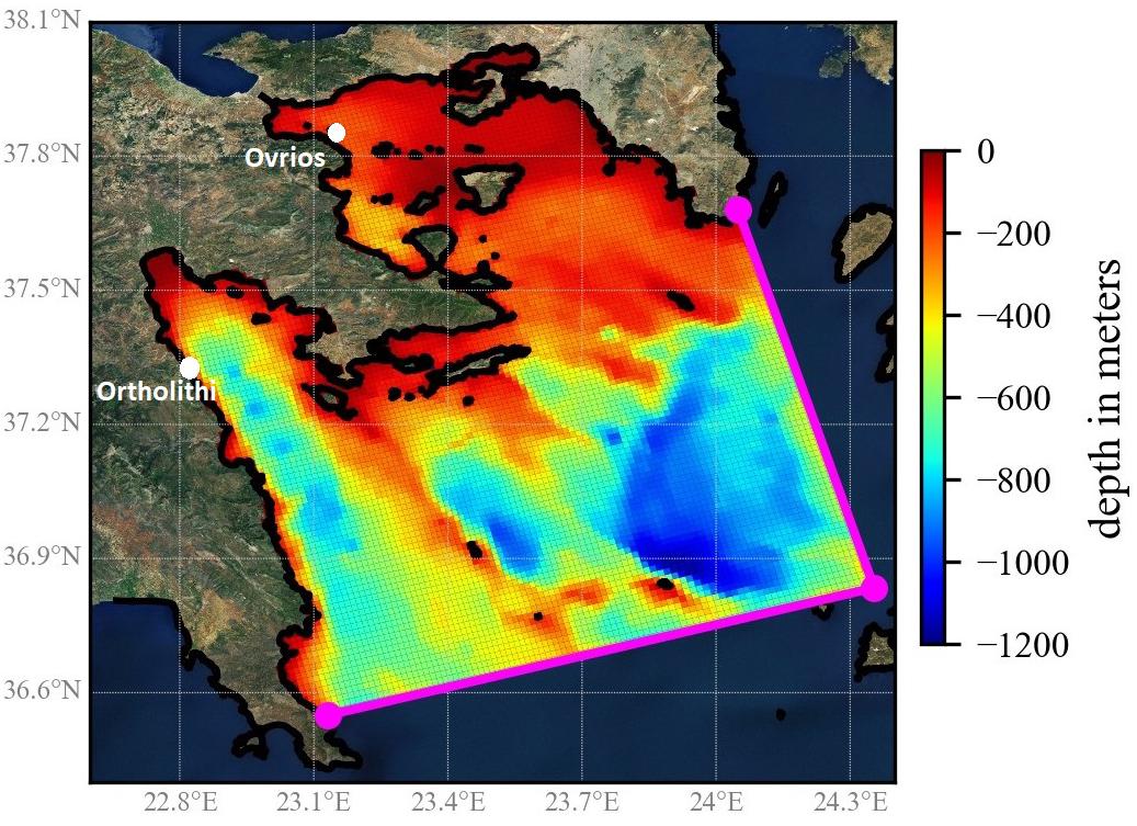
Figure 3. Seabed level in model domain. Two gulf areas have characteristic bathymetry, Saronic Gulf with shallow depths of ∼200–300 m and Argolic Gulf with deep sea trench of ∼ 400–800 m depth. Two Magenta lines indicating the boundary of the model domain.

Data

Bathymetry

In this model setup, the General Bathymetric Chart of the Oceans (GEBCO)² data was used for the bathymetry. The spatial resolution of the seabed level data used is 15 arc seconds (∼500 m) (Table 1). The seabed level values were embedded on the nodes of the numerical grid which is later used for various model computations (Figure 3).

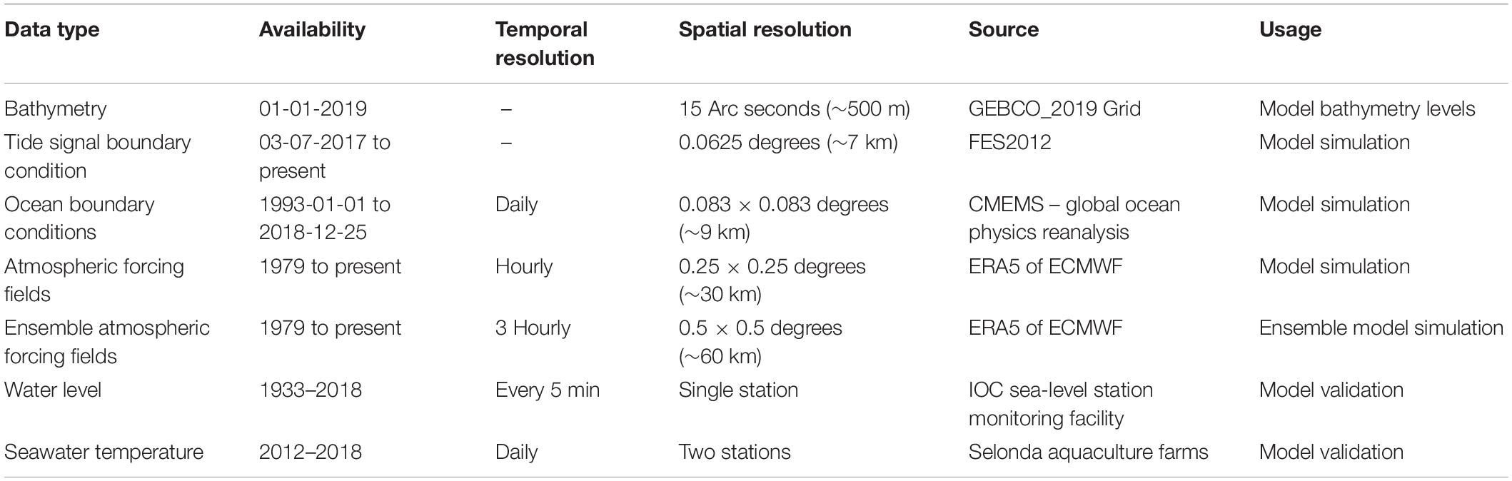
Table 1. List of data used in the study.

Boundary Condition

The study primarily uses data from Copernicus Marine Environment Monitoring Service (CMEMS) for the open boundaries. CMEMS is designed to provide crucial data related to marine environments mainly for European regional seas and the global oceans³. The European regional domains include the Arctic Sea, Baltic Sea, European North-West Shelf Sea, Iberia-Biscay-Ireland regional Sea, Mediterranean Sea, and the Black Sea. Their service is a product of integration between both satellite and in-situ data, followed by a state-of-the-art analysis using numerical models. CMEMS provides data for sea level, salinity, water temperature and biogeochemical variables such as oxygen, primary production, plankton, chlorophyll-a, among others. For the Mediterranean Sea, under CMEMS ocean products, biophysical parameters such as surface water levels, surface temperature, current velocities, reflectance, and chlorophyll-a concentrations, etc., are available⁴.

For the development of the hydrodynamic model boundary data such as astronomical tide signals, salinity, water temperature, steric water level, advection velocities were used (Figure 2). While tide signals are sourced from FES2012⁵, other boundary data are obtained from the global-reanalysis-phy-001-030-daily product of CMEMS⁴. This product has a spatial resolution of 0.083° × 0.083° (∼9 km) (Table 1). The vertical coverage ranges from 0.0 to 5500 m depth with 50 levels. These data are embedded at the two open sea boundaries of the model grid (Figure 3). We use global reanalysis data instead of the available Mediterranean solution as the present dynamical downscaling methodology is intended to be replicated for any geographical area, not only the Mediterranean Sea.

Atmospheric Forcing

The complete heat flux model was implemented in the model and this demands various atmospheric forcing data including solar radiation, wind, air temperature, dew point temperature, and cloud cover (Figure 2). Solar radiation is computed within Delft3D-flexible Mesh (DFM) depending on the time of the year and coordinate of the grid points (Deltares, 2019). Other information is obtained from ERA5 hourly data on single levels which is fifth-generation ECMWF atmospheric reanalysis of the global climate⁶. These data have a spatial resolution of 0.25° × 0.25° (∼30 km). Similarly, a 10-member ensemble with spatial resolution of 0.5° × 0.5° (∼60 km) available from ECMWF was used for probabilistic simulation and uncertainty analysis (Table 1). This 10-member ensemble covers all required atmospheric forcing data. It is based on physical considerations using an Ensemble of Data Assimilations (EDA) system, taking in to account the uncertainties in the ERA5 assimilation and modeling system⁷.

Validation Data

To validate the results of the hydrodynamic model, data from different sources were used (Figure 2). At first, the water level simulation was validated against the water level observations from Intergovernmental Oceanographic Commission (IOC) station at Peiraias (37°56′05.0″N 23°37′16.4″E), near Athens⁸ (Table 1). Simulation of the temperature was validated against the measured temperature at the two aquaculture sites - Ortholithi and Ovrios for the years 2016, 2017, and 2018. Farms have maintained long-term temperature measurement at both sites, measured at 8.00 h, 12.00 h, and 16.00 h and a daily average value is provided. These temperatures were measured at 4 m depth from the water surface. Various verification measures used in model validation are elaborated in the section “Verification measures.”

Methods

Numerical Modeling

The modeling tool employed in this research is the Delft3D-Flexible Mesh (DFM) modeling suite. Delft3D is a multi-dimensional (2D or 3D) hydrodynamic and transport simulation program which calculates non-steady flow and transport phenomena that result from tidal and meteorological forcing. It is widely used tool for hydrodynamic, sediment transport as well as water quality modeling. There are two computational schemes for heat transport in the model namely complete heat flux model and excess temperature model (Deltares, 2019). For the better representation of seawater related physical processes and increased accuracy the complete heat flux model was chosen. In the following equation, the heat balance at the sea surface is provided:

With R_S Solar radiation at the sea surface

L_e Latent heat flux (heat loss due to evaporation or gain by condensation)

IR Effective infrared back radiation

S Sensible heat flux

Each of the four components of equation (1) have a mathematical or empirical formulations which are detailed in Lane (1989). For the complete heat flux model to be implemented the model needs to be provided with atmospheric forcing data such as wind speed, solar radiation influx, air temperature, dew point temperature, and cloud cover. In DFM the solar radiation influx was calculated internally using model grid coordinate and time of the year. The rest of the atmospheric forcing data was provided externally. The details of the data used in the model development for setup, calibration and validation is provided in Table 1. The uniform horizontal grid resolution used in this study is ∼1 km × 1 km, whereas for vertical layering Z layer formulation (completely horizontal layers irrespective of water levels) was applied. Adaption of regular grid helps in achieving the orthogonality and smoothness criteria which otherwise is difficult to achieve for highly irregular coastline. The grid resolution of ∼1 km × 1 km is adapted considering few factors. Resolution of many input data are highly coarse. In such case finer grid resolution is not justified. Also, the SWT variability are not high in small spatial scales, unless there are small scale influx of heat. We use a Z layer thickness of 2 m for the top 40 m water depth. For the remaining depth, model chooses the Z layer depth with increasing thickness as depth increases. In the current model maximum of 47 Z layers are formed. The model simulation was performed for years 2016, 2017, and 2018. Deterministic and ensemble simulation experiments were setup with the above described boundaries and model forcings. The ensemble model outputs are further utilized in the analysis of uncertainties in temporal, spatial scales as well as along vertical gradients. We use several freely available python libraries for the data processing, analysis, plotting and mapping.

Verification Measures

Several verification measures are available to assess various statistical attributes associated with both deterministic and probabilistic simulations. In this paper, we used the measures proposed by Mészáros and El Serafy (2018), listed in Table 2. When the deterministic verification measures are to be used to assess ensemble simulations, one single plausible trace needs to be chosen from ensembles. In the study we chose the ensemble mean for the verification. The ensemble simulation results were also verified using probabilistic verification measures mentioned in Table 2. The probabilistic verification measures employed are Brier Score (Brier, 1950), Continuously Ranked Probability Score (Bröcker, 2012) and Receiver Operating Characteristics (ROC) curve (Hanley and McNeil, 1982).

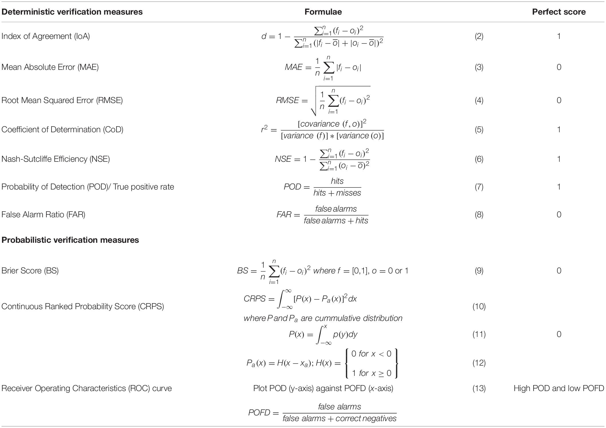
Table 2. Deterministic and probabilistic verification measures and formulae (f and o represent the model output and observed values respectively).

Uncertainty Analysis

The ensemble model outputs of SWTs need to be further processed using statistical methods to estimate the uncertainty. The most commonly used are ensemble spread and exceedance probabilities. For these statistical analyses to be performed, the distribution of the dataset must be known or assumed. Normal distribution is usually associated with water temperature and therefore was used in this study (Gneiting et al., 2005). Uncertainty was analyzed using ensemble spread which is the representation of the ensemble members in-terms of their mean (μ) and standard deviation (σ). In practice, ensemble spread is presented by using μ ± σ, μ ± 2σ, μ ± 3σ, etc.

Probability of exceedance (POE) takes probabilities of the occurrence of a defined event into account and is measured for a threshold value of interest. While analyzing the probabilities we focused on two thermal limits. Based on literature the upper and lower limits of SWT were considered as 26°C and 15°C (Mayer et al., 2008; Ibarz et al., 2010; Llorente and Luna, 2013; Balbuena-Pecino et al., 2019). Various studies specify varying thresholds for seabream. This is because some studies are laboratory based and some are field based studies. The process of arriving at POE involves defining Probability Density Function (PDF) f(x) and its Cumulative Distribution Function (CDF) F(x). From the CDF, for any given threshold value on x axis, corresponding y value gives probability of non-exceedance (p), from which one could estimate the probability of exceedance (1–p). These values of p and (1–p) are computed for both spatial maps and vertical temperature gradient maps.

For the uncertainty analysis in the spatial and vertical gradient, we focused on two seasons only. The months of February, March and April are considered the winter season in terms of the lower range of SWT, while the summer season can be attributed to the months of July, August and September. We are interested in the extreme SWT which occur in the months of March and August. These months are focus of the uncertainty analysis in the study. For simplification, we analyze the spatial and vertical scale uncertainty for the year 2017 only.

Results

Deterministic Model Results

Deterministic model results were obtained for seawater level (SWL) and seawater temperature (SWT). These results were further analyzed using verification measures listed in Table 2. The SWT model result was obtained at a temporal resolution of 1 h. In contrary the observation values of SWT were daily average measured three times between 8 AM and 4 PM. Therefore, the SWT model output was also taken as daily average between this time bracket of each day. The SWL simulation for the year 2018 was verified with deterministic verification measures. While overall range of SWL was 0.3 m to −0.3 m, the MAE and RMSE were considerably low at 0.057 and 0.070 m respectively. We accepted the moderate performance of the model for SWL as this was not having a major impact on the temperature model. The temperature model of DFM is a function of the atmospheric forcing such as solar radiation influx, wind speed, evaporation, etc.

Seawater Temperature (SWT) Simulation

Seawater temperature was simulated for 3 years from 2016 to 2018 for both stations - Ortholithi and Ovrios (Figure 7). In the figure, the observation value and simulated SWT (average value between 8 AM and 4 PM) are compared (Figure 7). The deterministic model performance was evaluated with verification measures listed in Table 2. The result of the verification measures is provided in Table 3. While the overall range of SWT is 14 – 28°C the errors are less than ∼1°C (Table 3). Other measures such as IoA, CoD and NSE yield values close to perfect score of 1. These values obtained from verification measures indicate that SWT results are satisfactory. There is a general agreement between the observed and simulated SWT, except for the year 2018 where the simulated values were slightly lower than observed values and the simulated yearly peak was reached few days earlier than observed values. This slight difference could be attributed to measurement errors or temporal changes in the model parameters which is not incorporated in the present study or lack of resolution in the input atmospheric forcing data. These data used in the model are coarser and therefore might not be accurate reflection of the actual atmospheric condition at site. The exact reason for the difference in 2018 needs further investigation, nevertheless, under current study it was not undertaken as this phase difference had little effect on seasonal analysis.

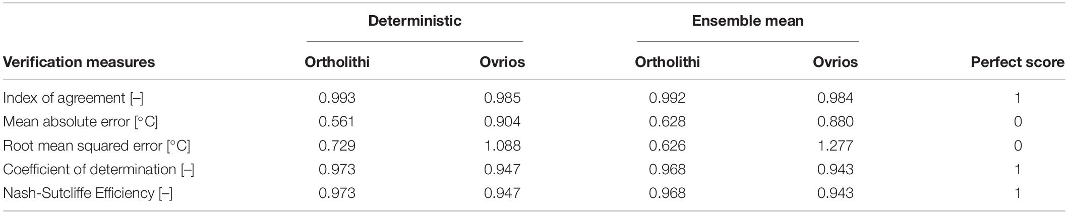
Table 3. Results of verification measures for deterministic SWT and ensemble mean SWT.

Ensemble Model Results

The ensemble SWT results for both observation sites were extracted in time series values. The performance of the ensemble model runs were evaluated using deterministic verification measures. For this purpose, a single trace of the ensemble runs needed to be selected for comparing with observed data. Instead of choosing one of the 10 members, we considered the mean of all 10 ensemble members. The evaluated verification measures are presented in Table 3. The error values calculated by MAE and RMSE are ∼0.6°C (Table 3). This is in comparison to the overall SWT range of 14 – 28°C was considered to be low. The error in SWT for both the stations shows similar trends, except for the initial 3–4 months when the model is in the initial spin-off period. The highest error is seen in the summer months of the year 2018 where model prediction is lower than the observation yielding negative error values. We also see a near perfect score values for IoA, CoD, and NSE, indicating at satisfactory model result (Table 3). Overall the performance of the model is better at Ortholithi compared to that of Ovrios. The reason could be that the available observed SWT values at Ovrios was coarser. These results are comparable to that of deterministic models (Table 3). We do not see any major improvement or decline between the two model results. Nevertheless, we can certainly quantify the uncertainties from ensemble results and provide probabilistic analysis of SWT both in spatial and vertical scales.

Ensemble model results were also spatially analyzed. The ensemble mean of SWT and ensemble spread in terms of 3σ maps were prepared for months of March and August for the year 2017 (Figure 4). It is apparent that the two gulf areas show different temperature behavior compared to the larger open sea (Figures 4A,C). This is most likely due to ease of heating or cooling of the water at shallow depths and lack of ocean circulations reaching the two gulf areas. During March (winter), Saronic Gulf show larger ensemble spread as compared to the Argolic Gulf. However, in August (summer), it is vice versa (Figures 4B,D). Such seasonal variation in ensemble spread could be a function of seasonal variability in the ensemble members of atmospheric forcings. This requires a further seasonal analysis of the atmospheric forcing data itself. However, the varying rates of mixing caused by varying levels of salinity or the currents can’t be ruled out. Vertical temperature gradient and vertical ensemble spread maps are shown in Figure 5. These are generated using model output at single computational cells for each month at the location of two farms. Winter months show clear mixing of water within 14°C – 16°C for entire depth with daily heating and cooling within the top 10 m (Figures 5A,C). In summer water column is thermally stratified. The top 20 – 30 m depth heats up to the temperature of 27°C in Ortholithi station (Figure 5E). For the same depth SWT is 25.5°C in Ovrios station (Figure 5G). From the ensemble spread maps, it is evident that errors are high in summer as compared to winter at both stations (Figure 5B,D,F,H). It can be associated with higher rate of turbulence in the season or other ocean variables such as salinity, currents causing the varying rates of mixing. The exact cause for temporal, spatial and vertical scale variations in the ensemble spread need further detailed study with other ocean variables such as – salinity, currents and turbulences.

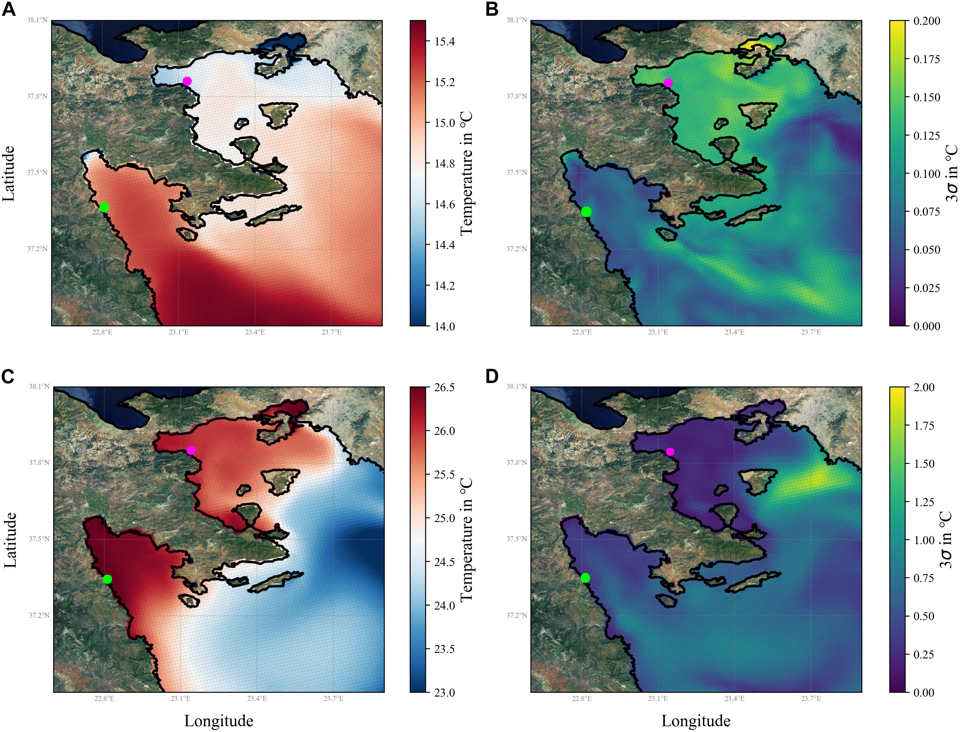
Figure 4. Ensemble mean and ensemble spread of SWT with two aquaculture farms marked – Ortholithi (Green dot) and Ovrios (Magenta dot) (A) monthly mean March 2017, (B) 3 standard deviations (σ) March 2017, (C) monthly mean August 2017, and (D) 3σ August 2017.

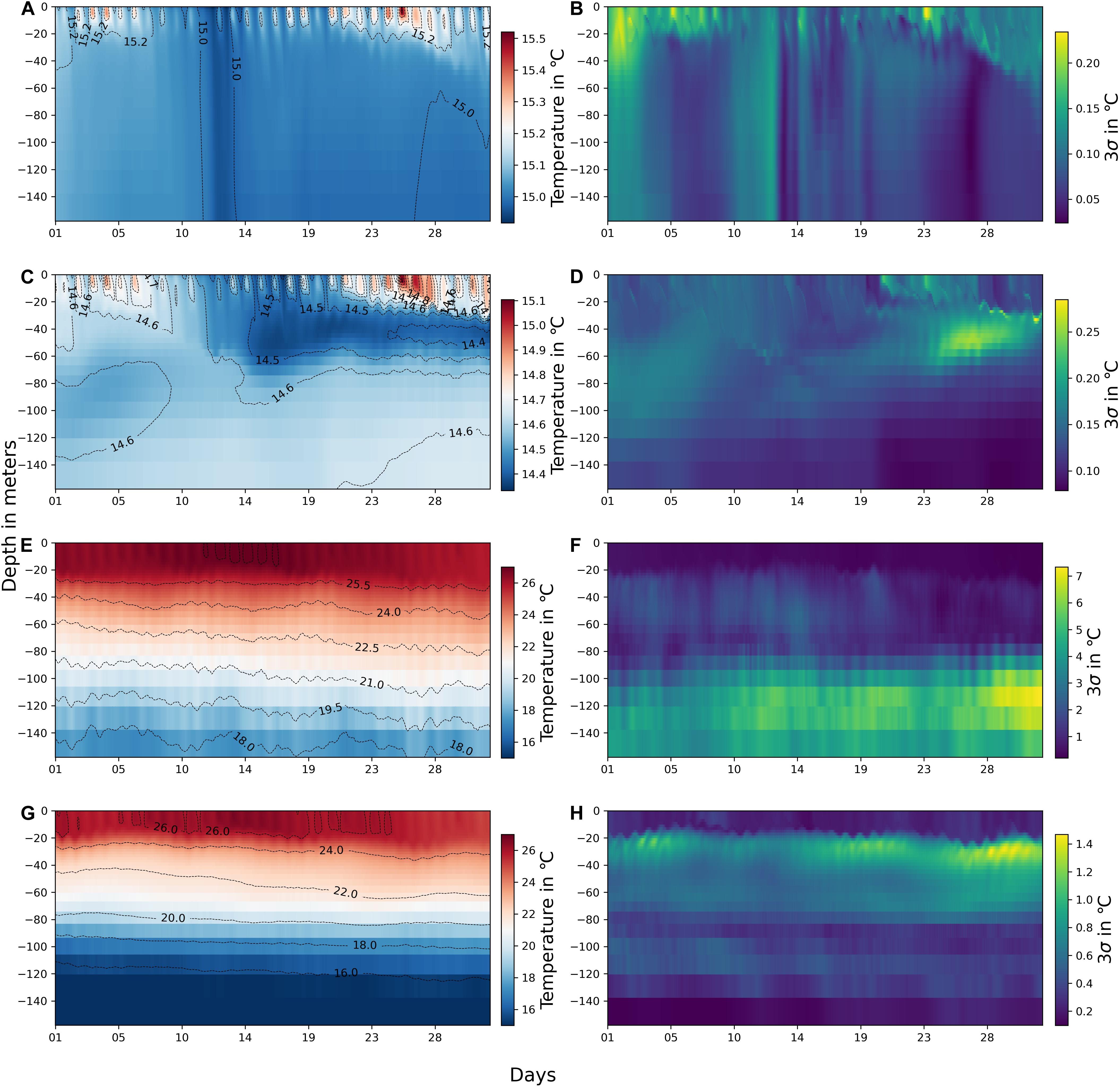
Figure 5. Ensemble mean and ensemble spread of vertical SWT (A) Mean – Ortholithi March 2017, (B) 3 standard deviations (σ) – Ortholithi March 2017, (C) Mean – Ovrios March 2017, (D) 3σ – Ovrios March 2017, (E) Mean – Ortholithi August 2017, (F) 3σ – Ortholithi August 2017, (G) Mean – Ovrios August 2017, and (H) 3σ – Ovrios August 2017.

Probabilistic Verification Measures

We performed previously explained probabilistic verification measures to assess the performance of the ensemble simulations. For this purpose, we used Brier Score (BS), Continuous Ranked Probability Score (CRPS) and Receiver Operating Characteristics (ROC) curve. Two stations Ortholithi and Ovrios were individually assessed for the probabilistic verification measures for all the 3 years of simulation – 2016–2018. For both BS and CRPS we used two different threshold temperatures to assess the values. The lower temperature threshold of 15°C and an upper threshold of 26°C was used. In case of the lower threshold, the criteria of assessment were to verify if the model simulation predicted the temperatures ≤ 15°C when observed temperature was ≤15°C. In case of the upper threshold, the criteria of assessment were to verify if the model simulation predicted the temperatures ≥ 26°C when observed temperatures were ≥26°C.

Based on both BS and CRPS results the ensemble model performance was better in predicting the upper limit temperature than lower limit temperature. In general, the performance of the model was better at the station Ortholithi both in the prediction of lower and upper limit temperatures (Table 4). Large difference in CRPS value was seen in Ovrios for 15°C threshold. Ensemble model performed better in this case. On the other hand, slight decline in ensemble performance was noted in Ovrios for 26°C threshold. Ortholithi showed slight improvement in ensemble performance for 26°C threshold. At the same time, no significant difference for 15°C threshold was noticed.

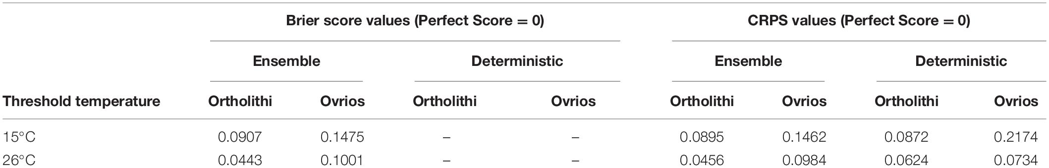
Table 4. Brier score and Continuous Ranked Probability Score (CRPS) values computed for two stations.

Receiver operating characteristics curve plots the true positive rate against the false-negative rate, which are essentially comparing the model result and observed data. A perfect prediction is one that shows a high true positive rate and a low false negative rate. Therefore, the perfect prediction results in the ROC curve on the upper left side of the diagonal line. Among all the plots, the one for non-exceedance of 15°C at Ortholithi performed poorly (Figure 6A). This ROC curve was over the diagonal line indicating poor ability to distinguish between events and non-events. However, at the same time, Ortholithi station showed higher performance in predicting exceedance of 26°C (Figure 6C). Both the models showed good ability to distinguish between events and non-events for the Ovrios station for both thresholds (Figures 6B,D). Except for the 26°C threshold at Ovrios, all other cases showed improved performance of the ensemble simulation compared to deterministic models. This result was consistent with the CRPS scores, where the deterministic model outperformed the ensemble model for the 26°C threshold at Ovrios station.

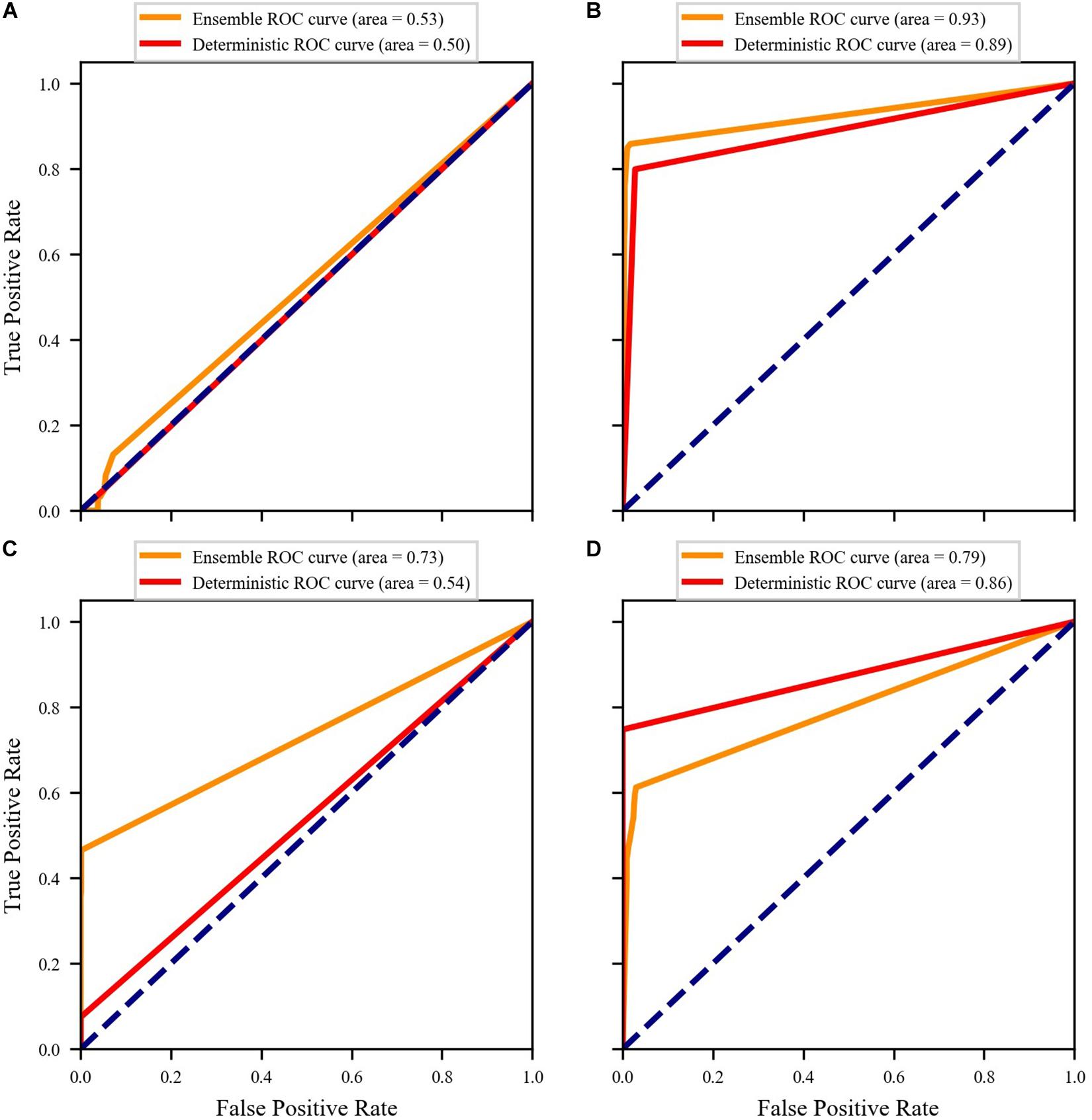
Figure 6. Receiver operating characteristics (ROC) curves for two stations (A) 15°C threshold – Ortholithi, (B) 15°C threshold – Ovrios, (C) 26°C threshold – Ortholithi, (D) 26°C threshold – Ovrios. The dashed line represent the 1:1 line.

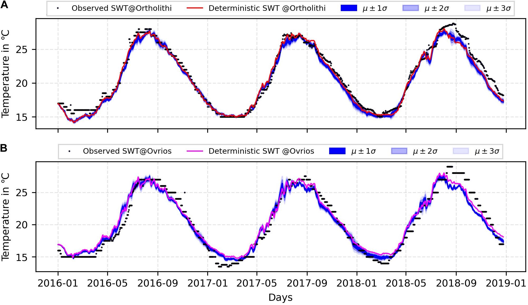
Figure 7. Ensemble spread of SWT simulation for (A) Ortholithi (B) Ovrios together with observations and deterministic simulation.

Uncertainty Analysis

Ensemble spread plots were prepared by plotting mean (μ) ± standard deviations (σ) for each time step. In Figure 7, μ ± σ, μ ± 2 σ, and μ ± 3 σ are shown. From these plots, it may be observed that the uncertainty in the SWT shows a seasonal trend. Uncertainty was comparatively high during the summer months of July, August, and September. Overall the ensemble spread was narrow within ∼1°C uncertainty range. This range of spread was low indicating that atmospheric ensembles had very limited influences on the SWT simulation.

Probability of exceedance and non-exceedance were evaluated spatially over the entire model domain for the representative months, March and August according to the method specified in section “Uncertainty analysis.” When dealing with a lower thermal limit of 15°C, the probability of non-exceedance was applied. When dealing with the upper thermal limits of 26°C, the probability of exceedance was applied. These maps show the variability of the probabilities in the spatial scale. From maps in Figure 8, we note that, the probability of non-exceedance of the lower threshold temperature is greater in the Saronic Gulf than in the Argolic Gulf (Figure 8A). Both the gulf areas show a high probability of exceeding the upper threshold temperature (Figure 8B).

Figure 8. Spatial maps of probability of (A) non-exceedance of 15°C – March 2017 (B) exceedance of 26°C – August 2017.

Probability of exceedance and non-exceedance were evaluated over water depths at two stations to understand the vertical behavior of the probabilities. At Ortholithi, probability of non-exceedance of 15°C in the month of March was high only for 10 days in the month and occurred in daily cycles (Figure 9A). There was a high probability of exceeding the 26°C threshold in the upper 20 m depth in the month of August (Figure 9B). The stratification that is observed in the summer month is replaced by mixed water resulting in a fluctuating probability of non-exceedance of lower limit temperature. At Ovrios, the probability of non-exceedance of the 15°C threshold was uninterrupted for whole month of March (Figure 9C). The probability of exceeding 26°C is high for about 10 – 20 m depth which is regularly interrupted by the lower probability of exceedance (Figure 9D).

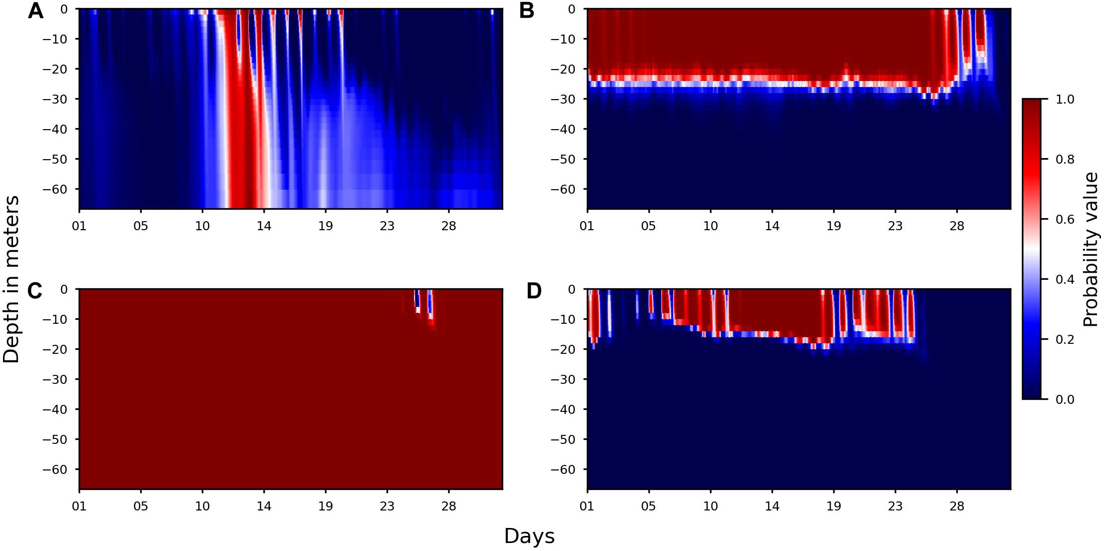
Figure 9. Vertical plots of probability of (A) non-exceedance of 15°C at Ortholithi – March 2017, (B) exceedance of 26°C at Ortholithi – August 2017, (C) non-exceedance of 15°C at Ovrios – March 2017, and (D) exceedance of 26°C at Ovrios – August 2017.

It is important to note that these probabilities are not compared to the observed values. We already noted that many of the observed values fall outside the ensemble spread (Figure 7). The time series comparison are only made at two observation locations at surface and therefore have limitation in representing the whole model domain and the model depth. The spatial and vertical scale probabilities reveal the regions and depths that are susceptible to be in thermal limits. Therefore these information are still relevant in operational planning in aquaculture farms.

Discussion

In the study, we demonstrated an ensemble modeling of SWT and in principle, this study may be replicated to any geographical location. The data sets that are used are freely available making model development possible. The combination of DFM modeling tool along with CMEMS boundary conditions, ERA5 atmospheric forcing fields and GEBCO bathymetry was adopted in this study. The use of coarser global CMEMS data yields satisfactory results. This also widens scopes for using higher resolution regional data sets of CMEMS in further studies. In the study we utilized the 10 member atmospheric forcing fields of ERA5 with each member consisting of four variables – 2 m air temperature, 2 m dew point temperature, 10 m wind speed and cloud cover. This yielded a narrow ensemble spread with some of the observation data outside the ensemble spread.

We performed the deterministic verification measure such IoA, MAE, RMSE, CoD and NSE for the two stations. From the results, we did not see a significant improvement in the ensemble predictions as compared to the deterministic predictions. However, the probabilistic verifications of CRPS and ROC curves show that ensemble model provides slightly better threshold predictions of thermal limits than a deterministic prediction. This is true for all cases except for the 26°C threshold at Ovrios.

Atmospheric forcing fields did not result in larger ensemble spread. Some of the extreme SWT values are outside the bounds of ensemble spread. Also the trend in the observed SWT in the year 2018 is not reflected in both the model results. The study attempted to quantify the uncertainty from single source, i.e., atmospheric forcing. However, there is need to include other sources of uncertainties such as model parameter uncertainty. From the investigation into the temperature model of DFM, it is noted that the parameters such as secchi depth (SD) – a measurement of water transparency, eddy diffusivity and eddy viscosity terms could be potential candidates for further investigation into model parameter uncertainty. The absorption of heat in the water column is an exponential function of the distance from the water surface, which is largely controlled by the parameter SD. SD is relatively simpler technique of measuring the transparency of water column. A circular disk attached to rope is dropped in water column and depth at which it is no longer visible to naked eye is measured as SD. Evidently, higher the value of SD, higher is the transparency of water. This means, more solar radiation can reach the deeper waters. However, true value of the parameter is not available for part of the Aegean Sea. In this study, we used 10 m secchi depth value. Further uncertainty arising from the SD needs to be quantified with varying SD values. Similarly, parameters such as eddy diffusivity and eddy viscosity play crucial role in the turbulence model used in the numerical setup. In the current study we employed k-ε turbulence model, which takes both turbulent kinetic energy (k) and turbulent dissipation rate (ε) into account. These parameters determines the mixing of water under turbulent condition and therefore control the temperature fluctuations both in horizontal and vertical scales. Further uncertainty quantification need to be conducted for these parameters. Most reliable course of action for the future studies is to quantify the uncertainties arising from the model parameters.

We noted that there were regions within the model domain which showed consistent probabilities for upper and lower thermal thresholds. Furthermore, we observed that both the gulf areas showed a high probability of exceeding the upper limit, while the probability of non-exceedance of the lower limit was greater in the Saronic Gulf than in the Argolic Gulf. Ortholithi station did not exhibit high non-exceedance probability for 15°C, contrary to Ovrios station which showed high non-exceedance probability for 15°C, with daily interruptions of low probability. Therefore, Ovrios station is more susceptible to the lower thermal limits than Ortholithi station during winter. Analysis of vertical gradient of the temperature and its probabilities reveal that in summer seasons there is a clear stratification of water with high probabilities of exceeding upper thermal limit at top ∼20 m depth. Therefore, the existing cage depth of 10 m at two stations are not sufficiently deep to offer comfortable SWT for fishes in summer. This is also useful while developing new cages in the region. The thermal stratification is replaced by mixed water in the winter season. This resulted in entire column of water showing homogenized water temperature. Such a scenario gives no scope for changes in depth of the cage. Therefore, different operational change needs to be followed, for example change in the diet plan or feeding rate to suit SWT. These information is particularly important for establishment of new farms in the region. Farmers could make use of the established regional behavior to select areas of suitable SWT throughout the year. The ability to distinguish differences in SWT behavior in two Gulf areas is a useful mechanism in earmarking areas of high potential for aquaculture farms. Such information is useful for coastal development authorities in spatial planning. However, in this study we used SWT information alone, more comprehensive planning could be made by including other ocean variables such as salinity, currents, dissolved oxygen, and nutrient concentrations.

In the current study we used a uniform ∼1 km × 1 km spatial resolution. With varying resolution of grid cells, where finer cells are formed near the coasts, it is possible to investigate the small scale SWT variations, caused by small scale turbulences. However, the scope for a finer resolution model is limited by the resolution of the input data, i.e., atmospheric forcings and bathymetry. Unless these input data are available at finer resolution, more resolved model grid would not improve the model performance. Other ocean variables, i.e., salinity, currents, dissolved oxygen, and nutrient concentrations are considered to vary significantly within a small spatial scale depending on sources and sinks. When these variables are to be considered, finer grid needs to be employed. It should be noted that the study deals with a coastal system, however, aquaculture sites are established in coastal lagoons, estuaries and river delta around the world for varying reasons. In such a scenario, input of freshwater, sediment and high nutrient concentration is expected from land. As we move from coastal systems to fluvial systems, the spatial scale reduces. This demands finely refined model discretization in order to capture the small scale fluctuations in the fluvial systems. Moreover, boundary condition data from the fluvial systems needs to be provided for better representation of the natural phenomenon.

The simulation was performed for years from 2016 to 2018. In this period three summers and two winter periods were studied for uncertainty quantification. However, to understand the long-term fluctuations in SWT, decadal model simulations might be required. The validation of the model performance was done at two stations for which data was secured from the aquaculture farms. We successfully validate the model in spatial and temporal scale. The lack of any monitoring stations with access to vertical SWT data hinders vertical scale validation of the model simulation. Remote sensing data both in spatial and vertical scale is another possibility for model validation. This would enable validation of the model in all three dimensions. Therefore, validation of model with remote sensing data stands as major work for future studies.

Conclusion

The aquaculture sector needs SWT information for crucial operational decisions at the farms. Present ad hoc measurement of SWT could only provide information for the present state of the sea and could not give information on the harmful events in future. We build on the existing knowledge on a specific fish species and translate that knowledge for aiding decision making using a numerical modeling tool. This study used numerical modeling along with ensemble simulation of SWT to provide uncertainty assessment to benefit the operations of the aquaculture farms, which is presently not a common practice. We successfully demonstrated modeling tool which simulates the SWT with satisfactory results and accomplished to assess SWT in temporal, seasonal as well as vertical scales from an aquaculture perspective. Study demonstrated that information of vertical behavior of the SWT is key for the aquaculture farms’ operations as it has shown different behavior in different regions and seasons. These information are not possible to generate from in-situ measurements alone. Study extends the data available from larger open seas to the remote coastal areas where data is required for the businesses. It is evident that more uncertainty sources need to be further assessed in order to quantify the total uncertainty in the SWT predictions. Authors recognize that even though predicted SWT is useful in making decisions, further value to the study could be added by combining SWT prediction with fish physiology. Such a model links the water quality variables such as SWT, salinity, nutrient concentrations, etc., to the fish growth and subsequently to the economy of the aquaculture farm.

Data Availability Statement

Publicly available datasets were analyzed in this study. This data can be found here: https://download.gebco.net/, https://www.aviso.altimetry.fr/en/data/products/sea-surface-height-products/global.html, https://resources.marine.copernicus.eu/?option=com_csw&view=details&product_id=GLOBAL_REANALYSIS_PHY_001_030, and http://www.ioc-sealevelmonitoring.org/station.php?code=pei.

Author Contributions

NS developed the research topic under the guidance of BB and GE. NS wrote the initial manuscript which was reviewed and edited by BB, GE, and LM. LM and AS contributed to the data processing and analysis. All the authors contributed to the article and approved the submitted version.

Funding

This project was co-funded by the European Union’s Horizon 2020 Research and Innovation Programme under Grant Agreement No. 821934.

Conflict of Interest

The authors declare that the research was conducted in the absence of any commercial or financial relationships that could be construed as a potential conflict of interest.

Acknowledgments

We would like to acknowledge ECMWF, CMEMS, and GEBCO for allowing open access to the data. We thank SELONDA for providing crucial data related to aquaculture farms. Special thanks to colleagues at Deltares for support at various levels of the study.

Footnotes

1. ^ https://ec.europa.eu/fisheries/sites/fisheries/files/docs/body/op-greece-fact-sheet_en.pdf
2. ^ https://download.gebco.net/
3. ^ https://www.copernicus.eu/sites/default/files/documents/Copernicus_MarineMonitoring_Feb2017.pdf
4. ^ https://resources.marine.copernicus.eu/?option=com_csw&view=details&product_id=GLOBAL_REANALYSIS_PHY_001_030
5. ^ https://www.aviso.altimetry.fr/en/data/products/sea-surface-height-products/global.html
6. ^ https://cds.climate.copernicus.eu/cdsapp#!/dataset/reanalysis-era5-single-levels?tab=overview
7. ^ https://confluence.ecmwf.int/display/CKB/ERA5%3A+uncertainty+estimation#app-switcher
8. ^ http://www.ioc-sealevelmonitoring.org/station.php?code=peir

References

Balbuena-Pecino, S., Riera-Heredia, N., Vélez, E. J., Gutiérrez, J., Navarro, I., Riera-Codina, M., et al. (2019). Temperature affects musculoskeletal development and muscle lipid metabolism of gilthead sea bream (Sparus aurata). Front. Endocrinol. 10:173. doi: 10.3389/fendo.2019.00173
Bell, J. D., Ganachaud, A., Gehrke, P. C., Griffiths, S. P., Hobday, A. J., Hoegh-Guldberg, O., et al. (2013). Mixed responses of tropical Pacific fisheries and aquaculture to climate change. Nat. Clim. Change 3, 591–599. doi: 10.1038/nclimate1838
Berlinsky, D., Taylor, J., Howell, R., Bradley, T., and Smith, T. (2007). The effects of temperature and salinity on early life stages of black sea bass Centropristis striata. J. World Aquacul. Soc. 35, 335–344. doi: 10.1111/j.1749-7345.2004.tb00097.x
Besson, M., Vandeputte, M., van Arendonk, J. A. M., Aubin, J., de Boer, I. J. M., Quillet, E., et al. (2016). Influence of water temperature on the economic value of growth rate in fish farming: the case of sea bass (Dicentrarchus labrax) cage farming in the Mediterranean. Aquaculture 462, 47–55. doi: 10.1016/j.aquaculture.2016.04.030
Brier, G. W. (1950). Verification of forecasts expressed in terms of probability. Mon. Weather Rev. 78, 1–3. doi: 10.1175/1520-04931950078<0001:Vofeit<2.0.Co;2
Bröcker, J. (2012). Evaluating raw ensembles with the continuous ranked probability score. Q. J. R. Meteorol. Soc. 138, 1611–1617. doi: 10.1002/qj.1891
Buizza, R. (2018). Introduction to the special issue on “25 years of ensemble forecasting. Q. J. R. Meteorol. Soc. 145, 1–11. doi: 10.1002/qj.3370
Callaway, R., Shinn, A., Grenfell, S., Bron, J., Burnell, G., Cottier-Cook, E., et al. (2012). Review of climate change impacts on marine aquaculture in the UK and Ireland. Aquat. Conserv. Mar. Freshw. Ecosyst. 22, 389–421. doi: 10.1002/Aqc.2247
Chaudhuri, A. H., Ponte, R. M., and Forget, G. (2016). Impact of uncertainties in atmospheric boundary conditions on ocean model solutions. Ocean Modelling 100, 96–108. doi: 10.1016/j.ocemod.2016.02.003
FAO (2011). National Aquaculture Legislation Overview - Greece. Available: http://www.fao.org/fishery/legalframework/nalo_greece/en (accessed 12 Febraury 2020).
FAO (2020). The State of World Fisheries and Aquaculture 2020. Rome: Food and Agriculture Organisation.
Gneiting, T., Raftery, A., Westveld, A., and Goldman, A. (2005). Calibrated probabilistic forecasting using ensemble model output statistics and minimum CRPS estimation. Mon. Weather Rev. 133, 1098–1118. doi: 10.1175/MWR2904.1
Hanley, J. A., and McNeil, B. J. (1982). The meaning and use of the area under a receiver operating characteristic (ROC) curve. Radiology 143, 29–36. doi: 10.1148/radiology.143.1.7063747
Hobday, A. J., Spillman, C. M., Paige Eveson, J., and Hartog, J. R. (2016). Seasonal forecasting for decision support in marine fisheries and aquaculture. Fish. Oceanogr. 25(Suppl. 1), 45–56. doi: 10.1111/fog.12083
Hurst, T. (2007). Causes and consequences of winter mortality in fishes. J. Fish Biol. 71, 315–345. doi: 10.1111/j.1095-8649.2007.01596.x
Ibarz, A., Padrós, F., Gallardo, M., Fernández-Borràs, J., Blasco, J., and Tort, L. (2010). Low-temperature challenges to gilthead sea bream culture: review of cold-induced alterations and ‘Winter Syndrome’ Rev. Fish Biol. Fish. 20, 539–556. doi: 10.1007/s11160-010-9159-5
Kassis, D., Krasakopoulou, E., Gerasimos, K., Petihakis, G., and Triantafyllou, G. (2016). Hydrodynamic features of the South Aegean Sea as derived from Argo T/S and dissolved oxygen profiles in the area. Ocean Dyn. 65, 1449–1466. doi: 10.1007/s10236-016-0987-2
Lima, L., Pezzi, L., Penny, S., and Tanajura, C. (2019). An investigation of ocean model uncertainties through ensemble forecast experiments in the southwest Atlantic Ocean. J. Geophys. Res. 124, 432–452. doi: 10.1029/2018JC013919
Llorente, I., and Luna, L. (2013). The competitive advantages arising from different environmental conditions in seabream. Sparus aurata, Production in the Mediterranean Sea. J. World Aquacul. Soc. 44, 611–627. doi: 10.1111/jwas.12069
Lorentzen, T. (2008). Modeling climate change and the effect on the Norwegian salmon farming industry. Nat. Resour. Modeling 21, 416–435. doi: 10.1111/j.1939-7445.2008.00018.x
Martin, Q., Julia, H., Katrin, K., Linda, K., and Karoline, S. (2016). Fishing for Proteins. Hamburg: WWF Germany.
Masroor, W., Farcy, E., Gros, R., and Lorin-Nebel, C. (2018). Effect of combined stress (salinity and temperature) in European sea bass Dicentrarchus labrax osmoregulatory processes. Comp. Biochem. Physiol. Part A Mol. Integr. Physiol. 215, 45–54. doi: 10.1016/j.cbpa.2017.10.019
Mayer, P., Estruch, V., Blasco, J., and Jover, M. (2008). Predicting the growth of gilthead sea bream (Sparus aurata L.) farmed in marine cages under real production conditions using temperature- and time-dependent models. Aquacul. Res. 39, 1046–1052. doi: 10.1111/j.1365-2109.2008.01963.x
Merino, G., Barange, M., Blanchard, J., Harle, J., Holmes, R., Allen, I., et al. (2012). Can marine fisheries and aquaculture meet fish demand from a growing human population in a changing climate? Glob. Environ. Change 22, 795–806. doi: 10.1016/j.gloenvcha.2012.03.003
Mészáros, L., and El Serafy, G. (2018). Setting up a water quality ensemble forecast for coastal ecosystems: a case study of the southern North Sea. J. Hydroinform. 20, 846–863. doi: 10.2166/hydro.2018.027
Olson, D., Kourafalou, V., Johns, W., Samuels, G., and Veneziani, M. (2007). Aegean surface circulation from a satellite-tracked drifter array. J. Phys. Oceanogr. 37, 1898–1917. doi: 10.1175/JPO3028.1
Person-Le Ruyet, J., Mahé, K., Le Bayon, N., and Le Delliou, H. (2004). Effects of temperature on growth and metabolism in a Mediterranean population of European sea bass. Dicentrarchus labrax. Aquaculture 237, 269–280. doi: 10.1016/j.aquaculture.2004.04.021
Pesce, M., Critto, A., Torresan, S., Giubilato, E., Pizzol, L., and Marcomini, A. (2019). Assessing uncertainty of hydrological and ecological parameters originating from the application of an ensemble of ten global-regional climate model projections in a coastal ecosystem of the lagoon of Venice. Italy. Ecol. Eng. 133, 121–136. doi: 10.1016/j.ecoleng.2019.04.011
Richardson, D. S. (2000). Skill and relative economic value of the ECMWF ensemble prediction system. Q. J. R. Meteorol. Soc. 126, 649–667. doi: 10.1002/qj.49712656313
Keywords: aquaculture, dynamic downscaling, ensemble simulation, seabream, seawater temperature, uncertainty analysis
Citation: Shettigar NA, Bhattacharya B, Mészáros L, Spinosa A and El Serafy G (2020) 3D Ensemble Simulation of Seawater Temperature – An Application for Aquaculture Operations. Front. Mar. Sci. 7:592147. doi: 10.3389/fmars.2020.592147
Received: 06 August 2020; Accepted: 03 November 2020;
Published: 24 November 2020.
Edited by:
Agustin Sanchez-Arcilla, Universitat Politecnica de Catalunya, SpainReviewed by:
Rafael O. Tinoco, University of Illinois at Urbana–Champaign, United StatesMeadhbh Moriarty, Ulster University, United Kingdom
Copyright © 2020 Shettigar, Bhattacharya, Mészáros, Spinosa and El Serafy. This is an open-access article distributed under the terms of the Creative Commons Attribution License (CC BY). The use, distribution or reproduction in other forums is permitted, provided the original author(s) and the copyright owner(s) are credited and that the original publication in this journal is cited, in accordance with accepted academic practice. No use, distribution or reproduction is permitted which does not comply with these terms.
*Correspondence: Ghada El Serafy, Ghada.ElSerafy@deltares.nl