A Multiparametric Approach to Study the Preparation Phase of the 2019 M7.1 Ridgecrest (California, United States) Earthquake

Introduction

The 2019 Ridgecrest seismic sequence started on July 4, 2019: many small magnitude events (Ml ∼ 0) preceded by 2 h the major earthquake with a 6.4 magnitude (Ross et al., 2019), occurred at 17:33 UTC on 4 July and now considered as the largest foreshock. The sequence of foreshocks continued with numerous events with magnitude from intermediate to large (e.g., an M5.4 about 16 h, and an M5.0 almost 3 min before the mainshock) culminating with the M7.1, which struck on 6 July at 03:19 UTC. This earthquake was the most powerful event occurring in California in the last 20 years (after the M7.1 1999 Hector Mine earthquake, e.g., Rymer et al., 2002). These major shocks occurred north and northeast of the town of Ridgecrest, California (about 200 km north-northeast of Los Angeles). After 21 days, they were followed by more than 111,000 aftershocks (M > 0.5, Ross et al., 2019), mainly within the area of the Naval Air Weapons Station China Lake (California).

Recent works on the Ridgecrest seismic sequence revealed much of the complexity of the seismic source of the major ruptures and relative mechanisms (e.g., Barnhart et al., 2019; Ross et al., 2019; Chen et al., 2020), but nothing was investigated about the preparation phase of the seismic sequence and its possible coupling with the above geolayers, such as the atmosphere and ionosphere. This article intends to fill the gap.

We know how much difficult the study of what happens before a large earthquake is and how controversial the concept of preparation phase of an earthquake is within the scientific community. Nevertheless, it is rather difficult to think that a so large energetic phenomenon such as a strong earthquake cannot provide any sign of its preparation (e.g., Sobolev et al., 2002; Bulut 2015). With this work, we want to give a fundamental contribution to the study of the preparation phase of earthquakes, considering the case study of the 2019 Ridgecrest seismic sequence.

The idea of an interconnected planet where all its parts interact each other is known as geosystemics (De Santis, 2009; De Santis, 2014) and it is a very interesting concept to apply to the study of earthquakes (De Santis et al., 2019a). This idea suggests that the best way to study Earth’s physical phenomena is a multiparametric analysis. This means that, in order to understand how some processes work, we need to analyze different parameters from the area of interest, originating from different sources. In the particular case of earthquakes, the lithosphere-atmosphere-ionosphere coupling (LAIC) proposes a relation between events occurred in lithosphere, atmosphere, and ionosphere that could precede the occurrence of large earthquakes. Therefore, the study of the preparation phase of large earthquakes, as this one in California, can be especially useful to identify possible precursors. There exist different models to explain how these three layers could be linked to each other. A model predicts at fault level the existence of p-holes (positive holes) that, once released at the surface, are able to ionize the atmosphere (Freund, 2011; Freund, 2013) and finally reach the ionosphere. Another model is based on a gas or fluid (such as radon) that can be released by the lithosphere during the preparation phase of earthquake (Pulinets and Ouzounov, 2011; Hayakawa et al., 2018). Both models foresee the creation of a chain of processes that connects the lithosphere to the atmosphere and then to the ionosphere.

In this work, we analyze data from the lithosphere (earthquakes), atmosphere (temperature, water vapor, aerosol, and methane), and ionosphere (e.g., electron density, magnetic field, and other ionospheric parameters) in order to possibly identify the chain of processes preceding the seismic sequence of concern. Limited ground-based observations have been also incorporated. Such an approach demonstrated its powerful capability also in some previous case studies (e.g., Akhoondzadeh et al., 2018; Akhoondzadeh et al., 2019; Marchetti et al., 2019a; Marchetti et al., 2019b; Marchetti et al., 2020), when the view of the earthquake is wider (geosystemic view) and includes all the geolayers involved in the processes (De Santis et al., 2019a; De Santis et al., 2019b).

Being a multiparametric approach, the statistics we applied in this article depends on the parameter and its historical availability (e.g., while atmospheric data have a long history of about 40 years, the satellite data are rather short, about 6 years, so we had to resort to another approach). For the single parameters and their methodology of analysis, we already conducted some statistical validations in our previous works, i.e., skin temperature and total column water vapor analyzed by Climatological Analysis for seismic PRecursor Identification (CAPRI) algorithm have been statistically demonstrated to be successfully related as EQ-precursors in Central Italy in the last 25 years (with 73–74% of overall accuracy; Piscini et al., 2017). The accelerated moment release (AMR) seismic methodology has been successfully validated on 14 medium-large earthquakes (M6.1–M8.3), providing statistical evidence on this set of events that the technique is able to detect a seismic acceleration (Cianchini et al., 2020).

Data Analyses

A seismic characterization of the sequence was conducted by inspecting data collected by the Southern California Earthquake Data Center (SCEDC): we downloaded its catalog from January 1, 2000, to November 13, 2019 (last visit November 14, 2019).

Then, we restricted the events in time (t), depth (z), and magnitude (M) by setting the threshold values to 2000.0 ≤ t < 2019.51 (this later being the mainshock origin time in decimal year), z ≤ 50 km and M ≥ 2, respectively: from now on, this is the complete catalog considered for our analyses. Figure 1 represents the seismicity of South California as emerged by the imposed limits. The epicenter and the focal mechanism of the M7.1 mainshock are shown. The thick white line shows approximately (more detailed in Figure 2 by Ross et al., 2019) the projection on the surface of the rupture plane as is depicted by the sequence of the aftershocks. In evidence, a green star shows the strongest foreshock (M6.4), which preceded by almost 34 h the main event, indicated by a red star.

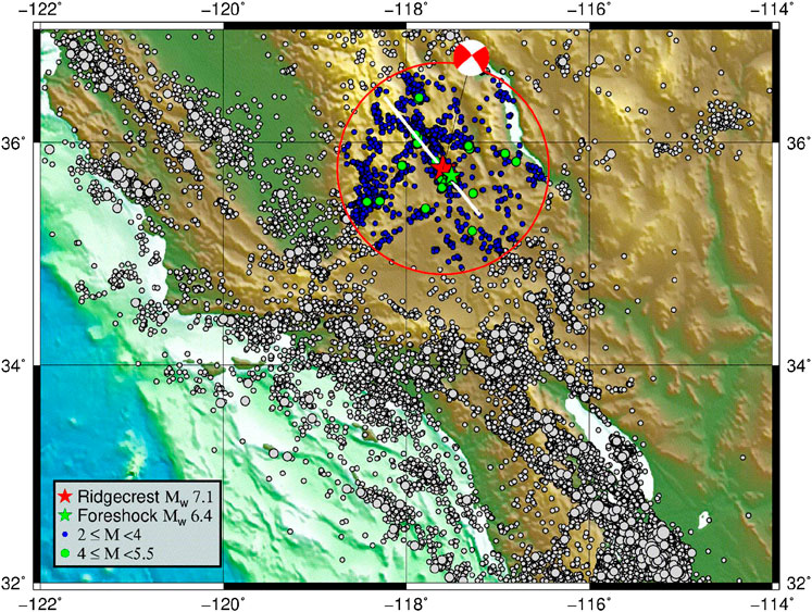
FIGURE 1. Spatial distribution of earthquake epicenters from 2000 to 2019.5. The thick white line at the central top represents approximately the projection on the surface of the rupture plane, which has been depicted by the aftershocks of the Ridgecrest main event (realized by the GMT Tool). The red circle has a radius of 100 km and is explained in the text. The earthquakes outside the circular areas are presented without colors, but the size corresponds to the range of magnitudes.

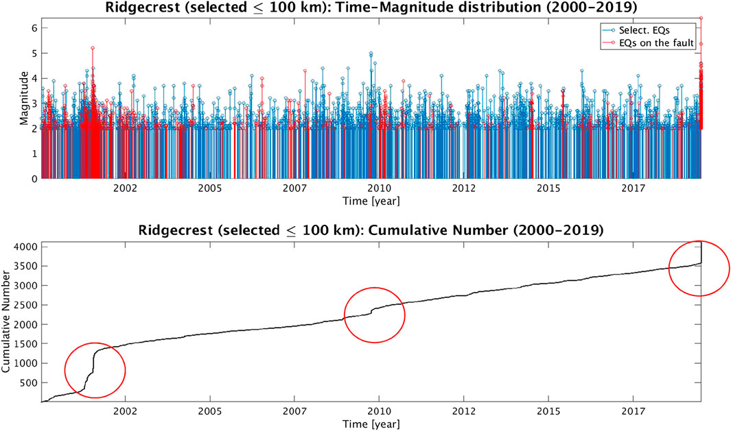
FIGURE 2. (Top) Time-magnitude distribution of the seismicity in the circular area of 100 km radius around the epicenter of the M7.1 mainshock since January 1, 2000. The earthquakes which are on the fault are indicated with red lines. (Bottom) The cumulative number of earthquakes in the same area. At least three sequences can be recognized (as evidenced by red circles): the first, a long lasting one, in 2001, where the largest magnitude exceeded M5; the second, shorter, around the beginning of 2010, whose largest magnitude slightly went beyond M4 and the last concentrated within just 2 days before the 2019 mainshock.

The Ridgecrest sequence occurred in a region with a prevailing NW-SE faulting trend, almost parallel to the more famous San Andreas Fault. The double-couple solution obtained by the U.S. Geological Survey (USGS) indicates that it could have been due to either a right NW-SE or a left NE-SW slip, the former being the more reasonable, if we consider that this fault lays approximately 150 km NE of San Andreas Fault and that the Pacific Plate moves to the NW with respect to the North America Plate (USGS, https://earthquake.usgs.gov/earthquakes/eventpage/ci38457511/executive, last visit January 08, 2020): a confirmation of that is offered by the GPS data analysis conducted by Ross et al. (2019) (please see their Supplementary Figure S13). The “pervasive orthogonal faulting” (Ross et al., 2019) of the area is the origin of a certain degree of geometric complexity: indeed, the largest foreshock was expression of the NE-SW trending fault, orthogonal to that of the M7.1 event.

In the past, around 2002, a former seismic sequence occurred almost in the same area of Ridgecrest, where the recent M7.1 seismic event has been localized (Ross et al., 2019). In order to better analyze the recent Ridgecrest seismicity, we further restricted the time and spatial intervals to those events, which occurred starting from January 1, 2000, confined by a circular area whose radius is 100 km and centered in the epicenter. The obtained catalog of the events in this circular area shows some interesting features: the plot on top of Figure 2 represents the time-magnitude distribution of the selected events where, in particular, the red color identifies all the events, which fall onto the superficial projection of the fault plane (thick white line in Figure 1); on the bottom, the cumulative number of the events is reported: it increments earthquake by earthquake, i.e., as a new earthquake occurs. It is evident that around the first half of 2001, the Ridgecrest fault area was hit by a sequence whose maximum magnitude was a bit larger than 5. Although many other events followed this sequence and rarely exceeded magnitude 4, it was only around 2010 that another shorter sequence took place: even in that case, the maximum magnitude did not exceed M4. Please note the steep accumulation of events at the end of the figure. When focusing on approximately the previous month before the mainshock to better inspect the distribution of the earthquakes (Figure 2), we can check that no significant event occurred on the fault, except for the earlier 2 days when many earthquakes, several M4+, hit the area, starting from (triggered by) the M6.4 foreshock.

One of the features of the seismic sequences is its accelerating character, i.e., the increase in the rate of earthquake occurrence, which can appear in a region before a large earthquake: this is called AMR, whose physical model promoted by Bowman et al. (1998) is based on the hypothesis that stress changes in the lithosphere lead to an increase in the rate of smaller sized earthquakes before a mainshock. Here, for clarity purpose, we give only the formulation of the quantities involved in the analysis: for a complete discussion of this topic, please refer to De Santis et al. (2015).

To take into account the cumulative effect of a series of N earthquakes at the time t of the last N-th earthquake on a fault, Benioff (1949) introduced the quantity $s\left(t\right)$, now called cumulative Benioff strain:

where the energy in Joule $E_i=\left( {10}^{1.5M_i+4.8}\right)$ of the i-th event as a function of its magnitude is involved (De Santis et al., 2015). The AMR can be estimated by looking at the power-law behavior with time of $s\left(t\right)$, as given by the following form:

where $A>0,$$B<0,$$t_f>0$, and $0<m<1$ are sequence-dependent “constant” parameters to be determined through a fit to $s\left(t\right)$ (Figure 3). In theory, $t_f$ would represent the time of failure of the earthquake fault.

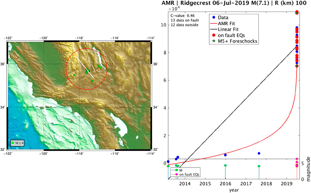
FIGURE 3. (Left) Geographical map with the M4+ earthquakes, selected since 2013.0 until the mainshock origin time, inside the 100 km radius circle for the accelerated moment release (AMR) analysis. (Right) The results of the AMR technique applied together with the temporal sequence of earthquake magnitudes. We notice an acceleration mostly occurring in the few days preceding the mainshock. Two green stars show the largest foreshocks, i.e., the M6.4 and M5.4.

A measure of presence for acceleration is the so-called C-factor (Bowman et al., 1998) defined as the ratio between the root mean square errors for the power law and the linear fit: when C < 1 significantly, then acceleration is meant to be present.

The initial time and the threshold in the minimum magnitude of earthquakes for the AMR analysis are usually a subjective choice: we preferred to be conservative and decided that 5 years of M4+ data were sufficient to detect any possible acceleration in the data. Figure 3 shows the AMR analysis applied to the events with M4+ occurred in the selected region from 2013.0 to the M7.1 origin time (excluded): blue dots represent the cumulative Benioff strain $s\left(t\right);$ the black lines and the red curve are their linear and power-law fits, respectively. We note that the power-law curve fits better data as even C-factor confirms, being well below 1 (C = 0.46). However, the most impressive fact is that the acceleration is driven by the rapid sequence of earthquakes happening just after the M6.4 foreshock, i.e., 2 days before the large event, and that most of the events occurred on the mainshock fault plane, as evidenced by the use of the red color for them.

Atmosphere

Regarding the atmosphere and how it is possibly affected by the preparation phase of the earthquake, we analyze four different parameters, i.e., skin temperature (skt), total column water vapor (tcwv), aerosol optical thickness (AOT), and methane (CH4) concentration, in an adequate region around the mainshock epicenter. Each parameter is taken at some epoch (day, year) as spatial mean of the considered region. In addition to the typical parameters that we already analyzed in previous works, such as skt and tcwv (Piscini et al., 2017) and AOT (Marchetti et al., 2019a; Marchetti et al., 2019b; Piscini et al., 2019), we also considered CH₄ since it seems a potential precursor of seismic activity from recent studies (e.g., Cui et al., 2019).

With regard to the land data, skt and tcwv have been collected from European Centre for Medium-Range Weather Forecasts (ECMWF), the meteorological European center that provides meteo-climatological observations and forecasts. The real time observations are provided in a global model called “operational archive” that is the base for the forecast. The elaboration of the measurements for long-term studies is constantly inserted in another climatological model called “Era-Interim” (ECMWF is now updating to Era-5). The year of interest has been compared to ERA-Interim historical time series. This dataset is a global atmospheric reanalysis project that uses satellite data (European remote sensing satellite, EUMETSAT, and others), input observations prepared for ERA-40, and data from ECMWF’s operational archive. Starting from January 1, 1979, it is continuously updated in real time (Dee et al., 2011). The data have been extracted with a spatial resolution of 0.5° corresponding to a resolution of around 50 km.

The AOT has been retrieved from climatological physical-chemical model MERRA-2 (Modern-Era Retrospective Analysis for Research and Applications, version 2, Gelaro et al., 2017) provided by NOAA in the sub-dataset M2T1NXAER version 5.12.4. The data have a spatial resolution of 0.625° longitude and 0.5° latitude and a temporal resolution of 1 h. For this study, the values of skt, tcwv, and AOT closer to the local midnight have been considered to avoid disturbances induced by the daily solar variability. Moreover, the data from 1980 to 2019 have been analyzed, using the data from 1980 to 2018 to construct the historical time series and 2019 to investigate the earthquake preparation phase.

The square area selected for the above three parameters is centered on the mainshock epicenter and the size is selected inside the Dobrovolsky strain radius of 10^0.43·M = 1,130 km (Dobrovolsky et al., 1979), which approximates the large-scale region where seismic precursors are usually expected around the impending faults.

The methane measurements are given as a daily product extracted from atmospheric infrared sounder (AIRS) instrument onboard NASA Earth observation system satellite Aqua provided separately for ascending and descending orbits, so the first one corresponds to daytime (1:30 PM local time at the equator) and the second one to the nighttime (1:30 AM local time at the equator). The satellite was launched into Earth’s orbit on May 4, 2002, and it is still in orbit. The instrument is based on a multispectral microwave detector (2,378 channels) that permits to monitor the atmosphere determining the surface temperature, water vapor, cloud, and overall the greenhouse gases concentrations such as ozone, carbon monoxide, carbon dioxide, and methane (Fetzer et al., 2003). In this study, we analyzed the methane volume mixing ratio data (variable CH4_VMR_D) retrieved from level 3 dataset version 6.0.9.0 from 2002 until the 2019 California earthquake only descending orbits, i.e., nighttime at about 1:30 AM. These measurements come directly from the instrument, so differently from investigated data of skt, tcwv, and AOT, the coverage depends on the orbit and so not the whole world is covered for each day. To have some data for every day, we selected an area sufficiently large, but this means to mediate different parts of the same region. For methane data, the area is smaller than the Dobrovolsky area, because it is very sensitive to anthropic activity (e.g., Le Mer and Roger, 2001). In fact, this quantity has been selected in a circle (distance of the center of the pixel from epicenter not greater than 2.0^o). As methane is a powerful greenhouse gas, we applied the “global warming” correction (see next paragraph for details).

For all parameters, we essentially applied the method CAPRI or MEANS (“MErra-2 ANalysis to search Seismic precursors” that does not include the “global warming”; see below), already introduced by Piscini et al. (2017) and Piscini et al. (2019) and applied both to seismic and volcanic hazards. These methods compare the present values of the parameter of interest with the corresponding historical time series, i.e., the background, in terms of mean and standard deviation (σ).

The CAPRI algorithm searches for anomalies in the time series of climatological parameters by a statistical analysis. Before being processed, the data are spatially averaged day-by-day selecting those over the land only by applying a land-sea mask because the sea tends to stabilize most of the atmospheric parameters (especially temperature), attenuating all eventual anomalies. Then, the algorithm removes the long-term trend over the whole day-by-day dataset mainly to remove a possible “global warming” effect, which is particularly important in skt and methane. For analogy, we removed the “global warming” effect also to tcwv data, but of course not to AOT because this parameter cannot be affected by a global warming. The data of the time series are averaged over all the years, thus obtaining the average value of a particular day over the past 40 years. Then, to make the comparison feasible, we impose the (operational archive) average value in the period analyzed to coincide with the average of the historical (ERA-Interim) time series, by a simple subtraction. Finally, an anomaly is defined when the present value overcomes the historical mean by two standard deviations. Since with both CAPRI and MEANS approaches there is an uncertainty of 1–2 days in the background, the detected anomaly should also emerge clearly such as a shift by 2–3 days (to be conservative) does not cover the data by the background.

Skin Temperature

This parameter shows three anomalies (Figure 4). We exclude the first two (blue circles) because there is not a clear emergence from the historical time series: shifting the peaks by a few days, they could be covered by the typical signal and its variations. On the other hand, the red circle indicates an evident anomaly around 25 days before the mainshock, clearly emerging by more than 2σ the historical time series. In addition, it is also characterized by a two-day persistence. The negative anomaly on around 16 March is not considered because a LAIC model expects only positive increments of temperature due to the earthquake preparation (e.g., Pulinets and Ouzounov, 2011).

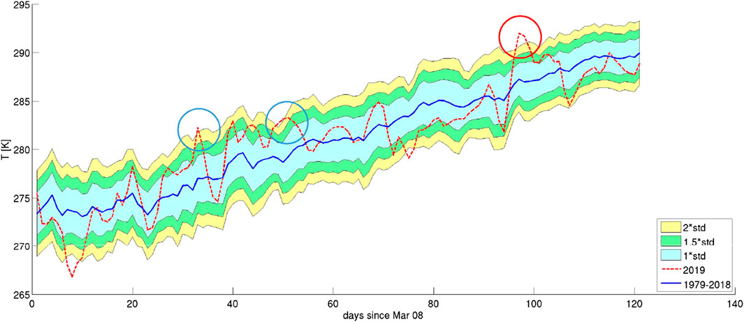
FIGURE 4. Skin temperature (skt) in the 4 months before the mainshock compared with the historical time series of the previous 40 years. The blue line is the historical mean, while the colored bands present the 1 (light blue), 1.5 (green), and 2 (yellow) standard deviations. Blue circles are anomalies that do not emerge clearly from the 2σ background, while the red circle shows a clear anomaly.

Total Column Water Vapor

For the water vapor, we can see one anomaly, which does not clearly emerge from the historical time series (Figure 5) and, in addition, it is not persistent. Hence, we consider this anomaly unlikely associated to the earthquake preparation phase.

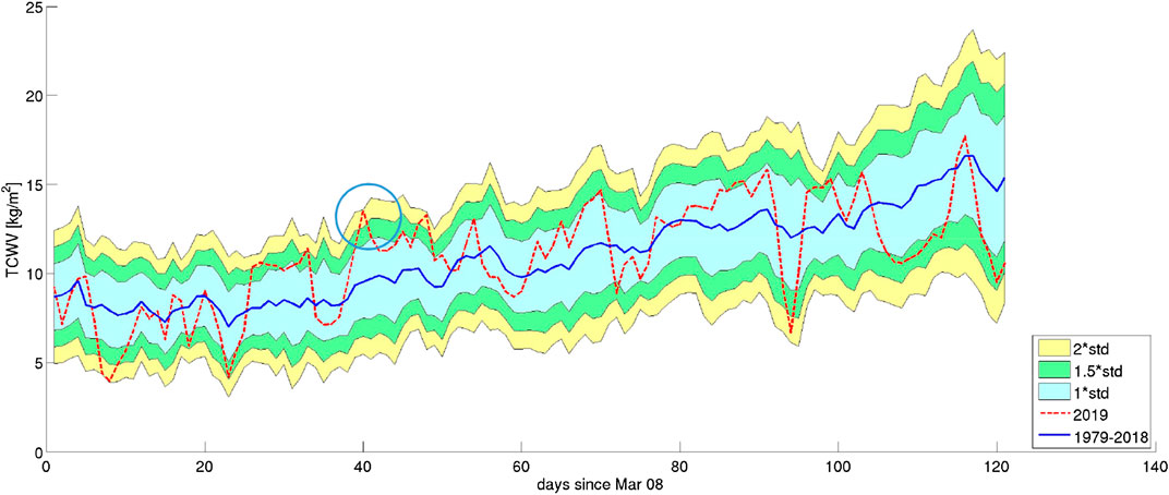
FIGURE 5. Total column water vapor (tcwv) in the 4 months before the mainshock compared with the historical time series of the previous 40 years. The blue line is the historical mean, while the colored bands present the 1 (light blue), 1.5 (green), and 2 (yellow) standard deviations. The blue circle indicates an anomaly that does not emerge clearly from the 2σ background.

Aerosol Optical Thickness

AOT is more irregular in time with respect to the two previous parameters. For this reason, we prefer to estimate the mean and standard deviation for a longer time period (6 months instead of 4). The analysis of AOT (Figure 6) shows two possible anomalies but only that one around two months before the mainshock looks more reliable: although not persistent, it clearly emerges from the overall background. In this case, the historical time series starts in 1980, because no data are available before this year. MEANS algorithm automatically excluded the 1982 and 2009 datasets because some of their values are particularly anomalous (i.e., greater than 10σ with respect to a preliminary estimation of the historical mean).

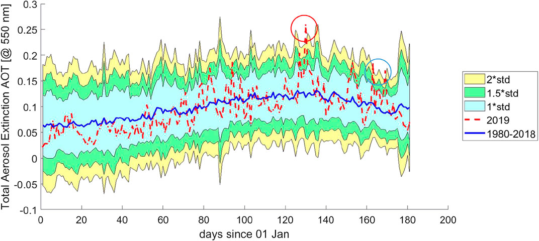
FIGURE 6. Aerosol optical thickness (AOT) in the 6 months before the mainshock, compared with the historical time series of the previous almost 40 years. The blue line is the historical mean, while the colored bands present the 1 (light blue), 1.5 (green), and 2 (yellow) standard deviations. The blue circle indicates two distinct anomalies that do not emerge clearly from the 2σ background, while the red circle shows a clear anomaly.

Methane

As for AOT, we extended the analysis to 6 months before the mainshock also for methane because it is more irregular than skt and tcwv: Figure 7 shows the analysis. Please note that the historical time series of CH₄ concentration is computed over a time interval (2002–2018) much shorter than that of the previous climatological quantities (1979–2018 for both historical skt and tcwv time series; 1980–2018 for AOT), because the methane parameter is temporally limited by the AQUA satellite availability. The first apparent CH₄ anomaly (blue circle) is not considered, because there is a close peak (by a few days) in the historical time series, so it could be within 2σ if we shift this point by 2–3 days. The second anomaly, at around 70 days from the mainshock (red circle), is considered significant instead, being clearly emerging from the 2σ band. The negative anomaly on around 15 January is not considered because a reliable LAIC model expects a release from underground sources, i.e., a positive increment due to the earthquake preparation.

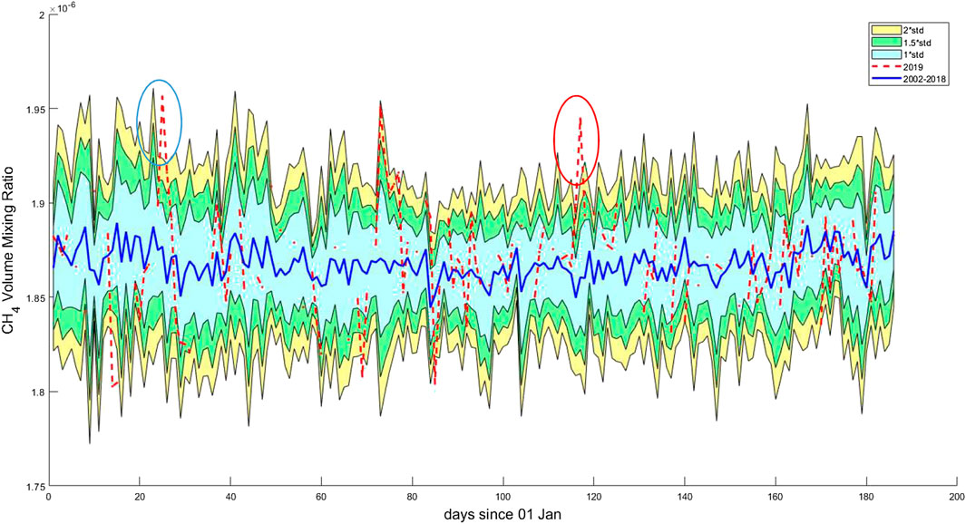
FIGURE 7. Methane (CH4) concentration in the 6 months before the mainshock compared with the historical time series of the previous almost 20 years. The blue line is the historical mean, while the colored bands present the 1 (light blue), 1.5 (green), and 2 (yellow) standard deviations. The blue circle indicates an anomaly that does not emerge clearly from the 2σ background, while the red circle shows a clear anomaly.

Ionosphere

Ionosonde

In order to search for possible pre-earthquake ionospheric anomalies, the method proposed by Korsunova and Khegai (2006) and Korsunova and Khegai (2008) and successively developed by Perrone et al. (2010), Perrone et al.(2018), and Ippolito et al. (2020) for ionosonde data was applied here. A peculiar feature of this method is the multi-ionospheric parameter approach, which takes into account the variations of sporadic E (Es) and regular F2 layers occurred simultaneously during magnetically quiet conditions (Perrone et al., 2010; Perrone et al. 2018; Ippolito et al., 2020). The occurrence of the abnormally high Es layer with Δh’Es ≥ 10 km is considered followed by an increase over 20% in f_oEs (maximum frequency of the ionogram trace associated to the Es layer) and over 10% in f_oF2 (critical frequency of the F2 layer) within one day for 2–3 h, where the variations are computed w.r.t. 27-days running medians.

Applying the method to the hourly data from the ionosonde of Point Arguello (34.7°N, 239.4°E; distant around 264 km from the epicenter), we recognize a possible pre-earthquake ionospheric anomaly from 22:00 UT on 2 June to 04:00 UT on 3 June (see Figure 8), with a significant increasing in f_oF2 at 03:00 UT on 3 June. According to the time of its occurrence, this anomaly anticipates by 5–10 h a magnetic field anomaly found by the Swarm Alpha satellite (see below and Figure 9).

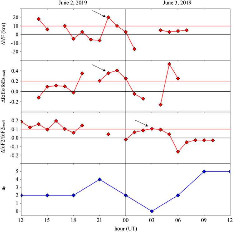
FIGURE 8. Anomaly taken from ionosonde of Point Arguello (34.7°N, 239.4°E) using observed Δh’Es, δfoEs, and δfoF2 variations (arrows). Three-hour ap geomagnetic index values are given in a lower panel. Black arrows point to possible anomalies.

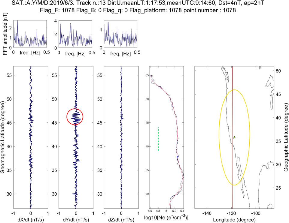
FIGURE 9. Magnetic anomaly (red circle in Y magnetic field component) taken from the Swarm Alpha satellite on June 3, 2019, at 9:14 UT (around 01 LT). From left, we show plots of dX/dt, dY/dt, and dZ/dt (i.e., the first differences of X, Y, and Z magnetic field components), the logarithm of the electron density Ne along with a green dashed line that is the Ne background level expected from the ionosonde, and finally the geographic map of the region, where the central star represents the earthquake epicenter, the yellow oval is the Dobrovolsky region, and the south-north red line indicated the satellite track projection at the Earth’s surface. Top small pictures show the FFT amplitudes for the magnetic components. First line of the heading reports the most important information about the analysis (i.e., type of satellite, date, track number, mean LT and UT, Dst, and ap magnetic indices); second line reports information about the status of satellite data flags that can reveal any problem in the satellite operations or sensor functioning.

Electron Density and Magnetic Field From Satellite

For the electron density (Ne), we considered a background based on median values from ionosonde data of hmF2 (peak true height of the F2 layer). The satellite data have been scaled at the F2 altitude by a simple proportion using the International Reference Ionosphere, IRI-2016, model (Bilitza et al., 2017) computed for both altitudes. This background was associated to a geographic cell of 5° longitude and 3° latitude centered in the ionosonde location, used to select the satellite data and compare them with the ionosonde background. For the comparison of Ne, we resorted to Swam satellite data. The Swarm mission by ESA is composed of three identical quasi-polar satellites, Alpha, Bravo, and Charlie launched on November 22, 2013, with a multisensor payload: among them, magnetometers and Langmuir probes (Friis-Christensen et al., 2006). Alpha and Charlie fly almost in parallel at around 460 km of altitude, while Bravo flies at around 510 km (in an almost 90° phase orbit in longitude at the epoch of Ridgecrest earthquake). One of the most interesting results was obtained during the comparison of the background Ne value of the ionosonde with that measured by the Swarm Alpha satellite (Figure 9). During the satellite passage over the same cell of the ground ionosonde on 3 June at 09:14 UT (i.e., around 01 LT), we obtained a relative variation of 1.94, i.e., the Ne value measured by the satellite is almost double w.r.t. the background (the latter has been represented in Figure 9 as a green dashed line extended in latitude for 5° around Pt. Arguello ionosonde location).

Following recent works (e.g., De Santis et al., 2017), a magnetic anomaly from the satellite can be defined from first differences, comparing the root mean square (rms) over a 3°-latitude window with respect to the analogous RMS of the whole satellite track within ±50° geomagnetic latitude. An interesting result is shown in Figure 9 (in this case rms>2.5 RMS for the window highlighted by red circle). During the same orbit when we detected the Ne anomaly, a clear anomaly in Y (East) component of the magnetic field (actually first differences in nT/s are shown) was recorded by the Swarm Alpha satellite on 3 June at 09:14 UT, when the external magnetic field was negligible (magnetic indices Dst = 4 nT and a_p = 2 nT). We notice that the track is almost along the epicenter longitude and the anomaly is located northward in latitude with respect to the epicenter. The anomaly has been recorded in nighttime, and in the same moment, the absolute value of Ne was about the double of the typical one (as shown by the green dashed line in Figure 9). The anomalous features of the magnetic and plasma measurements of Swarm for this track cannot be simply explained by typical ionospheric disturbances. Therefore, we suggest the preparation of the seismic event as a possible source for these phenomena.

As an alternative technique for magnetic field anomaly detection, the residual values, with respect to the recently updated international geomagnetic reference model IGRF-13 (https://www.ngdc.noaa.gov/IAGA/vmod/), have been calculated. Y (East) component of geomagnetic field measured by Swarm Alpha, Bravo, and Charlie satellites has been systematically inspected over the 6 months before the mainshock (this time interval is useful to have sufficiently robust statistics). A three-degree polynomial has been also further subtracted after the removal of the model in order to clean the time series from the seasonal or magnetospheric variations, not predicted by the model.

As in Akhoondzadeh et al. (2018) and Akhoondzadeh et al. (2019), we estimate a median over the 6 months before the mainshock together with the corresponding interquartile (IQR). We then define an anomaly when the residual overcomes the median by more than 1.25 IQR, by at least 1 nT, and the possible effect of the external magnetic fields can be neglected (i.e., the magnetic indices are very low: |Dst| ≤ 20 nT and a_p ≤ 10 nT). We prefer to use IQR instead of standard deviation because ionospheric magnetic signals are expected non-Gaussian. However, by analogy, the choice of this threshold would correspond for a Gaussian signal to the largest threshold of 2σ applied in the previous analyses.

Although the threshold is constant for the analyzed 6 months, please note that, before computing it, we removed the daily variation by daily median and the seasonal trend by a polynomial fit. So, after this data processing, the residuals are not anymore affected by daily or seasonal variations.

The disturbed days are automatically excluded from the graph. Three days are particularly anomalous (Figure 10): January 31, 2019 (+3.1 nT more than the upper threshold), April 26, 2019 (+2.8 nT above the upper threshold), and June 12, 2019 (−3.3 nT down the lower threshold). Another anomalous day is April 29, 2019 (+1.0 nT).

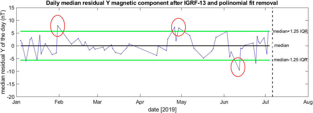
FIGURE 10. Daily median anomaly taken from Y magnetic field of all Swarm satellites with respect to IGRF-13 model predictions. We underline only the most significant anomalies with red circles. The vertical dashed line represents the mainshock occurrence.

The same time series analysis has been also applied to the scalar intensity of magnetic field F measured by Swarm (Figure 11). The residuals depict some days as clearly anomalous (also here at least 1 nT larger than the adopted threshold): June 3, 2019 (+6.2 nT), June 5, 2019 (−7.3 nT), June 12, 2019 (+1.4 nT), June 16, 2019 (−13.7 nT), June 22, 2019 (+1.7 nT), June 24, 2019 (−9.1 nT), June 27, 2019 (−8.9 nT), June 30, 2019 (+2.6 nT), and July 3, 2019 (+2.8 nT). We notice that June 12, 2019, is extracted as anomalous by both Y and F analyses. It is interesting to note that in the last period (around one month) approaching the earthquake, the residuals of the magnetic field intensity present more anomalies (highlighted by large red ovals in the figure).

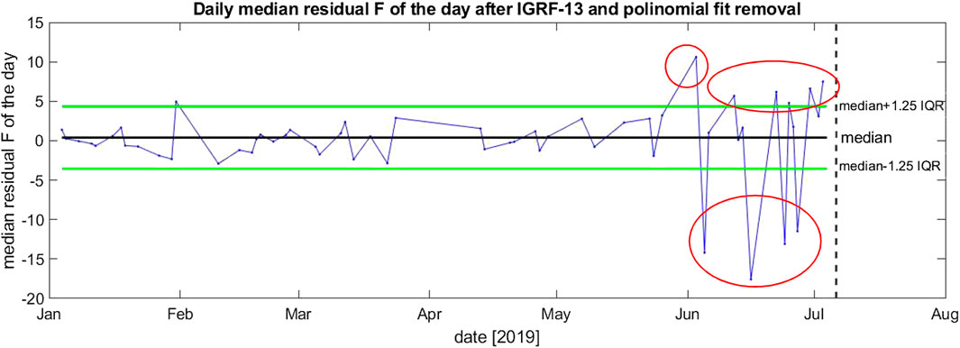
FIGURE 11. Daily median anomaly taken from total intensity F of all Swarm satellites with respect to IGRF-13 model predictions. Periods of anomalies are evidenced by red circles. The vertical dashed line represents the mainshock occurrence.

Discussion and Conclusion

Table 1 summarizes the occurrence of all anomalies (dubious anomalies are within a square bracket). It is interesting to highlight that our found precursor times are much longer than those identified by many other papers on earthquake precursors, especially ionospheric precursors, which seem to occur only a few hours to days before large earthquakes (e.g., Heki, 2011; He and Heki, 2017; Yan et al., 2017). Indeed, our recent works highlight a preparation time much longer than few days (e.g., Liu et al., 2020; Marchetti et al., 2019a; Marchetti et al., 2019b). These longer precursor times could be attributed to the long-term process of earthquake preparation (Sugan et al., 2014; Di Giovambattista and Tyupkin, 2004). Moreover, our recent results turned out to be in agreement with the empirical Rikitake (1987) law, recently confirmed for ionospheric precursors from the satellite by De Santis et al. (2019c), which also provide a reasonable physical explanation for the law itself. In accordance to this law, where the precursor time depends on the earthquake magnitude (i.e., the greater the magnitude, the longer the precursor time), Rikitake (1987) estimated an anticipation time from 32 days (radon) to some years for the seismicity precursor of a M7.1 earthquake. It should also be considered that the distance of the monitoring site to the earthquake epicenter could also be important for land-based observations. In fact, it is expected that with a shorter distance, the precursory time is usually longer (Sulthankhodaev, 1984). Therefore, precursory anomalies of only hours to days are not frequent. Inan et al. (2010) mention precursory hydrogeochemical anomalies in Western Turkey lasting for more than a month before an earthquake magnitude 4.8; the epicenter was within few tens of kilometers to the observation site. The ground water level data we provide from a borehole located some 200 km distant from the epicenter (Figure 12) also show a precursory anomaly lasting almost a year (between September 2018 and July 2019). Another important point is to check whether previous researches investigated or not a long time in advance with respect to the seismic event. For example, DEMETER data investigation (e.g., Yan et al., 2017, which is the last statistic study on EQs-DEMETER) has explored only from 15 days before each earthquake. In De Santis et al. (2019c), published by most of the authors of this article, the DEMETER results with anticipation time around 6 days were confirmed, also giving evidences of the existence of possible longer time precursors, for example, 80 days before the seismic event or even some hundred days before for higher magnitude seismic events, which is in accordance to the Rikitake law. On the other hand, some ionospheric precursors have been also registered up to some months in advance (middle-term precursors) (Sidorin, 1979; Korsunova and Khegai, 2006; Korsunova and Khegai, 2008; Hao et al., 2000; Perrone et al., 2010; Perrone et al., 2018), confirming our present results.

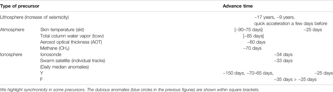
TABLE 1. Type of precursor and corresponding advance time(s).

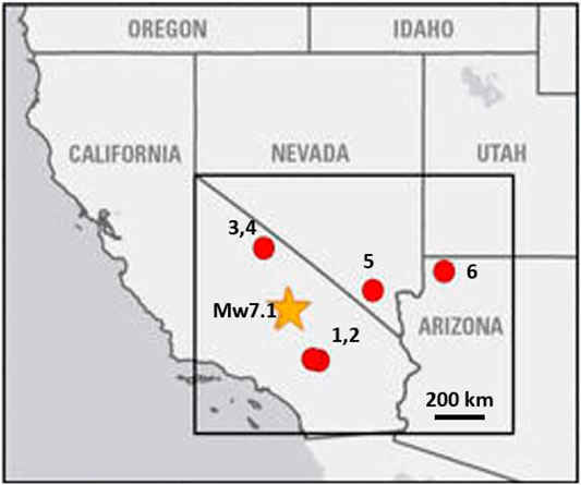
FIGURE 12. Locations of the epicenter of the July 6, 2019, M7.1 Ridgecrest earthquake and six USGS groundwater-monitoring sites. The monitoring sites shown are California 1) 002S002W02F002S, 2) 002S002W12H001S, 3) 003S027E25N001M, and 4) 003S029E30E002M; Nevada 5) 212 S19 E61 19BC 1 CNLV Deer Springs; and, Arizona 6) B-40-04 06AAC1 [Kaibab-Paiute Well] (USGS 2019).

From the overall results of our study, the atmosphere looks very sensitive to the preparation of the impending earthquake and the anomalies tend to concentrate in a few occasions, from three months to almost one before the mainshock. The ionosphere (from ionosonde and Swarm satellite data analysis) provides anomalous signals from five months before the mainshock and then at around 2 months before. It then clearly depicts 2–3 June 2019 as a disturbed period in both ionosonde and satellite, during very quiet geomagnetic conditions. The high compatibility of the anticipation time and distance of the ionosonde with respect to the future epicenter of the earthquake using the Korsunova and Khegai (2006) and Korsunova and Khegai (2008) method can strongly support the hypothesis that this feature is induced by the earthquake preparation processes, e.g., release of ionized particles from the lithosphere (see Freund, 2011; Pulinets and Ouzounov, 2011; Hayakawa et al., 2018), before the Ridgecrest major earthquakes.

We can now attempt to consider all anomalies in a unique framework. Particularly powerful is to estimate a cumulative curve of all anomalies together (actually excluding the seismic ones, already included in the AMR fit). When we plot the cumulative number of anomalies (Figure 13), we find that a power-law fits the data points very well, much better than a straight line (we fixed the m-exponent of the power law as that typical of a critical system, i.e., m = 0.25). This can be measured by the analogous C-factor, already introduced for AMR, i.e., the ratio between the root mean square of the power-law fit w.r.t. the same of the straight line (Bowman et al., 1998). We estimate for this latter cumulate C = 0.49, which means a clear acceleration of all the anomalies: by the way, it is interesting that the value of this latter C-factor is almost the same as the one calculated for the AMR, producing a similar conclusion obtained for the M7.8 Nepal 2015 case study comparing seismic and magnetic anomaly patterns by De Santis et al. (2017). Therefore, from Figure 13, we can affirm that the anomalies tend to accelerate as the earthquake is approaching, pointing to the time of occurrence with a small uncertainty of only few days (±3 days). Inclusion of the few dubious anomalies (blue circles in the figures of analyses) does not change the overall result significantly. Ground-based precursory anomaly, for verification of our results, was sought and only borehole water level data have been found available from the USGS open access database. USGS reported in October 2019 (USGS, 2019) that oscillatory changes were recorded in short-term water levels of some boreholes varying in distance to the epicenter of the M7.1 earthquake from about 200 to 400 km (Figure 12). We downloaded the data for all six borehole locations for a time interval of 4 years (from January 1, 2016, to January 1, 2020) in order to assess the background level and evaluate pre-seismic anomalies, if any. Time series of the water level recorded in one borehole (#2) located about 200 km to the south of the epicenter is given in Figure 14. Data from other five boreholes did not enable robust evaluation with respect to seismicity (these can be viewed from USGS, (2019)): we explain this fact because one station (#6) is too far from the epicentral region, while the others (#1, #3, #4, and #5) do not show any pre-earthquake anomaly because of the stress anisotropy and/or block boundaries hindering stress transfer to localities of these stations (similar effects are discussed by Inan et al., 2012). In Figure 14, gradual shallowing trend in the water level is apparent until about September 2018 (about 9 months before the mainshock) when disturbance in the data started and the water level started to gradually decrease until July 6, 2019. After that, the water level has gradually increased again. An anomaly at 270 days before the mainshock is suggested by the data. Using Sultankhodhaev’s (1984) empirical formula, relating the time T (in days) of the anomaly, the distance D (in km) of its location w.r.t. the mainshock epicenter, and the earthquake magnitude M

we calculated an expected anomaly anticipation time of 105 days as in this case D = 200 km and M = 7.1. The apparent anomaly anticipation time (270 days) from Figure 14 and theoretical expected anticipation time (105 days) from the empirical approach correlate well with anomalies detected based on magnetic and ionospheric data as listed in Table 1.

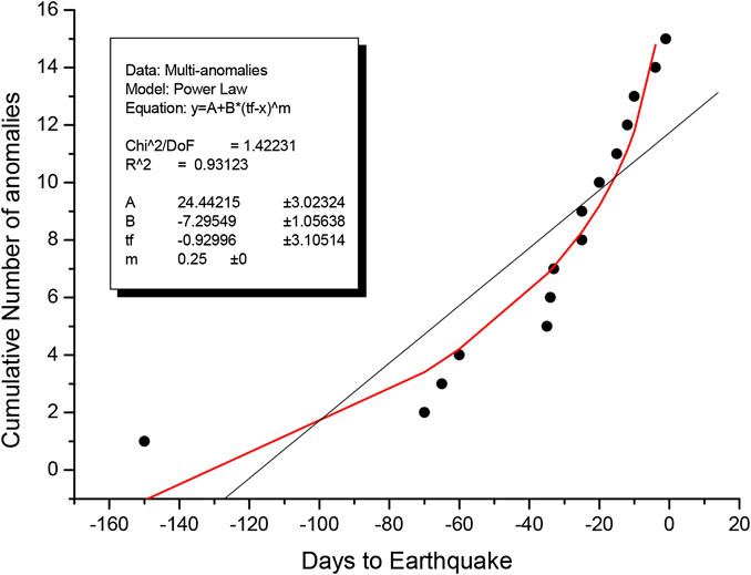
FIGURE 13. Cumulative number of all clear anomalies (indicated here as black circles; here, we do not consider the lithospheric anomalies of seismicity, already counted in AMR). Time origin t = 0 is themainshock occurrence. Red fit is a power law while the black is a straight line. As for AMR, also here can be estimated the C-factor, C = 0.49, which confirms a strong acceleration as the mainshock is approaching.

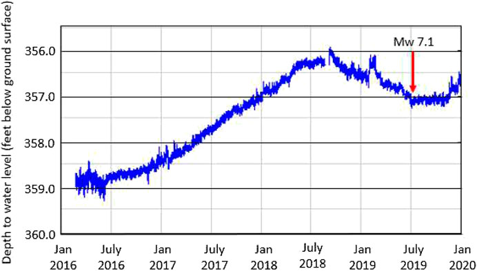
FIGURE 14. Water level for about 4 years (3.5 years before and half year after the Ridgecrest mainshock) at location #2 (see Figure 12 for location) (USGS report of October 2019). Disturbance of the water level in September 2018 is followed by gradual decrease of cumulative of about one foot (30.5 cm) until the day of the Ridgecrest mainshock. A peak representing a few weeks in February 2019 (about 5 months) prior to earthquake is also noteworthy.

From different analyses of seismic, atmospheric, and ionospheric data, as well as limited ground-based observations, we find a chain of processes from the ground to atmosphere and ionosphere. We can safely conclude that this series of anomalous events in the different geolayers (lithosphere where the earthquake occurs, atmosphere, and ionosphere) is probably activated by the preparation phase of the Ridgecrest earthquake.

Data Availability Statement

Publicly available datasets were analyzed in this study. These data can be found in USGS Seismic Catalogue, ESA Swarm, ECMWF, and MERRA-2, data Portals.

Author Contributions

ADS was responsible for the design and organization of the work, bibliography search, some data analyses and drawing of a few figures, writing the first draft of the article, and editing the final version. GC was involved in the bibliography search, data analyses and preparation of some figures, and editing for the final version. DM, AP, DS, LP, SAC, and SI were involved in the data analyses and preparation of a few figures, and editing the final version.

Funding

This work was undertaken in the framework of the European Space Agency (ESA)-funded project SAFE (Swarm for earthquake study) 4000116832/15/NL/MP, while Agenzia Spaziale Italiana (ASI) funded project LIMADOU-Scienza n. 2016-16-H0. Part of the work has been made also under the project ISSI-BJ “The electromagnetic data validation and scientific application research based on CSES satellite.”

Conflict of Interest

The authors declare that the research was conducted in the absence of any commercial or financial relationships that could be construed as a potential conflict of interest.

References

Akhoondzadeh, M., De Santis, A., Marchetti, D., Piscini, A., and Cianchini, G. (2018). Multi precursors analysis associated with the powerful Ecuador (MW = 7.8) earthquake of 16 April 2016 using Swarm satellites data in conjunction with other multi-platform satellite and ground data, Adv. Space Res. 61, 248–263. doi:10.1016/j.asr.2017.07.014
Akhoondzadeh, M., De Santis, A., Marchetti, D., Piscini, A., and Jin, S. (2019). Anomalous seismo-LAI variations potentially associated with the 2017 Mw = 7.3 Sarpol-e Zahab (Iran) earthquake from Swarm satellites, GPS-TEC and climatological data. Adv. Space Res. 64, 143–158. doi:10.1016/j.asr.2019.03.020
Barnhart, W. D., Hayes, G. P., and Gold, R. D. (2019). The July 2019 Ridgecrest, California, earthquake sequence: kinematics of slip and stressing in cross‐fault ruptures. Geophys. Res. Lett. 46, 11859–11867. doi:10.1029/2019gl084741
Bilitza, D., Altadill, D., Truhlik, V., Shubin, V., Galkin, I., Reinisch, B., et al. (2017). International Reference Ionosphere 2016: from ionospheric climate to real-time weather predictions. Space Weather 15, 418–429. doi:10.1002/2016SW001593
Bowman, D. D., Ouillon, G., Sammis, C. G., Sornette, A., and Sornette, D. (1998). An observational test of the critical earthquake concept. J. Geophys. Res. 103, 24359–24372. doi:10.1029/98jb00792
Bulut, F. (2015). Different phases of the earthquake cycle captured by seismicity along the North Anatolian Fault. Geophys. Res. Lett. 42, 2219–2227. doi:10.1002/2015gl063721
Chen, K., Avouac, J.-P., Aati, S., Milliner, C., Zheng, F., and Shi, C. (2020). Cascading and pulse-like ruptures during the 2019 ridgecrest earthquakes in the Eastern California shear zone. Nat. Commun. 11, 22. doi:10.1038/s41467-019-13750-w
Cianchini, G., De Santis, A., Giovambattista, R. D., Abbattista, C., Amoruso, L., Campuzano, S. A., et al. . (2020). Revised accelerated moment release under test: fourteen worldwide real case studies in 2014–2018 and simulations. Pure Appl. Geophys. 177, 4057–4087. doi:10.1007/s00024-020-02461-9
Cui, J., Shen, X., Zhang, J., Ma, W., and Chu, W. (2019). Analysis of spatiotemporal variations in middle-tropospheric to upper-tropospheric methane during the Wenchuan Ms = 8.0 earthquake by three indices. Nat. Hazards Earth Syst. Sci. 19, 2841–2854. doi:10.5194/nhess-19-2841-2019
De Santis, A. (2009). “Geosystemics,” in Proceedings of the 3rd IASME/WSEAS international conference on geology and seismology (GES’09), Cambridge, UK, 21–26 February 2009, 36–40.
De Santis, A. (2014). “Geosystemics, Entropy and criticality of earthquakes: a vision of our planet and a key of access,” in Addressing global environmental security through innovative educational curricula. (Basingstoke, United Kingdom: Springer Nature), 3–20.
De Santis, A., Cianchini, G., and Di Giovambattista, R. (2015). Accelerating moment release revisited: examples of application to Italian seismic sequences. Tectonophysics 639, 82–98. doi:10.1016/j.tecto.2014.11.015
De Santis, A., Balasis, G., Pavón-Carrasco, F. J., Cianchini, G., and Mandea, M. (2017). Potential earthquake precursory pattern from space: the 2015 Nepal event as seen by magnetic Swarm satellites. Earth Planet Sci. Lett. 461, 119–126. doi:10.1016/j.epsl.2016.12.037
De Santis, A., Abbattista, C., Alfonsi, L., Amoruso, L., Campuzano, S. A., Carbone, M., et al. (2019a). Geosystemics view of earthquakes. Entropy 21 (4), 412. doi:10.3390/e21040412
De Santis, A., Marchetti, D., Spogli, L, Cianchini, G., Pavón-Carrasco, F. J., Franceschi, G. D., et al. . (2019b). Magnetic field and electron density data analysis from Swarm satellites searching for ionospheric effects by great earthquakes: 12 case studies from 2014 to 2016. Atmosphere 10, 371. doi:10.3390/atmos10070371
De Santis, A., Marchetti, D., Pavón-Carrasco, F. J., Cianchini, G., Perrone, L., Abbattista, C., et al. (2019c). Haagmans, Precursory worldwide signatures of earthquake occurrences on Swarm satellite data. Sci. Rep. 9, 20287. doi:10.1038/s41598-019-56599-1
Dee, D. P., Uppala, S. M., Simmons, A. J., Berrisford, P., Poli, P., Kobayashi, S., et al. (2011). The ERA-Interim reanalysis: configuration and performance of the data assimilation system. Q. J. R. Meteorol. Soc. 137, 553–597. doi:10.1002/qj.828
Di Giovambattista, R., and Tyupkin, Y. S. (2004). Seismicity patterns before the M=5.8 2002, Palermo (Italy) earthquake: seismic quiescence and accelerating seismicity. Tectonophysics 384 (1-4), 243–255. doi:10.1016/j.tecto.2004.04.001
Dobrovolsky, I. P., Zubkov, S. I., and Miachkin, V. I. (1979). Estimation of the size of earthquake preparation zones. PAGE, 117, 1025–1044. doi:10.1007/bf00876083
Fetzer, E., McMillin, L. M., Tobin, D., Aumann, H. H., Gunson, M. R., McMillan, W. W., et al. (2003). Airs/amsu/hsb validation, geoscience and Remote sensing. IEEE Transactions 41 (2), 418–431. doi:10.1109/tgrs.2002.808293
Freund, F. (2011). Pre-earthquake signals: underlying physical processes. J. Asian Earth Sci. 41, 383–400. doi:10.1016/j.jseaes.2010.03.009
Freund, F. (2013). Earthquake forewarning—a multidisciplinary challenge from the ground up to space. Acta Geophysica 61 (4), 775–807. doi:10.2478/s11600-013-0130-4
Friis-Christensen, E., Luhr, H., and Hulot, G. (2006). Swarm: a constellation to study the Earth’s magnetic field. Earth Planet. Space 58, 351–358. doi:10.1186/bf03351933
Gelaro, R., McCarty, W., Suárez, M. J., Todling, R., Molod, A., Takacs, L., et al. (2017). The Modern-Era retrospective analysis for research and applications, version 2 (MERRA-2), American meteorological society - modern-Era retrospective analysis for research and applications version 2 (MERRA-2) special collection. J. Climate 30, 5419--5454. doi:10.1175/JCLI-D-16-0758.1
Hao, J., Tianming, T., and Li, D. (2000). Progress in the research of atmospheric electric field anomaly as an index for short-impending prediction of earthquakes. J. Earthquake Prediction Res. 8, 241–255. doi:10.1007/BF02650462
Hayakawa, M., Asano, T., Rozhnoi, A., and Solovieva, M. (2018). “Very-low- and low-frequency sounding of ionospheric perturbations and possible association with earthquakes,” in Pre-earthquake Processes: a multidisciplinary approach to earthquake prediction studies. Editors D. Ouzounov, et al. . (New York, NY: AGU Book, Wiley), 277–304.
He, L., and Heki, K. (2017). Ionospheric anomalies immediately before Mw7.0–8.0 earthquakes. J. Geophys. Res. Space Phys. 122, 8659–8678. doi:10.1002/2017ja024012
Heki, K. (2011). Ionospheric electron Enhancement preceding the 2011 tohoku-oki earthquake. Geophys. Res. Lett. 38 (17), 1–5. doi:10.1029/2011gl047908
Ippolito, A., Perrone, L., De Santis, A., and Sabbagh, D. (2020). Ionosonde data analysis in relation to the 2016 central Italian earthquakes. Geosciences 10, 354. doi:10.3390/geosciences10090354
İnan, S., Ertekin, K., Seyis, C., Şimşek, Ş., Kulak, F., Dikbaş, A., et al. . (2010). Multi-disciplinary earthquake researches in Western Turkey: hints to select sites to study geochemical transients associated to seismicity. Acta Geophysica 58, 767–813. doi:10.2478/s11600-010-0016-7
İnan, S., Pabuccu, Z., Kulak, F., Ergintav, S., Tatar, O., Altunel, E., et al. . (2012). Microplate boundaries as obstacles to pre-earthquake strain transfer in Western Turkey: inferences from continuous geochemical monitoring. J. As. Earth Sc. 48, 56–71. doi:10.1016/j.jseaes.2011.12.016
Korsunova, L. P., and Khegai, V. V. (2006). Medium-term ionospheric precursors to strong earthquakes. Int. J. Geomagn. Aeron. 6, GI3005, doi:10.1029/2005gi000122
Korsunova, L. P., and Khegai, V. V. (2008). Analysis of seismo-ionospheric disturbances at the chain of Japanese stations for vertical sounding of the ionosphere. Geomagn. Aeron. 48, 392–399. doi:10.1134/s0016793208030134
Le Mer, J., and Roger, P. (2001). Production, oxidation, emission and consumption of methane by soils: a review. Eur. J. Soil Biol. 37, 25–50. doi:10.1016/s1164-5563(01)01067-6
Liu, Q., De Santis, A., Piscini, A., Cianchini, G., Ventura, G., and Shen, X. (2020). Multi-parametric climatological analysis reveals the involvement of fluids in the preparation phase of the 2008 Ms 8.0 wenchuan and 2013 Ms 7.0 lushan earthquakes. Rem. Sens. 12, 1663. doi:10.3390/rs12101663
Marchetti, D., De Santis, A., D’Arcangelo, S., Poggio, F., Piscini, A., Campuzano, A., et al. . (2019a). Pre-earthquake chain processes detected from ground to satellite altitude in preparation of the 2016–2017 seismic sequence in Central Italy. Remote Sens. Environ. 229, 93–99. doi:10.1016/j.rse.2019.04.033
Marchetti, D., De Santis, A., Shen, X., Campuzano, S. A., Perrone, L., Piscini, A., et al. . (2019b). Possible Lithosphere-Atmosphere-Ionosphere Coupling effects prior to the 2018 Mw=7.5 Indonesia earthquake from seismic, atmospheric and ionospheric data. J. Asian Earth Sci. 188, 104097. doi:10.1016/j.jseaes.2019.104097
Marchetti, D., De Santis, A., D’Arcangelo, S., Poggio, F., Jin, S., Piscini, A., et al. (2020). Magnetic field and electron density anomalies from Swarm satellites preceding the major earthquakes of the 2016–2017 Amatrice-Norcia (Central Italy) seismic sequence. Pure Appl. Geophys. 177, 305–319. doi:10.1007/s00024-019-02138-y
Perrone, L., Korsunova, L. P., and Mikhailov, A. V. (2010). Ionospheric precursors for crustal earthquakes in Italy. Ann. Geophys. 28, 941–950. doi:10.5194/angeo-28-941-2010
Perrone, L., De Santis, A., Abbattista, C., Alfonsi, L., Amoruso, L., Carbone, M., et al. (2018). Ionospheric anomalies detected by ionosonde and possibly related to crustal earthquakes in Greece. Ann. Geophys. 36, 361–371. doi:10.5194/angeo-36-361-2018
Piscini, A., De Santis, A., Marchetti, D., and Cianchini, G. (2017). A multi-parametric climatological approach to study the 2016 Amatrice-Norcia (Central Italy) earthquake preparatory phase. Pure Appl. Geophys. 174 (10), 3673–3688. doi:10.1007/s00024-017-1597-8
Piscini, A., Marchetti, D., and De Santis, A. (2019). Multi-parametric climatological analysis associated with global significant volcanic eruptions during 2002–2017. Pure Appl. Geophys. 176, 3629–3647. doi:10.1007/s00024-019-02147-x
Pulinets, S., and Ouzounov, D. (2011). Lithosphere–atmosphere–ionosphere coupling (LAIC) model—an unified concept for earthquake precursors validation. J. Asian Earth Sci. 41 (4–5), 371–382. doi:10.1016/j.jseaes.2010.03.005
Rikitake, T. (1987). Earthquake precursors in Japan: precursor time and detectability. Tectonophysics 136, 265–282. doi:10.1016/0040-1951(87)90029-1
Ross, Z. E., Idini, B., Jia, Z., Stephenson, O. L., Zhong, M., Wang, X., et al. . (2019). Hierarchical interlocked orthogonal faulting in the 2019 Ridgecrest earthquake sequence. Science 366, 346–351. doi:10.1126/science.aaz0109
Rymer, M. J., Langenheim, V. E., and Hauksson, E. (2002). The hector mine, California, earthquake of 16 october 1999: introduction to the special issue. Bull. Seismol. Soc. Am. 92 (4), 1147–1153. doi:10.1785/0120000900
Sidorin, A. Y. (1979). The dependence of the time of appearance of earthquake precursors on the epicenter distance. Proc. Acad. Sci. USSR 25 (4), 825 [in Russian].
Sobolev, G. A., Huang, Q., and Nagao, T. (2002). Phases of earthquake’s preparation and by chance test of seismic quiescence anomaly. J. Geodyn. 33, 413–424. doi:10.1016/s0264-3707(02)00007-8
Sugan, M., Kato, A., Miyake, H., Nakagawa, S., and Vuan, A. (2014). The preparatory phase of the 2009 Mw 6.3 L’Aquila earthquake by improving the detection capability of low-magnitude foreshocks. Geophys. Res. Lett. 41, 6137–6144. doi:10.1002/2014GL061199
USGS (2019). The ups and downs of groundwater levels after the july 2019 ridgecrest, CA earthquakes. Available at: https://www.usgs.gov/center-news/ups-and-downs-groundwater-levels-after-july-2019-ridgecrest-ca-earthquakes. (Accessed October, 2019).
Keywords: earthquake, lithosphere-atmosphere-ionosphere coupling, multiparametric approach, earthquake precursor anomalies, earthquake preparation process
Citation: De Santis A, Cianchini G, Marchetti D, Piscini A, Sabbagh D, Perrone L, Campuzano SA and Inan S (2020) A Multiparametric Approach to Study the Preparation Phase of the 2019 M7.1 Ridgecrest (California, United States) Earthquake. Front. Earth Sci. 8:540398. doi: 10.3389/feart.2020.540398
Received: 04 March 2020; Accepted: 25 September 2020;
Published: 24 November 2020.
Edited by:
Giovanni Martinelli, National Institute of Geophysics and Volcanology, ItalyReviewed by:
Michael Emmanuel Contadakis, Aristotle University of Thessaloniki, GreeceJing Liu, China Earthquake Administration, China
Copyright © 2020 De Santis, Cianchini, Marchetti, Piscini, Sabbagh, Perrone, Campuzano and Inan. This is an open-access article distributed under the terms of the Creative Commons Attribution License (CC BY). The use, distribution or reproduction in other forums is permitted, provided the original author(s) and the copyright owner(s) are credited and that the original publication in this journal is cited, in accordance with accepted academic practice. No use, distribution or reproduction is permitted which does not comply with these terms.
*Correspondence: Angelo De Santis, angelo.desantis@ingv.it
†Present address: Saioa Arquero Campuzano, Instituto de Geociencias IGEO (CSIC-UCM), Madrid, Spain
Sedat Inan, Faculty of Mines, Department of Geological Engineering, Istanbul Technical University, Istanbul, Turkey