Chemometric Modeling of Trace Element Data for Origin Determination of Demantoid Garnets


1
North Bavarian NMR-Centre, University of Bayreuth, 95447 Bayreuth, Germany
2
Institute for Chemical Technology of Organic Materials, Johannes Kepler Univeristy Linz, 4040 Linz, Austria
*
Author to whom correspondence should be addressed.
Minerals 2020, 10(12), 1046; https://doi.org/10.3390/min10121046
Submission received: 21 October 2020
/
Revised: 20 November 2020
/
Accepted: 22 November 2020
/
Published: 24 November 2020
(This article belongs to the Special Issue Analytical Tools to Constrain the Origin of Minerals)
Abstract
:The determination of country of origin poses a common problem in the appraisal of gemstones and is in many cases still based on the observation of inclusions and growth features of a gem, whereas chemical analysis is only done by major labs. We have used Laser Ablation Inductively Coupled Plasma Mass Spectrometry to analyze the trace element profiles of demantoid garnets from six different countries and identified a set of six elements, which are magnesium, aluminum, titanium, vanadium, chromium, and manganese, that are necessary to assign the mining regions with a good certainty. By using the logarithms of the trace element concentrations and subjecting them to chemometric modeling, we were able to separate the demantoids originating from Russia, Pakistan, Namibia, Iran, and Madagascar very well, leaving only Italy with some uncertainty. Results are presented for an “all origins” model as well as pair-wise comparison of two locations at a time, which lead to even better results.
Keywords:
multivariate statistics; chemometrics; origin determination; garnets; demantoid; LA-ICP-MS1. Introduction
The correct determination of origin of gemstones has gained more and more importance recently. The desire to know where a gem comes from is not only scientifically driven but to a very large extent by the trade. For a scientist it might be hard to understand that for example two blue sapphires, which have the same size, weight, color, clarity and cut are appraised differently only because they hail from different sources. The trade, however, introduces factors such as rarity and history into the appraisal process and thus the blue sapphire originating from e.g., Madagascar (currently producing) will be less valuable than the one that has been found in the famed Kashmir region (found in 1881 after a landslide and now exhausted) [1,2]. Additionally, ethical issues associated with gemstone production are becoming increasingly important. Hence, it will be necessary in certain cases to prove that gems do not come from conflict areas as those might be banned from trade in some countries, such as jade and rubies originating from Burma which were banned in the United States from 2008 to 2016.
In classical gemology, mainly optical characteristics have been used to determine origins, and above all, inclusions. Tiny crystals which grew in the host gem material are dependent on the geological setting and thus provide a good tool to eliminate certain sources. For instance, in sapphires it is possible to assign certain origins by identifying inclusions [3]. However, the fact that inclusions are not always present, especially in high-priced gemstones, renders this approach problematic. In the last decades, to optimize the inclusion-based process, major labs have started to exploit more advanced technologies, among them the determination of chemical composition. By determining major and minor elements conclusions about e.g., sapphire genesis can be drawn, or the origin of copper bearing (Paraiba-type) tourmalines be determined [4]. The analytical arsenal used today includes techniques such as X-ray fluorescence (XRF), laser induced breakdown spectroscopy (LIBS), or laser ablation inductively coupled plasma mass spectrometry (LA-ICP-MS). Each of these technologies has its merits but also weaknesses: whereas XRF gives robust values for major elements, the other two techniques focus on trace elements. Having the lowest detection limits, typically in the ppb range, LA-ICP-MS further exhibits an excellent linearity of up to eight orders of magnitude. By contrast, higher concentrations very often present a problem for this technique. However, having access to both, major components as well as trace elements, is desirable for obtaining the overall chemical composition in a greater context.
In our study we have focused on the determination of geographic origin of demantoids, which is the well accepted trade name of the green variety of andradite (Ca3Fe2(SiO4)3) garnets. Demantoids have first been found in the Russian Urals in the river Bobrovka near the village Elizavetinskoye, close to Niznij Tagil (or often just called Tagil) in the middle of the 19th century [5,6]. Further deposits in the Urals were later found in Poldnevskoye (Poldnevaya), Korkodin, and Ufaley—all within a range of 100 km of Ekaterinburg. Only in the 1990s a second major deposit was found in the Erongo region of Namibia [7], which together with Russia represents most of the cut gems available in today’s market (Figure 1) [8]. Smaller deposits of gem quality material can also be found in Val Malenco in Italy [9], Antetezambato in Madagascar [10,11], Khuzdar, Baluchistan in Pakistan [12,13], as well as in Belqeys and Kerman, both located in Iran [14,15]. Certainly, there are many more deposits of demantoid garnets on the globe which are not mentioned here as to this date they do not play a major role in the gem market.
Geologically, these deposits can be separated into two distinct groups, namely in (1) serpentinite hosted demantoids, such as the ones from the Urals, Val Malenco and Baluchistan and (2) those originating from skarns, such as the sites in Namibia and Madagascar. First successful attempts in determining the origin of demantoids based on chemical fingerprinting have shown promising results, although only simple characteristics such as the Mn/Ti ratio and Cr and/or V content have been used [8,16]. In this study we have carried out systematic quantitative trace-element analysis of demantoid garnets from six different origins using LA-ICP-MS and subsequent chemometric modeling for targeted classification without using inclusion-based assumptions.
2. Materials and Methods
Representative rough demantoid samples have been collected from Tubussis (Namibia), Ufaley (Russia), Karkodin (Russia), Poldnevskoye (Russia), Bobrovka (Russia), Val Malenco (Italy), Baluchistan (Pakistan), Kerman (Iran) and Antetezambato (Madagascar). Cut stones have either been cut by one of the authors (CS) or were taken from the collection of the Austrian Gemmological Society or the collection of Gerhard Brandstetter. Italian demantoids were in part supplied by Thomas Engeli, other samples were taken from the collections of the authors (CS and StS (Stephan Schwarzinger)). In particular for many samples originating from Russian deposits no further site of collection was provided. A total of 136 samples (403 individual points) have been analyzed, 39 from Russia (117 points), 25 from Namibia (73 points), 33 from Pakistan (98 points), 5 from Madagascar (14 points), 8 from Iran (23 points) and 26 from Italy (78 points).
Concentrations of 24Mg, 27Al, 47Ti, 51V, 52Cr, and 55Mn were measured by Laser ablation—inductively coupled plasma mass spectrometry (LA-ICP-MS) using a Cetac LSX-213 G2+ laser ablation system (Teledyne Cetac Technologies, Omaha, NE, USA) connected to a Thermo Fisher Scientific X-Series II ICP MS system (Thermo Fisher Scientific, Waltham, MA, USA). 43Ca, 28Si, and 56Fe were also measured and utilized to monitor the smoothness of the Laser ablation process. Other elements (7Li, 59Co, 60Ni, 63Cu, 64Zn, 71Ga, 74Ge, and 88Sr) were measured as well for representative samples but did not show any significant concentrations. Tuning and calibration were carried out using NIST 610, 612, and 614 glass standards; reference values were taken from Jochum et al. [17]. The laser ablation was operated with a 100 µm spot size, a laser fluence of 9.2 J cm−2 and a repetition rate of 10 Hz. 130–230 shots were made on each spot and the ablated products transferred to the ICP-MS with a flow rate of 500 mL.min−1 He gas. Each sample was measured at three different spots except for two pieces from Madagascar that have been sampled 5 times each.
Concentration profiles were further analyzed with the publicly available software AI(OMICS)n (publicly available in-house written software), which provides a MatLab-based workflow for robust chemometric modelling [18]. Specifically, a table with sample IDs, meta data on the geographic origin of the sample as class information, and the respective element concentration profile for each sample were loaded in AI(OMICS)n, which was operated in MatLab (version R2018b, The Mathworks, Natick, MA, USA). Different strategies were applied, either considering all classes or considering just pair-wise comparison of classes. As a first step, native element concentrations were subjected to the data expansion module of AI(OMICS)n, which automatically generates, e.g., combinations of pair-wise ratios of parameters, logarithms of single parameters as well as parameter combinations for improved screening of non-linear events contributing variance between groups. To calculate logarithms in this context, concentrations below the limit of detection (LOD) were set to a fixed value of 0.1 ppm since negative and zero values cannot be logarithmized. The resulting variables were then subjected to a Kruskal-Wallis H-test in order to detect class-related variance and ranked according to their relevance [19]. A maximum of 50 of the most relevant variables got selected for further dimensionality reduction by principal component analysis (PCA). Subsequently, linear discriminant analysis (LDA) was applied to the extracted principal components (PCs). The number of PCs to be taken into account for LDA was determined by a cut-off at a threshold of 95% explained variance. This is a precaution in order to avoid overfitting and thus the consideration of random error (noise) rather than relationships between variables. Models were validated using the Monte-Carlo cross-validation (MCCV) method [20]. Specifically, 100 random models were generated with 90% of the data set as training data and the remaining 10% as test set. The overall quality of the models, i.e., the correctness of data predicted during MCCV, was judged using the multivariate correlation coefficient R2, the multivariate correlation coefficient after cross validation Q2, the accuracy (ACC), the Matthews correlation coefficient (MCC), the prevalence threshold as well as the confusion matrix. In particular the MCC has been found to be a very reliable metric for judging the quality of chemometric models. In contrast to the ACC, which constitutes the ratio of the sum of true positive and negative classifications and the total population, MCC also takes into account the false positive and false negative classifications. It can also be applied well in cases where group sizes differ significantly. The prevalence threshold is applied to test whether a particular class is represented with enough samples under consideration of the accuracy and precision of the respective model. To assess model robustness averaged class accuracies and their standard deviations were calculated based on the 100-fold MCCV. The importance of each element for the respective model was judged by calculating the variable importance in projection (VIP). Based on this information box plots were generated for these elements in R version 3.5.4 using the ‘ggplot2’ package [21,22,23,24,25,26,27].
3. Results and Discussion
Garnets can be divided into 6 groups, which are pyrope, almandine, spessartine (pyralspite-series) and uvarovite, grossular, and andradite (ugrandite-series). Very often garnets are not pure endmembers of a series but represent mixtures of the members of the above-mentioned series and therefore do not exhibit well defined, narrow ranges of element-concentrations. We have therefore decided not to use any internal standard for the ICP-MS experiments, rather, we have used three different NIST glasses which cover concentrations of about 1–400 ppm for most elements in question. A comparison of our data with the ones published by Adamo et al. [9] for Italian demantoids using an internal standard approach shows very good agreement given the fact that the chemistry within a single crystal can vary dramatically as has been shown for an andradite slice from Ufalay [8]. The actual values are Cr: 2–5468 vs. 0–1134 ppm, Ti: 7–649 vs. 3–545 ppm, and V: 12–86 vs. 1–102 ppm for 31 points analyzed by Adamo and 78 points in this study.
As a first result this study reveals that the samples analyzed here all represent rather pure end members of the andradite series except for the samples originating from Madagascar. This class of samples exhibits from low to comparatively high aluminum concentrations of 40 ppm up to 8.5% (most being above 0.2%) indicating presence of a certain grossular content for this site. Hence, within the group of locations analyzed here aluminum serves as a marker element for Madagascar. Another element of interest is chromium, where highest concentrations can be found in samples from Russia and Iran, as low as 100 ppm but mostly in the range of 0.1 to 4%. Namibia has generally the lowest amounts of chromium; in Pakistani, Madagasy and Italian samples concentrations from below detection limit up to 1000 ppm were found. Manganese is high in Namibian and Russian samples (280–500 ppm) whereas magnesium is found to have highest concentrations in Pakistani and in part Russian material (2000 ppm—1.1%) and lowest concentrations in Namibian samples (generally below 500 ppm). A table listing all concentrations can be found as Table S1 in the Supplementary Materials .
A first approach was using the separation criteria which have been successfully applied to differentiate Namibian from Russian demantoids in our previous work [8]. There, the ratio of manganese/titanium was plotted against the sum of chromium and vanadium, however, this two-dimensional approach soon starts to produce significant overlapping of several origins and was thus discarded.
In this work, a total of 17 elements was analyzed to discover marker elements or reveal internal dependencies of element concentrations with respect to the origin of the samples. For successful multivariate modeling it is important to identify variables significantly contributing the inter-group variance and to eliminate other variables to reduce the risk of overfitting the data, which here is tested for by applying extensive Monte-Carlo cross-validation. In addition, it has to be considered that linear multivariate model approaches may have difficulties with non-linear data structures. Therefore, linearization of data, e.g., by logarithmization, may significantly improve performance of linear modeling algorithms. It should, however, be noted that the degree to which this is relevant will always depend on the particular data structure of the data set investigated. In this study the optimal number of variables as well as the optimal pre-processing of these variables was determined in an iterative manner. Specifically, elements that were not detected at concentrations above LOD were eliminated first. This way, the elements Li, Co, Ni, Cu, Zn, Ga, Ge, and Sr (eight out of 17) were not present in significant concentrations in a manner systematically correlating with the geographic origin and were subsequently not considered further. Additionally, Ca, Si and Fe—which were primarily used for monitoring of the laser ablation process—were excluded from further analysis as no standards are available in the relevant concentration regime preventing that the system could not be calibrated accordingly and the amounts detected were found to be too high. Following this step the data expansion module of AI(OMICS)n, which aims at automation of certain steps of data pre-processing, was applied for the remaining six elements Al, Cr, Mg, Mn, Ti, and V. Specifically, inverse concentrations, products and ratios of all element concentrations measured as well as the calculated dependencies are generated to allow a systematic screening. Especially ratios, e.g., plotted in 2D graphs, have been shown in the past to contain important information as compared to using pure concentrations [8]. Similarly, as concentrations of the various elements span several orders of magnitude and are heavily skewed, transformation into their logarithm—as pointed out above—may improve chemometric modeling based on linear approaches, including PCA, PCA-LDA, partial least squares-discriminant analysis (PLS-DA), orthogonal PLS-DA (OPLS-DA) and others. Here, the natural logarithm (base-e log) has been chosen for model building with the PCA-LDA approach [28,29]. For this specific operation it was necessary to convert measurements numbers smaller or equal to zero to a small value but not zero. Considering the concentrations detected for the individual elements a fixed value of 0.1 was chosen empirically, which—being in the order of the value of the smallest concentrations of all elements measured—prevents unnaturally small logarithms. Several rounds of data elimination were performed considering the ranks of variables especially in the Kruskal-Wallis H-test as well as in the VIP-scores in PCA-LDA models. In addition, model quality was judged by the R2 and Q2 values as a function of the number of principal components to exclude overfitting. The Matthews correlation coefficient (MCC), which in contrast to R2 and Q2 also takes into consideration the effect of true and false positive/negative predictions as well, is also considered as a relative quality criterion between different models. The prevalence threshold, which takes into account the quality of discriminating power under consideration of the size of the groups, was judged, too. All models were generated as PCA-LDA for optimal comparison. Finally, it was found that logarithmizing of the pure element concentration as single data transformation was sufficient to achieve over 95% explained variance with no more than 3 to 5 principal components for pair-wise comparisons of locations. As logarithmizing of variables is a common way of converting non-linear problems into linear ones, it is not unexpected that LDA performs better with the logarithms of the element concentrations. Variables, such as ratios of concentrations or their logarithms were excluded to reduce multi-collinearity, which may significantly impact modeling by overfitting. Of note, PCA-LDA itself was chosen because it is known to be less prone to overfitting due to multi-collinear variables. Additionally, in contrast to, e.g., a PLS-DA (where dimensionality reduction is supervised while it is un-supervised in the PCA approach), it allows better assessment of samples that do not belong to groups used to generate models through judgment of the Mahalanobis distance [30] of a sample relative to the group center in multidimensional space [31]. Note, too, that LDA in principle requires normality of the data, which is often not given in real-life data sets, in particular when only small sample numbers are available. Using logarithms of element concentrations is an important step towards normality, which, however, is not met for every element/country combination. Nevertheless, the LDA classification has been shown in the past to perform very robust, despite the assumption of normality is violated [32,33]. If the data were perfectly normally distributed LDA would determine the optimal solution for each hyperplane. In absence of normality several solutions for a hyperplane may exist, each describing only one local optimum. This in turn would lead to an increased number of mismatches in the cross-validation, which was not observed here. We wish to note that there are many other classification algorithms which in principle may perform similarly provided proper verification. In this study, however, the focus is not to find the best performing statistical model but to gain insights into whether trace element concentration allows classification of the origin at all and which elements play a role in this approach.
Table 1 shows the confusion matrix for a representative model “All origins”. Shown are the model specific benchmark parameters accuracy (ACC), Matthews correlation coefficient (MCC), false classifications, correct classifications and the prevalence threshold (minimum calculated fraction/true fraction). Numbers in parenthesis are percent fractions for countries and correct and false classifications, respectively. n(total) denotes the number of total element profiles, n(class) the number of element profiles, and n (latent variables) the number of principal components used to achieve 95% explained variance. In addition, cumulative R2 and Q2 as well as the averaged group accuracy (mean ± standard deviation) from the 100-fold MCCV are shown to allow judgement of the model robustness. Diagonal elements in the confusion matrix represent the number (fraction) of correctly assigned cases. Vertical off-diagonal elements correspond to false negative predictions (i.e., wrong origin assigned; e.g., from the 73 true Namibian Demantoids two are mis-assigned to Russia and three to Italy (first row)), while horizontal off-diagonal elements are false negative results (i.e., wrong origin is assumed; e.g., five samples predicted to be from Namibia are indeed from Russia (first line)). The asterisk indicates that the prevalence threshold expected for the accuracy and precision of the model is slightly missed for the origin Iran.
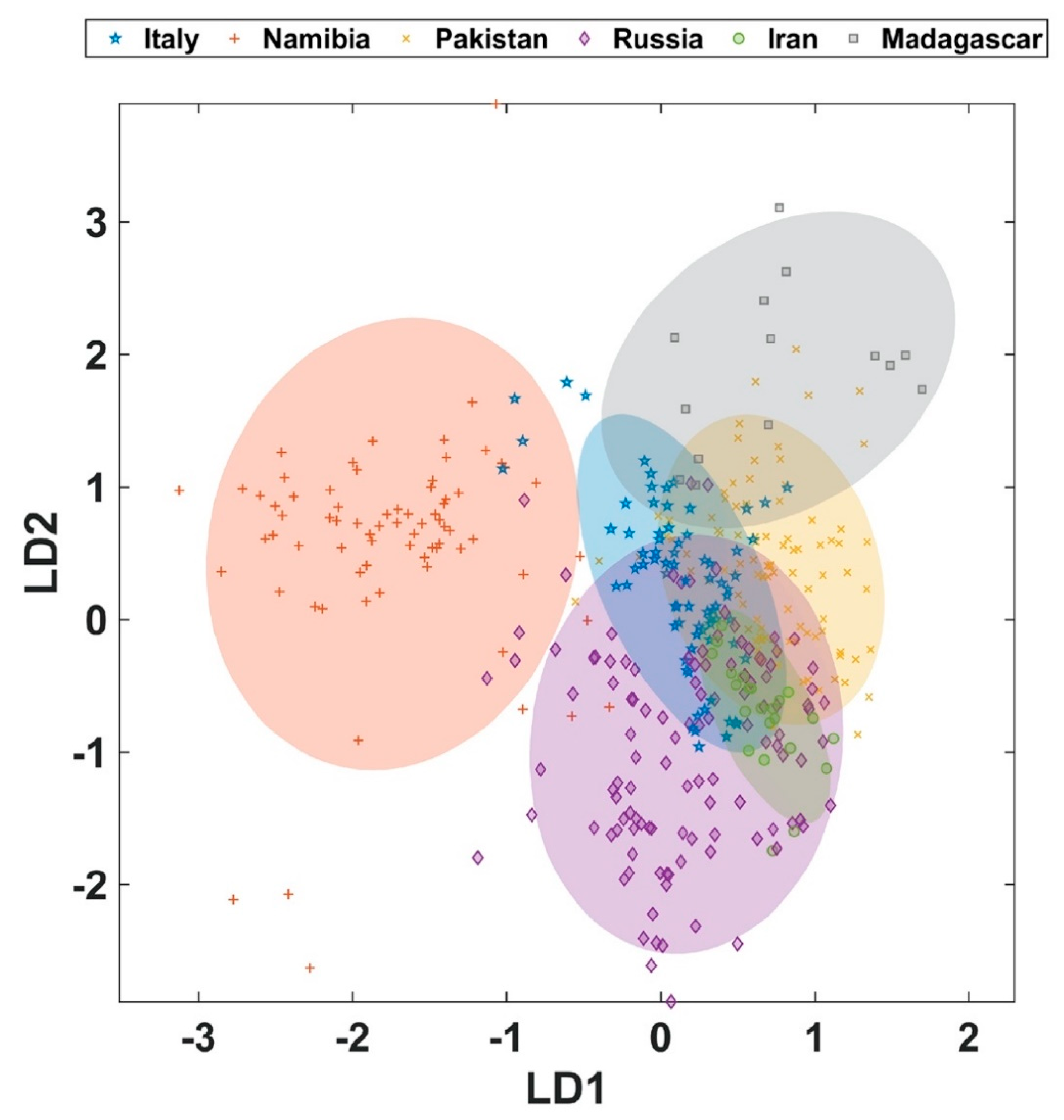
The model with all six origins shows that at least three origins can be predicted with a considerable high accuracy and precision (Figure 2, Table 1). In particular, demantoids from Namibia and Pakistan can be classified very well. Specimen from Madagascar can also be classified well, but the low prevalence leads to a higher degree of variability as evidenced by the larger standard deviation of the group accuracy resulting from MCCV. Although samples from Russian deposits can be predicted with accuracies around 80% some sample are mis-assigned to all other origins, except for Madagascar. This indicates a larger variability in the composition of these demantoids. Samples from Iran and Italy could also be assigned only with accuracies around 70%. However, in contrast to the wrongly classified samples from Russia the samples from Iran and Italy are mis-assigned to only two other origins. In particular demantoids from Italy exhibit a tendency to be predicted in a false-positive manner as Russian samples. This leads to the conclusion that a significant fraction of Italian demantoid samples shares a similar trace-element profile with the majority of the Russian samples. It should be mentioned that—although the prevalence index for five of the origins is met or even exceeded and only closely missed for the origin Iran—the smaller number of samples available for Iran and Madagascar adds to uncertainty. The question here is whether natural variability of these very difficult to come by samples is already adequately represented. Especially the narrow distribution of the profiles for Madagascar contributes to excellent classification properties for this particular deposit, which appears to source from an increased grossular content in the samples studied here. The small total number of data points also contributes to comparable large standard deviation of the class accuracy achieved during the 100-fold Monte Carlo cross-validation.
As already indicated above the number of samples has a critical influence on the model quality and should always be tested for using the prevalence threshold. In the above model the prevalence threshold for Iran was slightly missed as indicted by an asterisk in Table 2. This indicates that more samples will be needed to improve future models. However, at the same time this case represents an interesting test for what happens when locations with only small numbers of samples are included in modeling. While ideally all demantoid deposits in the world with all available specimens should be in a model this is not possible in reality, simply for sample availability, but also financial reasons associated with sample acquisition and analysis. As demantoids from Iran are present in the market we decided to include the available specimens into this model rather than to omit it and investigate the effects. While the model with six deposits does not allow satisfactory assignment of all samples in a single test the results from cross validation allow deepened insights into sample confusion. In fact, testing all classes in one model is only one of several possible testing strategies. A different strategy is to test one deposit in a pair-wise manner against all other deposits (i.e., testing location X vs. (combined others)). However, in this case the group consisting of all but one location displays a very high variability preventing improved results for the particular classification problem studied here (data not shown). It should be noted that it is difficult to delineate a generally applicable approach, as this will be determined by the properties of the population investigated. For the present case another possibility is inspired by the directed acyclic graph (DAG) trees [35]. Here, models are constructed for only two deposits at a time, but for all possible combination of deposits. By doing so the model can take optimal advantage of the differences between a particular pair of groups, which may lead to improved classification performance.
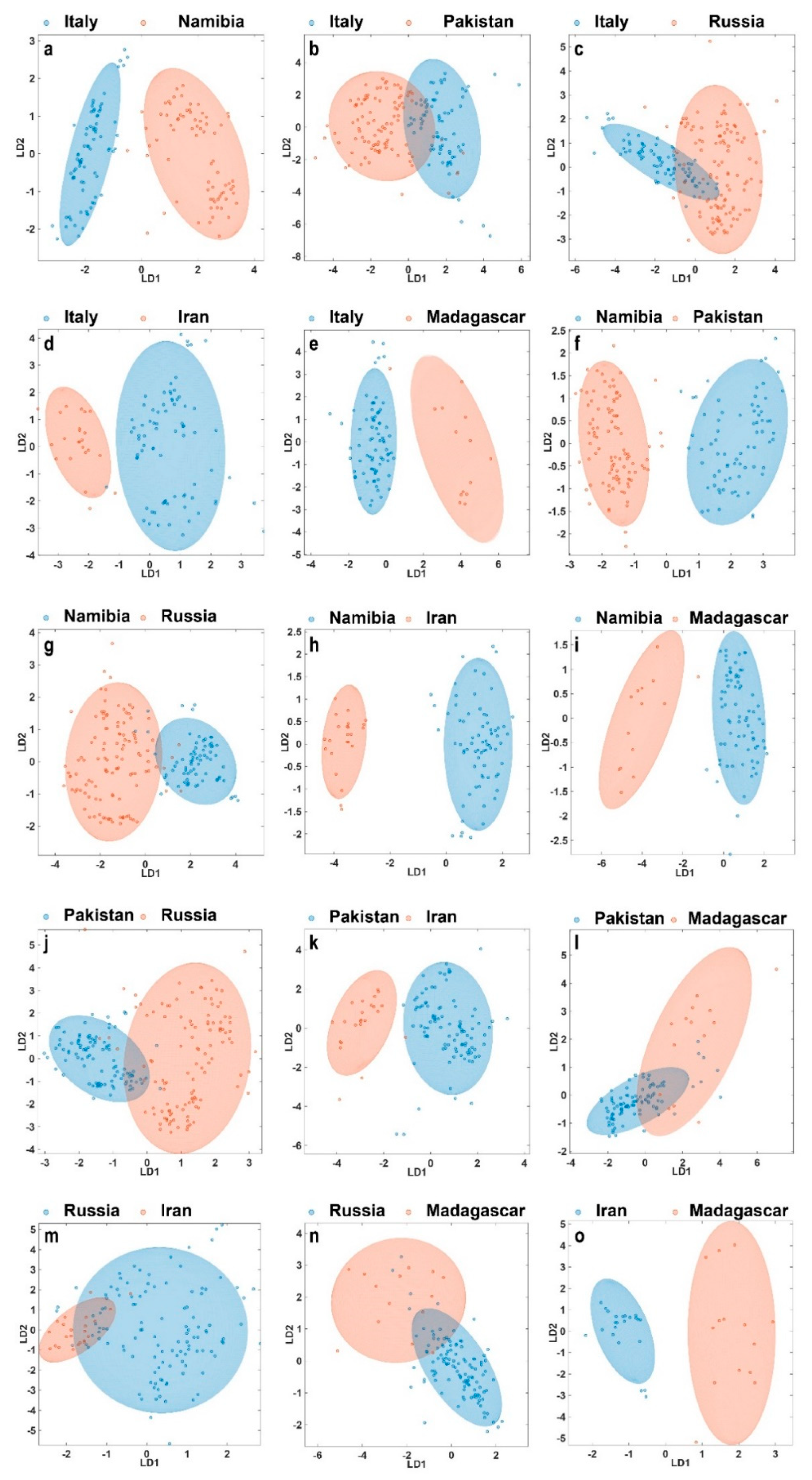
Hence, in order to better understand these pair-wise relationships we further established 15 models comparing only two selected origins (Figure 3). This is particularly interesting as now for each case a different set of variables can be used to describe the inter-group variance in an optimized way. The approach also has the potential that separations between two particular deposits can be much clearer than in the multi-origin model. However, caution is advised as an unknown sample subjected to classification with only two classes will be assigned to one of the two available choices—regardless if it is indeed a member of one of the two. For instance, if a garnet from Madagascar is investigated for class membership in a pair-wise model trained with samples from Italy and Pakistan, it will be assigned to one of these classes.
From a purely mathematical point of view it is non-sense to use something in a model for which it is not trained for. However, in real-life this is a realistic scenario when testing an unknown sample, especially if there is the suspicion of fraud. The unknown sample will be assigned to the class with the highest similarity. In case the sample does not belong to either of the groups tested for the Mahalanobis distance, which is a very useful metric for detecting multivariate outliers, for such a sample will likely be very large in comparison to samples that indeed belong to classes used for the training of the data set [36]. This is possible, for instance, through the QQ-plots (quantile-quantile) provided by the AI(OMICS)n package, where Mahalanobis distance of all samples used for model building and the sample under investigation is plotted versus their respective Euclidean distance at a 95% confidence level (α = 5%). In general, if an unknown sample is initially run in the multi-origin data set, one can obtain a first estimate of the samples’ country of origin. In a subsequent step this can be verified with the finer pair-wise models. In any case it is necessary to closely investigate the Mahalanobis distance for the sample in all models and to compare it with the typical confidence intervals obtained for true in-class samples.
Figure 3 clearly shows that even with only two depicted linear discriminators most origins can be clearly distinguished. In particular, Italy-Namibia, Italy-Iran, Italy-Madagascar, Namibia-Pakistan, Namibia-Iran, Namibia-Madagascar, Pakistan-Iran, and Iran-Madagascar can be separated essentially in full. For the remaining classification problems, it must not be forgotten that the graphs only represent 2D-projections of a multi-dimensional space and that the confusion matrix as well as additional metrics should be considered. Table 2 reveals that models for Madagascar typically exhibit a reasonable high accuracy which, however, varies considerably as a function of cross-validation. This can be explained to be a more frequent mis-assignment of only a few samples of the group, which due to the small group size accumulates to a large relative variation. Furthermore, Table 2 shows that the distinction of Italy vs. Russia and Russia vs. Iran works least as expressed by their low MCC of only 0.68 and 0.67, respectively. In both cases one group (Italy and Iran, respectively) shows a large number of mis-assigned samples. The first case is particularly interesting, as both groups are also present with comparable and larger sample numbers (Russia: 117, Italy: 78). While in this model Russian samples are mis-classified at a rate of only ~7% (8 out of 117), Italian samples are classified as being Russian demantoids at a rate of ~26% (20 out of 78). This means that the accuracy for both origins is different in this model, which has an impact on the interpretation of the results. Here, it is important to consider the testing hypothesis. This means that if the null hypothesis, H0, is Russia (we assume the sample is from Russia) there is a 93% chance the result is correct, and the gem is indeed from Russia. More than 9 out of 10 tests will deliver a correct result. However, in the case H0 is Italy (assuming the gem is from Italy) chances for the specimen being indeed an Italian demantoid are as low as 75% meaning one out of four tests will be mis-assigned. In such a case it is particularly important to critically evaluate all other models by attempting to rule out other solutions. Ultimately, there will always be a certain risk that a new sample is not well represented in the model. In such instances it is indicated to utilize additional approaches, such as analysis of inclusions (if present) to gain more confidence in the results obtained.
The confusion matrix for a representative model for pair-wise testing of the country of origin is shown in Table 2. Displayed are the model specific benchmark parameters accuracy (ACC), Matthews correlation coefficient (MCC), false classifications, correct classifications and the prevalence threshold (minimum calculated fraction/true fraction). Numbers in parenthesis are percent fractions for countries and correct and false classifications, respectively. n(total) denotes the number of total element profiles, n(class) the number of element profiles, and n(latent variables) the number of principal components used to achieve 95% explained variance. In addition, cumulative R2 and Q2 as well as the averaged group accuracy (mean ± standard deviation) from the 100-fold MCCV are shown to allow judgement of the model robustness. Diagonal elements in the confusion matrix represent the number (fraction) of correctly assigned cases. Models highlighted in red and blue denote perfectly (exclusively correct classifications) respectively almost perfectly preforming models.
A closer inspection of the VIP scores, i.e., the natural logarithms of elements, of the individual elements provides insights into their importance for a particular model (Table 3 and Table 4). Table 3 provides the detailed results for all models generated in this study, with VIP1 having the highest impact on a model and VIP6 having the lowest. Overall, it can be seen that Al and Cr appear to play a major role in the discriminant models, followed by Mg and Mn. However, it would be a wrong conclusion to assume that V and Ti could be omitted from the analysis. Despite these two elements playing a less important role in many of the generated models, they are essential components for the discrimination of Russia-Madagascar, Pakistan-Iran, Italy-Iran, and Iran-Madagascar. Moreover, valuable information about the importance of the elements for the within-class structure of the data is gained as the VIP method takes into account all dimensions of the generated model. Hence, for comprehensive analysis of the origin of a gem it is essential to record all six elements. In fact, it is the large range of concentrations found in natural gems which defines the origin of a specimen, when enough elements are combined. This can be visualized best by boxplots of the natural logarithms of the individual elements as a function of the country of origin. In the best cases, an origin can be selected (or excluded) by simply plotting the concentration profile into the boxplot chart (Figure 4).
4. Conclusions
We have successfully shown that the determination of country of origin is possible using a more quantitative approach than identification of inclusions, which is largely based on individual knowledge. By measuring minor and trace elements and applying modern chemometrics an excellent separation of five out of six countries of origin was achieved. The good separation with the complete dataset can even be improved when only a pair-wise comparison of two possible origins is used. This approach can be used when additional information, such as inclusions, can be used to rule out certain origins. Of course, the number of samples is essential for such studies and new samples will be added to the model as they become available. For the future it is planned to include even more elements into multivariate modelling. While it appears not rewarding to conduct large studies on elements that were shown to be not present in significant amounts in this and/or other studies, it seems promising to utilize major elements, such as Ca, Si, and Fe. As discussed for LA-ICP-MS proper calibration is difficult due to lacking standards and instrument limitations. This often prevents comparability of results obtained on different instruments. However, other technologies might be utilized in the future to obtain reproducible concentrations for these elements. Then, the data resulting from different technologies can be fused and evaluated together. This approach has already been successfully applied to technologies as different as NMR-spectroscopy and multi-isotope ratio mass-spectrometry [37].
Still, any such approach is only as good as the samples that are available. In our study the number of samples from Madagascar and Iran was rather limited with 5 and 8, respectively, so in order to improve the models more samples have to be obtained from those localities. New localities may be added as samples become available in significant numbers. Care has to be taken that selected specimens properly reflect the natural variability at these locations. Nevertheless, when applying such methods, the user has to be aware that likely not any sample population available will (a) ever represent all deposits in the world and (b) in significant numbers. Hence, interpretation shall always be carried out having this in mind. When testing samples for fraud, analytical results often provide hints that something is not as advertised. It is advisable to back up results with independent methods to get more evidence. Here, we have added one more tool to the analytical arsenal.
Supplementary Materials
The following are available online at https://www.mdpi.com/2075-163X/10/12/1046/s1, Table S1: Concentrations of Mg, Al, Ti, V, Cr, and Mn of all samples.
Author Contributions
Conceptualization, C.S. and S.S.; methodology, C.S. and S.S.; software, F.R. and S.S.; validation, S.G.B., F.R., S.S. and C.S.; formal analysis, S.G.B., F.R., S.S. and C.S.; investigation, S.G.B., F.R., S.S. and C.S.; resources, C.S. and S.S.; writing—original draft preparation, C.S., S.S. and S.G.B.; writing—review and editing, C.S., S.S., S.G.B. and F.R.; visualization, S.G.B.; project administration, C.S. and S.S.; funding acquisition, C.S. and S.S. All authors have read and agreed to the published version of the manuscript.
Funding
This research received no external funding.
Acknowledgments
The authors are grateful to Leopold Rößler (Austrian Gemmological Society), Gerhard Brandstetter, Ildar Latypov and Thomas Engeli for providing samples. Open Access Funding by the University of Linz.
Conflicts of Interest
The authors declare no conflict of interest.
References
- World Sapphire Market Update 2020 Lotus Gemology. Available online: https://lotusgemology.com/index.php/library/articles/459-world-sapphire-market-update-2020-lotus-gemology (accessed on 28 September 2020).
- Atkinson, D.; Kothavala, R.Z. Kashmir Sapphire. Gems. Gemol. 1983, 19, 64–76. [Google Scholar] [CrossRef]
- Palke, A.C.; Saeseaw, S.; Renfro, N.D.; Sun, Z.; McClure, S.F. Geographic Origin Determination of Blue Sapphire. Gems. Gemol. 2019, 55, 536–579. [Google Scholar] [CrossRef] [Green Version]
- Peretti, A.; Bieri, W.P.; Reusser, E.; Hametner, K.; Günther, D. Chemical Variations in Multicolored “Paraiba”-type Tourmalines from Brazil and Mozambique: Implications for Origin and Authenticity Determination. Contrib. Gemol. 2009, 9, 1–77. [Google Scholar]
- Kolesar, P.; Tvrdý, J. Zarenschätze; Rainer Bode: Haltern, Germany, 2006; p. 204. [Google Scholar]
- Burlakov, A.; Burlakov, E. Demantoid from Russia. InColor 2017, 36, 40–46. [Google Scholar]
- Reif, S. Green Dragon Mine Demantoid from Namibia. InColor 2017, 36, 48–52. [Google Scholar]
- Schwarzinger, C. Determination of demantoid garnet origin by chemical fingerprinting. Monats. Chem. 2019, 50, 907–912. [Google Scholar] [CrossRef] [Green Version]
- Adamo, I.; Bocchio, R.; Diella, V.; Pavese, A.; Vignola, P.; Prosperi, L.; Palanza, V. Demantoid from Val Malenco Italy: Review and Update. Gems. Gemol. 2009, 45, 280–287. [Google Scholar] [CrossRef] [Green Version]
- Pezzotta, F. Andradite from antetezambato, North Madagascar. Miner. Rec. 2010, 41, 209–229. [Google Scholar]
- Pezzotta, F.; Adamo, I.; Diella, V. Demantoid and Topazolite from Antetezambato, Northern Madagascar: Review and New Data. Gems. Gemol. 2011, 47, 2–14. [Google Scholar] [CrossRef]
- Palke, A.C.; Pardieu, V. Demantoid from Baluchistan Province in Pakistan. Gems. Gemol. 2014, 50, 302–303. [Google Scholar]
- Adamo, I.; Bocchio, R.; Diella, V.; Caucia, F.; Schmetzer, K. Demantoid from Balochistan, Pakistan: Gemmological and Mineralogical Characterization. J. Gemmol. 2015, 34, 428–433. [Google Scholar] [CrossRef]
- Hairapetian, V.; Pelckmans, H. Emerging Mineral Finds from Northern Iran. Rocks Miner. 2017, 6, 540–549. [Google Scholar] [CrossRef]
- Du Toit, G.; Mayerson, W.; Van Der Bogert, C.; Douman, M.; Befi, R.; Koivula, J.I.; Kiefert, L. Demantoid from Iran. Gems. Gemol. 2006, 42, 131. [Google Scholar]
- Schwarzinger, C.; Engeli, T. LA-ICP-MS spectrometry and its use in gemology. Ital. Gemol. Rev. 2019, 8, 50–52. [Google Scholar]
- Jochum, K.P.; Weis, U.; Stoll, B.; Kuzmin, D.; Yang, Q.; Raczek, I.; Jacob, D.E.; Stracke, A.; Birbaum, K.; Frick, D.A.; et al. Determination of reference values for NIST SRM 610–617 glasses following ISO guidelines. Geostand. Geoanal. Res. 2011, 35, 397–429. [Google Scholar] [CrossRef]
- Rüll, F.; Schwarzinger, S. AI(OMICS)n: A MatLab Based Expert System for Chemometrics and Data Fusion. 2020. Available online: https://gitlab.com/ai-omics/ai-omics/ (accessed on 20 October 2020).
- Kruskal, W.H.; Wallis, W.A. Use of ranks in one-criterion variance analysis. J. Am. Stat. Assoc. 1952, 47, 583–621. [Google Scholar] [CrossRef]
- Xu, Q.; Liang, Y.Z.; Du, Y.-P. Monto Carlo cross-validation for selecting a model and estimating the prediction error in multivariate calibration. J. Chemom. 2004, 18, 112–120. [Google Scholar] [CrossRef]
- Henningsson, M.; Sundbom, E.; Armelius, B.Å.; Erdberg, P. PLS model building: A multivariate approach to personality test data. Scand. J. Psychol. 2001, 42, 399–409. [Google Scholar] [CrossRef]
- Johansson, E.; Eriksson, L.; Sandberg, M.; Wold, S. QSAR Model Validation. In Molecular Modeling and Prediction of Bioactivity; Springer: Boston, MA, USA, 2000. [Google Scholar] [CrossRef]
- Wold, S.; Sjöström, M.; Eriksson, L. PLS-regression: A basic tool of chemometrics. Chemom. Intell. Lab. Syst. 2001, 58, 109–130. [Google Scholar] [CrossRef]
- Matthews, B.W. Comparison of the predicted and observed secondary structure of T4 phage lysozyme. Biochim. Biophys. Acta 1975, 405, 442–451. [Google Scholar] [CrossRef]
- Baldi, P.; Brunak, S.; Chauvin, Y.; Andersen, C.A.; Nielsen, H. Assessing the accuracy of prediction algorithms for classification: An overview. Bioinformatics 2000, 16, 412–424. [Google Scholar] [CrossRef] [PubMed] [Green Version]
- Balayla, J. Prevalence threshold (ϕe) and the geometry of screening curves. PLoS ONE 2020, 15, e0240215. [Google Scholar] [CrossRef] [PubMed]
- R Core Team. R: A Language and Environment for Statistical Computing; R Foundation for Statistical Computing: Vienna, Austria, 2020; Available online: https://www.R-project.org/ (accessed on 20 October 2020).
- Huelin, S.R.; Longerich, H.P.; Wilton, D.H.; Fryer, B.J. The determination of trace elements in Fe–Mn oxide coatings on pebbles using LA-ICP-MS. J. Geochem. Expl. 2006, 91, 110–124. [Google Scholar] [CrossRef]
- van den Berg, R.A.; Hoefsloot, H.C.; Westerhuis, J.A.; Smilde, A.K.; van der Werf, M.J. Centering, scaling, and transformations: Improving the biological information content of metabolomics data. BMC Genom. 2006, 7, 142. [Google Scholar] [CrossRef] [PubMed] [Green Version]
- Kolb, P.; Bindereif, S.G.; Rüll, F.; Schwarzinger, S. unpublished data, to be published elsewhere.
- Mahalanobis, P.C. On the Generalized Distance in Statistics. Proc. Natl. Inst. Sci. India 1936, 2, 49–55. [Google Scholar]
- Moawed, S.A.; Osman, M.M. The robustness of binary logistic regression and linear discriminant analysis for the classification and differentiation between dairy cows and buffaloes. Int. J. Stat. Appl. 2017, 7, 304. [Google Scholar] [CrossRef]
- Barragués, J.I.; Morais, A.; Guisasola, J. (Eds.) Probability and Statistics: A didactic Introduction; CRC Press: Boca Raton, FL, USA, 2014. [Google Scholar]
- Hotelling, H. The generalization of Student’s ratio. Ann. Math. Statist. 1931, 2, 360–378. [Google Scholar] [CrossRef]
- Platt, J.C.; Cristianini, N.; Shawe-Taylor, J. Large Margin DAGs for Multiclass Classification. Adv. Neural Inf. Process. Syst. 2000, 12, 547. [Google Scholar]
- Ghorbani, H. Mahlanobis distance and its application for detecting multivariate outliers. Facta Univ. (NIS) Ser. Math. Inform. 2019, 34, 583. [Google Scholar] [CrossRef]
- Bindereif, S.G.; Brauer, F.; Schubert, J.-M.; Schwarzinger, S.; Gebauer, G. Complementary use of 1H NMR and multi-element IRMS in association with chemometrics enables effective origin analysis of cocoa beans (Theobroma cacao L.). Food Chem. 2019, 299, 125105. [Google Scholar] [CrossRef]
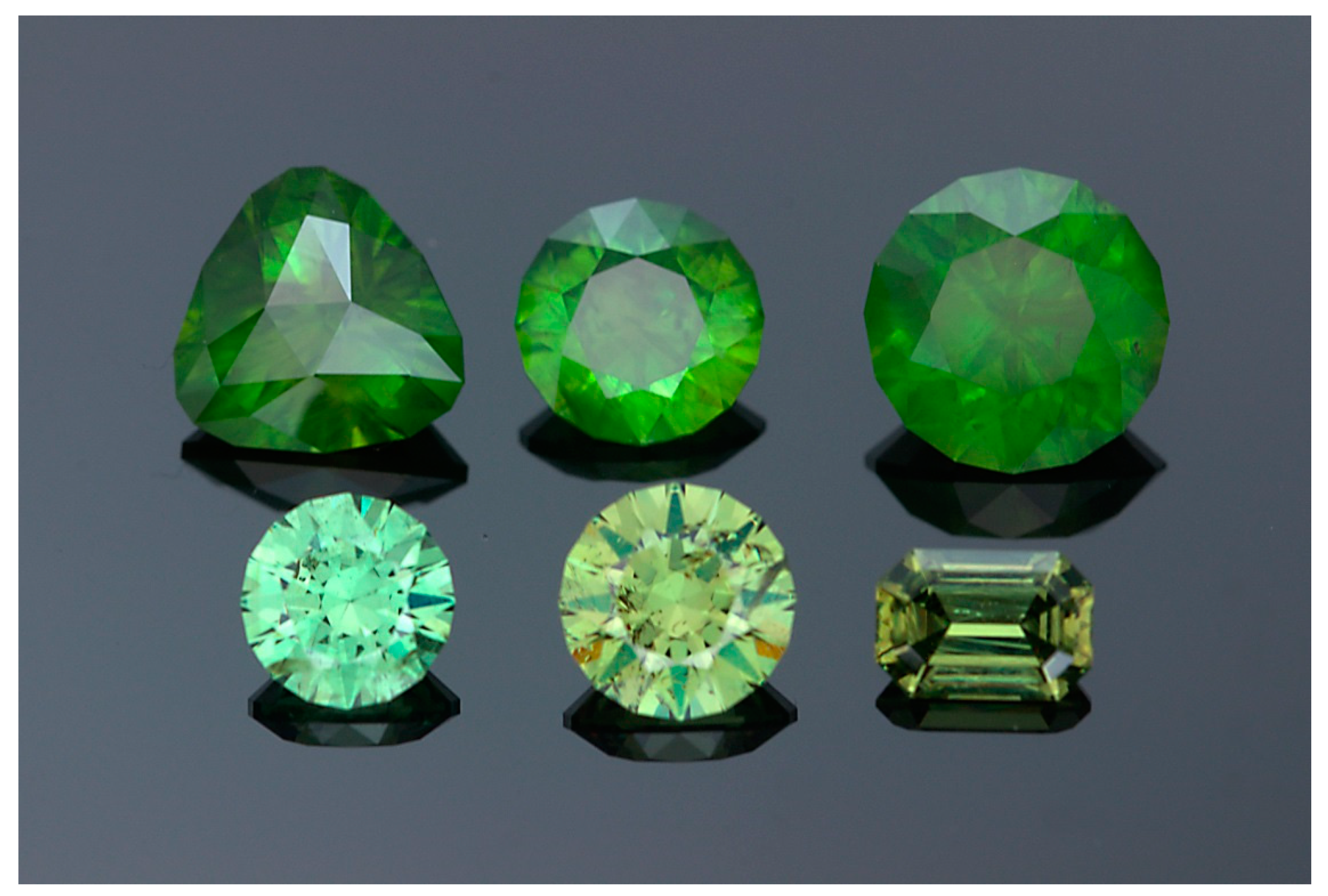
Figure 1.
Demantoid gemstones (0.75–3.23 ct) from Russia (top row) and Namibia (bottom row) represent the majority of today’s market.
Figure 1.
Demantoid gemstones (0.75–3.23 ct) from Russia (top row) and Namibia (bottom row) represent the majority of today’s market.

Figure 2.
PCA-LDA score plot with all classes including the log-transformed concentrations of the six relevant elements Mg, Al, Ti, V, Cr and Mn. Each dot represents a single element profile from an individual measurement after MCCV. Axis shown represent the first two linear discriminants. Ellipses confer to the 95% confidence interval according to Hotellings T2, which is the multivariate analog to the t-test [34]. Note that graphics represent a projection from 6-dimensional space, i.e., overlap in this projection does not necessarily mean samples cannot be separated (cf. confusion matrix in Table 1).

Figure 3.
Representative PCA-LDAs for the pair-wise models (a) Italy-Namibia; (b) Italy-Pakistan; (c) Italy-Russia; (d) Italy-Iran; (e) Italy-Madagascar; (f) Namibia-Pakistan; (g) Namibia-Russia, (h) Namibia-Iran; (i) Namibia-Madagascar, (j) Pakistan-Russia, (k) Pakistan-Iran, (l) Pakistan-Madagascar, (m) Russia-Iran, (n) Russia-Madagascar, (o) Iran-Madagascar. Each dot represents a single element profile from an individual measurement after MC cross-validation. Axis shown represent the first two linear discriminants. Ellipses confer to the 95% confidence interval according to Hotellings T2.

Figure 4.
Boxplot showing the natural logarithm of all measured element concentrations. Samples are grouped and colored by origin. The graph displays the median, the first quartile, the third quartile as well as the maximum and minimum of each group. Outliers are represented as black dots.
Figure 4.
Boxplot showing the natural logarithm of all measured element concentrations. Samples are grouped and colored by origin. The graph displays the median, the first quartile, the third quartile as well as the maximum and minimum of each group. Outliers are represented as black dots.


Table 1.
Confusion matrix showing prediction accuracy of the method (for details refer to the text).
Table 1.
Confusion matrix showing prediction accuracy of the method (for details refer to the text).
| Model | ACC = 0.84 | MCC = 0.78 | R2cum = 1 | Q2cum = 0.85 | |||
|---|---|---|---|---|---|---|---|
| All Origins | |||||||
| n(total) = 403 | True Namibia | True Pakistan | True Madagascar | True Russia | True Iran | True Italy | prevalence threshold (calc/observed) |
| Predicted Namibia | 68 (93.2%) | 0 | 0 | 5 (4.3%) | 0 | 0 | 0.12/0.18 |
| Predicted Pakistan | 0 | 91 (92.9%) | 1 (7.1%) | 7 (6.0%) | 0 | 7 (9.0%) | 0.12/0.18 |
| Predicted Madagascar | 0 | 0 | 13 (92.9%) | 0 | 0 | 0 | 0.03/0.03 |
| Predicted Russia | 2 (2.7%) | 1 (1.0%) | 0 | 96 (82.1%) | 3 (13.0%) | 18 (23.1%) | 0.24/0.29 |
| Predicted Iran | 0 | 1 (1.0%) | 0 | 3 (2.6%) | 17 (73.9%) | 0 | 0.10/0.06 * |
| Predicted Italy | 3 (4.1%) | 5 (5.1%) | 0 | 6 (5.1%) | 3 (13.0%) | 53 (67.9%) | 0.22/0.19 |
| n(class) | 73 | 98 | 14 | 117 | 23 | 78 | |
| false classifications (n (%)) | 65 (16.1%) | ||||||
| correct classifications (n (%)) | 338 (83.9 %) | ||||||
| n(latent variables) | 6 | ||||||
| Averaged Group Accuracy from MC cross validation | 0.92 ± 0.10 | 0.91 ± 0.10 | 0.94 ± 0.15 | 0.81 ± 0.12 | 0.72 ± 0.31 | 0.68 ± 0.18 | |
*: Prevalence threshold missed for location Iran—see text for details. Model performance (correctly assigned) indicated by background color: >90%: green; >80 %: blue; >70 % yellow; rest: red.
Table 2.
Confusion matrix for a representative model for pair-wise testing of the country of origin (15 individual models).
Table 2.
Confusion matrix for a representative model for pair-wise testing of the country of origin (15 individual models).
 |
Models allowing invariably correct assignments are highlighted in red; models performing better than 99% and a standard deviation <5% are shown in blue.
Table 3.
Listing of the most important variables for each model ranked by their VIP-score.
| Model | Type of Deposit | VIP1 | VIP2 | VIP3 | VIP4 | VIP5 | VIP6 |
|---|---|---|---|---|---|---|---|
| All origins | ln(Mg) | ln(Cr) | ln(Ti) | ln(Al) | ln(Mn) | ln(V) | |
| Italy-Namibia | asbestos vs. skarn | ln(Al) | ln(Cr) | ln(Mn) | ln(Ti) | ln(Mg) | ln(V) |
| Italy-Pakistan | asbestos vs. asbestos | ln(Mn) | ln(Mg) | ln(Al) | ln(Cr) | ln(Ti) | ln(V) |
| Italy-Russia | asbestos vs. asbestos | ln(Mg) | ln(Al) | ln(V) | ln(Ti) | ln(Cr) | ln(Mn) |
| Italy-Iran | asbestos vs. asbestos | ln(Al) | ln(Ti) | ln(Cr) | ln(Mn) | ln(Mg) | ln(V) |
| Italy-Madagascar | asbestos vs. skarn | ln(Cr) | ln(Al) | ln(Mg) | ln(V) | ln(Ti) | ln(Mn) |
| Namibia-Pakistan | asbestos vs. skarn | ln(Al) | ln(Cr) | ln(Mg) | ln(Mn) | ln(V) | ln(Ti) |
| Namibia-Russia | asbestos vs. skarn | ln(Al) | ln(Mn) | ln(V) | ln(Ti) | ln(Cr) | ln(Mg) |
| Namibia-Iran | asbestos vs. skarn | ln(Mn) | ln(Mg) | ln(Cr) | ln(Ti) | ln(Al) | ln(V) |
| Namibia-Madagascar | skarn vs. skarn | ln(Cr) | ln(Mg) | ln(Mn) | ln(Al) | ln(Ti) | ln(V) |
| Pakistan-Russia | asbestos vs. asbestos | ln(Mg) | ln(Al) | ln(Cr) | ln(Ti) | ln(V) | ln(Mn) |
| Pakistan-Iran | asbestos vs. asbestos | ln(V) | ln(Cr) | ln(Al) | ln(Ti) | ln(Mg) | ln(Mn) |
| Pakistan-Madagascar | asbestos vs. skarn | ln(Cr) | ln(Mn) | ln(Mg) | ln(Al) | ln(Ti) | ln(V) |
| Russia-Iran | asbestos vs. asbestos | ln(Cr) | ln(Al) | ln(Mg) | ln(Mn) | ln(Ti) | ln(V) |
| Russia-Madagascar | asbestos vs. skarn | ln(V) | ln(Cr) | ln(Al) | ln(Mg) | ln(Ti) | ln(Mn) |
| Iran-Madagascar | asbestos vs. skarn | ln(Cr) | ln(V) | ln(Al) | ln(Ti) | ln(Mg) | ln(Mn) |
Table 4.
Scores of the individual elements as a function of their VIP-rank. Although it appears that Ti and V are overall of less importance Table 3 clearly indicates their important role for particular models.
Table 4.
Scores of the individual elements as a function of their VIP-rank. Although it appears that Ti and V are overall of less importance Table 3 clearly indicates their important role for particular models.
| Rank VIP | Al | Cr | Mg | Mn | Ti | V |
|---|---|---|---|---|---|---|
| 1 | 4 | 5 | 3 | 2 | 0 | 2 |
| 2 | 4 | 5 | 3 | 2 | 1 | 1 |
| 3 | 4 | 3 | 4 | 2 | 1 | 2 |
| 4 | 3 | 1 | 1 | 3 | 7 | 1 |
| 5 | 1 | 2 | 4 | 1 | 6 | 2 |
| 6 | 0 | 0 | 1 | 6 | 1 | 8 |
Publisher’s Note: MDPI stays neutral with regard to jurisdictional claims in published maps and institutional affiliations. |
© 2020 by the authors. Licensee MDPI, Basel, Switzerland. This article is an open access article distributed under the terms and conditions of the Creative Commons Attribution (CC BY) license (http://creativecommons.org/licenses/by/4.0/).
Share and Cite
MDPI and ACS Style
Bindereif, S.G.; Rüll, F.; Schwarzinger, S.; Schwarzinger, C. Chemometric Modeling of Trace Element Data for Origin Determination of Demantoid Garnets. Minerals 2020, 10, 1046. https://doi.org/10.3390/min10121046
AMA Style
Bindereif SG, Rüll F, Schwarzinger S, Schwarzinger C. Chemometric Modeling of Trace Element Data for Origin Determination of Demantoid Garnets. Minerals. 2020; 10(12):1046. https://doi.org/10.3390/min10121046
Chicago/Turabian StyleBindereif, Stefan G., Felix Rüll, Stephan Schwarzinger, and Clemens Schwarzinger. 2020. "Chemometric Modeling of Trace Element Data for Origin Determination of Demantoid Garnets" Minerals 10, no. 12: 1046. https://doi.org/10.3390/min10121046
Note that from the first issue of 2016, this journal uses article numbers instead of page numbers. See further details here.