The Water Footprint of the United States


1
Department of Civil and Environmental Engineering, University of Illinois at Urbana Champaign, Champaign IL 61801, USA
2
Department of Civil and Environmental Engineering, Virginia Tech, Blacksburg, VA 24061, USA
*
Author to whom correspondence should be addressed.
†
These authors contributed equally to this work.
Water 2020, 12(11), 3286; https://doi.org/10.3390/w12113286
Submission received: 1 October 2020
/
Revised: 13 November 2020
/
Accepted: 18 November 2020
/
Published: 23 November 2020
(This article belongs to the Special Issue In Memory of Prof. Arjen Y. Hoekstra)
Abstract
:This paper commemorates the influence of Arjen Y. Hoekstra on water footprint research of the United States. It is part of the Special Issue “In Memory of Prof. Arjen Y. Hoekstra”. Arjen Y. Hoekstra both inspired and enabled a community of scholars to work on understanding the water footprint of the United States. He did this by comprehensively establishing the terminology and methodology that serves as the foundation for water footprint research. His work on the water footprint of humanity at the global scale highlighted the key role of a few nations in the global water footprint of production, consumption, and virtual water trade. This research inspired water scholars to focus on the United States by highlighting its key role amongst world nations. Importantly, he enabled the research of many others by making water footprint estimates freely available. We review the state of the literature on water footprints of the United States, including its water footprint of production, consumption, and virtual water flows. Additionally, we highlight metrics that have been developed to assess the vulnerability, resiliency, sustainability, and equity of sub-national water footprints and domestic virtual water flows. We highlight opportunities for future research.
1. Introduction
Arjen Y. Hoekstra (AYH) pioneered the field of water footprinting [1]. He developed the core terminology that the water footprint community continues to use and build from [2]. Importantly, AYH provided freely available access to water footprint data and model estimates, enabling the community of water footprint researchers to build from his foundation. AYH’s research comprehensively evaluated the water footprint of humanity [3]. His research highlighted the key role of certain nations—including the United States—to the global water footprint of humanity. In this way, his work inspired a community of scholars to delve deeper into the water footprint of the United States. This paper commemorates the influence of AYH to the community of scholars working on the water footprint of the United States and is part of a collection of papers in the Special Issue “In Memory of Prof. Arjen Y. Hoekstra”. The goal of this paper is not to serve as a comprehensive or critical review of research on the water footprint of the United States, but, rather, to pay tribute to Arjen Y. Hoekstra on the anniversary of his untimely passing.
The United States is a major economic producer, consumer, and trade power. The economy and supply chains of the US rely on water resources [4]. The US is a key nation in the global virtual water trade network [5], contributing the most virtual water to global trade [3]. International virtual water trade with the US is enabled by a host of interconnected infrastructure [6]. The spatial distribution of water security within the US influences where water-intensive goods are produced. Water hazards and risk further shape production and disrupt supply chains [7]. In turn, supply chains can shape water resources and influence their sustainability [8]. Water stress varies spatially and across economic sectors in the US [7]. Water footprints identify counties in the US where human water use exceeds renewable water supplies [9,10,11].
Water withdrawals in the United States in 2015 was estimated to be about 445 billion m3 [12]. Information on national and county-scale water use is provided by the US Geological Survey, which is a vital source of water withdrawal data that underpins many studies of water use in the US economy [13]. Freshwater withdrawals were 388 m3, or 87 percent of total withdrawals (saline-water withdrawals comprise the remaining 13 percent) [12]. National water use has been declining over the past several decades, largely due to productivity gains in the economy [14]. Long-term structural changes in the US economy (e.g., increasing service sector) and productivity improvements in electricity generation and shifts to producing less water-intensive products has driven this reduction at the national scale [14,15]. The trend in water use varies by a source of water, with declines in surface-water withdrawals and increases in fresh groundwater withdrawals in the most recent national data [12]. Controls on water use are not uniform across the nation. Water use in the Northeast and Northwest is driven by social variables, whereas climate primarily influences water use in the Southwest [16].
AYH introduced water footprints to quantify the link between human consumption and the appropriation of freshwater [17]. In this way, he introduced supply-chain thinking to the field of water resources management [18]. Following the definitions put forth by AYH, most water footprint studies calculate consumptive use of water resources per unit product produced (see Table 1) [2,3], or the water use that is no longer immediately available in the local area for further use (e.g., crop evapotranspiration). However, some studies, particularly those that consider the water footprint of energy, also consider the withdrawal use of water [19], or the volume abstracted from a water source. Most water footprint assessments have historically focused on agriculture, since it accounts for the vast majority of consumptive water use, meaning that this water will no longer be usable in the location from which it was withdrawn. This differs from withdrawal uses of water, which include return flows that can be utilized again in the location of use. Studies that employ the water footprint concept but replace water consumption with withdrawals tend to emphasize the importance of water use for thermoelectric power generation in the United States, while consumptive water footprints emphasize agriculture at the expense of the energy sector (since most energy water use is non-consumptive). Together, the energy and agriculture sectors constitute over four-fifths of blue water consumption and withdrawals [4,12].
The source of the water is important to determine when assessing water footprints. AYH made significant strides in partitioning water footprints into different types of water: “green”, “blue”, and “grey” [2,3]. “Green” water is the soil moisture derived from precipitation, while “blue” water is water from a source, such as a reservoir, river, lake, or aquifer [2]. “Grey” water refers to the water required to dilute pollutants to a regulatory threshold [2]. Water footprint research in the United States has continued to resolve domestic water footprints with increasing refinement by type of water. Several studies in the US further resolve water sources by unsustainable surface and subsurface contributions [20,21]. Increased attention has also been devoted to how specific water bodies contribute to domestic and international supply chains [22,23]. The remainder of this paper provides an overview of research that has increasingly refined our understanding of the spatial, temporal, and commodity resolution of water footprints and virtual water transfers within the United States. Note that the term virtual water transfers are used instead of virtual water trade to indicate intra-national virtual water flows rather than trade between nations. The development of metrics to capture the dependencies, resilience, vulnerability, sustainability, and equity of virtual water flows is surveyed. This paper concludes with suggestions for future work.
2. The Water Footprint of Production
Water is a critical input in the production of commodities, goods, and services in the US. The water footprint metric developed by Arjen Y. Hoekstra [18] provided a new tool to clearly and consistently quantify the role of water within the economy. The water footprint of a product is the total volume of freshwater (blue, green, and grey) directly and indirectly consumed in the production of a product across its entire supply chain [18]. The water footprint of a product can be normalized against some production measure (e.g., yield, mass, value, kilo-calories, etc.) so that water consumption can be compared relative to some metric of interest. This normalized water footprint of a product is sometimes called the product’s virtual water content (VWC), although AYH preferred to use the term “water footprint per unit of production” [18].
From this water footprint concept, AYH developed a rigorous methodology and water footprint data that has been utilized by researchers around the world and serves as the foundation for most of the US water footprint and virtual water transfer studies surveyed here. While early water footprint estimates in the United States predominately focused on agricultural products, recent years have seen advances in other sectors, particularly the energy sector. Studies are increasingly moving to more spatially refined and commodity-specific estimates of production water footprints. Moreover, the relative abundance of publicly-available water and economic data in the US has enabled US water footprint studies to build on AYH’s earlier research by delineating not only blue, green, and grey water footprints but also denoting whether the water was from surface or groundwater sources, as well as the sustainability of the water footprint.
Agriculture has the largest total water footprint of any sector in the US. Between 74–93% (94–170 km3) of all blue water consumed in the US is for irrigated agriculture and livestock production [4,24]. Of this, 44% comes from streams, rivers, and lakes, while the remaining 56% is from groundwater. The High Plains, Mississippi Embayment, and Central Valley aquifers supply the vast majority of the groundwater used for crop irrigation in the US [4,23]. Nearly 80% of all agricultural blue water footprints occur west of the 97th meridian west, which divides the humid eastern US from the arid Western plains [4].
The blue water footprint of food production is strongly linked to agricultural production locations [24], irrigation technology and management [25,26], and eventual food produced [27]. Corn grain and silage, hay and haylage, rice, wheat, soybeans, cotton, and almonds constitute 47% of the surface and 75% of the groundwater footprint in the US [4]. Crops like almonds [28] and livestock feed [20] have been highlighted for their relatively large blue water footprint and their propensity for being produced in water-scarce areas within the US. While the livestock industry is often highlighted for the large burden it places on the nation’s water resources, recent work by AYH shows that the US livestock industry has seen significant water productivity gains (between two- to four-fold) over the last six decades [29].
In recent years, AYH has argued that it is important to recognize the role of green water in production and for the need to properly manage this resource [30,31]. There is a competition for limited green water resources between the environment and society, since we use green water to produce food, fiber, animal feed, timber, and bioenergy crops. AYH argued that many areas, including some areas within the US, face green water scarcity. Green water scarcity is a metric that considers green water footprints relative to the abundance of green water and environmental flow requirements to support biodiversity [31]. In the US, green water constitutes over 86% (602 km3) of the total water footprint of agriculture and nearly 83% of the US economy’s total consumption of water [4]. Given the importance of green water to the US economy, Xu et al. [32] assessed the green water resources available for crop production in the US for food, feed, and biofuels and the impact these demands have on natural ecosystems (e.g., forest, grassland, environmental flows). Agricultural production uses less than one-third of the available green water resources across the US. However, at the county level, there are instances of green water scarcity, including the Corn Belt, which covers the states of Iowa, Illinois, Minnesota, Nebraska, and South Dakota [32].
Water footprint studies of agriculture delineate between blue and green water sources, yet these two sources of water are interlinked. For example, preseason soil moisture, which is primarily from precipitation, can dramatically reduce the need for crop irrigation throughout the growing season. Preseason soil moisture can reduce blue water requirements in the Corn Belt by 96% (1.9 versus 45.5 billion m3/year) [33]. During soil moisture drought events, producers will often increase irrigation (i.e., blue water) to make up for a green water deficit. For instance, irrigators in California’s Central Valley used groundwater to buffer against green and surface water deficits during the 2012–2015 drought [34]. A complex blend of market forces, policy, and regulation has led this water-scarce region to produce more water-intensive but higher-value crops over the last few decades [28,34,35]. Water-stressed agricultural regions of the US, such as California, could achieve significant water savings (56% water savings) by growing crops better suited to the green water availability of the area [36].
The water footprint of agriculture in the US constitutes more than food, fiber, and feed. The 2007 Energy Independence and Security Act (EISA) expanded biofuel blending requirements, strengthening the linkage between the energy and agriculture sectors, as well as the water inputs foundational to both sectors [37,38]. The primary feedstocks for US biofuels are corn (ethanol) and soybeans (biodiesel), which have seen an expansion in production since 2007. The amount of blue and green water required to irrigate biofuel feedstock varies spatially, temporally, and by feedstock crop. Groundwater is the dominant blue water source for feedstock irrigation in most of the US [39]. Significant spatial variability of the blue, green, and grey water footprints of biofuel exist at the county-level [39]. Vehicles consume approximately 118 L of water per km (lwpkm) when using irrigated corn-based ethanol from Nebraska, but only 54 L of water if fueled by Iowa irrigated corn-based ethanol [37]. Similarly, irrigated sorghum-based ethanol from Texas is more water-intensive than if it is grown in Nebraska [37]. Scown et al. [40] finds that some biofuels can have a blue water footprint more than two orders of magnitude larger than traditional gasoline-based transportation fuels.
The blue water footprint of traditional fuels, such as oil and natural gas, is increasing within the US [41]. At the national level, the blue water footprint of this sector is not a significant water user. Its annual blue water footprint was 1.82 × 10⁸ m3 between 2012–2014, or roughly 0.14% of the US economy’s blue water footprint [4,42]. However, water used in oil and natural gas production, including water used for hydraulic fracturing and flowback-produced water, can constitute a significant portion of local water budgets. The water footprint of oil production in the Bakken Play, which stretches across North Dakota, Montana, and Canada, has increased six-fold from 2005–2014 and is expected to increase another ten-fold from 2014–2050 due to larger water use per well and the addition of 60,000 producing wells throughout the region [43]. Between 2011–2016, the blue water footprint of hydraulic fracturing and wastewater production per well has increased 770% across major shale gas and oil production regions in the US [41].
The US energy system accounts for roughly 10% of the national blue water footprint and about 40% of total water withdrawals [19]. Water withdrawals are driven by once-through cooling systems of thermoelectric plants (approximately 70% of withdrawals) [19]. However, most of the water withdrawals of once-through thermoelectric power plants are returned to the water source, albeit at a higher temperature. Chini et al. [44] uses an adapted version of AYH’s grey water footprint to estimate the water needed to bring the heated return flow from each thermoelectric power plant in the contiguous US back to an allowable limit.
Energy from hydropower, ethanol, and conventional oil have the largest blue water footprint within the US energy sector [19,45]. Since hydropower typically uses instream flows to generate electricity, water consumption associated with this energy source has not been well-documented. AYH first calculated the magnitude of the blue water footprint of hydropower by estimating reservoir evaporation associated with the hydropower facilities [46]. Grubert [47] built on the global study by AYH, using detailed, facility-specific data within the US to estimate the blue water footprint for nearly 2200 hydropower facilities. Water footprint assessments are highly sensitive to the methodology used to calculate the water footprint of hydropower and the inclusion of hydropower in the water footprint of energy production studies can skew results due to relatively large volumes of water consumption attributed to this form of energy generation [47,48].
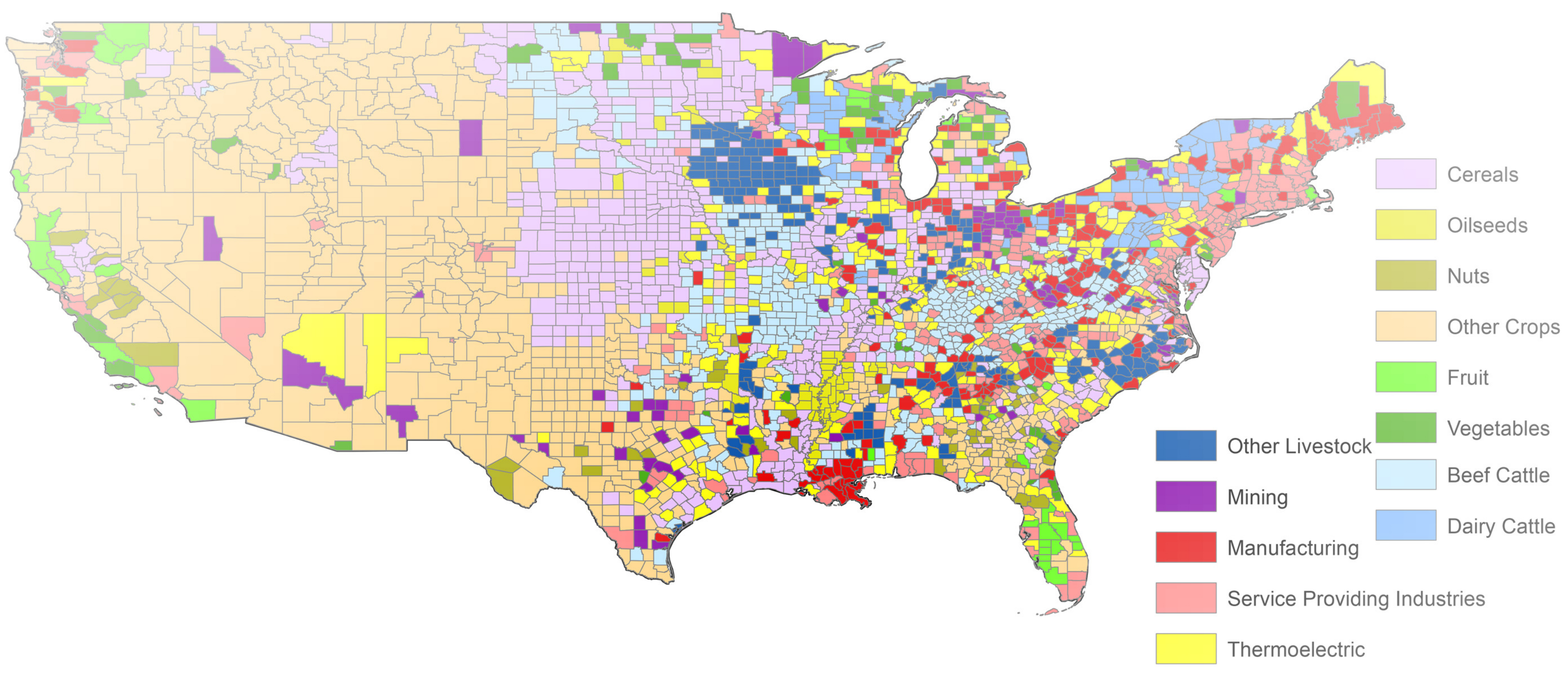
In one of AYH’s most cited and acclaimed papers [3], he shifted the focus of water footprint assessments from strictly the agriculture and energy sectors to more broadly identify all the ways society utilizes water around the world. Years later, we worked with AYH and his close colleague and former student, Mesfin Mekonnen, on a similar study detailing the blue and green water footprint of over 500 US products and industries [4] (see Figure 1). This remains one of the most detailed national water footprint assessments to date, largely due to the abundance of US-based data and studies available to us to build upon. Chief among these data is the United States Geological Survey (USGS) National Water Census [12]. Industrial, commercial, mining, and institutional water footprints are highly variable and difficult to estimate with empirical or processed-based models, which is why nearly every US water footprint study depends on the USGS’s National Water Census [4,24,49,50,51]. A handful of city-level or regional studies collect local data on industrial and other municipal water uses directly from water utilities, municipalities, or state agencies [22,52]. Water footprint assessments have enabled researchers to employ multi-region input-output (MRIO) models to better understand how water is used throughout the US economy [4,22,51,53,54,55].
3. Sub-National Virtual Water Flows
Arjen Y. Hoekstra defined and calculated virtual water trade between nations using the water footprint of a unit product and international trade data [3]. Following AYH’s approach, sub-national virtual water flow estimation requires both product water footprint and commodity flow information. The main distinction is that commodity trade data is between countries while commodity flow data is more generic and captures the movement of goods between other political units. Sub-national virtual water flows are calculated by multiplying the flow amount by the unit commodity water footprint in the source location as follows:
where is the virtual water flow [volume], is the water footprint per unit commodity [volume/mass], and F is the commodity flow [mass]. The variables are indexed by subscripts o for origin, d for destination, c for commodity, and y for year. Note that the water footprint could alternatively be provided in units of water volume per dollar [$] to pair with dollar value flow data.
One of the major reasons for virtual water flow studies within the United States is the availability of sub-national flow information. For example, data on sub-national commodity flows is available within the United States from the Commodity Flow Survey (CFS) and the Freight Analysis Framework (FAF). Many studies pair AYH’s product water footprint data with CFS/FAF data to quantify sub-national virtual water flows [56], including flows from specific locations within the US to international destinations [23], since FAF includes international destinations. Similarly, there are sub-national data on the movement of electricity throughout the electric grid of the US, enabling studies to determine the virtual flows of water associated with electricity [57]. Thus, the availability of sub-national commodity flow information has enabled much research on virtual water flows within the US. These studies have typically focused on agri-food and energy supply chains, with increasing spatial, temporal, and water source refinement.
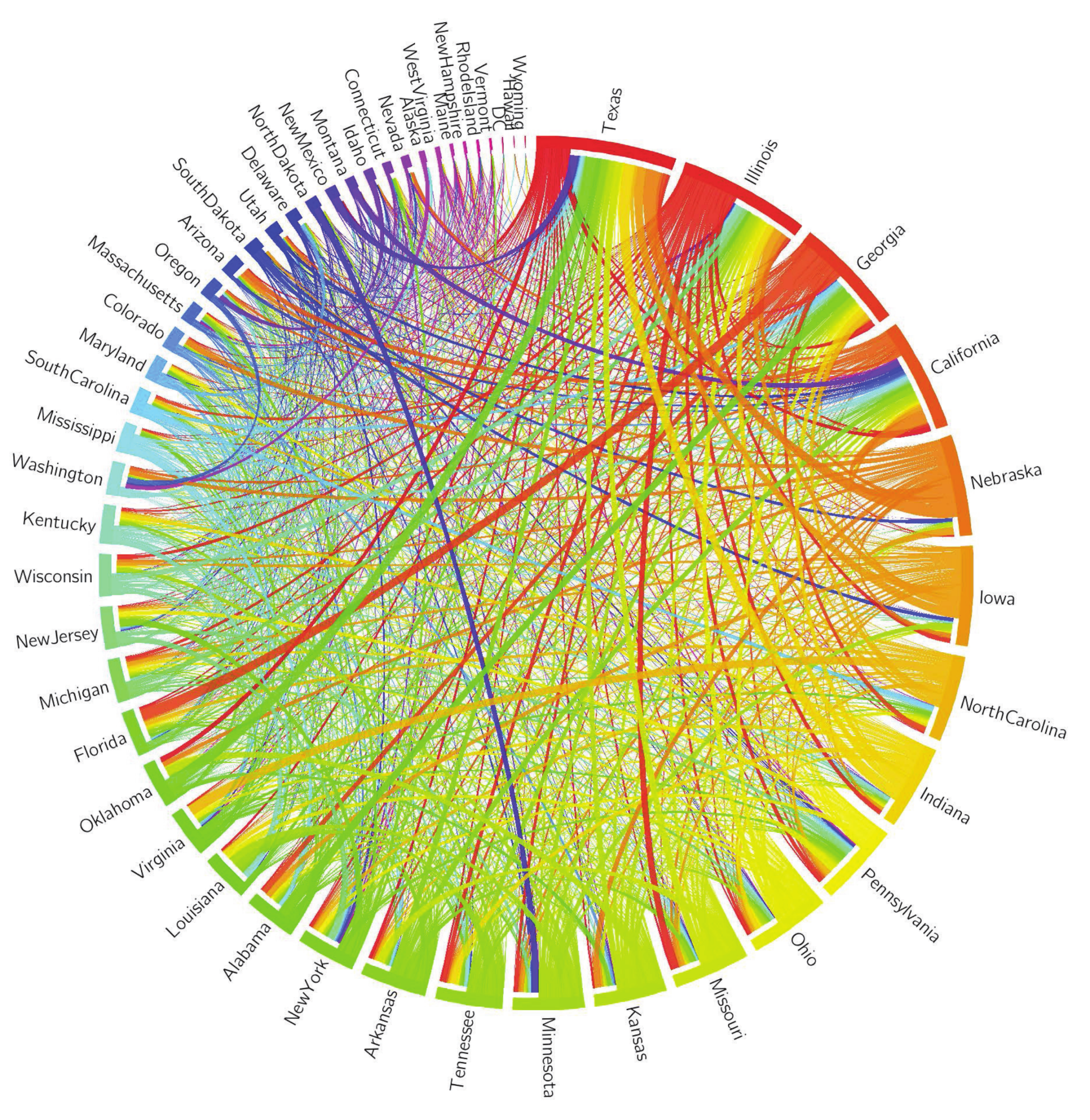
The VWF associated with agriculture has been characterized throughout the United States [27,56]. Figure 2 illustrates the movement of agricultural virtual water flows within the US. The volume of agricultural virtual water flows in 2007 was 317 billion m3, which is over half that of international trade, highlighting the enormous volume of sub-national virtual water flows [56]. The actual volume is much greater since Dang et al. [56] only account for agricultural virtual water flows. Texas has the largest inflows of virtual water, with California, Illinois, and Georgia all major recipients of virtual water. Nebraska sends out the most virtual water, closely followed by other states in the US. Midwest through staple crop commodities [56].
AYH quantified the virtual water trade in energy commodities [58]. Following his lead, studies have examined virtual water flows associated with energy systems in the US. Virtual water transfers associated with domestic ethanol supply chains highlight water risks to energy systems [59]. Virtual water transfers in both food and energy crops have been comprehensively evaluated to provide a complete picture of the US Food–Energy–Water (FEW) system [60], highlighting the tight coupling of these resources. The energy embodied in blue virtual water transfers further fleshes out the national FEW system [61]. The GHG emissions embodied in blue virtual water transfers are comparable to CO2 emissions from the US cement industry, highlighting the importance of reducing the environmental impacts of irrigation [61]. Water is consumed in the generation of electricity and then virtually transmitted across the electric grid [57]. Information on electricity transfers between power control areas and power-plant-level water for electricity are combined to quantify virtual water transfers of electricity. Despite national reductions in freshwater withdrawals for thermoelectric power generation, blue and grey virtual water transfers have increased over time.
Industrial VWF have been evaluated and highlight the important role of cities [62]. There has been much recent work to understand virtual water flows to cities. This requires focusing on the supply chains of cities in the United States and the water footprint of production in the source location. This literature represents the integration of the water footprint community with urban metabolism literature. The CFS/FAF databases provide commodity flow information for several Metropolitan Statistical Areas (MSAs) of the United States, making urban virtual water flow accounting feasible. The virtual water flows to MSAs of the US have been quantified [49], including a comparison between their direct and indirect water use [52]. Full virtual water supply chains associated with both food and energy receipts have been analyzed [63]. Urban virtual water receipts enable the exposure of urban supply chains to water stress to be determined [63,64].
Research on sub-national VWF has considered a different source of water (e.g., green, blue) [56]. Recent work tries to segment the source of water even further, with a particular focus on determining the unsustainable water use. A groundwater model was paired with domestic commodity flow information to estimate the groundwater depletion incorporated in domestic transfers and international exports from the US [21]. The portion of unsustainable surface water irrigation attributable to livestock production through irrigated feed was assessed in recent work [20]. Temporary, rotational fallowing of irrigated feed crops could reduce unsustainable irrigation from surface sources, thereby improving environmental flows [20]. The unsustainable portion of virtual water flows is particularly important to determine because these supply chains face water security risks in the future. For example, agricultural production that depends on unsustainable groundwater use will eventually become infeasible, once groundwater pumping reaches the physical or economic pumping constraints. This makes it important to understand the risks posed to domestic and international agricultural supply chains from the eventual production declines in these locations [21].
It is increasingly important to understand virtual water flows from specific water bodies [22,23,34]. Focusing on water bodies can help to evaluate locations where economic production is aligned with hydrologic budgets. For example, a study of the Great Lakes found that withdrawals do not create significant impacts on surface waters but local, large water uses could create environmental flow impacts [22]. Commercial water uses are the most productive in the Great Lakes, while thermoelectric, mining, and agricultural uses have substantially lower water productivity [22], highlighting potential future pathways to prioritize water allocation. A study of the major aquifers in the US highlights that the water that is unsustainably used for agriculture underpins complex domestic and international supply chains [23]. This highlights a key risk for these agricultural supply chains in the future, as unsustainable groundwater sources will not be able to be used for continued economic production indefinitely.
A major motivation for studying sub-national virtual water flows is to understand how changes and shocks impact producers and consumers. This makes it important to resolve virtual water flows in time to evaluate their evolution and potential disruptions from shocks. For example, paired economic and water footprint models have been used to determine how policy and future climate changes influence global virtual water trade [65,66]. Recent work developed methods to understand the impact of drought on sub-national virtual water transfers [34]. A study of the Central Valley Aquifer in California quantified the impact of the 2012–2015 drought on the water footprint of production and virtual water outflows at the annual time step [34]. Figure 3 shows that green and surface blue virtual water transfers largely decreased from the Central Valley Aquifer to locations around the US and the world. However, groundwater transfers increased following greater reliance on groundwater irrigation from the Central Valley Aquifer during the drought [34].
Virtual Water Storage (VWS) is another important component of the virtual water balance. AYH suggested that storing water in virtual form may be a more efficient and environmentally friendly way of bridging drought periods than building dams [67]. However, until recently, relatively little work has been done to empirically characterize VWS, particularly at the subnational scale. Recently, a statistical assessment of the spatiotemporal patterns of VWS in the United States highlighted the large volume of water stored in grain silos [68]. The VWS in grain was 728 billion m3 in 2012, which is approximately 60% as much water as is stored in US dams. This volume represents 75–97% of precipitation receipts to agricultural areas, depending on the year. Most VWS is from green water (86%) and is in the US Midwest, where there is large grain storage and plentiful rainfall. This work highlights our need to better understand how much water we have stored in stocks of food, energy, and industrial commodities. These VWS stocks may prove important buffers to climate extremes and production shortfalls in the future, making it important to consider their dynamic interaction with virtual water flows.
4. The Water Footprint of Consumption
The water footprint of consumption is the total volume of freshwater consumed and polluted for the production of the goods and services consumed within a certain location (e.g., city, region, or country) [2]. It is calculated by adding the direct water use by people to their indirect water use. The latter can be found by multiplying all goods and services consumed by their respective water footprint.
Several studies have built upon AYH’s definitions and methods to explore the water footprint of consumption of US cities [49,69]. Note that there has long been an interest in the water footprint of US cities that predate AYH’s influence and uses different approaches [70,71]. The average urban water footprint of consumption is roughly 6200 m3/year [52]. The indirect water footprint of a city is 20 times larger than its direct water footprint of consumption [52]. Water embedded within food constitutes over four-fifths of the indirect water footprint of consumption of US cities [52]. Fuel and electricity constitute much of the remainder of a city’s indirect water footprint of consumption. The contribution of energy in a city’s water footprint of consumption varies significantly between cities depending on their energy portfolio and its water intensity [48,52]. Due to the unique properties of the electricity grid, the water footprint of electricity consumption varies widely depending on the methodology employed to attribute water consumed in electricity production to the final consumer [48].
Spatial differences are evident in water footprints of consumption since areas are more likely to source goods and services from nearby locations [63,64]. This explains why a city’s local and non-local exposure to water scarcity is often similar, though the degree of this exposure may differ [63]. For instance, the water footprint of consumption of arid western cities is primarily comprised of water used to irrigate nearby food supplied to the city [52,72]. Nonetheless, the trade of products of different origins and water-intensity creates more homogeneous water footprints of consumption than water footprints of production across cities in the US [54]. Additionally, regional differences in water demands for production are smoothed out by per capita demands for final water. Combining AYH’s water footprint methods with multi-regional input-output (MRIO) models highlights the importance of accounting for product interdependencies in the more refined commodities of cities in order to avoid truncation errors [54].
The typical American adult’s food habits (e.g., diet, food loss and waste) have consequences for energy, water, land, and fertilizer requirements (inputs) and greenhouse gas emissions (outputs) [73,74,75]. If Americans ate a healthier diet, it may be feasible to reduce their blue water consumption by about 4% [74], although shifting to a healthier diet does not always translate into water savings [76]. Dietary shifts to a vegan or vegetarian diet would provide the largest reductions in the consumptive water footprint of the American diet [73,76]. However, reducing food loss and waste would lead to the largest reduction in water use in the US food system [76]. Food loss and waste accounts for approximately 34% of blue water use in the US [74]. So, a combination of measures that include dietary changes and reducing food waste could result in a significant decline in the US water footprint [74,76].
5. Metrics
AYH developed the water footprint concept, “to assess water use along supply chains, sustainability of water use within river basins, efficiency of water use, equitability of water allocation, and dependency on water in the supply chain” [17]. Several studies have built upon these themes in AYH’s research to evaluate how virtual water transfers influence outcomes of interest in the US, including interdependencies, sustainability, security, resilience, and equity.
Researchers have developed approaches to quantify how virtual water flows are linked to other parts of the economy. Rushforth et al. [77] presents a generalized footprint methodology that accounts for the direct and indirect impact of a process on an arbitrarily defined resource. This approach can be used to establish the linkages across footprint types, such as water, ecological, and carbon footprints [77]. Dependencies in the FEW systems have been established, using sub-national virtual water transfers to link the systems together [78]. Domestic commodity flows are driven by geographical proximity [79] which introduces spatially-correlated risks into FEW supply chains. For example, Kansas, Oklahoma, Nebraska, New Mexico and Texas all exhibit strong transfer dependencies and an overreliance on the High Plain aquifer for irrigation. This poses a risk to water shortage in the food supply of Texas, not only through its own production but through its regional agri-food supply chain [78].
The creation of appropriate footprint standards that function as sustainability metrics provide the necessary information for resource managers [77]. Explicitly determining the unsustainable water use throughout a supply chain provides insight into the mass and value of goods that are driving this unsustainable resource extraction [20,21]. In turn, this enables supply chain managers to determine the goods in the supply chain that may be vulnerable to future production losses, when unsustainable water inputs are no longer available. Recent work by AYH and his colleagues has linked US feed production for cattle to surface flow depletion and related environmental flow losses [20] (Figure 4). Water markets may be one solution to curb unsustainable water use in certain river basins [80]. Groundwater depletion in agricultural production highlights risks to future agricultural supply chains [21]. Potential solutions includes voluntary groundwater extraction limits (e.g., Locally Enhanced Management Areas in Kansas [81]), taxes (e.g., San Luis Valley in Colorado [82]), or statewide policy (e.g., the California Sustainable Groundwater Management Act).
Water availability assessment metrics have been presented for green water throughout the US [32]. An integrated assessment of water footprint-derived water security indicators was presented to map the most water-stressed regions throughout the US [10,11]. These indicators reveal the dependencies between human water consumption, crop water requirements, and environmental flows [11]. For example, both the California and Colorado River Basins exhibit severe water scarcity. Yet, water scarcity in the Colorado River Basin is predominantly driven by a decrease in blue water availability, while higher water demands are the main factor in California [11]. Water scarcity and stress are only one dimension of the complex local water context. Threshold-based water footprints have been introduced to enable sustainability indexing that accounts for the local context of water [83]. Importantly, threshold-based footprints account for the unique physical, social, and political dimensions of water resources [83].
Much of the interest in quantifying the virtual water inflows to cities is to determine if urban supply chains are vulnerable. Specifically, methods have been developed to determine the hydro-economic vulnerability and resiliency of a city [64]. Flagstaff’s virtual water receipts were shown to increase both its hydro-economic resilience and vulnerability to water scarcity in the locations of production [64]. Building on these methods, studies have evaluated the water scarcity exposure of urban FEW receipts for all cities in the US, based on their virtual water inflows [63]. Cities typically import commodities from nearby locations with similar water resource constraints. This means that urban FEW supply chains are generally exposed to spatially correlated water scarcity risks [63]. For example, cities in the western US have scarce local water resources and also import commodities from other water-scarce western locations [63]. This understanding can help city operators coordinate with supply chain managers to minimize risk.
The equality of virtual water flows has been assessed within the US and compared to the global virtual water trade [56]. Flows within the United States are more equitable than they are globally. However, the United States still do not exhibit perfectly equitable virtual water flows. The United States does not have barriers to trade, has a shared national agricultural policy, a national currency, and is relatively wealthy. If virtual water flows do not achieve perfect equality within the US then it is unlikely—and potentially even undesirable—that global virtual trade will be able to achieve perfect equality. We suggest that future research examines equality in food access and consumption, rather than evaluating equality of virtual water flows. Going forward, it is important to explicitly acknowledge the socio-political judgments regarding the values assigned when modeling virtual water resources [83].
6. Future Research Directions
“The interest in the water footprint is rooted in the recognition that human impacts on freshwater systems can ultimately be linked to human consumption, and that issues like water shortages and pollution can be better understood and addressed by considering production and supply chains as a whole.”—Arjen Y. Hoekstra
Arjen Y. Hoekstra recognized that water issues and solutions are highly-localized, yet driven by a complex global system of production and consumption. His research reflected this understanding through his study of systems whose boundaries extended beyond the watershed, yet provided sufficient detail to understand hydrologic fluxes and impacts at these smaller scales. In our increasingly globalized world, AYH provided a timely new approach to understanding local-to-global connections between water and society. While issues of water scarcity, degradation, and depletion have long been studied, AYH prompted a new era of researchers to investigate the global drivers of these issues. A community of scholars has sought to understand these questions within the US. How does global trade and consumption drive unsustainable water use? [21,22,23,34]. How do our dietary choices impact streamflow and riverine ecosystems? [9,10,11,20,22,53]. Where are our supply chains at risk due to water stress and drought? [20,34,63,64,84,85].
Governments, corporations, and individuals have taken measures to reduce their water footprint based on AYH’s work. AYH’s vision for the water footprint concept was not strictly an exercise in academic curiosity, but one rooted in bringing new solutions to the water issues facing society, such as water basin caps [86]. To this end, several researchers, including AYH, have proposed and evaluated means to reduce water consumption and the environmental and societal harms associated with the exploitation of this natural resource in the US and beyond. For instance, streamflow depletion in the Western US can be reduced by as much as 23% by shifting unproductive water users to their industry-specific benchmark of water-productivity [53] (Figure 5). A fallowing schedule for irrigated cropland in water-stressed basins and more water-conscious cropping patterns can preserve water for the environment and high-value water uses [20,36]. Most companies could reduce their water footprint more by working with their upstream suppliers than by solely adjusting their internal processes [4,53]. It is important for decision-makers to consider the full life-cycle water use of technological solutions to water stress, to avoid unintended consequences that may actually intensify water stress [87,88]. We can all reduce our water footprint by adopting a less water-intensive diet [20,59,76] and wasting less food [74,76,89].
Sound decision-making and solutions to US water issues are founded on solid science, which is underpinned by data of sufficient quality and at the appropriate level of detail. The majority of water uses in the US are not metered, meaning that water footprint data is largely based on models and proxies for water use. Multiple approaches to estimate water use are needed to triangulate the water demands of society and the environment. Remote sensing data products can be used to estimate water use at fine spatial resolutions over large areas. Remote sensing products can be validated against flux towers and locations with metered water use. These data can be used to improve process-based and empirical models of water use. Together, these data and models can be harnessed by process-guided machine learning algorithms to improve water footprint estimates and provide new insights into the drivers of water use. Importantly, future water footprint and virtual water research must better quantify the uncertainty inherent in the underlying data and models [4,90].
How have water footprints in the United States changed over time? We require more refined temporal estimates of water footprints over long periods of time to answer this question. Additionally, to enable footprint estimates to be used for real-time or near real-time decision-making, we require a significant reduction in the latency of input data. To date, most studies have used temporally averaged water footprint estimates, which conceal the significant intra- and inter-annual variability of water footprints. There is often a multi-year lag between water footprint assessments and the actual occurrence of water use due to time delays between data collection and dissemination of these data. The USGS and other groups are working to streamline their water use data collection and dissemination [91]. These data, along with near real-time remote sensing products, can significantly shorten the time lag between water use and water footprint research to enable decision making.
The first water footprint studies were typically at the national or regional scale, thereby offering a coarse understanding of where water was used. Most US studies now use sub-national data (see Table 1), often at the county or city level or even finer spatial resolutions. This giant step forward in the spatial detail of water footprint studies was accelerated by the publication of several high-resolution water footprint datasets by AYH [4,92,93,94,95,96]. The next leap forward in water footprint assessments will require more than a continued refinement of existing models and methods. New data products and methods to capture heterogeneity between water users at the field or facility level will lead to a new understanding of the behavioral, regulatory, economic, infrastructure, and policy drivers of water use. The next generation of water footprint assessments will provide more precise estimates of water consumption and also connect water footprints to specific water sources through infrastructure (e.g., diversion intakes, groundwater wells, irrigation canals, interbasin water transfers [97]). Different irrigation technologies and management strategies (e.g., deficit irrigation) need to be accounted for within water footprint estimates. This will allow for a more accurate representation of the water consumed in the production of irrigated agriculture by accounting for water consumed throughout the entire production system (i.e., evaporation from canals, inefficient irrigation operations, as well as plant transpiration). Future research should focus on improving our understanding of agricultural water use, given this sector’s outsized water footprint. However, the industrial and commercial sectors are particularly ripe for additional research, as these sectors have not been the focus of as much research in the literature.
Advances in the temporal and spatial dimensions of water footprint assessments can improve large scale hydrologic models and integrated assessment models. Detailed water footprint estimates or a new understanding of the drivers of water use can be incorporated within hydrologic models to see how water consumption impacts streamflow and aquifer conditions. This could then be paired with economic or ecological models to understand how changes in water demands, either directly through water-intensive production or indirectly through supply chains (i.e., virtual water transfers), alter ecological flows, or other water users. If paired with information on water rights and priorities, one could even determine those most at risk during drought of not being able to fulfill their water rights or have disruptions in their supply chains. Pairing water footprints with other environmental footprint metrics, as well as economic and social impact assessments, will provide a more holistic analysis of society’s production and consumption patterns and the implications of mitigation strategies [98].
Trade influences domestic water use and virtual water trade [8,15,66], making it important to guide policy in future research. To better assess the interaction between supply chains and water resources we need fine-grained commodity flow information. For this reason, recent research has developed methods to map food flows between counties in the US [79]. Future work can build on this to model food supply chains in time and determine the critical infrastructure that enables virtual water flows. Additionally, future work could link water footprint and input-output methods to more accurately determine how water is incorporated into the full production chain. The integration of water footprint and input-output methods could be done in a manner that spatializes water use as it is transformed into refined commodities and economic sectors, drawing on the strengths of both research communities. All of these approaches would help us to better account for water use throughout the full supply chain. However, to understand the causal relationships that exist between water use and supply chains, econometric methods that properly account for selection bias in complex human systems need to be used. For example, the econometric methods that were used to determine the impact of trade on water and nutrient use at a global scale [8,99] could be implemented within the United States.
7. Concluding Remarks
Arjen reshaped the way the world thinks about water. His impact on our research and the research of countless others is a testament to his genius and his generous sharing of ideas and data. Together, let us strive to carry on Arjen’s passionate pursuit of a more sustainable, equitable, and efficient [103] use of the world’s freshwater.
Author Contributions
M.K. and L.M. contributed equally to the writing of this paper. All authors have read and agreed to the published version of the manuscript.
Funding
This material is based upon work supported by the National Science Foundation Grants ACI-1639529 (“INFEWS/T1: Mesoscale Data Fusion to Map and Model the U.S. Food, Energy, and Water (FEW) System”), EAR-1534544 (“Hazards SEES: Understanding Cross-Scale Interactions of Trade and Food Policy to Improve Resilience to Drought Risk”), and CBET-1844773 (“CAREER: A National Strategy for a Resilient Food Supply Chain”), as well as U.S. Geological Survey Grant/Cooperative Agreement No. G20AP00002 (“Mapping and modeling of interbasin water transfers within the United States”) and the U.S. Geological Survey John Wesley Powell Center for Analysis and Synthesis supported working group project (“Reanalyzing and Predicting U.S. Water Use using Economic History and Forecast Data; an experiment in short-range national hydro-economic data synthesis”). Any opinions, findings, and conclusions or recommendations expressed in this material are those of the author(s) and do not necessarily reflect the views of the National Science Foundation or the U.S. Geological Survey.
Acknowledgments
We wrote this paper to commemorate Arjen Y. Hoekstra on the one-year anniversary of his untimely death. He was a huge inspiration and enabler of our work. We thank Paul J. Ruess, Deniz Berfin Karakoc, Junren Wang, Md. Abu Bakar Siddik, and Akshay Pandit for help with the literature review.
Conflicts of Interest
The authors declare no conflict of interest.
Abbreviations
The following abbreviations are used in this manuscript:
| AYH | Arjen Y. Hoekstra |
| WF | Water Footprint |
| VWT | Virtual Water Trade |
| VWF | Virtual Water Flow |
| VWS | Virtual Water Storage |
| CFS | Commodity Flow Survey |
| FAF | Freight Analysis Framework |
| MRIO | Multi-Region Input-Output |
| MSA | Metropolitan Statistical Area |
| FEW | Food-Energy-Water |
| USGS | US Geological Survey |
References
- Hoekstra, A.Y.; Hung, P. Virtual Water Trade: A Quantification of Virtual Water Flows between Nations in Relation to International Crop Trade; UNESCO-IHE Institute for Water Education: Delft, The Netherlands, 2002. [Google Scholar]
- Hoekstra, A.Y.; Chapagain, A.K. Globalization of Water: Sharing the Planet’s Freshwater Resources; Wiley-Blackwell: Hoboken, NJ, USA, 2008; p. 220. [Google Scholar]
- Hoekstra, A.Y.; Mekonnen, M.M. The water footprint of humanity. Proc. Natl. Acad. Sci. USA 2012, 109, 3232–3237. [Google Scholar] [CrossRef] [PubMed] [Green Version]
- Marston, L.; Ao, Y.; Konar, M.; Mekonnen, M.M.; Hoekstra, A.Y. High-resolution water footprints of production of the United States. Water Resour. Res. 2018, 54, 2288–2316. [Google Scholar] [CrossRef]
- Konar, M.; Dalin, C.; Suweis, S.; Hanasaki, N.; Rinaldo, A.; Rodriguez-Iturbe, I. Water for food: The global virtual water trade network. Water Resour. Res. 2011, 47, W05520. [Google Scholar] [CrossRef] [Green Version]
- Xu, M.; Allenby, B.R.; Crittenden, J.C. Interconnectedness and resilience of the U.S. economy. Adv. Complex Syst. 2011, 14, 649–672. [Google Scholar] [CrossRef]
- Devineni, N.; Lall, U.; Etienne, E.; Shi, D.; Xi, C. America’s water risk: Current demand and climate variability. Geophys. Res. Lett. 2015, 42, 2285–2293. [Google Scholar] [CrossRef]
- Dang, Q.; Konar, M. Trade Openness and Domestic Water Use. Water Resour. Res. 2018, 54, 4–18. [Google Scholar] [CrossRef] [Green Version]
- Veettil, A.V.; Mishra, A. Water security assessment using blue and green water footprint concepts. J. Hydrol. 2016, 542, 589–602. [Google Scholar] [CrossRef]
- Veettil, A.V.; Mishra, A. Potential influence of climate and anthropogenic variables on water security using blue and green water scarcity, Falkenmark index, and freshwater provision indicator. J. Environ. Manag. 2018, 228, 346–362. [Google Scholar] [CrossRef]
- Veettil, A.V.; Mishra, A. Water security assessment for the contiguous United States using water footprint concepts. Geophys. Res. Lett. 2020, 45, e2020GL087061. [Google Scholar] [CrossRef]
- Dieter, C.; Maupin, M.; Caldwell, R.; Harris, M.; Ivahnenko, T.; Lovelace, J.; Barber, N.; Linsey, K. Estimated use of water in the United States in 2015. In U.S. Geological Survey Circular 1441; U.S. Geological Survey: Reston, VA, USA, 2018; p. 65. [Google Scholar] [CrossRef]
- Perrone, D.; Hornberger, G.; van Vliet, O.; van der Velde, M. A review of the United States’ past and projected water use. J. Am. Water Resour. Assoc. 2015, 51, 1183–1191. [Google Scholar] [CrossRef]
- Debaere, P.; Kurzendoerfer, A. Decomposing US Water Withdrawal since 1950. JAERE 2017, 4, 155–196. [Google Scholar] [CrossRef]
- Avelino, A.F.T.; Dall’erba, S. What Factors Drive the Changes in Water Withdrawals in the U.S. Agriculture and Food Manufacturing Industries between 1995 and 2010? Environ. Sci. Technol. 2020, 54, 10421–10434. [Google Scholar] [CrossRef] [PubMed]
- Worland, S.C.; Steinschneider, S.; Hornberger, G.M. Drivers of Variability in Public-Supply Water Use Across the Contiguous United States. Water Resour. Res. 2018, 54, 1868–1889. [Google Scholar] [CrossRef]
- Hoekstra, A.Y. A critique on the water-scarcity weighted water footprint in LCA. Ecol. Indic. 2016, 66, 564–573. [Google Scholar] [CrossRef] [Green Version]
- Hoekstra, A.Y.; Chapagain, A.K.; Mekonnen, M.M.; Aldaya, M.M. The Water Footprint Assessment Manual: Setting the Global Standard; Routledge: Abingdon, UK, 2011. [Google Scholar]
- Grubert, E.; Sanders, K.T. Water Use in the United States Energy System: A National Assessment and Unit Process Inventory of Water Consumption and Withdrawals. Environ. Sci. Technol. 2018, 52, 6695–6703. [Google Scholar] [CrossRef]
- Richter, B.D.; Bartak, D.; Caldwell, P.; Davis, K.F.; Debaere, P.; Hoekstra, A.Y.; Li, T.; Marston, L.; McManamay, R.; Mekonnen, M.M.; et al. Water scarcity and fish imperilment driven by beef production. Nat. Sustain. 2020, 3, 319–328. [Google Scholar] [CrossRef]
- Gumidyala, S.; Ruess, P.J.; Konar, M.; Marston, L.; Dalin, C.; Wada, Y. Groundwater depletion embedded in domestic transfers and international exports of the United States. Water Resour. Res. 2020, 56. [Google Scholar] [CrossRef] [Green Version]
- Mayer, A.; Mubako, S.; Ruddell, B.L. Developing the greatest Blue Economy: Water productivity, fresh water depletion, and virtual water trade in the Great Lakes basin. Earth’s Future 2016, 4, 282–297. [Google Scholar] [CrossRef] [Green Version]
- Marston, L.; Konar, M.; Cai, X.; Troy, T.J. Virtual groundwater transfers from overexploited aquifers in the United States. Proc. Natl. Acad. Sci. USA 2015, 112, 8561–8566. [Google Scholar] [CrossRef] [Green Version]
- Rushforth, R.R.; Ruddell, B.L. A spatially detailed blue water footprint of the United States economy. Hydrol. Earth Syst. Sci. 2018, 22, 3007. [Google Scholar] [CrossRef] [Green Version]
- Zhuo, L.; Hoekstra, A.Y. The effect of different agricultural management practices on irrigation efficiency, water use efficiency and green and blue water footprint. Front. Agric. Sci. Eng. 2017, 4, 185–194. [Google Scholar] [CrossRef] [Green Version]
- Nouri, H.; Stokvis, B.; Galindo, A.; Blatchford, M.; Hoekstra, A.Y. Water scarcity alleviation through water footprint reduction in agriculture: the effect of soil mulching and drip irrigation. Sci. Total Environ. 2019, 653, 241–252. [Google Scholar] [CrossRef] [PubMed]
- Mubako, S.T.; Lant, C.L. Agricultural virtual water trade and water footprint of US states. Ann. Assoc. Am. Geogr. 2013, 103, 385–396. [Google Scholar] [CrossRef]
- Fulton, J.; Norton, M.; Shillingb, F. Water-indexed benefits and impacts of California almonds. Ecol. Indic. 2019, 96, 711–717. [Google Scholar] [CrossRef]
- Mekonnen, M.M.; Neale, C.M.; Ray, C.; Erickson, G.E.; Hoekstra, A.Y. Water productivity in meat and milk production in the US from 1960 to 2016. Environ. Int. 2019, 132, 105084. [Google Scholar] [CrossRef] [PubMed]
- Schyns, J.F.; Hoekstra, A.Y.; Booij, M.J. Review and classification of indicators of green water availability and scarcity. Hydrol. Earth Syst. Sci. 2015, 19, 4581–4608. [Google Scholar] [CrossRef] [Green Version]
- Schyns, J.F.; Hoekstra, A.Y.; Booij, M.J.; Hogeboom, R.J.; Mekonnen, M.M. Limits to the world’s green water resources for food, feed, fiber, timber, and bioenergy. Proc. Natl. Acad. Sci. USA 2019, 116, 4893–4898. [Google Scholar] [CrossRef] [Green Version]
- Xu, H.; Wu, M. A First Estimation of County-Based Green Water Availability and Its Implications for Agriculture and Bioenergy Production in the United States. Water 2018, 10, 148. [Google Scholar] [CrossRef] [Green Version]
- Xu, H.; Wu, M.; Ha, M. A county-level estimation of renewable surface water and groundwater availability associated with potential large-scale bioenergy feedstock production scenarios in the United States. GCB Bioenergy 2019, 11, 606–622. [Google Scholar] [CrossRef] [Green Version]
- Marston, L.; Konar, M. Drought impacts to water footprints and virtual water transfers of the Central Valley of California. Water Resour. Res. 2017, 53, 5756–5773. [Google Scholar] [CrossRef]
- Fulton, J.; Cooley, H.; Gleick, P.H. Water Footprint Outcomes and Policy Relevance Change with Scale Considered: Evidence from California. Water Resour. Manag. 2014, 28, 3637–3649. [Google Scholar] [CrossRef]
- Davis, K.F.; Seveso, A.; Rulli, M.C.; D’Odorico, P. Water Savings of Crop Redistribution in the United States. Water 2017, 9, 83. [Google Scholar] [CrossRef] [Green Version]
- Dominguez-Faus, R.; Powers, S.E.; Burken, J.G.; Alvarez, P.J. The water footprint of biofuels: A drink or drive issue? Environ. Sci. Technol. 2009, 43, 3005–3010. [Google Scholar] [CrossRef] [PubMed] [Green Version]
- Cai, X.; Wallington, K.; Shafiee-Jood, M.; Marston, L. Understanding and managing the food-energy-water nexus–opportunities for water resources research. Adv. Water Resour. 2018, 111, 259–273. [Google Scholar] [CrossRef]
- Chiu, Y.W.; Wu, M. Assessing county-level water footprints of different cellulosic-biofuel feedstock pathways. Environ. Sci. Technol. 2012, 46, 9155–9162. [Google Scholar] [CrossRef] [Green Version]
- Scown, C.D.; Horvath, A.; McKone, T.E. Water Footprint of U.S. Transportation Fuels. Environ. Sci. Technol. 2011, 45, 2541–2553. [Google Scholar] [CrossRef]
- Kondash, A.J.; Lauer, N.E.; Vengoshn, A. The intensification of the water footprint of hydraulic fracturing. Sci. Adv. 2018, 4, eaar5982. [Google Scholar] [CrossRef] [Green Version]
- Kondash, A.J.; Vengoshn, A. Water Footprint of Hydraulic Fracturing. Environ. Sci. Technol. Lett. 2015, 2, 276–280. [Google Scholar] [CrossRef]
- Scanlon, B.R.; Reedy, R.C.; Male, F.; Hove, M. Managing the Increasing Water Footprint of Hydraulic Fracturing in the Bakken Play, United States. Environ. Sci. Technol. 2016, 50, 10273–10281. [Google Scholar] [CrossRef]
- Chini, C.M.; Logan, L.H.; Stillwell, A.S. Grey Water Footprints of US Thermoelectric Power Plants from 2010–2016. Adv. Water Resour. 2020, 145, 103733. [Google Scholar] [CrossRef]
- Hogeboom, R.J.; Knook, L.; Hoekstra, A.Y. The blue water footprint of the world’s artificial reservoirs for hydroelectricity, irrigation, residential and industrial water supply, flood protection, fishing and recreation. Adv. Water Resour. 2018, 113, 285–294. [Google Scholar] [CrossRef]
- Mekonnen, M.; Hoekstra, A.Y.; Thompson, S. The blue water footprint of electricity from hydropower. Hydrol. Earth Syst. Sci. 2012, 16, 179–187. [Google Scholar] [CrossRef] [Green Version]
- Grubert, E.A. Water consumption from hydroelectricity in the United States. Adv. Water Resour. 2016, 96, 88–94. [Google Scholar] [CrossRef] [Green Version]
- Siddik, M.A.B.; Chini, C.M.; Marston, L. Water and Carbon Footprints of Electricity Are Sensitive to Geographical Attribution Methods. Environ. Sci. Technol. 2020, 54, 7533–7541. [Google Scholar] [CrossRef] [PubMed]
- Ahams, I.C.; Paterson, W.; Garcia, S.; Rushforth, R.; Ruddell, B.L.; Mejia, A. Water footprint of 65 mid- to large-sized U.S. cities and their metropolitan areas. J. Am. Water Resour. Assoc. 2017, 53, 1147–1163. [Google Scholar] [CrossRef]
- Moore, B.C.; Coleman, A.M.; Wigmosta, M.S.; Skaggs, R.L.; Venteris, E.R. A High Spatiotemporal Assessment of Consumptive Water Use and Water Scarcity in the Conterminous United States. Water Resour. Manag. 2015, 29, 5185–5200. [Google Scholar] [CrossRef]
- Mubako, S.; Lahiri, S.; Lant, C. Input–output analysis of virtual water transfers: Case study of California and Illinois. Ecol. Econ. 2013, 93, 230–238. [Google Scholar] [CrossRef]
- Chini, C.M.; Konar, M.; Stillwell, A.S. Direct and indirect urban water footprints of the United States. Water Resour. Res. 2017, 53, 316–327. [Google Scholar] [CrossRef]
- Marston, L.T.; Lamsal, G.; Ancona, Z.H.; Caldwell, P.; Richter, B.D.; Ruddell, B.L.; Rushforth, R.R.; Davis, K.F. Reducing water scarcity by improving water productivity in the United States. Environ. Res. Lett. 2020, 15, 094033. [Google Scholar] [CrossRef]
- Garcia, S.; Rushforth, R.; Ruddell, B.L.; Mejia, A. Full domestic supply chains of blue virtual water flows estimated for major US cities. Water Resour. Res. 2020, 56, e2019WR026190. [Google Scholar] [CrossRef]
- Bae, J.; Dall’Erba, S. Crop production, export of virtual water and water-saving strategies in Arizona. Ecol. Econ. 2018, 146, 148–156. [Google Scholar] [CrossRef]
- Dang, Q.; Lin, X.; Konar, M. Agricultural virtual water flows within the United States. Water Resour. Res. 2015, 51, 973–986. [Google Scholar] [CrossRef]
- Chini, C.M.; Djehdian, L.A.; Lubega, W.N.; Stillwell, A.S. Virtual water transfers of the US electric grid. Nat. Energy 2018, 3, 1115–1123. [Google Scholar] [CrossRef]
- Gerbens-Leenes, W.; Hoekstra, A.Y.; van der Meer, T.H. The water footprint of bioenergy. Proc. Natl. Acad. Sci. USA 2009, 106. [Google Scholar] [CrossRef] [PubMed] [Green Version]
- Brauman, K.A.; Goodkind, A.L.; Kim, T.; Pelton, R.; Schmitt, J.; Smith, T. Unique water scarcity footprints and water risks in US meat and ethanol supply chains identified via subnational commodity flows. Environ. Res. Lett. 2020. [Google Scholar] [CrossRef]
- Mahjabin, T.; Mejia, A.; Blumsack, S.; Grady, C. Integrating embedded resources and network analysis to understand food-energy-water nexus in the US. Sci. Total Environ. 2020, 709, 136153. [Google Scholar] [CrossRef]
- Vora, N.; Shah, A.; Bilec, M.M.; Khanna, V. Food–energy–water nexus: Quantifying embodied energy and GHG emissions from irrigation through virtual water transfers in food trade. ACS Sustain. Chem. Eng. 2017, 5, 2119–2128. [Google Scholar] [CrossRef]
- Garcia, S.; Mejia, A. Characterizing and modeling subnational virtual water networks of US agricultural and industrial commodity flows. Adv. Water Resour. 2019, 130, 314–324. [Google Scholar] [CrossRef]
- Djehdian, L.A.; Chini, C.M.; Marston, L.; Konar, M.; Stillwell, A.S. Exposure of urban food–energy–water (FEW) systems to water scarcity. Sustain. Cities Soc. 2019, 50, 101621. [Google Scholar] [CrossRef]
- Rushforth, R.R.; Ruddell, B.L. The vulnerability and resilience of a city’s water footprint: The case of Flagstaff, Arizona, USA. Water Resour. Res. 2016, 52, 2698–2714. [Google Scholar] [CrossRef] [Green Version]
- Konar, M.; Hussein, Z.; Hanasaki, N.; Mauzerall, D.L.; Rodriguez-Iturbe, I. Virtual water trade flows and savings under climate change. Hydrol. Earth Syst. Sci. 2013, 17, 3219–3234. [Google Scholar] [CrossRef] [Green Version]
- Konar, M.; Reimer, J.; Hussein, Z.; Hanasaki, N. The water footprint of staple crop trade under climate and policy scenarios. Environ. Res. Lett. 2016, 11, 035006. [Google Scholar] [CrossRef] [Green Version]
- Hoekstra, A.Y. Virtual Water: An Introduction, Virtual Water Trade: Proceedings of the International Expert Meeting on Virtual Water Trade; Value of Water Research Report Series; UNESCO-IHE Institute for Water Education: Delft, The Netherlands, 2003. [Google Scholar]
- Ruess, P.J.; Konar, M. Grain and virtual water storage capacity in the United States. Water Resour. Res. 2019, 55, 3960–3975. [Google Scholar] [CrossRef]
- Mahjabin, T.; Garcia, S.; Grady, C.; Mejia, A. Large cities get more for less: Water footprint efficiency across the US. PLoS ONE 2018, 13, e0202301. [Google Scholar] [CrossRef] [PubMed]
- Luck, M.A.; Jenerette, G.D.; Wu, J.; Grimm, N.B. The Urban Funnel Model and the Spatially Heterogeneous Ecological Footprint. Ecosystems 2001, 4, 782–796. [Google Scholar] [CrossRef]
- Jenerette, G.D.; Wu, W.; Goldsmith, S.; Marussich, W.A.; Roach, W.J. Contrasting water footprints of cities in China and the United States. Ecol. Econ. 2006, 57, 346–358. [Google Scholar] [CrossRef]
- Sabo, J.L.; Sinha, T.; Bowling, L.C.; Schoups, G.H.; Wallender, W.W.; Campana, M.E.; Cherkauer, K.A.; Fuller, P.L.; Graf, W.L.; Hopmans, J.W.; et al. Reclaiming freshwater sustainability in the Cadillac Desert. Proc. Natl. Acad. Sci. USA 2010, 107, 21263–21269. [Google Scholar] [CrossRef] [Green Version]
- Blas, A.; Garrido, A.; Willaarts, B.A. Evaluating the Water Footprint of the Mediterranean and American Diets. Water 2016, 8, 448. [Google Scholar] [CrossRef] [Green Version]
- Birney, C.I.; Franklin, K.F.; Davidson, F.T.; Webber, M.E. An assessment of individual foodprints attributed to diets and food waste in the United States. Environ. Res. Lett. 2017, 12, 105008. [Google Scholar] [CrossRef]
- Kim, B.F.; Santo, R.E.; Scatterday, A.P.; Fry, J.P.; Synk, C.M.; Cebron, S.R.; Mekonnen, M.M.; Hoekstra, A.Y.; de Pee, S.; Bloem, M.W.; et al. Country-specific dietary shifts to mitigate climate and water crises. Glob. Environ. Chang. 2020, 62. [Google Scholar] [CrossRef]
- Mekonnen, M.M.; Fulton, J. The effect of diet changes and food loss reduction in reducing the water footprint of an average American. Water Int. 2018, 43. [Google Scholar] [CrossRef]
- Rushforth, R.R.; Adams, E.A.; Ruddell, B.L. Generalizing ecological, water and carbon footprint methods and their worldview assumptions using Embedded Resource Accounting. Water Resour. Ind. 2013, 1, 77–90. [Google Scholar] [CrossRef] [Green Version]
- Vora, N.; Fath, B.D.; Khanna, V. A Systems Approach To Assess Trade Dependencies in US Food–Energy–Water Nexus. Environ. Sci. Technol. 2019, 53, 10941–10950. [Google Scholar] [CrossRef] [PubMed]
- Lin, X.; Ruess, P.J.; Marston, L.; Konar, M. Food flows between counties in the United States. Environ. Res. Lett. 2019, 14. [Google Scholar] [CrossRef]
- Debaere, P.; Li, T. The effects of water markets: Evidence from the Rio Grande. Adv. Water Resour. 2020, 145. [Google Scholar] [CrossRef]
- Deines, J.M.; Kendall, A.D.; Butler, J.J.; Hyndman, D.W. Quantifying irrigation adaptation strategies in response to stakeholder-driven groundwater management in the US High Plains Aquifer. Environ. Res. Lett. 2019, 14, 044014. [Google Scholar] [CrossRef]
- Cody, K.C.; Smith, S.M.; Cox, M.; Andersson, K. Emergence of collective action in a groundwater commons: irrigators in the San Luis Valley of Colorado. Soc. Nat. Resour. 2015, 28, 405–422. [Google Scholar] [CrossRef] [Green Version]
- Ruddell, B.L. Threshold Based Footprints (for Water). Water 2018, 10, 1029. [Google Scholar] [CrossRef] [Green Version]
- Ruddell, B.L.; Adams, E.A.; Rushforth, R.; Tidwell, V.C. Embedded resource accounting for coupled natural-human systems: An application to water resource impacts of the western US electrical energy trade. Water Resour. Res. 2014, 50, 7957–7972. [Google Scholar] [CrossRef]
- Rushforth, R.R.; Ruddell, B.L. The hydro-economic interdependency of cities: Virtual water connections of the Phoenix, Arizona Metropolitan Area. Sustainability 2015, 7, 8522–8547. [Google Scholar] [CrossRef] [Green Version]
- Hogeboom, R.J.; de Bruin, D.; Schyns, J.F.; Krol, M.S.; Hoekstra, A.Y. Capping Human Water Footprints in the World’s River Basins. Earth’s Future 2020, 8. [Google Scholar] [CrossRef] [PubMed]
- Haghighi, E.; Madan, K.; Hoekstra, A.Y. The water footprint of water conservation using shade balls in California. Nat. Sustain. 2018, 1, 358–360. [Google Scholar] [CrossRef]
- Pfeiffer, L.; Lin, C.Y.C. Does efficient irrigation technology lead to reduced groundwater extraction? Empirical evidence. J. Environ. Econ. Manag. 2014, 67, 189–208. [Google Scholar] [CrossRef] [Green Version]
- Read, Q.D.; Brown, S.; Cuéllar, A.D.; Finn, S.M.; Gephart, J.A.; Marston, L.T.; Meyer, E.; Weitz, K.A.; Muth, M.K. Assessing the environmental impacts of halving food loss and waste along the food supply chain. Sci. Total Environ. 2020, 712, 136255. [Google Scholar] [CrossRef]
- Zhuo, L.; Mekonnen, M.; Hoekstra, A.Y. Sensitivity and uncertainty in crop water footprint accounting: A case study for the Yellow River basin. Hydrol. Earth Syst. Sci. 2014, 18, 2219. [Google Scholar] [CrossRef] [Green Version]
- Evenson, E.J.; Jones, S.A.; Barber, N.L.; Barlow, P.M.; Blodgett, D.L.; Bruce, B.W.; Douglas-Mankin, K.; Farmer, W.H.; Fischer, J.M.; Hughes, W.B.; et al. Continuing Progress Toward a National Assessment of Water Availability and Use; Technical Report; U.S. Geological Survey: Reston, VA, USA, 2018.
- Mekonnen, M.M.; Hoekstra, A.Y. A global assessment of the water footprint of farm animal products. Ecosystems 2012, 15, 401–415. [Google Scholar] [CrossRef] [Green Version]
- Mekonnen, M.M.; Hoekstra, A.Y. The green, blue and grey water footprint of crops and derived crop products. Hydrol. Earth Syst. Sci. 2011, 15, 1577–1600. [Google Scholar] [CrossRef] [Green Version]
- Mekonnen, M.M.; Hoekstra, A.Y. National Water Footprint Accounts: The Green, Blue and Grey Water Footprint of Production and Consumption. Volume 1: Main Report; UNESCO-IHE: Delft, The Netherlands, 2011. [Google Scholar]
- Mekonnen, M.M.; Hoekstra, A.Y. Four billion people facing severe water scarcity. Sci. Adv. 2016, 2, e1500323. [Google Scholar] [CrossRef] [Green Version]
- Hoekstra, A.Y.; Mekonnen, M.M.; Chapagain, A.K.; Mathews, R.E.; Richter, B.D. Global monthly water scarcity: blue water footprints versus blue water availability. PLoS ONE 2012, 7, e32688. [Google Scholar] [CrossRef]
- Dickson, K.E.; Marston, L.T.; Dzombak, D.A. Editorial Perspectives: the need for a comprehensive, centralized database of interbasin water transfers in the United States. Environ. Sci. Water Res. Technol. 2020, 6, 420–422. [Google Scholar] [CrossRef]
- Vanham, D.; Leip, A.; Galli, A.; Kastner, T.; Bruckner, M.; Uwizeye, A.; Van Dijk, K.; Ercin, E.; Dalin, C.; Bastianoni, S.; et al. Environmental footprint family to address local to planetary sustainability and deliver on the SDGs. Sci. Total Environ. 2019, 693. [Google Scholar] [CrossRef]
- Dang, Q.; Konar, M.; Debaere, P. Trade Openness and The Nutrient Use of Nationas. Environ. Res. Lett. 2018, 13. [Google Scholar] [CrossRef] [Green Version]
- Hoekstra, A.Y. The water footprint of animal products. In The Meat Crisis: Developing More Sustainable Production and Consumption; Taylor & Francis: Abingdon, UK, 2010; pp. 22–33. [Google Scholar]
- Mekonnen, M.M.; Gerbens-Leenes, P.W.; Hoekstra, A.Y. The consumptive water footprint of electricity and heat: a global assessment. Environ. Sci. Water Res. Technol. 2015, 1, 285–297. [Google Scholar] [CrossRef]
- White, M.; Gambone, M.; Yen, H.; Arnold, J.; Harmel, D.; Santhi, C.; Haney, R. Regional blue and green water balances and use by selected crops in the U.S. J. Am. Water Resour. Assoc. 2015, 51. [Google Scholar] [CrossRef]
- Hoekstra, A.Y. Sustainable, efficient, and equitable water use: the three pillars under wise freshwater allocation. Wiley Interdiscip. Rev. Water 2014, 1, 31–40. [Google Scholar] [CrossRef]
Figure 1.
Map of the sector with the largest blue water footprint in each US county. Agriculture is the largest water user in 2164 of the 3143 counties. In other counties, service industries (354), thermoelectric power generation (289), manufacturing (234), and mining (102) are the dominant water users. Note that hydropower, aquaculture, and nonrevenue water uses are not included in the ranking since county-level data are not available for these water uses. This figure is taken from Marston et al. [4] and covers the period 2010–2012.

Figure 2.
Agricultural virtual water flows between states in the United States. States are ranked according to the total virtual water flow volume and plotted clockwise in descending order. The size of the outer bar indicates the total virtual water flow volume of each state as a percentage of total US virtual water flows. Links emanating from the outer bar of the same color show outflows. Links with a white area separating the outer bar from links of a different color illustrate inflows. The volume of virtual water flows captured in this graph is 317 billion m3 year−1. This figure is taken from Dang et al. [56] and is circa 2007.

Figure 3.
Percent change (%) in virtual water transfers from the California Central Valley to other areas of the United States and the world from 2011 to 2014. Green, surface, and groundwater virtual water transfers are shown. Note that green and surface virtual water transfers predominantly decrease, while groundwater transfers mostly increase, due to increased reliance on irrigation from the Central Valley aquifer during drought. This figure is adapted from Marston et al. [34] and is for the period 2011–2014.

Figure 4.
Summer streamflow depletion in the Western US due to water footprints of production, specifically those related to irrigated agriculture. Predictive ecological models estimate that some basins will lose over 25% of native fish species due to streamflow depletion caused by large water withdrawals and consumption. This figure is taken from Richter et al. [20] and is for the period 2010–2012.

Figure 5.
Significant reductions in streamflow depletion in the Snake River watershed can be achieved by moving unproductive water users to their industry-specific water footprint benchmark. The ‘BM’ levels on the graph represent three, Äòtarget benchmark, Äô levels: BM50 = 50th percentile or median performance; BM25 = 25th percentile or high performance; and BM10 = 10th percentile or outstanding performance. Increased river flows in the upper basin due to reduced water footprints would bolster reservoir storage, which is important to farmers and hydroelectric power producers. Increased flows in the lower portion of the watershed would benefit imperiled salmon populations. This figure is taken from Marston et al. [53] and is for the period 2007–2017.


Table 1.
Studies of the water footprint of the United States. Details on the economic sector, spatial resolution and coverage, temporal resolution and period, and type of water use are provided. Most studies include multiple spatial and temporal datasets so the predominant scale is denoted here. Studies that integrate Arjen Y. Hoekstra’s data are indicated.
| Study | Sector | Water Use | Water Source | Spatial Resolution | Spatial Coverage | Time Resolution | Time Period | Flows? | AYH Data? |
|---|---|---|---|---|---|---|---|---|---|
| Ahams et al. (2017) [49] | agriculture, industry | consumptive | blue, green | cities | 65 cities | annual | 2007 | Y | [93] |
| Bae et al. (2018) [55] | agriculture, energy, industry | withdrawal | blue | state | Arizona | annual | 2010 | Y | N |
| Birney et al. (2017) [74] | diet | consumptive | blue, green | nation | US | annual | 2010 | N | [93] |
| Blas et al. (2016) [73] | diet | consumptive | blue, green, grey | nation | US, Spain | annual | 1996–2005 | N | [93] |
| Brauman et al. (2020) [59] | agriculture, energy | consumptive | blue | facilities | 477 facilities | annual | 2012 | Y | N |
| Chini et al. (2017)[52] | agriculture, energy | consumptive | green, blue | cities | 74 cities | annual | 2012 | Y | [93] |
| Chini et al. (2018) [57] | electricity | both | blue, grey | PCA | US | annual | 2010–2016 | Y | N |
| Chini et al. (2020) [44] | electricity | both | grey | basin | US | monthly | 2010–2016 | N | N |
| Chiu et al. (2012) [39] | agriculture, energy | consumptive | blue, green, grey | county | US | * | * | N | N |
| Dang et al. (2015) [56] | agriculture | consumptive | blue, green | states | US | annual | 2007 | Y | [93] |
| Davis et al. (2017) [36] | agriculture | consumptive | blue, green | 250km | US | annual | 2000 | N | N |
| Djehdian et al. (2019) [63] | agriculture, energy | consumptive | blue | cities | 69 cities | annual | 2012 | Y | [93] |
| Dominguez-Faus et al. (2009) [37] | agriculture, energy | consumptive | blue, green | national | US | * | * | N | N |
| Fulton et al. (2014) [35] | agriculture, industry | consumptive | blue, green, grey | local | California | annual | 2007 | N | [92,93,94] |
| Fulton et al. (2019) [28] | agriculture | consumptive | blue, green, grey | county | California | annual | 2004–2015 | N | [94,100] |
| Garcia et al. (2019) [62] | agriculture, industry | consumptive | blue, green | FAF zones | US | annual | 2007 | Y | [93] |
| Garcia et al. (2020) [54] | agriculture, energy, industry | consumptive | blue | cities | 69 cities | annual | 2012 | Y | [93] |
| Grubert et al. (2016) [47] | energy | consumptive | blue | point | US | annual | 2010–2014 | N | N |
| Grubert et al. (2018) [19] | energy | both | blue, green | national | US | annual | 2014 | N | N |
| Gumidyala et al. (2020) [21] | agriculture | consumptive | blue ** | FAF zones | US | annual | 2002; 2012 | Y | N |
| Kondash et al. (2015) [42] | energy | both | blue | shale basins | US | annual | 2005–2014 | N | N |
| Kondash et al. (2018) [41] | energy | both | blue | shale basins | US | annual | 2011–2016 | N | N |
| Mahjabin et al. (2018) [69] | agriculture | consumptive | blue, green | 65 cities | 65 cities | annual | 2007 | Y | [93] |
| Mahjabin et al. (2020) [60] | agriculture, energy | consumptive | blue, green | FAF zones | US | annual | 2007, 2012 | Y | [93] |
| Marston et al. (2015) [23] | agriculture | consumptive | blue ** | major aquifers | US | annual | 2007 | Y | [92,93] |
| Marston et al. (2017) [34] | agriculture | consumptive | blue, green ** | county | Central Valley | annual | 2011–2014 | Y | N |
| Marston et al. (2018) [4] | agriculture, energy, industry | consumptive | blue, green ** | 5 arc minute | US | annual | 2010–2012 | N | [93] |
| Marston et al. (2020) [53] | agriculture, energy, industry | consumptive | blue, green ** | 7.5 arc minute | US | monthly | 2007–2017 | N | [4] |
| Mayer et al. (2016) [22] | agriculture, industry | both | blue ** | point | Great Lakes | annual | 2011 | Y | N |
| Mekonnen et al. (2018) [76] | diet | consumptive | blue, green | national | US | daily | 2015–2020 | N | [92] |
| Mekonnen et al. (2019) [29] | agriculture | consumptive | blue, green | national | US | annual | 1960–2016 | N | [93] |
| Mubako et al. (2013) [27] | agriculture | consumptive | blue, green | state | US | annual | 2008 | Y | N |
| Mubako et al. (2013) [51] | agriculture, energy, industry | both | blue, green | state | Illinois, California | annual | 2005 | Y | N |
| Richter et al. (2020) [20] | agriculture | both | blue ** | 5 arc minute | US | monthly | 2010–2012 | Y | [4,93] |
| Ruess et al. (2019) [68] | grain storage | consumptive | blue, green | county | US | annual | 2002, 2007, 2012 | N | [93] |
| Rushforth et al. (2013) [77] | agriculture, energy, industry | consumptive | blue, green, grey | national | US | * | * | N | N |
| Rushforth et al. (2015) [85] | agriculture, energy, industry | consumptive | blue | municipalities | Phoenix, AZ | annual | 2007 | Y | N |
| Rushforth et al. (2016) [64] | agriculture, energy, industry | both | blue, green | county | US | annual | 2012 | Y | N |
| Rushforth et al. (2018) [24] | agriculture, energy, industry | consumptive | blue, green | county | US | annual | 2012 | Y | N |
| Sabo et al. (2010) [72] | agriculture, industrial, municipal | both | blue, green ** | 332 cities | US | annual | 2000 | Y | N |
| Scanlon et al. (2016) [43] | energy | consumptive | blue | point | Bakken play | annual | 2005–2014 | N | N |
| Scown et al. (2011) [40] | energy | both | blue, green | state | US | * | * | N | N |
| Siddik et al. (2020) [48] | energy | consumptive | blue | point | US | annual | 2014–2017 | Y | [101] |
| Veetil et al. (2016) [9] | agriculture | both | blue, green ** | counties | Savannah River | monthly | 1990–2013 | N | N |
| Veetil et al. (2018) [10] | agriculture | both | blue, green ** | counties | Savannah River | monthly | 1990–2013 | N | N |
| Veetil et al. (2020) [11] | agriculture | both | blue, green | counties | US | annual | 1995–2015 | N | N |
| Vora et al. (2017) [61] | agriculture | withdrawal | blue | states | US | annual | 2012 | Y | N |
| Vora et al. (2019) [78] | agriculture | withdrawals | blue | states | US | annual | 2012 | Y | N |
| White et al. (2015) [102] | agriculture | consumptive | blue, green ** | HUC-8 | US | annual | 2005 | N | N |
| Xu et al. (2018) [32] | vegetation | consumptive | green | county | US | annual | 2008 | N | N |
| Xu et al. (2019) [33] | agriculture, energy | consumptive | blue ** | county | US | monthly | 1970–2040 | N | N |
Publisher’s Note: MDPI stays neutral with regard to jurisdictional claims in published maps and institutional affiliations. |
© 2020 by the authors. Licensee MDPI, Basel, Switzerland. This article is an open access article distributed under the terms and conditions of the Creative Commons Attribution (CC BY) license (http://creativecommons.org/licenses/by/4.0/).
Share and Cite
MDPI and ACS Style
Konar, M.; Marston, L. The Water Footprint of the United States. Water 2020, 12, 3286. https://doi.org/10.3390/w12113286
AMA Style
Konar M, Marston L. The Water Footprint of the United States. Water. 2020; 12(11):3286. https://doi.org/10.3390/w12113286
Chicago/Turabian StyleKonar, Megan, and Landon Marston. 2020. "The Water Footprint of the United States" Water 12, no. 11: 3286. https://doi.org/10.3390/w12113286
Note that from the first issue of 2016, this journal uses article numbers instead of page numbers. See further details here.