Calibrations of Suspended Sediment Concentrations in High-Turbidity Waters Using Different In Situ Optical Instruments

Abstract

In environments of high suspended sediment concentration (SSC > 1 kg/m³), efficient measurements of SSC through accurate calibration relationships between turbidity and SSC are necessary for studies on marine sediment dynamics. Here, we investigated the performance of three types of optical instrument (OBS-3A, AQUAlogger 310TY, and RBRsolo³Tu with Seapoint sensor) in observations carried out at the middle of the Jiangsu coast, China. These instruments were calibrated in the lab using the water and suspended sediment samples collected from the observation site. It was found that both the calibration curves of OBS-3A and RBRsolo³Tu have an inflection point (at SSC of ca. 15 kg/m³ for OBS-3A and ca. 2 kg/m³ for RBRsolo³Tu), on either side of which turbidity increases (the left side) or decreases (the right side) with the increasing SSC. Only under SSCs smaller than the inflection point can OBS-3A and RBRsolo³Tu be applied to continuous SSC measurements at a fixed point. However, the turbidity output of AQUAlogger 310TY has always a positive correlation with SSC, which applies for SSC up to 40 kg/m³; thus, three fluid-mud events are quantified during this observation. AQUAlogger 310TY has important prospects for field applications in high-SSC environments.

1. Introduction

The suspended sediment concentration (SSC) is a crucial parameter for the erosion, transport, and deposition processes of marine sediments and their environmental effects [1]. Variations in SSC in seawater are of great importance in research in marine science and engineering, such as the morphological evolution of erosion and sedimentation of the seabed sediment [2], harbor construction and comprehensive regulation engineering of deep waterways [3], and evolution of marine environments and eco-systems [4]. Therefore, it is important to obtain in situ SSCs of seawater in field observations.

Traditionally, the in situ SSC has been derived by weighing the filtered water samples. The sediment mass and water volume being measured directly, this is thus far the most reliable way to conduct SSC measurements. However, this basic approach is not only cumbersome, expensive, and labor-intensive but also has other drawbacks, like unwarranted sampling accuracies, low temporal and spatial resolutions, and short deployments [5]. Later, more advanced technologies of obtaining SSC were introduced by calibrating the in situ acoustic intensity or optical turbidity, and they have facilitated long deployments with high accuracies and resolutions, low in situ interferences, and strong environmental adaptability [6,7,8,9,10].

Optical turbidimeters measure water turbidity, which is thereafter calibrated with SSC, and in this way, the in situ SSC can be observed. The calibrated relationship between water turbidity and SSC is thus pivotal in the application of optical turbidimeters [6]. Within certain ranges, turbidity (Tu) increases monotonically with the increase in SSC and can be converted to SSC accurately according to the monotonic functions. However, the calibration relationships between Tu and SSC can be different using different optical turbidimeters. Besides this, under high SSCs (>1 kg/m³), Tu responds to SSC more intricately, and the response curves may not be monotonous, which gives rise to difficulties in the conversion from Tu to SSC [10,11].

For the last forty years, optical backscatter sensors (OBS), manufactured by D&A Instruments previously and by Campbell Scientific (Logan, Utah, USA) at present, have been widely used in the in situ measurement of marine suspended sediments, especially the OBS-3A type [2,6,12,13,14], which has a measuring range of 0 to 4000 NTU, an accuracy <2%, and a precision <1 NTU. Kineke and Sternberg found that the conversions from Tu to SSC follow such a manner: (1) at SSC <10 kg/m³, Tu increases linearly with SSC; (2) in the middle range of SSC (ca. 10~36 kg/m³), the curve of response flattens and begins to decrease; and (3) Tu approximately decreases exponentially for SSC >36 kg/m³ [11]. In consequence, it is sometimes hard to determine which concentration range the in situ measured turbidity by OBS-3A responds to, i.e., linearly increasing or exponentially decreasing. Furthermore, the responses to high SSCs of individual OBS-3As may not be identical due to the sensitivity of its turbidity sensor (namely the gain setting), which is the factory default. After reaching the full range, the output decreases or remains at the full range as SSC increases [11].

In recent years, more types of in situ turbidity sensors have emerged and are becoming increasingly popular. Among others, the AQUAlogger 310TY (hereinafter referred to as 310TY), produced by Aquatec Group Ltd. (Basingstoke, Hampshire, UK), measures Tu to ~10,000 FTU (accuracy <2%, precision <1 FTU) and can be applied to high-SSC environments. In comparison to OBS, the compact instrument RBRsolo³Tu made by RBR Ltd. (Ottawa, Canada) is light and convenient and has also the advantages of high measurement accuracies (<2%). The Seapoint turbidity sensor is mounted on this instrument, measuring Tu to ~2000 NTU with a precision below 1 NTU. However, the field use of these newly developed turbidimeters to address the problem of high SSC has been seldom reported, and it has not been compared with OBS.

Although the above-mentioned turbidity sensors are all designed and manufactured based on optical physics, their performance can be diverse. Comparisons of SSC measurements between different turbidity instruments were taken for a low SSC range (0 to 1 kg/m³) by Rymszewicz et al. [15], including turbidity sensors of OBS-3A and Seapoint. However, environments of high SSC (> 1 kg/m³) can be found in a variety of coastal settings (e.g., [3,11,13,14,16,17,18]). The accurate measurement of SSC in high-turbidity environments is thus an important issue. Particularly, the performance of the newly developed instrument 310TY, which has a high measurement range, is worth investigating.

The purpose of this paper is to evaluate the performance of three optical instruments (OBS-3A, 310TY, and RBRsolo³Tu) in the laboratory and apply the calibration curves in the field measurements of high-concentration suspended sediments at the Jiangsu coast, China. Therefore, it should be of particular interest to researchers studying high SSC environments.

2. Materials and Methods

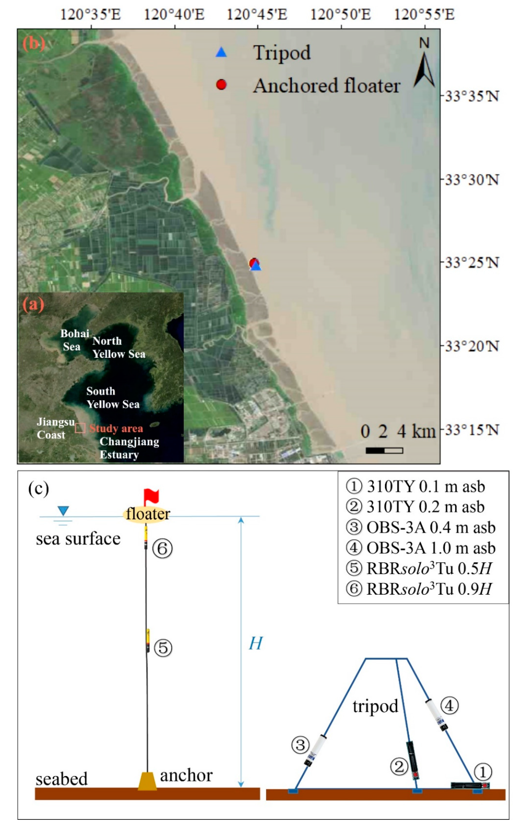
The middle of the Jiangsu coast, China, is characterized by high SSC (>1 kg/m³) [14], which makes it an excellent area to study the effectiveness, feasibility, and prospect of the above three types of optical turbidimeters in the in situ measurement of SSC of high-turbidity waters. A tripod was set on the inner shelf of the Dafeng Harbor on the middle of the Jiangsu coast during 12–14 November 2019 (Figure 1). The mean water depth of the observation site was around 7 m. Two 310TYs (0.1 and 0.2 m above the seabed (asb)) and two OBS-3As (0.4 and 1.0 m asb) were mounted on the tripod. A floater was anchored very close to the tripod, and two RBRsolo³Tu turbidimeters were deployed at the middle (0.5H, H denotes the water depth) and near-surface (0.9H) of the water column. These six instruments were all set to have a sampling frequency of 1 Hz, measuring for 30 s in each sampling interval of 3 min.

During the observation, 200 L water samples were taken from the middle layer of the water column at the site of the tripod. Meanwhile, 1 L water samples were collected from the layers near-surface and near-bottom, respectively. To ensure that sufficient sediments were collected, the samples were always taken at the flood/ebb maximum.

The above six turbidity sensors were calibrated in the laboratory. The seawater and suspended sediments collected from the middle layer of the water column were mixed into the lab samples of different SSCs (0.04–31.54 kg/m³), which were kept uniform by continuous stirring. Each turbidimeter was immersed in a lab sample (at the same height of 15 cm above the tank bottom) to obtain a steady output of turbidity and a sub-sample of 100 mL was taken to be filtered, dried off, and weighed to derive the SSC. The detailed procedure can be found in Shao and Maa (2017) [13].

The grain size distributions of suspended sediment in the water samples were measured using a laser diffraction particle size analyzer, the Malvern Mastersizer 2000. For suspended sediment in the middle layer, 3 sub-samples were taken from the well-mixed lab sample. The median grain size (D₅₀) and the mass contents of clay (<4 μm), silt (4~62.5 μm), and sand (>62.5 μm) of the sub-samples were thus obtained. Similarly, the grain size distributions were analyzed of the samples of the suspended sediment near-surface and near-bottom, as well as those of the surface bed sediment.

3. Results

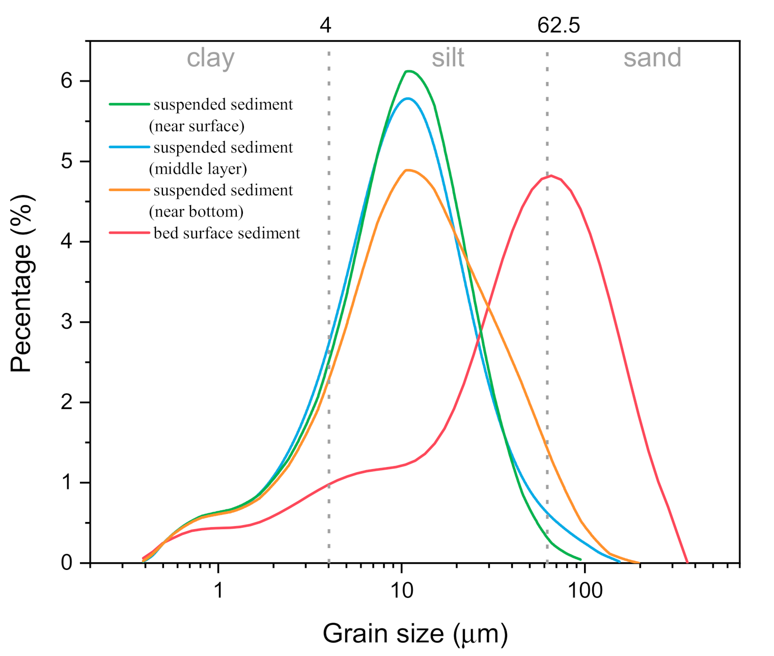
The grain-size distributions of the suspended sediments in the three sub-samples taken from the middle water column show few discrepancies and thus one of them was selected as a representative. D₅₀ of the suspended sediment was 9.3 μm, and clay (<4 μm), silt (4~62.5 μm), and sand (>62.5 μm) contents were 18.6%, 79.3%, and 2.1%, respectively, revealing the attributes of cohesive sediments [19]. Besides this, D₅₀ of the near-surface and near-bottom samples of suspended sediment was 9.4 μm and 11.1 μm. Clay, silt, and sand contents were 18.0%, 81.5%, and 0.5% for the near-surface sample and 16.7%, 78.9%, and 4.4% for the near-bottom sample. Thus, the grain-size distribution of the suspended sediment varied a little throughout the water column. The surface bed sediment was much coarser than the suspended sediment (Figure 2), the samples having a D₅₀ of 45.4 μm and contents of clay, silt, and sand of 10.0%, 49.8%, and 40.2%, respectively.

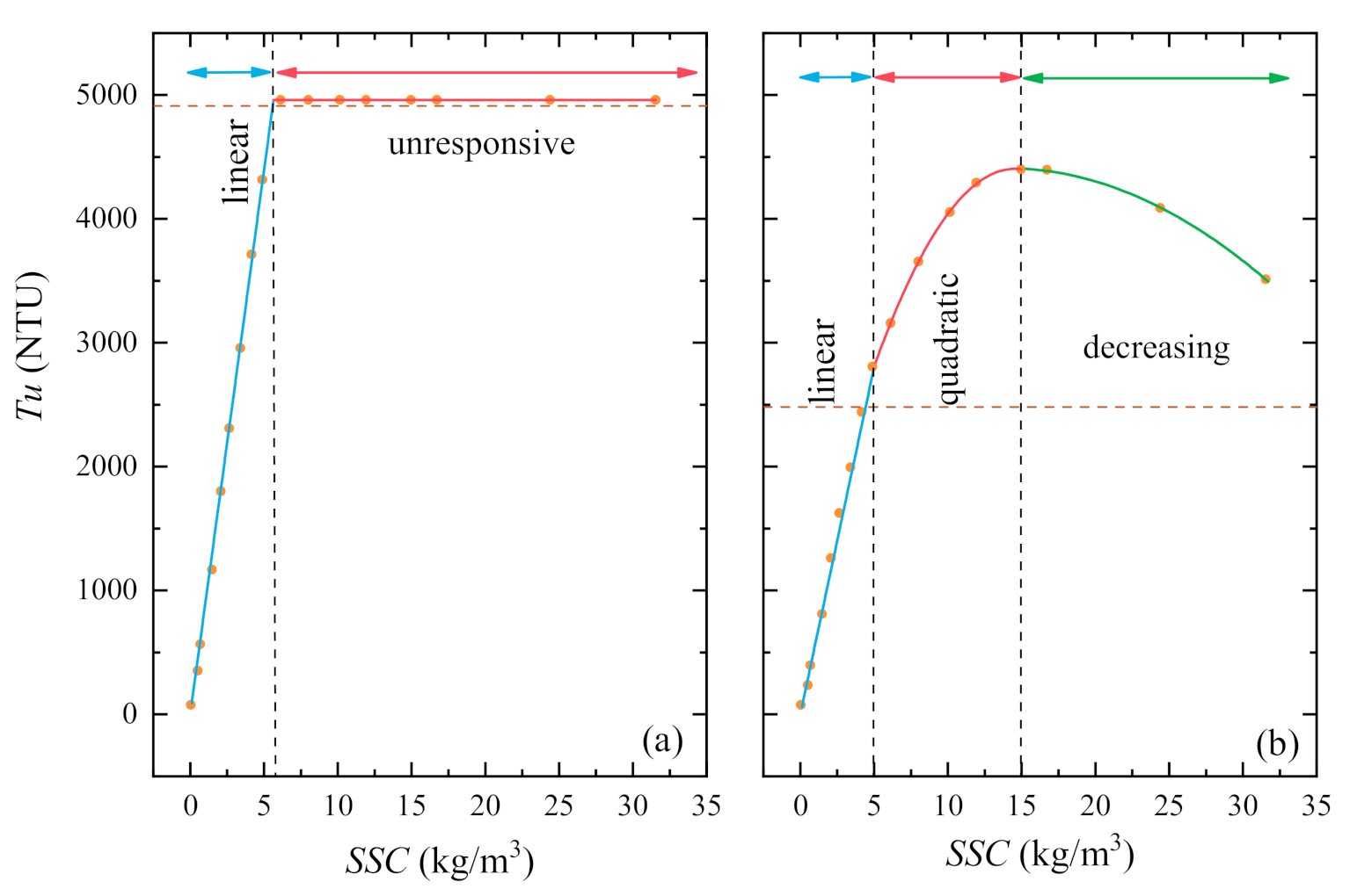
Each of the three types of turbidimeters had its patterns of calibration curves. Firstly, the conversions from Tu measured by the two OBS-3As to SSC were different (Figure 3). For the OBS-3A 0.4 m asb, the responses of Tu to SSC were divided into two SSC ranges: (1) low, 0 to 5.65 kg/m³, where the increase in Tu was approximately linear; (2) high, >5.65 kg/m³, where the curve was flat, suggesting the OBS-3A sensor was unresponsive to SSC changes. The response curves were initially fitted into various forms, including linear, second or third-order polynomials, exponential, logarithmic, and power laws. To make the curves as continuous as possible, some adjustments of coefficients were carried out to match the transition from one range to the next [11]. Two curving segments were chosen after a process of trial and error:

Tu = 877.59 C   (C < 5.65 kg/m³, R² = 0.99),

(1)

Tu = 4959.6   (C ≥ 5.65 kg/m³, R² = 1),

(2)

where Tu is turbidity in NTU and C is SSC in kg/m³. Equations (1) and (2) correspond to the linear and unresponsive ranges in Figure 3a.

However, for the OBS-3A 1.0 m asb, the data fell into three SSC ranges: (1) low, 0 to 4.95 kg/m³, turbidity approximately increased linearly; (2) mid, 4.95 to 14.95 kg/m³, the increase in turbidity tended to flatten, and a quadratic function applied to the fitting; (3) high, ≥14.95 kg/m³, where turbidity decreased with SSC. Finally, three sections of curves were confirmed:

Tu = 560.61 C    (C < 4.95 kg/m³, R² = 0.99),

(3)

Tu = −17.45 C² + 508.50 C + 700.44   (4.95 ≤ C < 14.95 kg/m³, R² = 0.99),

(4)

Tu = −2.89 C² + 80.43 C + 3850.30   (C ≥ 14.95 kg/m³, R² = 0.99),

(5)

Equations (3)–(5) denote the linear, quadratic, and decreasing ranges in Figure 3b.

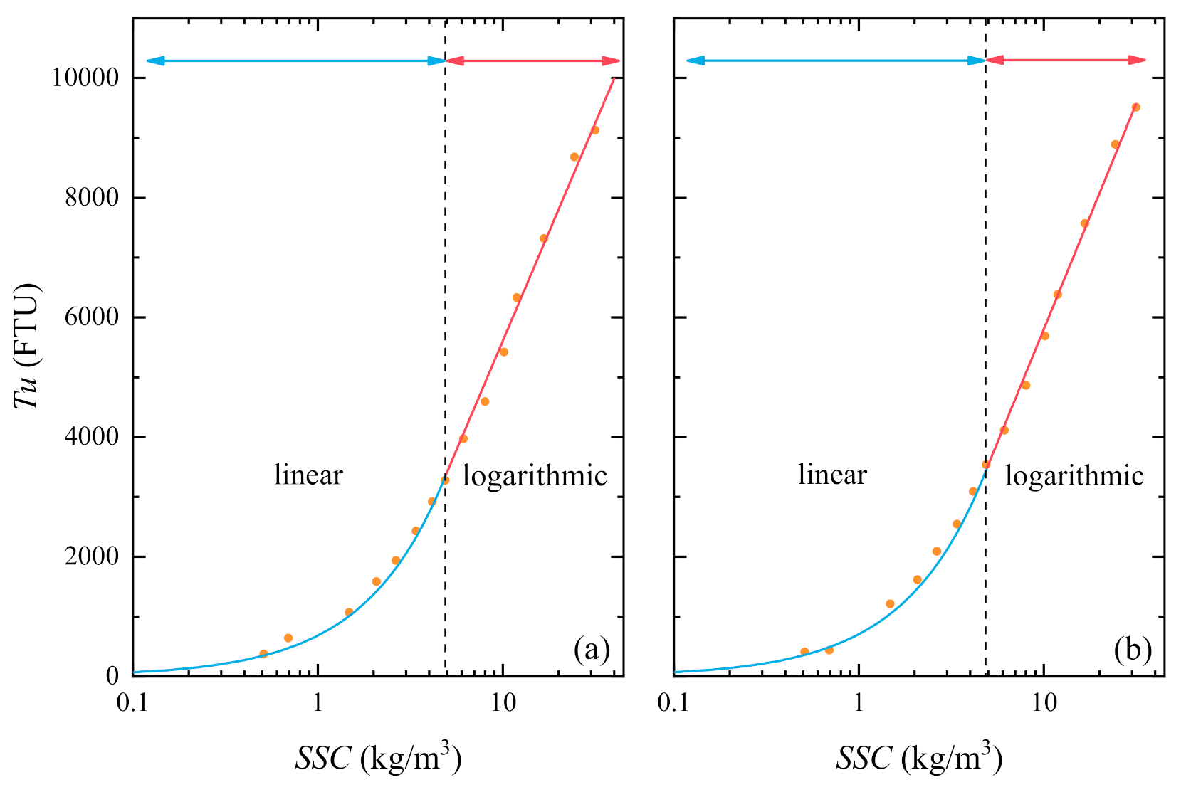
Secondly, the turbidity outputs of the two 310TYs 0.1 and 0.2 m asb responded coincidentally to the SSC of the lab samples. Both can be divided into two parts: (1) SSC was 0 to 4.88 kg/m³, water turbidity almost increased linearly with SSC; and (2) when SSC was larger than 4.88 kg/m³, turbidity increased with SSC in terms of logarithmic functions (Figure 4).

Equations (6) and (7) show the linear and logarithmic relations of the 310TY 0.1 m asb (Figure 4a), and those of the 310TY 0.2 m asb are expressed as in Equations (8) and (9) (Figure 4b).

Tu = 684.9 C   (C < 4.88 kg/m³, R² = 0.99),

(6)

Tu = 3160.8 lnC − 1668.2   (C ≥ 4.88 kg/m³, R² = 0.99),

(7)

Tu = 707.1 C   (C < 4.88 kg/m³, R² = 0.99),

(8)

Tu = 3277.8 lnC − 1745.9   (C ≥ 4.88 kg/m³, R² = 0.99),

(9)

in which Tu is turbidity in NTU and C is SSC in kg/m³.

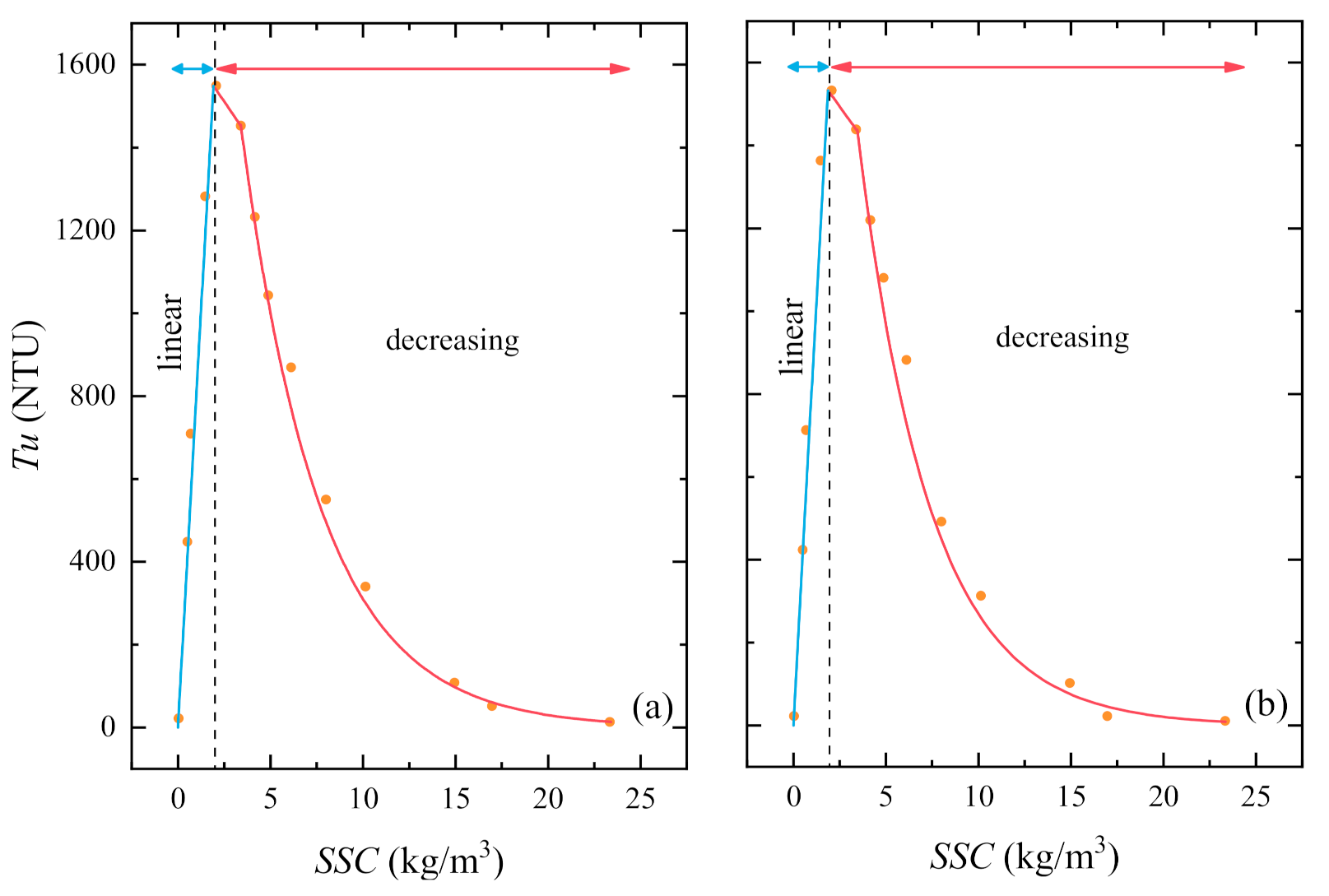
Thirdly, turbidity measured by the RBRsolo³Tu at 0.5H asb showed a consistent response to SSC with that of the RBRsolo³Tu at 0.9H asb. The calibration curves consist of two parts: (1) SSC < ca. 1.9 kg/m³, Tu increased linearly with SSC; and (2) SSC > ca. 1.9 kg/m³, Tu decreased with SSC (Figure 5).

For the RBRsolo³Tu at 0.5H asb, Equations (10)–(12) were determined to reflect the three sections of the response curve (Figure 5a):

Tu = 806.29 C   (C < 1.92 kg/m³, R² = 0.97),

(10)

Tu = −65.42 C + 1674.7   (1.92 ≤ C < 3.40 kg/m³, R² = 1),

(11)

Tu = 3223.2 e^{−0.234 C}   (C ≥ 3.40 kg/m³, R² = 0.99),

(12)

Likewise, Equations (13)–(15) denote the three sections for the RBRsolo³Tu at 0.9H asb, the first of which is linearly increasing and the others are decreasing in linear and exponential forms, respectively (Figure 5b):

Tu = 816.91 C   (C < 1.88 kg/m³, R² = 0.95),

(13)

Tu = −62.11 C + 1649.6   (1.88 ≤ C < 3.46 kg/m³, R² = 1),

(14)

Tu = 3487.3 e^{−0.256 C}   (C ≥ 3.46 kg/m³, R² = 0.97),

(15)

For the continuity of the calibration curves, the responsive data were fitted into three sections (Equations (10)–(15)). However, it was noted that the two-point regressions in Equations (11) and (14) may lead to errors and thus should be adopted with caution.

4. Discussion

4.1. Applications of the Calibration Curves

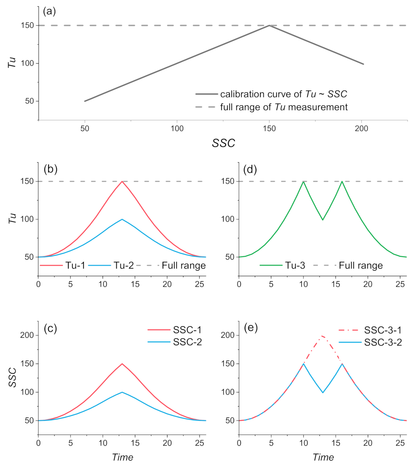
The purpose of the calibrations of the turbidity sensors is to obtain the SSC data from in situ measurements. Due to the existence of nonmonotonic Tu~SSC relationships, a challenge arises to identify which side of the calibration curves should be used, increasing turbidity output (low SSC) or decreasing turbidity output (high SSC) (e.g., Figure 3b and Figure 5). The use of observed time series can solve this problem to some extent, which can be understood through a diagram of Tu~SSC conversions (Figure 6).

Firstly, a calibration curve of Tu~SSC conversion is assumed as in Figure 6a. For turbidities from a small value to the maximum of the measuring range (i.e., the inflection point), the curvilinear sections showing positive responses of turbidity to SSC are applicable with no doubt. However, multi-solution is inevitable if the output of turbidity decreases after reaching the full range of measurements. This is likely due to the decrease or increase in SSC. The latter is associated with the turbidity increasing again to the full range after a high SSC event. Therefore, if only one peak exists in the time series of turbidity (Figure 6b), the curves can be applied with a positive response of turbidity to SSC (Figure 6c). Otherwise, if multiple peaks reach the full range of turbidity (Figure 6d), it is difficult to determine that SSC firstly increases and then decreases between two peaks or decreases first and then increases (Figure 6e).

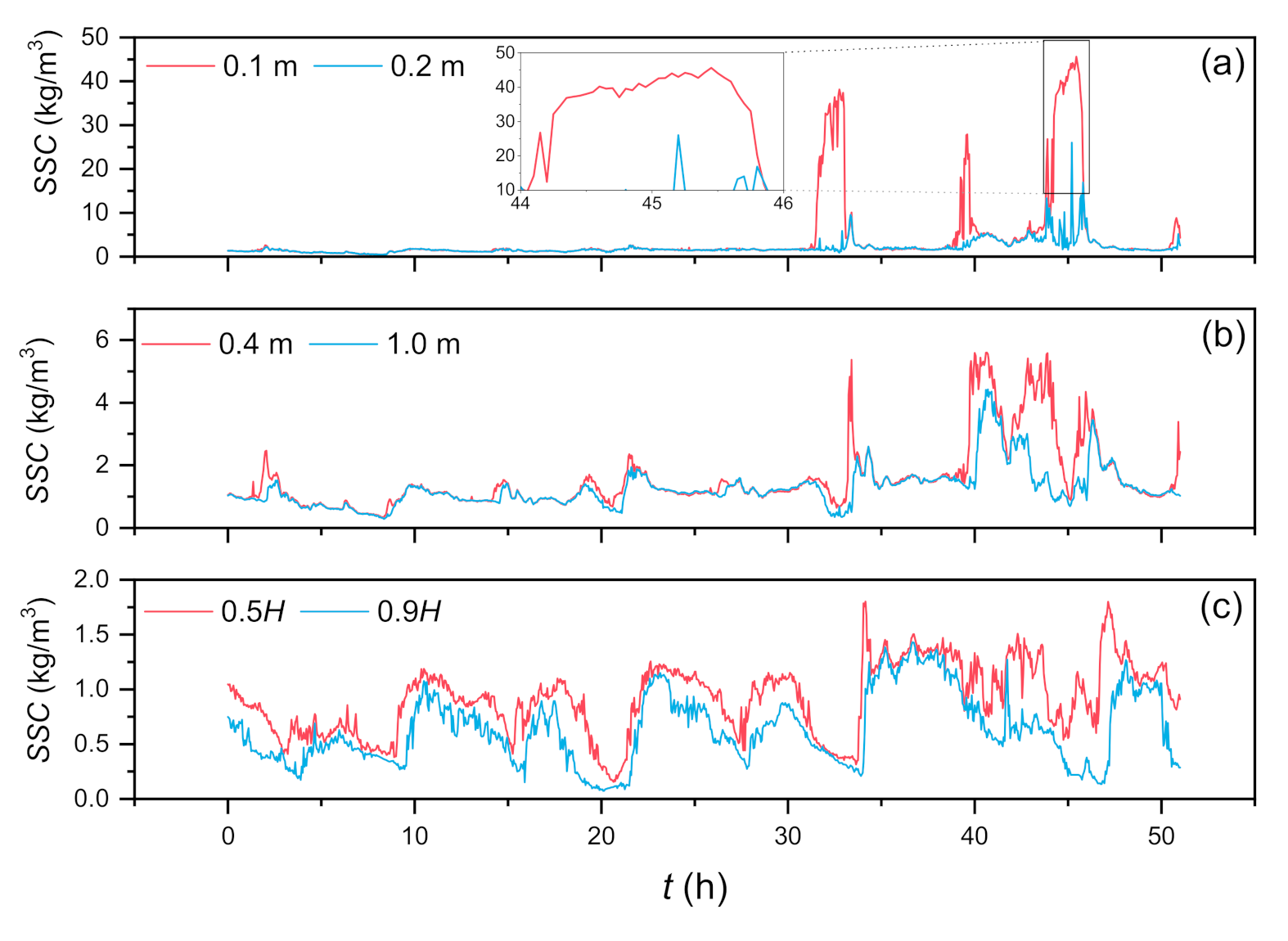
According to the above principles, the time series of turbidity at a variety of depths observed from the middle of the Jiangsu coast can be converted to those of SSC (Figure 7). Because the turbidity measured by 310TY monotonically responds to SSC (Figure 4) and only a peak occurs in the time series of turbidity at 0.1 and 0.2 m asb, these turbidities can be converted to SSC using Equations (6)–(9). Figure 7a reveals that three fluid-mud events take place near the seabed (t = 31.55~33.05 h, 39.45~39.7 h, and 43.8~45.85 h), during which the thickness of fluid-mud is larger than 10 cm and SSC > 10 kg/m³ [16].

The maximum turbidities measured by OBS-3A at 0.4 and 1.0 m asb are 4912.2 and 2480.9 NTU, and both are smaller than the upper limits of the linear ranges, i.e., 4959.6 and 2755.0 NTU (Figure 3). Equations (1) and (3) can thus be applied to derive the SSC 0.4 and 1.0 m asb (Figure 7b), the peak SSCs attaining 5.60 and 4.43 kg/m³, respectively. In the same way, the full ranges of turbidity observed by RBRsolo³Tu at 0.5H and 0.9H asb are included in those of the linear ranges of the calibration curves (Figure 5). Therefore, the time series of SSC are calculated using Equations (10) and (13), with peak SSCs of 1.80 and 1.43 kg/m³, respectively (Figure 7c).

4.2. Comparisons with Previous Studies

Although studies on the calibrations of 310TY and RBRsolo³Tu have been rarely reported, the results of OBS-3A calibrations in this study are comparable with previous research. Kineke and Sternberg calibrated the OBS at the Amazon estuary [11] and so did Shao and Maa at the Changjiang estuary [13]. The overall patterns of their calibration curves are the same as in this study: (1) at low SSCs, the OBS output increases approximately linearly with SSC; (2) as SSC continues to increase, the growth of the OBS output slows down until an inflection point is reached, and this section of the curve can be fitted as a quadratic function; and (3) for larger SSCs, the OBS output is decreasing. The linear ranges and the inflection points vary slightly: the former is 0~10 kg/m³ [11] and 0~5 kg/m³ [13] in the previous research and 0~4.95 kg/m³ for the OBS-3A at 1.0 m asb here; and the latter is 19 kg/m³ [11], ca. 15 kg/m³ [13], and 14.95 kg/m³ in this study. These differences can be attributed to distributions of suspended sediment grain/floc size [10].

The different patterns of the calibration curves for the two OBS-3As at 0.4 and 1.0 m asb are dependent on the gain setting [11]. The OBS-3A at 0.4 m asb is associated with the high set of gain (i.e., Tu is more sensitive to smaller SSC changes), which leads to the turbidity output initially increasing linearly to the full range as SSC increases and then remains at the full range (Figure 3a) until SSC is sufficiently high to cause a decrease in turbidity [11]. By contrast, if the gain is set low to match the maximum turbidity output (the inflection point), the case of the OBS-3A at 1.0 m asb takes place (Figure 3b).

4.3. Comparison of the Performance of the Three Instruments

The full ranges of turbidity measured by OBS-3A and RBRsolo³Tu are around 4500 and 1600 NTU, respectively, which correspond to the inflection points of the calibration curves. On either side of the inflection point, Tu is positively (left) or negatively (right) correlated to SSC. A given turbidity output is likely to correspond to two SSC values which are smaller or larger than that of the inflection point. This gives rise to difficulties in the conversion of Tu~SSC when the maximum Tu reaches the full range several times (Figure 6d,e). Therefore, the use of OBS-3A or RBRsolo³Tu in continuous measurement of SSC at a fixed point is only appropriate for SSCs smaller than the inflection point (ca. 15 kg/m³ for OBS-3A and 2 kg/m³ for RBRsolo³Tu in this study). It is found that a positive correlation of Tu~SSC occurs under SSC < ca. 40 kg/m³ for the identical sediment if using the 310TY with a full range up to ca. 10,000 FTU. Thus, 310TY has important prospects for field applications in high-SSC environments.

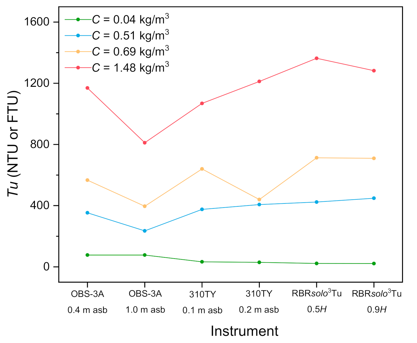
The six turbidimeters respond differently to an identical SSC, e.g., 0.04, 0.51, 0.69, and 1.48 kg/m³ (Figure 8). All these SSCs are within the linear ranges and in response to a certain SSC, the outputs of the three types of turbidity sensors differentiate from each other. Besides this, due to different gain settings, the responses of turbidimeters are dissimilar even if they have the same type of sensor. Assuming that 1 NTU equals 1 FTU, in response to an SSC of 1.48 kg/m³, for example, the differences in the outputs of the six turbidimeters range from 42.6 to 552.6 NTU, which accounts for 3.7~48.0% of the average. Moreover, the outputs at SSC = 1.48 kg/m³ from the two OBS-3A sensors vary up to 358.4 NTU, which is 36.2% of their average.

It is noted that grain-size distribution, flocculation of fine particles, and sediment mineralogy greatly influence the Tu~SSC calibration curves [6,10,20,21,22,23,24]. The surface bed sediment is much coarser than the suspended sediment here (Figure 2), and SSC would be excessively overestimated if using the surface bed sediment for calibrations [6,20,21,22]. Therefore, it is a prerequisite to use the suspended sediment in the water samples when calibrating SSCs. Moreover, there is a hypothesis that the grain-size distribution, flocculation of fine particles, and sediment mineralogy remain stable during the field measurement and are identical to those of the suspended sediment in the lab samples for calibration. On such a basis, the Tu~SSC calibration curves can be applied to obtain the time series of the in situ SSC. This issue deserves further study in the future.

5. Conclusions

Three optical instruments (OBS-3A, 310TY, and RBRsolo³Tu with Seapoint sensor) were deployed in the in situ measurement of turbidity at the middle of the Jiangsu coast, China, and water and suspended sediment samples collected from the observation site were used in the lab calibrations of these three instruments. The calibration curves can be built showing the relationships between turbidity and SSC, with the range of observed SSC up to 31.5 kg/m³. The results show that both the calibration curves of OBS-3A and RBRsolo³Tu have an inflection point (at SSC of ca. 15 kg/m³ for OBS-3A and ca. 2 kg/m³ for RBRsolo³Tu), on either side of which turbidity increases (the left side) or decreases (the right side) with the increasing SSC. Only under SSCs smaller than the inflection point can OBS-3A and RBRsolo³Tu be applied to continuous SSC measurements at a fixed point. However, the turbidity output of 310TY has always a positive correlation with SSC, which applies for SSC up to 40 kg/m³; thus, three fluid-mud events are quantified during this observation. In conclusion, 310TY has important prospects for field applications in high-SSC environments.

References

- Nittrouer, C.A.; Austin, J.A., Jr.; Field, M.E.; Kravitz, J.H.; Syvitski, J.P.M.; Wiberg, P.L. Writing a Rosetta Stone: Insights into Continental-Margin Sedimentary Processes and Strata. In Continental Margin Sedimentation; Nittrouer, C.A., Austin, J.A., Field, M.E., Kravitz, J.H., Syvitski, J.P.M., Wiberg, P.L., Eds.; Wiley: Hoboken, NJ, USA, 2007; pp. 1–48. [Google Scholar] [CrossRef]
- Eidam, E.F.; Ogston, A.S.; Nittrouer, C.A. Formation and removal of a coastal flood deposit. J. Geophys. Res. Ocean. 2019, 124, 1045–1062. [Google Scholar] [CrossRef]
- Becker, M.; Maushake, C.; Winter, C. Observations of mud-induced periodic stratification in a hyperturbid estuary. Geophys. Res. Lett. 2018, 45, 5461–5469. [Google Scholar] [CrossRef]
- Venkatesan, M.I.; Merino, O.; Baek, J.; Northrup, T.; Sheng, Y.; Shisko, J. Trace organic contaminants and their sources in surface sediments of Santa Monica Bay, California, USA. Mar. Environ. Res. 2010, 69, 350–362. [Google Scholar] [CrossRef] [PubMed] [Green Version]
- Dethier, E.N.; Renshaw, C.E.; Magilligan, F.J. Toward improved accuracy of remote sensing approaches for quantifying suspended sediment: Implications for suspended-sediment monitoring. J. Geophys. Res. Earth Surf. 2020, 125, e2019JF005033. [Google Scholar] [CrossRef]
- Downing, J. Twenty-five years with OBS sensors: The good, the bad, and the ugly. Cont. Shelf Res. 2006, 26, 2299–2318. [Google Scholar] [CrossRef]
- Wang, A.; Ye, X.; Du, X.; Zheng, B. Observations of cohesive sediment behaviors in the muddy area of the northern Taiwan Strait, China. Cont. Shelf Res. 2014, 90, 60–69. [Google Scholar] [CrossRef]
- Weiss, A.; Clark, S.P.; Rennie, C.D.; Moore, S.A.; Ahmari, H. Estimation of total suspended solids concentration from aDcp backscatter and hydraulic measurements. J. Hydraul. Res. 2015, 53, 670–677. [Google Scholar] [CrossRef]
- Fettweis, M.; Riethmüller, R.; Verney, R.; Becker, M.; Backers, J.; Baeye, M.; Chapalain, M.; Claeys, S.; Claus, J.; Cox, T.; et al. Uncertainties associated with in situ high-frequency long-term observations of suspended particulate matter concentration using optical and acoustic sensors. Prog. Oceanogr. 2019, 178, 102162. [Google Scholar] [CrossRef]
- Maa, J.P.Y.; Xu, J.; Victor, M. Notes on the performance of an optical backscatter sensor for cohesive sediments. Mar. Geol. 1992, 104, 215–218. [Google Scholar] [CrossRef]
- Kineke, G.C.; Sternberg, R.W. Measurements of high concentration suspended sediments using the optical backscatterance sensor. Mar. Geol. 1992, 108, 253–258. [Google Scholar] [CrossRef]
- Sutherland, T.F.; Lane, P.M.; Amos, C.L.; Downing, J. The calibration of optical backscatter sensors for suspended sediment of varying darkness levels. Mar. Geol. 2000, 162, 587–597. [Google Scholar] [CrossRef]
- Shao, Y.; Maa, J.P.-Y. Comparisons of different instruments for measuring suspended cohesive sediment concentrations. Water 2017, 9, 968. [Google Scholar] [CrossRef] [Green Version]
- Yu, Q.; Wang, Y.; Shi, B.; Wang, Y.P.; Gao, S. Physical and sedimentary processes on the tidal flat of central Jiangsu Coast, China: Headland induced tidal eddies and benthic fluid mud layers. Cont. Shelf Res. 2017, 133, 26–36. [Google Scholar] [CrossRef]
- Rymszewicz, A.; O’Sullivan, J.J.; Bruen, M.; Turner, J.N.; Lawler, D.M.; Conroy, E.; Kelly-Quinn, M. Measurement differences between turbidity instruments, and their implications for suspended sediment concentration and load calculations: A sensor inter-comparison study. J. Environ. Manag. 2017, 199, 99–108. [Google Scholar] [CrossRef]
- Wright, L.D.; Friedrichs, C.T. Gravity-driven sediment transport on continental shelves: A status report. Cont. Shelf Res. 2006, 26, 2092–2107. [Google Scholar] [CrossRef]
- Liu, J.T.; Wang, Y.-H.; Yang, R.J.; Hsu, R.T.; Kao, S.-J.; Lin, H.-L.; Kuo, F.H. Cyclone-induced hyperpycnal turbidity currents in a submarine canyon. J. Geophys. Res. Ocean. 2012, 117, C04033. [Google Scholar] [CrossRef]
- Baek, Y.S.; Chun, S.S.; Chang, T.S.; Kim, J.K. The role of fluid mud in the formation of extensive mud sheets during summer on the Duuri macrotidal flat, west coast of Korea. Geosci. J. 2018, 22, 19–32. [Google Scholar] [CrossRef]
- van Rijn, L.C. Unified View of Sediment Transport by Currents and Waves. I: Initiation of Motion, Bed Roughness, and Bed-Load Transport. J. Hydraul. Eng. 2007, 133, 649–667. [Google Scholar] [CrossRef] [Green Version]
- Xu, J.P. Converting near-bottom OBS measurements into suspended sediment concentrations. Geo-Mar. Lett. 1997, 17, 154–161. [Google Scholar] [CrossRef]
- Bunt, J.A.C.; Larcombe, P.; Jago, C.F. Quantifying the response of optical backscatter devices and transmissometers to variations in suspended particulate matter. Cont. Shelf Res. 1999, 19, 1199–1220. [Google Scholar] [CrossRef]
- Landers, M.N.; Sturm, T.W. Hysteresis in suspended sediment to turbidity relations due to changing particle size distributions. Water Resour. Res. 2013, 49, 5487–5500. [Google Scholar] [CrossRef]
- Druine, F.; Verney, R.; Deloffre, J.; Lemoine, J.-P.; Chapalain, M.; Landemaine, V.; Lafite, R. In situ high frequency long term measurements of suspended sediment concentration in turbid estuarine system (Seine Estuary, France): Optical turbidity sensors response to suspended sediment characteristics. Mar. Geol. 2018, 400, 24–37. [Google Scholar] [CrossRef] [Green Version]
- River, M.; Richardson, C.J. Suspended sediment mineralogy and the nature of suspended sediment particles in stormflow of the southern piedmont of the USA. Water Resour. Res. 2019, 55, 5665–5678. [Google Scholar] [CrossRef]
Figure 1.
Maps of the study area: (a) regional overview. The red rectangle denotes the study area; (b) observation sites. The triangle and circle represent the tripod and the anchored floater, respectively; (c) scheme of the vertical deployment of the instruments.
Figure 2.
Grain-size distributions of the samples of suspended sediment (curves in green, blue, and orange) and bed surface sediment (red curve). The dotted lines mark the grain-size range of silt (4~62.5 μm).
Figure 3.
Laboratory calibration for OBS-3A on the tripod showing the response of Tu to SSC of the lab samples: (a) 0.4 m asb; (b) 1.0 m asb. The dashed horizontal lines mark the maximum values of the measured turbidity.
Figure 4.
Laboratory calibration for 310TY on the tripod showing the response of Tu to SSC of the lab samples: (a) 0.1m asb; (b) 0.2 m asb.
Figure 5.
Laboratory calibration for RBRsolo3Tu bonded to the anchored floater showing the response of Tu to SSC of the lab samples: (a) 0.5H asb; (b) 0.9H asb. H is the water depth.
Figure 6.
Diagram of Tu~SSC conversions: (a) Schematized Tu~SSC calibration curve and the full range of Tu measurement is marked; (b) Tu-1 and Tu-2: two types of temporal variations of Tu both having only one peak (≤full range); (c) SSC-1 and SSC-2: temporal variations of SSC converted from Tu-1 and Tu-2 by the left (monotonic increasing) side of the calibration curve in subplot (a), respectively; (d) Tu-3: the third type temporal variations of Tu, showing two peaks at the full range of Tu measurement; (e) SSC-3-1 and SSC-3-2: possible SSC time series corresponding to Tu-3, in which SSC-3-1 indicates that SSC firstly increases and then decreases between the two peaks of Tu-3 while SSC-3-2 is the opposite. Note that the values in the coordinates only denote relative magnitudes.
Figure 7.
Time series of the in situ SSC measured at the middle of the Jiangsu coast, China, by the three types of turbidimeters (310TY, OBS-3A, and RBRsolo3Tu), starting from 09:30 November 12, 2019. The mean water depth of the observation site is around 7 m.
Figure 8.
Outputs from the six turbidimeters in response to an identical SSC (0.04, 0.51, 0.69, and 1.48 kg/m3).
Publisher’s Note: MDPI stays neutral with regard to jurisdictional claims in published maps and institutional affiliations. |
© 2020 by the authors. Licensee MDPI, Basel, Switzerland. This article is an open access article distributed under the terms and conditions of the Creative Commons Attribution (CC BY) license (http://creativecommons.org/licenses/by/4.0/).
Share and Cite
MDPI and ACS Style
Wang, Y.; Peng, Y.; Du, Z.; Lin, H.; Yu, Q. Calibrations of Suspended Sediment Concentrations in High-Turbidity Waters Using Different In Situ Optical Instruments. Water 2020, 12, 3296. https://doi.org/10.3390/w12113296
AMA Style
Wang Y, Peng Y, Du Z, Lin H, Yu Q. Calibrations of Suspended Sediment Concentrations in High-Turbidity Waters Using Different In Situ Optical Instruments. Water. 2020; 12(11):3296. https://doi.org/10.3390/w12113296
Chicago/Turabian StyleWang, Yunwei, Yun Peng, Zhiyun Du, Hangjie Lin, and Qian Yu. 2020. "Calibrations of Suspended Sediment Concentrations in High-Turbidity Waters Using Different In Situ Optical Instruments" Water 12, no. 11: 3296. https://doi.org/10.3390/w12113296
Note that from the first issue of 2016, this journal uses article numbers instead of page numbers. See further details here.