the Creative Commons Attribution 4.0 License.
the Creative Commons Attribution 4.0 License.
 | 23 Nov 2020
Exploring constraints on a wetland methane emission ensemble (WetCHARTs) using GOSAT observations
Chris Wilson
A. Anthony Bloom
Edward Comyn-Platt
Garry Hayman
Joe McNorton
Hartmut Boesch
Martyn P. Chipperfield
Wetland emissions contribute the largest uncertainties to the current global atmospheric CH4 budget, and how these emissions will change under future climate scenarios is also still poorly understood. Bloom et al. (2017b) developed WetCHARTs, a simple, data-driven, ensemble-based model that produces estimates of CH4 wetland emissions constrained by observations of precipitation and temperature. This study performs the first detailed global and regional evaluation of the WetCHARTs CH4 emission model ensemble against 9 years of high-quality, validated atmospheric CH4 observations from GOSAT (the Greenhouse Gases Observing Satellite). A 3-D chemical transport model is used to estimate atmospheric CH4 mixing ratios based on the WetCHARTs emissions and other sources.
Across all years and all ensemble members, the observed global seasonal-cycle amplitude is typically underestimated by WetCHARTs by −7.4 ppb, but the correlation coefficient of 0.83 shows that the seasonality is well-produced at a global scale. The Southern Hemisphere has less of a bias (−1.9 ppb) than the Northern Hemisphere (−9.3 ppb), and our findings show that it is typically the North Tropics where this bias is the worst (−11.9 ppb).
We find that WetCHARTs generally performs well in reproducing the observed wetland CH4 seasonal cycle for the majority of wetland regions although, for some regions, regardless of the ensemble configuration, WetCHARTs does not reproduce the observed seasonal cycle well. In order to investigate this, we performed detailed analysis of some of the more challenging exemplar regions (Paraná River, Congo, Sudd and Yucatán). Our results show that certain ensemble members are more suited to specific regions, due to either deficiencies in the underlying data driving the model or complexities in representing the processes involved. In particular, incorrect definition of the wetland extent is found to be the most common reason for the discrepancy between the modelled and observed CH4 concentrations. The remaining driving data (i.e. heterotrophic respiration and temperature) are shown to also contribute to the mismatch with observations, with the details differing on a region-by-region basis but generally showing that some degree of temperature dependency is better than none.
We conclude that the data-driven approach used by WetCHARTs is well-suited to producing a benchmark ensemble dataset against which to evaluate more complex process-based land surface models that explicitly model the hydrological behaviour of these complex wetland regions.


The uncertainty in the emissions from natural wetlands remains the most significant uncertainty in the global CH4 budget (Melton et al., 2013; Kirschke et al., 2013; Saunois et al., 2020). Without a more complete understanding of the processes by which wetlands emit CH4 and, more importantly, how sensitive these processes are to changes in different driving factors such as precipitation, respiration and temperature, any attempt to model global CH4 emissions for future climate change scenarios remains challenging and prone to large uncertainties (Z. Zhang et al., 2017; Ganesan et al., 2019). Previous studies (Bohn et al., 2015; Poulter et al., 2017) have suggested that it is the uncertainty around wetland extent that is the largest contributor to uncertainties in the total methane emissions, with uncertainties in the climate response driving the interannual variability.
It is acknowledged (Kleinen et al., 2012; Stocker et al., 2014) that we currently lack sufficient observations to fully constrain estimates of wetland extent produced via land surface process models and that such differences in modelled wetland extent can account for an uncertainty of between 30 % and 40 % in the global wetland CH4 emission estimates (Saunois et al., 2016). Recent work by Tootchi et al. (2019) provides an excellent summary of the current literature and highlights the differences between the multitude of wetland extent datasets currently in use. Furthermore, our previous work (Parker et al., 2018) has shown that important processes such as river overbank inundation can contribute significantly to wetland CH4 emissions but such processes are often lacking in models and, due to their infrequent nature, are not always represented in wetland extent maps.
Given the consensus that there is currently a lack of observations sufficient to fully constrain the CH4 emissions from more complex land surface models, there is a clear opportunity for a simple, data-driven, ensemble-based model, such as WetCHARTs, that is capable of producing estimates of CH4 wetland emissions.
In this study we perform a thorough global and regional evaluation of the WetCHARTs CH4 wetland model ensemble using satellite observations of atmospheric CH4 from GOSAT (the Greenhouse Gases Observing Satellite) with the aim of
-
identifying whether WetCHARTs is capable of reproducing the observed wetland CH4 seasonal cycle at both the global and regional scale,
-
determining whether we can exploit the ensemble of WetCHARTs data to explain the cause of any discrepancies against observations,
-
improving our understanding of which drivers are the most important for constraining wetland CH4 emissions both spatially and temporally,
-
determining whether WetCHARTs can be used as a suitable benchmark against which to assess more complex process-based land surface models.
WetCHARTs (Bloom et al., 2017b) is a wetland CH4 emission dataset derived from satellite-based surface inundation extent and precipitation reanalyses, model-based heterotrophic respiration, and a range of temperature dependencies. WetCHARTs has been used in a range of studies (including Parker et al., 2018; Treat et al., 2018; Sheng et al., 2018; Lunt et al., 2019; Maasakkers et al., 2019) typically as the wetland CH4 a priori in global or regional flux inversion experiments. This study uses v1.2.1 of WetCHARTs which extends the ensemble to 2017. In addition to the extension in time, wetland extent across Lehner and Döll (2004) wetland complex classes 0 %–25 %, 25 %–50 % and 50 %–100 % were scaled by 12.5 %, 37.5 % and 75 % respectively.
Fundamentally, WetCHARTs works by calculating spatially (x) and temporally (t) resolved CH4 fluxes at a 0.5∘ × 0.5∘ resolution globally using the following equation:
where A(t,x) is the wetland extent fraction, itself given by , with w(x) being the static wetland extent fraction and h(t,x) being the temporal variability. R(t,x) is the heterotrophic carbon respiration per unit area. The term represents the temperature dependence of the CH4 : C ratio, with Q10 being the relative CH4 : C respiration for a 10 ∘C increase and T(t,x) being the surface skin temperature. s is a global scale factor. Many other studies and wetland emission models utilise some form of this equation to estimate methane wetland fluxes (Gedney et al., 2004; Eliseev et al., 2008; Clark et al., 2011; Xu et al., 2016; Poulter et al., 2017; Comyn-Platt et al., 2018).
Figure 1 shows the configurations of the WetCHARTs ensemble members used in this study and also provides guidance on the four-digit identification which will be used to describe the individual ensemble members from here on.
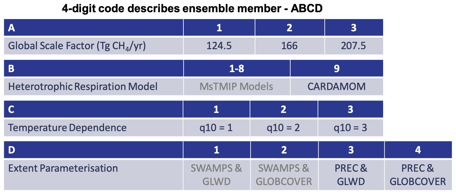
Figure 1Description of the four-digit code used throughout this work to identify the configuration of the WetCHARTs ensemble members. For the extended WetCHARTs period of 2009–2018, there is only one heterotrophic-respiration model (CARDAMOM) and two wetland extent parametrisations (using ERA-Interim precipitation) available, giving a total of 18 different configurations.
The global scale factor (s in Eq. 1) is a model-specific scaling factor (Bloom et al., 2017b), derived such that model annual emissions amount to 124.5, 166 or 207.5 Tg CH4 yr−1, which represent the mean 2000–2009 wetland emission estimates from Saunois et al. (2016) along with a ± 25 % uncertainty. The full ensemble (FE) utilises nine heterotrophic-respiration models for 2010 (Huntzinger et al., 2013), but the extended ensemble (EE) used here (2009–2017) is limited to the CARDAMOM data-constrained terrestrial carbon cycle analysis (Bloom et al., 2016) to calculate values for R. ERA-Interim skin temperature is used as the underlying temperature driving data, and the temperature dependence spans three values for Q10, ranging from 1 (i.e. no temperature dependence) to 3 (high temperature dependence). Finally, the wetland extent parametrisation (A) for the extended ensemble uses normalised monthly mean ERA-Interim precipitation (Dee et al., 2011) with a static wetland map taken from either the Global Lakes and Wetlands Database (GLWD – Lehner and Döll, 2004) or GlobCover (Bontemps et al., 2011) to give spatially and temporally varying wetland extent.
In total, for the extended ensemble covering 2009–2017, the above criteria result in 18 ensemble members (3×s, 1×R, 3×Q10, 2×A). For more extensive details on the ensemble members see Bloom et al. (2017b).
Throughout this study we refer to each ensemble member by a four-digit code (Fig. 1). For example, the ensemble member with a global scale factor of 166 Tg CH4 yr−1, using CARDAMOM for its heterotrophic respiration, with a temperature dependence of Q10=3 and using precipitation with the Global Lakes and Wetlands Database to define the extent would be identified as 2933. When referring to the parameter but not a specific configuration, the xxCx nomenclature is used (e.g. temperature dependency), and when referring to a specific value for a set of configurations, the xx1x nomenclature is used (e.g. all ensemble members with a Q10=1 temperature dependency).
In order to compare the CH4 emissions from WetCHARTs with atmospheric CH4 observations, we process the emissions through a global 3-D atmospheric chemistry transport model, TOMCAT (Chipperfield, 2006). Throughout this study, when we refer to CH4 concentrations from WetCHARTs, we are referring to the output from TOMCAT simulations using the WetCHARTs wetland emissions. These TOMCAT simulations are performed globally at a 1.125∘ horizontal resolution between 2009 and 2017 using ERA-Interim meteorology to force the model (Dee et al., 2011). The WetCHARTs ensemble is used as the surface wetland emissions. Each ensemble member from WetCHARTs, as described in Sect. 2, is used to simulate a separate CH4 tracer, along with a reference CH4 tracer that has all other CH4 emission sectors included apart from wetland emissions, resulting in 19 model tracer simulations. The non-wetland CH4 fluxes are kept consistent between all simulations, using EDGAR (v4.2; Olivier et al., 2012) for anthropogenic emissions and GFED (v4.1s; van der Werf et al., 2017) for biomass burning. The EDGARv4.2 database runs up to 2012, and we repeat the 2012 emissions for the remaining years, with no seasonal cycle applied. As we focus primarily on wetland emission areas, the local seasonal cycle due to anthropogenic fluxes is likely very small compared to natural sources. We do however note the possibility that this assumption could be a source of uncertainty. We used the GFEDv4.2 emissions for the correct year up to and including 2016 and used a climatology for 2017 and 2018.
Prescribed annually repeating values taken from Yan et al. (2009) are used for rice paddy emissions, with the remaining emissions (oceans, termites) used as described in Patra et al. (2011). The atmospheric sink is included via annually repeating atmospheric OH and O(1D) fields, and the methanotrophic-soil sink is included as in McNorton et al. (2016).
This study uses satellite observations of total column dry air mole fractions of CH4 (XCH4) generated by the University of Leicester Proxy XCH4 GOSAT retrieval (Parker et al., 2011, 2015, 2020) as part of the ESA Climate Change Initiative (Buchwitz et al., 2017) and the Copernicus Climate Change Service (Buchwitz et al., 2018).
The GOSAT XCH4 data have been extensively validated (Dils et al., 2014; Parker et al., 2015; Buchwitz et al., 2017; Parker et al., 2020), primarily using data from the Total Carbon Column Observing Network (TCCON). TCCON is a global network of ground-based, high-resolution Fourier transform spectrometers recording direct solar spectra in the near-infrared spectral region (Wunch et al., 2011). The TCCON data are tied to World Meteorological Organization (WMO) standards (Wunch et al., 2010) and are the primary validation data for satellite observations of greenhouse gases (Cogan et al., 2012; Wunch et al., 2011; Dils et al., 2014). After performing extensive validation on TCCON, we subtract one global offset from the GOSAT data. This value is typically small. For v7.2 of the data (as used in this study), the value was 7.71 ppb. For our latest data, v9.0, the value is 9.06 ppb (see Parker et al., 2020, under review)
This version of the GOSAT Proxy XCH4 data (v7.2) agrees well with TCCON data, with an overall bias of 0.32 ppb, a standard deviation of 13.64 ppb and a correlation coefficient of 0.91 between the 73 304 coincident GOSAT–TCCON measurements. GOSAT XCH4 has additionally been validated against aircraft measurements over the Amazon (Webb et al., 2016).
These data have been heavily utilised by the atmospheric inversion community, and many studies (Fraser et al., 2013; Cressot et al., 2014; Turner et al., 2016; Alexe et al., 2015; Berchet et al., 2015; Feng et al., 2017; Ganesan et al., 2017; Sheng et al., 2018; Maasakkers et al., 2019; Saunois et al., 2020; Lunt et al., 2019) have used these data to successfully infer regional and global emissions of CH4.
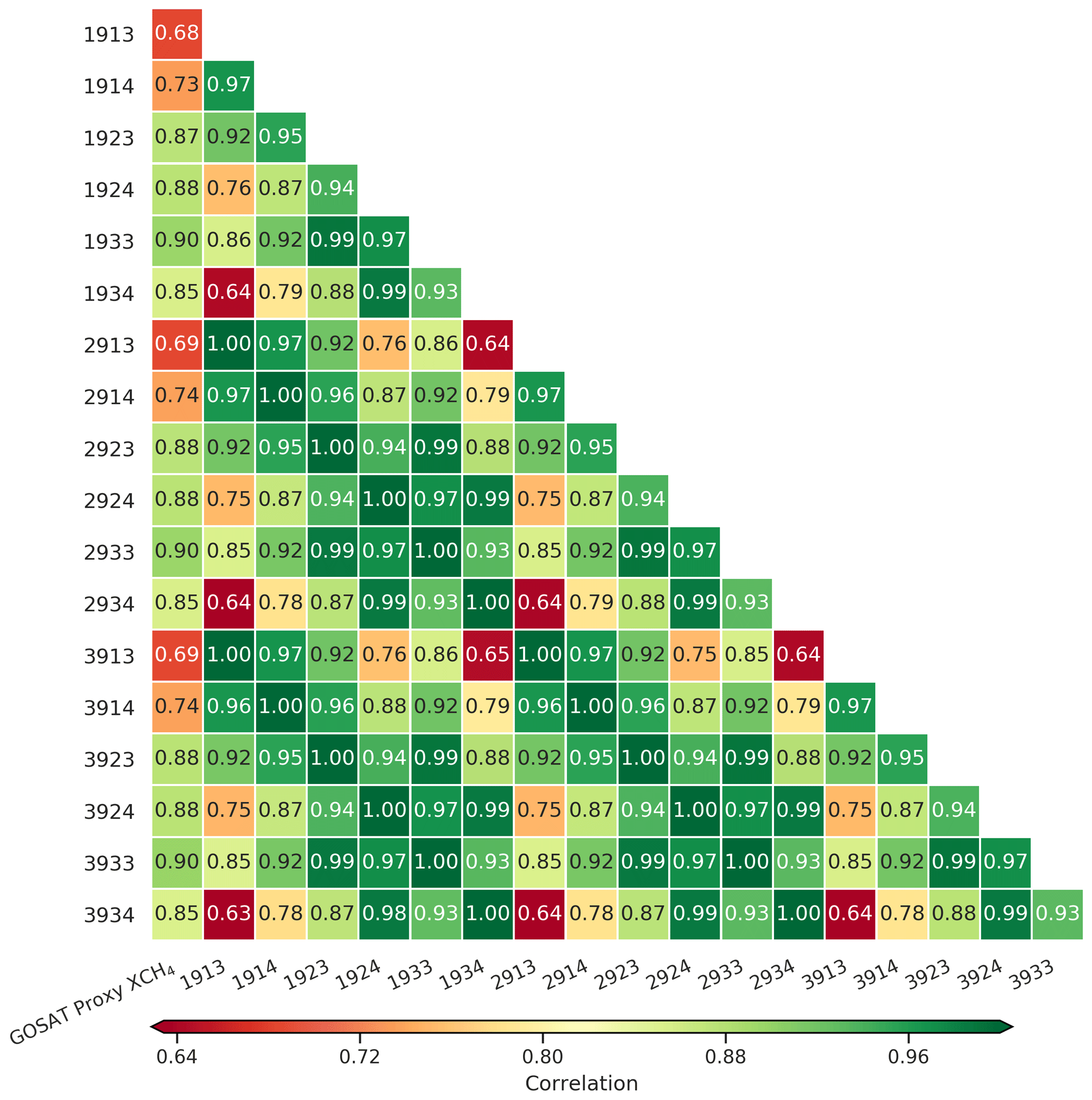
Figure 2Global correlation coefficient between the wetland CH4 seasonal cycle derived from the GOSAT Proxy XCH4 and each WetCHARTs ensemble member (leftmost column) and also between individual ensemble members.
This section evaluates the WetCHARTs ensemble by computing global statistics comparing the TOMCAT model simulations against the GOSAT XCH4 observations. In order to properly compare the model to observations, the model simulations are all sampled at the time and location of the GOSAT measurement and a total column model XCH4 value is computed with the GOSAT averaging kernel applied. Globally between 2009 and 2017 we have 3 382 474 GOSAT XCH4 observations, with 2 075 699 over land and 1 306 775 over ocean. In this study we restrict our analysis to the observations over land to focus on CH4 emissions.
To assess how representative the WetCHARTs emission ensemble is of the observed wetland CH4 seasonal cycle, we calculate the smoothed detrended seasonal cycle by applying the NOAA ccgcrv curve-fitting tool (Thoning et al., 1989) to the XCH4 data for the GOSAT observations and for each ensemble member. We also apply this routine to the TOMCAT model simulation that has no wetland CH4 emissions included. The seasonal cycle from this “no-wetland” simulation is subtracted from all other seasonal cycles, resulting in data representing only the wetland component of the seasonal cycle. This makes the assumption that wetlands dominate the uncertainty in interannual variability in the CH4 emissions and the remaining CH4 sources are in comparison far less uncertain. It should be noted that there is the potential for our assumptions regarding biomass burning emissions to interfere with our derived wetland seasonal cycle. However, we have carried out full global inversions of CH4 flux using this GOSAT data product and this chemical transport model (Wilson et al., 2020) which suggest that this is not a significant issue. Whilst it is difficult to separate out the fire emissions from other emission sectors using this methodology, our findings suggest that flux changes in burning regions in South America and Africa during the burning season generally change relatively little from the prior, compared to nearby wetland regions. However, it is true that in some extreme years (e.g. 2010 drought in S America), there are more significant changes to the GFED prior derived by the inversion. Although wetland and burning regions are often spatially distinct, this could affect some of our results to a small extent.
We first perform this analysis globally and in later sections separately for data within each region of interest. Figure 2 shows the correlation coefficients between the wetland CH4 seasonal cycles when calculated globally. The left column shows the correlation against the GOSAT-derived seasonal cycle, whilst the remaining columns show the model–model correlations for different pairs of ensemble members. It should be noted that the high correlation between certain groups of ensemble members is expected (e.g. for members 1913, 2913 and 3913 where the only configuration difference is the global scaling factor). The correlation against observations highlights that when considered at a global scale, the temperature dependence is clearly important. The ensemble members where there is no temperature dependence (i.e. Q10=1, ensemble members xx1x) all correlate far more poorly to observations than the same configuration including temperature dependency (e.g. r=0.69 for ensemble member 2913 vs. r=0.88 for ensemble member 2923). While it is clear that some temperature dependence is important, it is not clear from analysis at a global scale what degree of temperature dependence gives the best agreement with observations. Instead, regional analyses as performed in Sect. 6 are required.
The other feature of note in Fig. 2 is the variability in the inter-ensemble correlation coefficients. For example, correlations between pairs of WetCHARTs-based TOMCAT simulations can be as low as 0.63 (ensemble member 3934 vs. ensemble member 1913). In fact, the correlation coefficient is extremely poor (r = 0.63–0.65) for all simulation pairs where the temperature dependency is at the opposite extreme and the alternate wetland extent dataset is used. This further reinforces the need to continue this analysis at a regional scale to understand the driving factors for these differences over a range of wetland ecosystems.
Before performing a detailed regional evaluation, it is useful to consider how the varying WetCHARTs ensemble parameters are responsible for the variation in the subsequent WetCHARTs emissions. For this purpose we perform a variance analysis by calculating the partial correlation (Vallat, 2018) between time series for each parameter and the resulting WetCHARTs emissions. To clarify, this analysis is purely an assessment of the WetCHARTs CH4 emissions against its own driving data used to generate those emissions. It is not intended to be interpreted as a general statement about the importance of these parameters to explaining the variance in the real world. This assessment is useful because if a certain driver is dominating the response in WetCHARTs emissions and we subsequently observe discrepancies in the CH4 measurements, this indicates further evaluation of that driving data may be useful. It should be noted however that for the extended time period examined here we only have one heterotrophic-respiration model available and the contribution of heterotrophic-respiration uncertainty within the WetCHARTs full ensemble is considerable due to model disparities in mean emission rates and the corresponding seasonal cycles (see Fig. 6 in Bloom et al., 2017b). Ultimately further expansion and exploration of the heterotrophic-respiration model ensemble may prove useful for robustly representing the terrestrial C-cycling uncertainty.

Figure 3Explained variance (R2) calculated as the individual partial correlation between the seasonal cycle of the WetCHARTs CH4 emissions and the seasonal cycles in the wetland extent fraction, temperature dependency and heterotrophic respiration for each region that were used to derive the WetCHARTs emissions. These values are averaged across all ensemble members to give an indicative value for the sensitivity of each region to the different driving parameters. Note that due to potential cross-correlations, it is not necessarily expected that the percentages sum to 100 %.
We average the result across all ensemble members to derive an indication of which drivers (extent, temperature and respiration) are important in which regions (Fig. 3). We also use this figure as an opportunity to identify the geographic extent of the different wetland regions used throughout this study.
When considered globally, no one parameter is found to be the primary driver of the variation in the WetCHARTs emissions, with the R2 value ranging from 29 % to 37 %. For the Southern Hemisphere however, the wetland extent fraction itself is found to explain 83 % of the variation in the emissions, with the temperature dependency and respiration both explaining approximately a third on their own.
When performing this analysis in smaller regions, individual behaviours become more apparent. For example, variations in heterotrophic respiration are found to be much more important in some regions such as the West Amazon where they can explain 45 % of the variations in the WetCHARTs emissions, whereas for the Sudd region they only explain 6 % of the variation in the emissions. Likewise, the temperature dependency explains 63 % of the variance in China and over 40 % in many regions (West Amazon, Pantanal, Paraná, Sudd and Southern Africa) but only a few percent in other regions (Yucatán, East Amazon, Indonesia, Papua, SE Australia).
The wetland extent is found to be the dominant explanation for the variance in all regions, often by a large margin, explaining >95 % of the variance in the Yucatán, West Amazon, East Amazon, Pantanal, Congo, Indo-Gangetic, SE Asia and N Australia regions. Even for the regions where the wetland extent explains the least variance such as East USA (72 %), Sudd (64 %), China (79 %) and SE Australia (75 %), it still explains more than the other parameters.
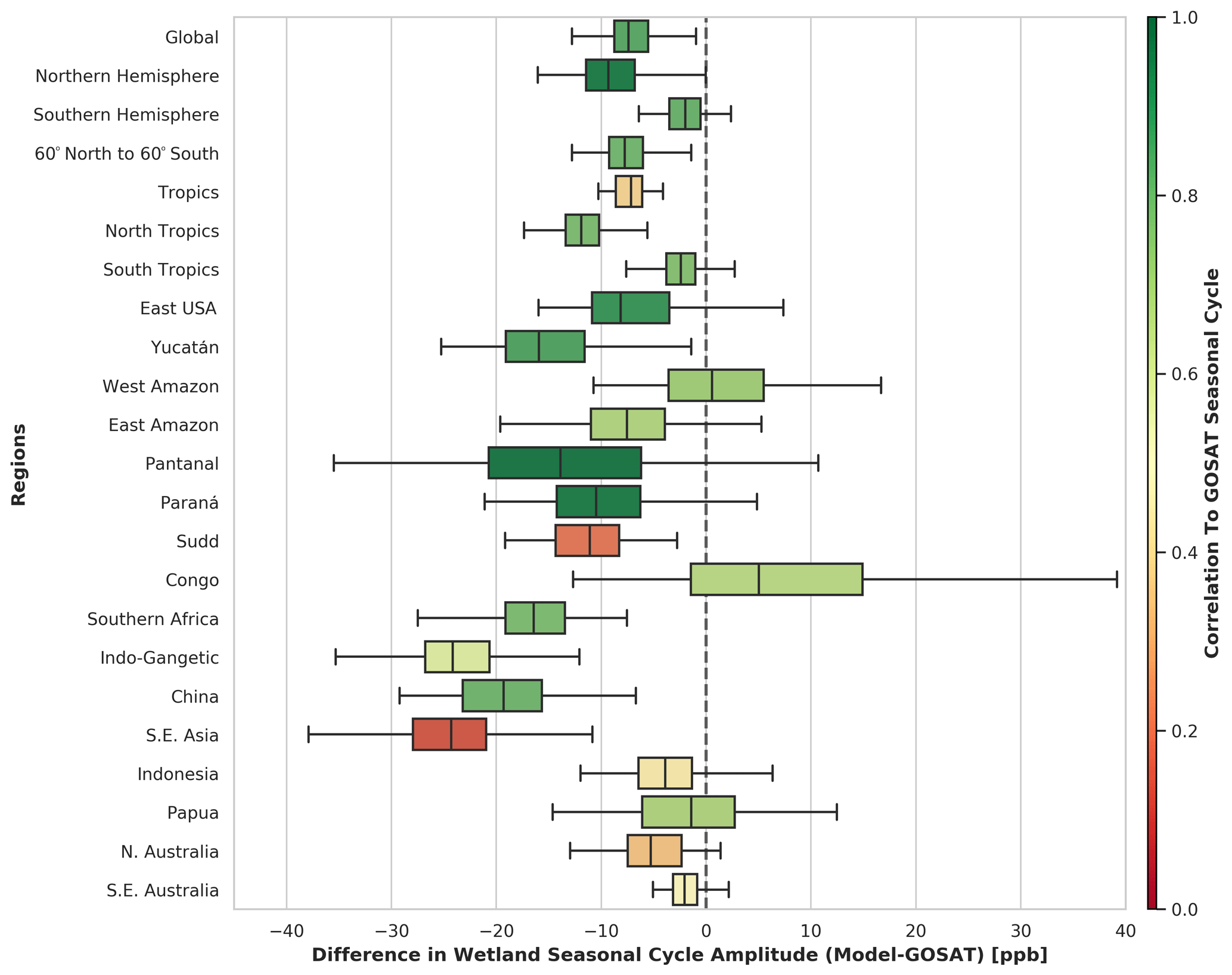
Figure 4Distributions of the wetland CH4 seasonal-cycle amplitude difference between the modelled WetCHARTs and GOSAT observations for all ensemble members and all years for the different regions. The data are coloured by the average value of the correlation coefficient between the modelled and observed wetland CH4 seasonal cycle. The median and 25th and 75th percentiles are indicated by the boxes, with the full range indicated by the whiskers.
The capability of the WetCHARTs emissions to successfully represent the observed wetland CH4 seasonal-cycle amplitude is a vital component in the assessment of the utility of the emissions. In addition to assessing the seasonal amplitude we assess the magnitude and phase of the emissions using the correlation coefficient between the simulated and observed seasonal cycles. Figure 4 shows the distributions of the wetland CH4 seasonal-cycle amplitude difference between the model and observations for all ensemble members and all years for the different regions. Furthermore, each bar is coloured by the ensemble-average correlation coefficient between the wetland CH4 seasonal cycle of the WetCHARTs ensemble members and the GOSAT observations.
There is a clear hemispheric distinction between the difference in seasonal-cycle amplitude, with the underestimation being far more pronounced in the Northern Hemisphere (9.3 ppb) than in the Southern Hemisphere (1.9 ppb). This is further emphasised by considering the tropical region only; the North Tropics (0∘ to 30∘ N) underestimates the seasonal-cycle amplitude by 11.9 ppb, compared to just 2.4 ppb in the South Tropics (0∘ to 30∘ S).
When considering comparisons on a regional scale, it is possible to characterise the different regions into groups that exhibit similar behaviour.
For some regions the seasonal-cycle amplitude is always significantly underestimated for all years and for all ensemble members. This is particularly the case for Southern Africa, China, SE Asia and the Indo-Gangetic region, where WetCHARTs underestimates the observed seasonal cycle by median values of −16.6, −19.1, −23.1 and −24.2 ppb respectively.
This, however, is not the case for all regions, with some regions such as West Amazon, Papua, Indonesia and the Congo exhibiting a small median difference in the seasonal cycle (+0.7, −1.2, −4.0 and +5.0 ppb respectively) but with a large variability between years and ensemble members. The Congo region in particular exhibits a large variability in the seasonal-cycle amplitude difference (−12.7 to 52.4 ppb) despite the reasonable correlation to the observed seasonal cycle (r=0.67).
Some regions (East USA, Pantanal, Paraná, Yucatán) have a high correlation to the observed seasonal cycle (0.88, 0.94, 0.93 and 0.84) but consistently underestimate the amplitude (−7.7, −14.1, −10.5 and −15.8 ppb) and also contain a large amount of variability between the different ensemble members and years.
Finally, the underestimation of the seasonal-cycle amplitude can be similar to those described above (−11.2 ppb) but with a very poor correlation to observations (r=0.20), as observed for the Sudd region.
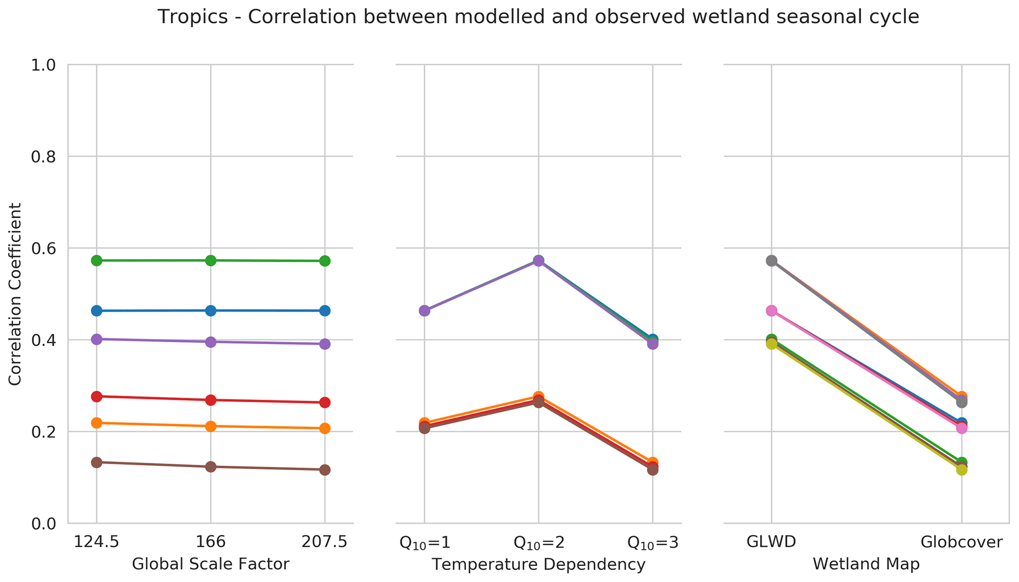
Figure 5For each of the three parameters that vary within the ensemble (global scale factor, temperature dependency and wetland extent map), we plot the correlation coefficient between the modelled and observed wetland CH4 seasonal cycle. We join data points where the other two parameters are kept constant, and the only change is due to the specified parameter. The line colours are to indicate the different combinations within each panel. Due to the nature of the plot, there is no link between colours in different panels as they represent different pairs or trios of data. For example, for temperature dependency, we join the three data points where the temperature dependency varies between Q10=1, Q10=2 and Q10=3 but the wetland map and the global scale factor are the same for the three joined data points. This allows the influence of the change in each individual parameter to be assessed.
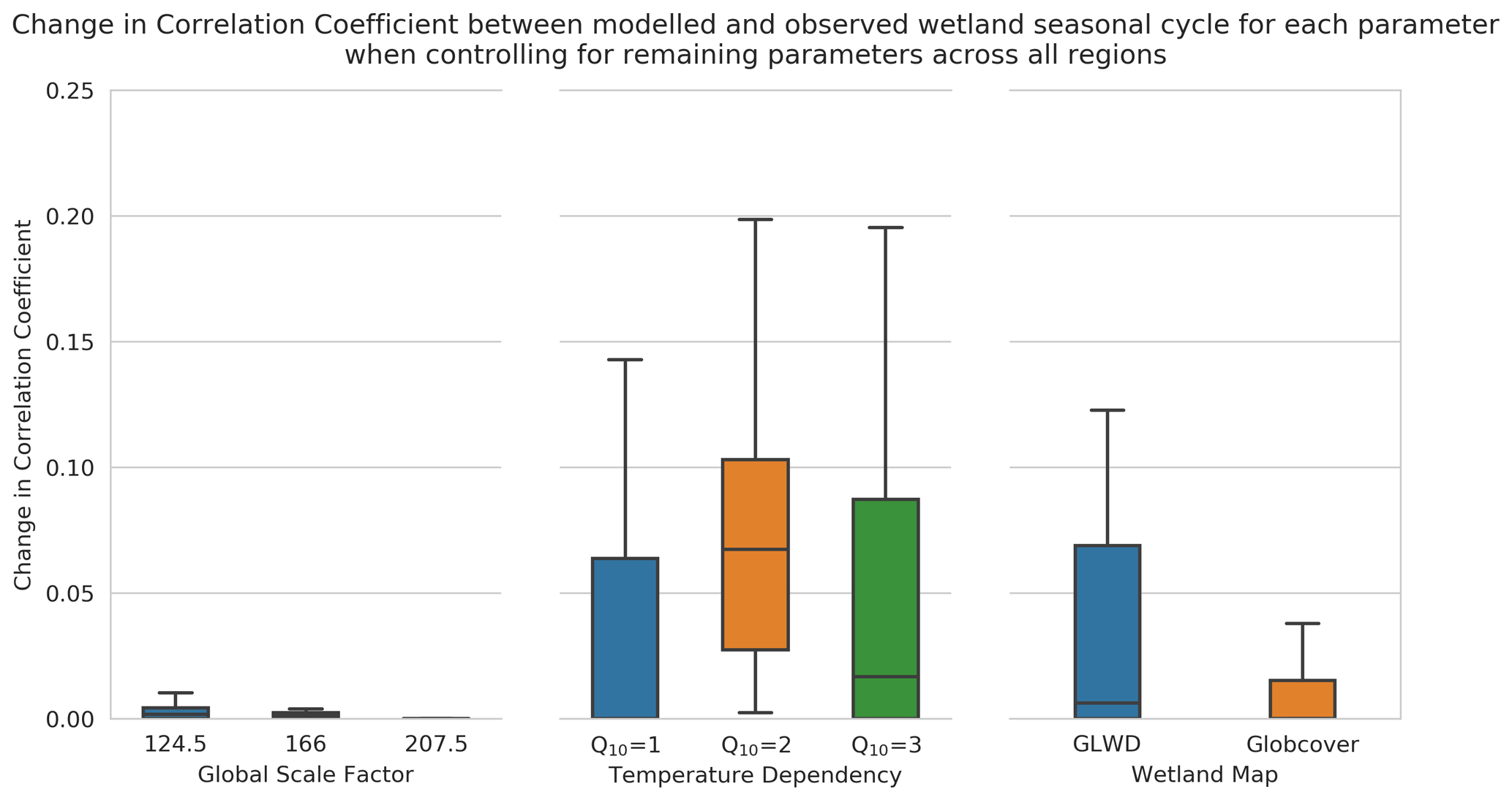
Figure 6The change in correlation coefficient between the modelled and observed wetland CH4 seasonal cycle related to each parameter with all other parameters kept constant. The change is calculated as the improvement in correlation coefficient from the lowest value from each set of joined ensemble members. The distribution of this change in correlation coefficient across all regions is illustrated using a box-and-whisker plot with the quartiles indicated by the boxed area and whiskers indicating the remaining data (excluding extreme outliers).
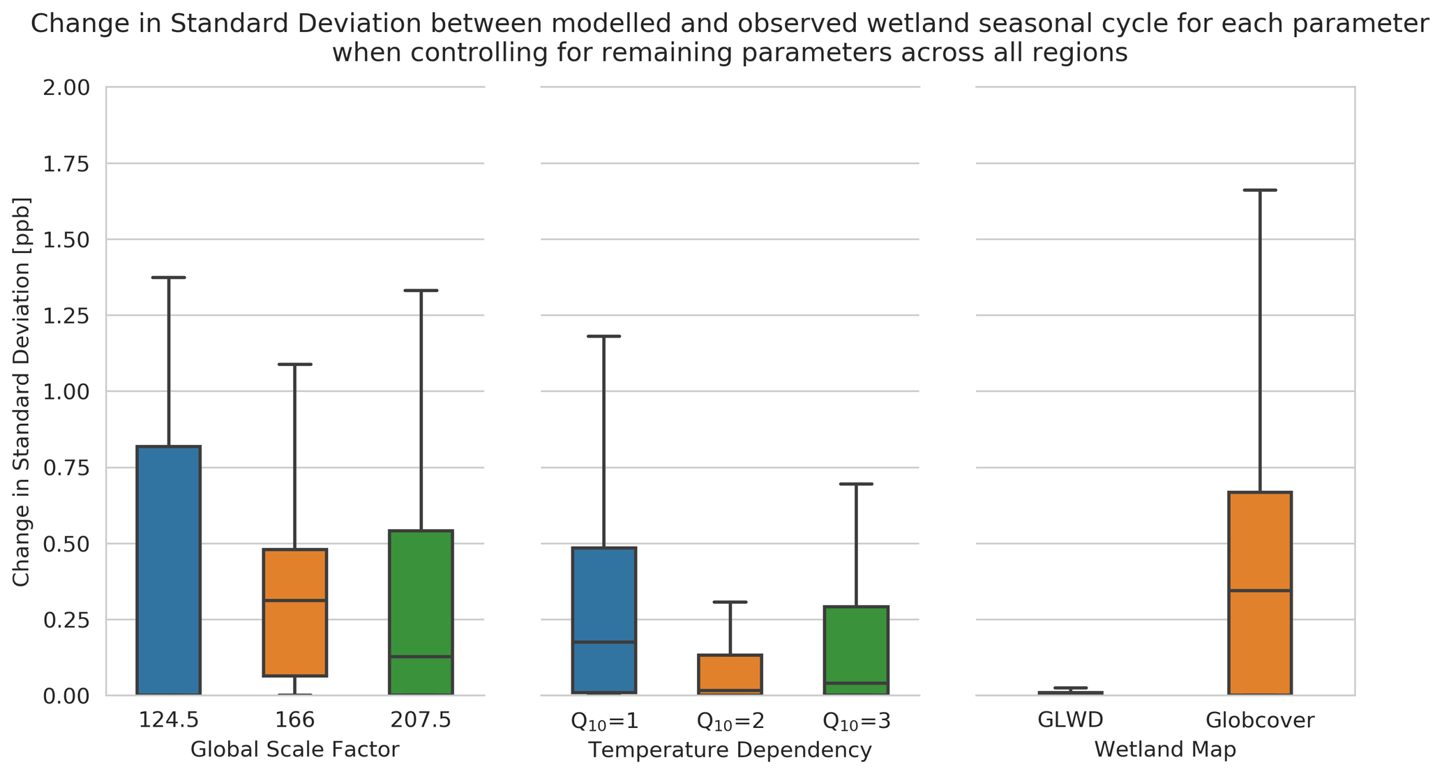
Figure 7The change in standard deviation (ppb) between the modelled and observed wetland CH4 seasonal cycle related to each parameter with all other parameters kept constant. The change is calculated as the difference in standard deviation from the lowest value from each set of joined ensemble members. The distribution of this change in standard deviation across all regions is illustrated using a box-and-whisker plot with the quartiles indicated by the boxed area and whiskers indicating the remaining data (excluding extreme outliers).
In order to understand the effect that the different WetCHARTs parametrisations have on the different regional emissions, the correlation coefficient and standard deviation between the simulated and observed seasonal cycle are calculated for each region for each ensemble member. The full table of correlation coefficients per region per ensemble member is presented in Appendix A (Fig. A1). To highlight and isolate the individual effects of adjusting the three driving parameters (global scale factor, temperature dependency and wetland extent map), we plot the correlation coefficient for each configuration of the ensemble and link together data points where the only change between the ensemble members is the change in the specified parameter. This is demonstrated for the Tropics (30∘ S to 30∘ N) in Fig. 5. In this figure we see that the correlation coefficient is largely unaffected by a change in the global scale factor, when controlling for the other parameters. In contrast, a temperature dependency of Q10 = 2 clearly leads to a higher correlation coefficient for the Tropics, when controlling for the other parameters, with Q10=3 leading to the worst correlation coefficient in all cases. Similarly, it is evident that the GLWD wetland extent map performs significantly better than the GlobCover map, significantly increasing the correlation coefficient in all cases.
To emphasise the effect related to the relative change of each parameter when considering the behaviour across multiple regions, we subtract as a baseline the lowest correlation coefficient from each set of lines. This change in correlation coefficient therefore gives an indicator of the improvement obtained by the change in each parameter while keeping the rest of the configuration for that ensemble member the same. Figure 6 shows the distribution of this change in the correlation coefficient across all regions. These results illustrate that the choice of the global scale factor makes little difference to the correlation between the observed and modelled wetland CH4 seasonal cycle. In contrast, the choice of the Q10 value is found to make a substantial difference to the correlation coefficient. Setting Q10=1 typically produces the worst correlation coefficient (as indicated by a median value of 0 improvement), with Q10=2 typically leading to the largest improvement in the correlation coefficient (with a median value of 0.067 and an improvement of up to 0.20). On average, Q10=3 does not perform as well in a general sense (a median value of 0.017), but it does produce a large spread in values, indicating that for some regions it does lead to better performance. Finally for the wetland extent, it is very clear that the GLWD wetland extent map performs better for the majority of regions, leading to an improvement (75th percentile) of 0.069 in the correlation coefficient compared to just 0.015 for GlobCover.
As well as the correlation between the modelled and observed seasonal cycle, the standard deviation between the two is a useful metric for determining how well the WetCHARTs emissions allow the seasonal cycle to be reproduced. In Fig. 7 we examine the increase in standard deviation related to each parameter, with a smaller value indicating better performance. In contrast to the analysis of the correlation, we find that the choice of global scale factor does have an impact here. The global scale factor of 124.5 Tg yr−1 has the lowest median change in standard deviation (0.0 ppb, indicating it is always the lowest and best on average) but exhibits a large spread across regions (75th percentile of 0.82 ppb). The medium global scale factor of 166 Tg yr−1 is much more consistent across regions with a smaller spread (75th–25th range of 0.42 ppb vs. 0.82 ppb) but on average produces a larger standard deviation than the lower scale factor (median value of 0.31 ppb). For temperature dependency, the picture is clearer, with Q10=2 producing the smallest median standard deviation (0.016 ppb) and the smallest spread (75th–25th range of 0.13 ppb). Finally, the GLWD wetland map is found to perform emphatically better than the GlobCover map for nearly every region, with GlobCover on average worsening the standard deviation by an average 0.34 ppb and up to over 4 ppb in some cases.
When considering the two metrics (correlation coefficient and standard deviation) in unison, a consistent conclusion can be drawn that a temperature dependency can cause large changes in the agreement between the model and the observations, with a Q10=2 value typically performing better on average but Q10=3 performing better for some regions. Both results suggest that some temperature dependency is necessary, i.e. that Q10=1 performs worse than the alternatives. Likewise, the GLWD wetland extent map is consistently found to perform better than the GlobCover map. Whilst the global scale factor is found to have little influence on the correlation coefficient, it does influence the standard deviation between the modelled and observed wetland CH4 seasonal cycle.
This summary of the regional analysis points towards complex interactions and highlights the difficulty in using a simple parametrisation to represent many complex inter-related processes. A more detailed analysis of exemplar regions as case studies is valuable in explaining the above-described behaviours in more detail.

Figure 8Modelled – GOSAT monthly mean wetland CH4 seasonal-cycle differences for all WetCHARTs ensemble members from 2009 to 2017 over the Paraná region.
Figure 9MODIS Normalized Difference Water Index (NDWI) indicating surface water extent for November–April from 2010 to 2017 overlaid onto MODIS RGB imagery for the Paraná region.
In Parker et al. (2018) we identified the Paraná River as a particularly interesting example of a case where excess precipitation led to severe overbank inundation, which was clearly evident in multiple ancillary datasets (MODIS visible imagery, GRACE Terrestrial Water Storage Anomaly, etc). This large but temporary increase in wetland extent produced significant methane emissions which were clearly observed from satellite observations but which were missing from any model simulations as this inundation mechanism was not represented in the underlying emission datasets.
Our previous analysis identified a large anomalous event in 2010, but the analysis ended in 2015. For this work we are able to extend this analysis until the end of 2017. The monthly mean difference between the simulated and observed wetland CH4 seasonal cycles over this region are shown in Fig. 8. The large 2010 anomaly, where simulations are all significantly less than the observations, is again observed, but in addition, we observe similarly large anomalies in 2016 and 2017. These large anomalies are persistent across all model ensembles but are at a minimum for the more intense emission scenarios (large scale factor and larger temperature dependency) and when the GLWD wetland extent parametrisation is used.
A comparison to the MODIS Normalized Difference Water Index (NDWI; Fig. 9) explains the nature of the anomalies observed above. For 2010, 2016 and 2017 there were significant increases in river inundation along the channel of the Paraná River, especially in the Paraná Delta region to the north of Buenos Aires. The resulting CH4 emissions from this increase in wetland extent are clearly observed by GOSAT but are not represented within the WetCHARTs model ensemble, leading to the model ensemble monthly mean under-representing the observed CH4 amount by up to −8.5, −8.2 and −9.4 ppb for 2010, 2016 and 2017 respectively. For the remaining years of the analysis (2011–2015) which correspond to the years when the NDWI extent is noticeably lower, the agreement between the WetCHARTs ensemble and the observation data is far better with maximum differences of −3.5, −4.7, −5.8, 3.0 and −7.5 ppb respectively. Furthermore the annual range of standard deviations of the ensemble monthly mean differences for 2010, 2016 and 2017 is considerably higher (3.9–5.4 ppb) than for the 2011–2015 period (2.3–3.7 ppb). This again highlights the increased variability during 2010, 2016 and 2017 and the characterisation of these years as anomalous, driven by the significant change in observed wetland extent related to the inundation of the Paraná River and Paraná Delta.
This case highlights one limitation of WetCHARTs, namely that there is no underlying hydrological model to account for river flow or inundation but instead local precipitation determines the wetland extent variability. As such, WetCHARTs may not capture the behaviour where wetland extent is determined by behaviour upstream. This, however, allows WetCHARTs to act as a baseline against which to assess such behaviour in land surface models and determine if they are outperforming the simpler WetCHARTs precipitation-driven approach.
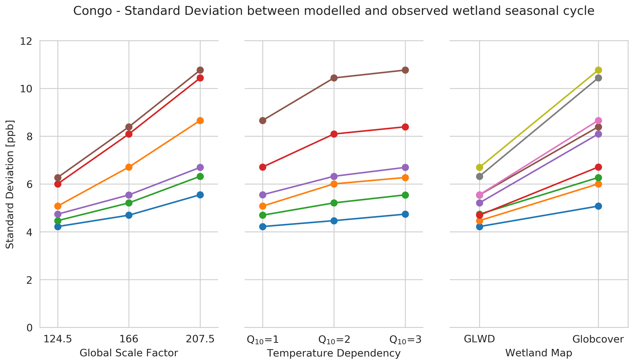
Figure 10The standard deviation between the modelled and observed wetland CH4 seasonal cycle for each of the three parameters that vary within the ensemble (global scale factor, temperature dependency and wetland map). Data points are joined together where the other two parameters are kept constant, and the only change is due to the specified parameter. This allows the influence of the change in each individual parameter to be assessed.
The Congo is perhaps one of the most important wetland regions to be able to well characterise as it has the potential to dominate African methane wetland emissions but is still relatively poorly understood (Lee et al., 2011; Melton et al., 2013; B. Zhang et al., 2017; Becker et al., 2018; Lunt et al., 2019).
Figure 4 highlights the huge discrepancy between the observed wetland CH4 seasonal-cycle amplitude from GOSAT and that simulated by any of the WetCHARTs ensemble members (a median difference of 5 ppb but ranging from −12.7 to 52.4 ppb). This is consistent with recent work in both Lunt et al. (2019) and Maasakkers et al. (2019) which uses WetCHARTs data as the prior in atmospheric flux inversions. In Lunt et al. (2019), flux inversions of atmospheric CH4 over Africa suggest that the mean WetCHARTs emissions over the Congo region are far too high (8.5 Tg yr−1 in total with 90 % of this attributed to wetlands) and need to be reduced significantly to be consistent with observations in the range of 2.7–4.1 Tg yr−1. This is also more consistent with Tathy et al. (1992), who estimate methane emissions within the flooded Congo Basin using flux chamber measurements of 1.6–3.2 Tg yr−1. Maasakkers et al. (2019, Fig. 4 therein) show similarly that the posterior emissions after inversion of the GOSAT data require a reduction to the original WetCHARTs prior emissions over the Congo region.
Figure 10 demonstrates that the standard deviation of the model–GOSAT difference is substantially worsened when either the temperature dependency (xxCx ensemble members, increasing from a median of 5.31 to 6.48 ppb) or the global scale factor (Axxx ensemble members, increasing from a median of 4.91 to 7.68 ppb) is increased. This is indicative of there already being too much CH4 from WetCHARTs in this region, and any parametrisation that enhances it further (by either scaling or adding a temperature dependency) exacerbates the discrepancy. This points to the wetland extent fraction being too large, and this wetland extent masking clearly plays a significant role as the standard deviation differs substantially based on which extent mask is being used, ranging from 4.22 to 6.70 ppb for the GLWD-based ensemble members but 5.08–10.77 ppb for the GlobCover-based simulations. The different wetland extent masks however do not affect the correlation coefficient between the simulated and observed seasonal cycles (Fig. A1), suggesting that both wetland masks are equally capable of parameterising the observed seasonal cycle but differ in the magnitude of the resulting emissions. Figure 12 compares both wetland extent datasets against the JRC surface water occurrence and maximum extent datasets (Pekel et al., 2016), confirming that the wetland extent used in WetCHARTs is significantly higher than suggested by the JRC data.
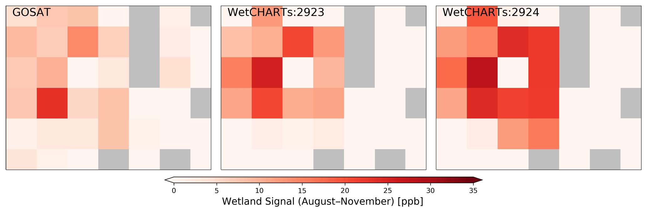
Figure 11The average wetland signal for August–November between 2009 and 2017 over the Congo region. The wetland signal is defined as the difference between the detrended GOSAT or WetCHARTs model simulations and the simulation with no wetland emissions. Two WetCHARTs ensemble members are shown (2923 and 2924) for illustration, but all ensemble members exhibit similar behaviour.
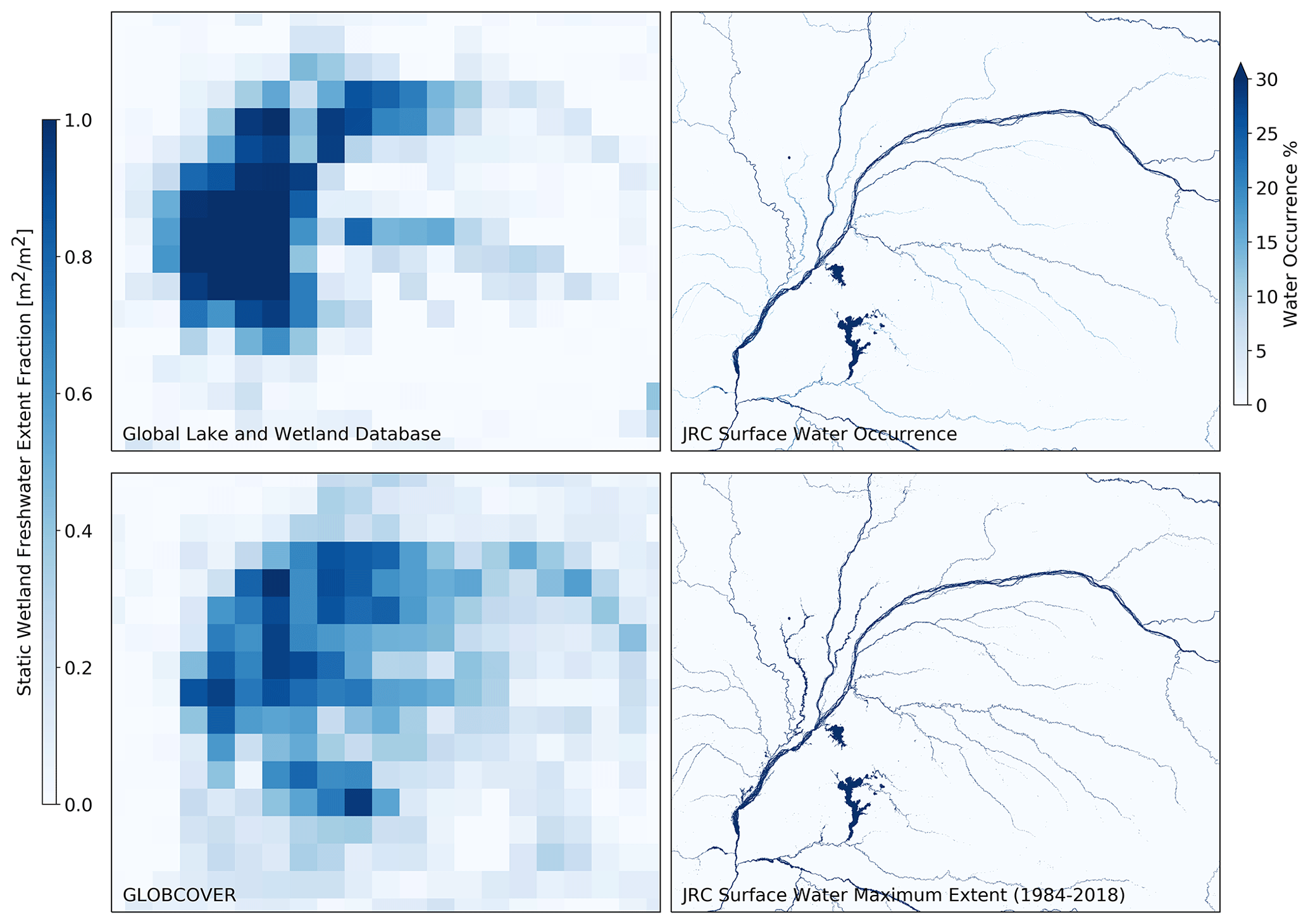
Figure 12Maps over the Congo region showing the GLWD and GlobCover wetland data used to drive WetCHARTs compared to the JRC surface water occurrence and maximum extent datasets.
Although the spatial resolution of GOSAT is relatively coarse (∼ 250 km), Fig. 11 shows that it is possible to identify the spatial signature of the wetland signal in both the GOSAT observations and the model simulations (sampled at the GOSAT sounding locations). The GOSAT wetland signal (i.e. the difference to the simulation without any wetland emissions) is relatively weak, with a maximum (95th percentile) value of 11.9 ppb. We compare this to WetCHARTs ensemble members 2923 and 2924 (chosen to be illustrative of the wider ensemble with the medium global scaling factor and medium temperature dependency). The maximum wetland signal from the WetCHARTs 2923 and 2924 ensemble members is much stronger than that derived from GOSAT, with values of 20.5 and 23.6 ppb respectively. As well as a much smaller maximum signal, the spatial standard deviation of the wetland signal for GOSAT is found to be 6.8 ppb, much smaller than the standard deviations from WetCHARTs of 11.3 ppb (2923) and 15.1 ppb (2924).
This demonstrates that while the spatial signature of the Congo wetland emissions generated by WetCHARTs is reasonably consistent with that from observations, the magnitude of and variability in the emissions are far higher than those we observe from GOSAT. This remains the case for the smallest global scale factor and for no temperature dependency, leaving only the wetland fraction or heterotrophic carbon respiration per unit area as tuning parameters to reduce the emissions to be closer to observations. Various published atmospheric inversions of our CH4 data that have used WetCHARTs as the prior all indicate that the Congo emissions are overestimated by WetCHARTs and reduced when confronted with observations. This highlights the large uncertainty over this region. Once the necessary MsTMIP (or similar) model data become available and it is possible to extend the WetCHARTs full ensemble (i.e. all respiration models) to this time period, we will revisit this question in a future study.
This case highlights that future WetCHARTs development would benefit from further exploration of the characterisation of and sensitivity to the heterotrophic respiration, with the extended ensemble currently only featuring a single member (CARDAMOM).
In this section we examine the Sudd wetland region. The Sudd wetlands, located in South Sudan, are one of the largest tropical wetlands in the world and are the largest wetland ecosystem in the Nile Basin. They are fed via the White Nile, originating at Lake Victoria to the south with flow through the region ultimately leading into the Nile to the north. These wetlands therefore play a major role in regional hydrology, and understanding their behaviour is of vital importance for environmental, economic and humanitarian reasons.
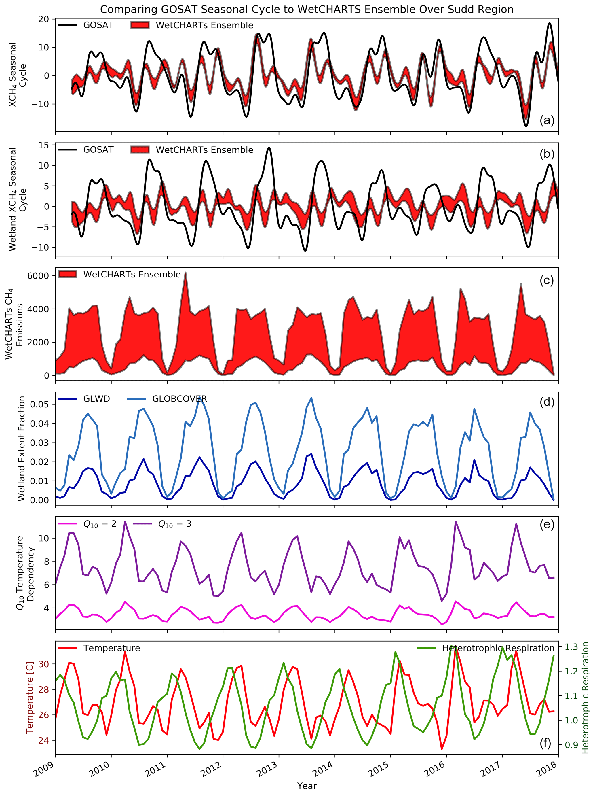
Figure 13Time series over the Sudd wetland region showing (a) the GOSAT and WetCHARTs CH4 ensemble seasonal cycle, (b) the wetland component of the above seasonal cycles once the modelled data with no wetland emissions have been subtracted, (c) the ensemble of WetCHARTs CH4 emissions, (d) the wetland extent fractions, (e) the Q10 temperature dependencies, and (f) the temperature and heterotrophic respiration.
The extent of these wetlands is driven by seasonal inundation and outflow from Lake Victoria (Rebelo et al., 2012), albeit significantly affected by the complexities of the regional hydrology. The wetland extent exhibits a maximum each year between August and November, coincident with the rainy season. This seasonal flooding has been estimated by Rebelo et al. (2012) to increase the wetland extent in the region by a factor of 4, with the total wetland area split between permanent (18 %) and seasonally inundated (82 %) wetlands. MODIS NDWI data (not shown) indicate that as well as the increase in surface water directly over the Sudd wetland region, there is also increased surface water evident further to the north of the region around Lake Tana and the Blue Nile Basin.
The results for this region are of particular interest as whilst the discrepancy between the magnitude of the simulated and observed seasonal cycles is comparable to other regions (−11.2 ppb), the correlation coefficient is extremely poor at just 0.2. This suggests that unlike many of the other regions where it is the magnitude of the seasonal cycle that WetCHARTs does not fully represent, this is one of the few regions where the seasonality is also poorly represented. This is illustrated by Fig. 13 which shows the GOSAT CH4 seasonal cycle over the Sudd region (black) along with the range of the WetCHARTs ensemble (red) for the full CH4 seasonal cycle (panel a) and with the no-wetland simulation subtracted, resulting in a wetland CH4 seasonal cycle (panel b). This wetland CH4 seasonal cycle shows that while observations have a clear seasonal cycle, with the signal ranging from −10.8 to 14.3 ppb, the typical seasonal cycle for the WetCHARTs ensemble is less than half of this (ranging between −6.7 to 6.3 ppb) and importantly does not seem to have any temporal agreement with the observations, resulting in the very poor correlation coefficients we obtain for all ensemble members.
The reason for this lack of sufficient seasonality in the WetCHARTs ensemble is evident when examining the time series of underlying driving data for the emissions (Fig. 13d–f). The seasonalities of both the temperature and the heterotrophic respiration are out of phase with the wetland extent. This results in there being either sufficient temperature and respiration to produce methane but no wetland area from which to produce it or, alternatively, a large wetland area but insufficient temperature and respiration to produce the correct magnitude of emissions. The effect of this is very limited seasonality in the CH4 emissions throughout the entire time series. This is exemplified in Fig. 14 which shows the average wetland signal for August–November (the time period where the satellite CH4 wetland signal peaks) between 2009 and 2017 for the GOSAT data (panel a) and two WetCHARTs ensemble members, 2923 (panel b) and 2924 (panel c). Despite the very strong wetland signal observed over this area, directly over the Sudd wetlands the WetCHARTs signal is extremely low. From Fig. 13, the seasonality of the two wetland extent parametrisations is in agreement with the seasonality of the observed signal, identifying that the issue in this area is not the dynamics of the wetland itself but rather the seasonality of the temperature and respiration which result in the magnitude of the emissions being far too small even though both wetland extent fraction databases allow WetCHARTs to form wetlands in this area. One limitation of skin temperature is the assumption that heterotrophic respiration is sensitive to top-of-soil temperature. We advocate for an expansion of the WetCHARTs ensemble to include subsurface soil temperature estimates – in place of surface skin temperatures – to explicitly represent the representation uncertainty associated with the soil temperature dependency of methanogenesis.
This case highlights an example where although the wetland extent is sufficient to lead to the correct seasonality in CH4 emissions, the temperature and respiration are out of phase, and as such, WetCHARTs can not reproduce the observed variability. This emphasises the importance of the interplay between the different driving parameters and the large discrepancy that can be caused if these are not consistent or sufficiently localised.
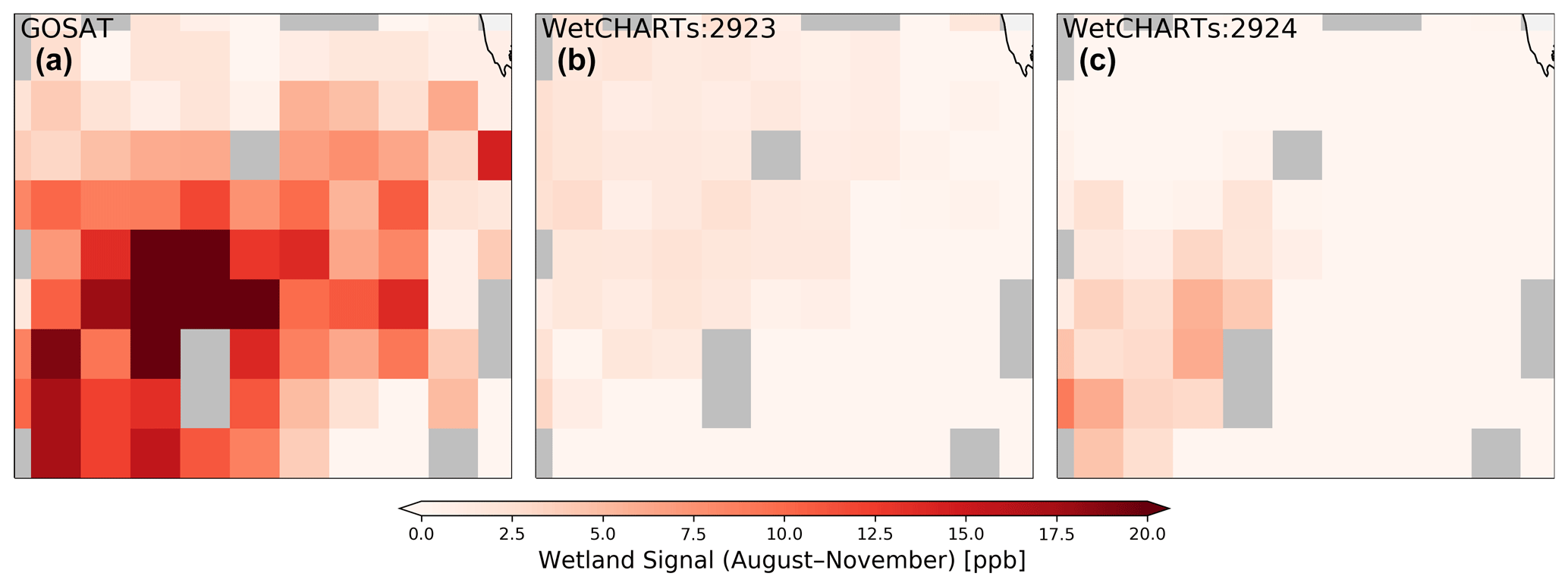
Figure 14The average wetland signal for August–November between 2009 and 2017 over the Sudd region. The wetland signal is defined as the difference between the detrended GOSAT or WetCHARTs model simulations and the simulation with no wetland emissions. Two WetCHARTs ensemble members are shown (2923 and 2924) for illustration, but all ensemble members exhibit similar behaviour.
The Yucatán area of Mexico contains a variety of wetland ecosystems including mangroves, swamps, marshes and forests with the watershed containing the Grijalva and Usumacinta rivers in the Tabasco–Campeche region, the largest wetland complex in the country. The Pantanos de Centla region, located in the Usumacinta–Grijalva delta, is classified as tropical moist forest and includes permanent wetlands as well as seasonally inundated swamp forests. Mangroves are present between the Pantanos de Centla and the Laguna de Términos to the north, with moist tropical forests to the south, east and west.
For the Yucatán region, the correlation between the observed and simulated wetland CH4 seasonal cycles is reasonable, with WetCHARTs ensemble members ranging from 0.76 to 0.89 (Fig. A1) suggesting that WetCHARTs is capable of representing the phase of the wetland CH4 seasonal cycle. However, Fig. 4 shows that the wetland CH4 seasonal-cycle amplitude is consistently underestimated compared to observations, with a median difference of −15.8 ppb and 25th- and 75th-percentile values of −19.1 and −11.5 ppb respectively. This underestimation of the seasonal cycle can be attributed to the very low wetland extent fraction from both the GLWD and GlobCover datasets (Fig. 15) which fails to represent the wetlands in this region, particularly the large Tabasco–Campeche wetland complexes in the centre of this region, the Alvarado Lagoon system to the west and the Sian Ka'an coastal wetlands to the east. These are barely included in either wetland extent dataset but are clearly identified as being significant from the JRC surface water extent (Fig. 15).
This case is of particular interest as it is one of the few examples where the Global Lakes and Wetlands Database performs particularly poorly, not featuring significant wetland extent that relates to a strongly observed wetland signal. The large difference between the wetland extent fraction from GLWD vs. GlobCover is also striking (Fig. 16) for this region, more so than in the other regions examined. Furthermore, both wetland extent datasets suggest a double peak in the maximum extent, leading to two peaks in the emission data. GOSAT observations however only typically observe the second of these peaks in most years.
This case highlights the importance of the wetland extent data and that while for the majority of regions it is the detail of the variability in extent that we are concerned with, for some regions the extent is even more poorly constrained with large wetland regions still not being represented.
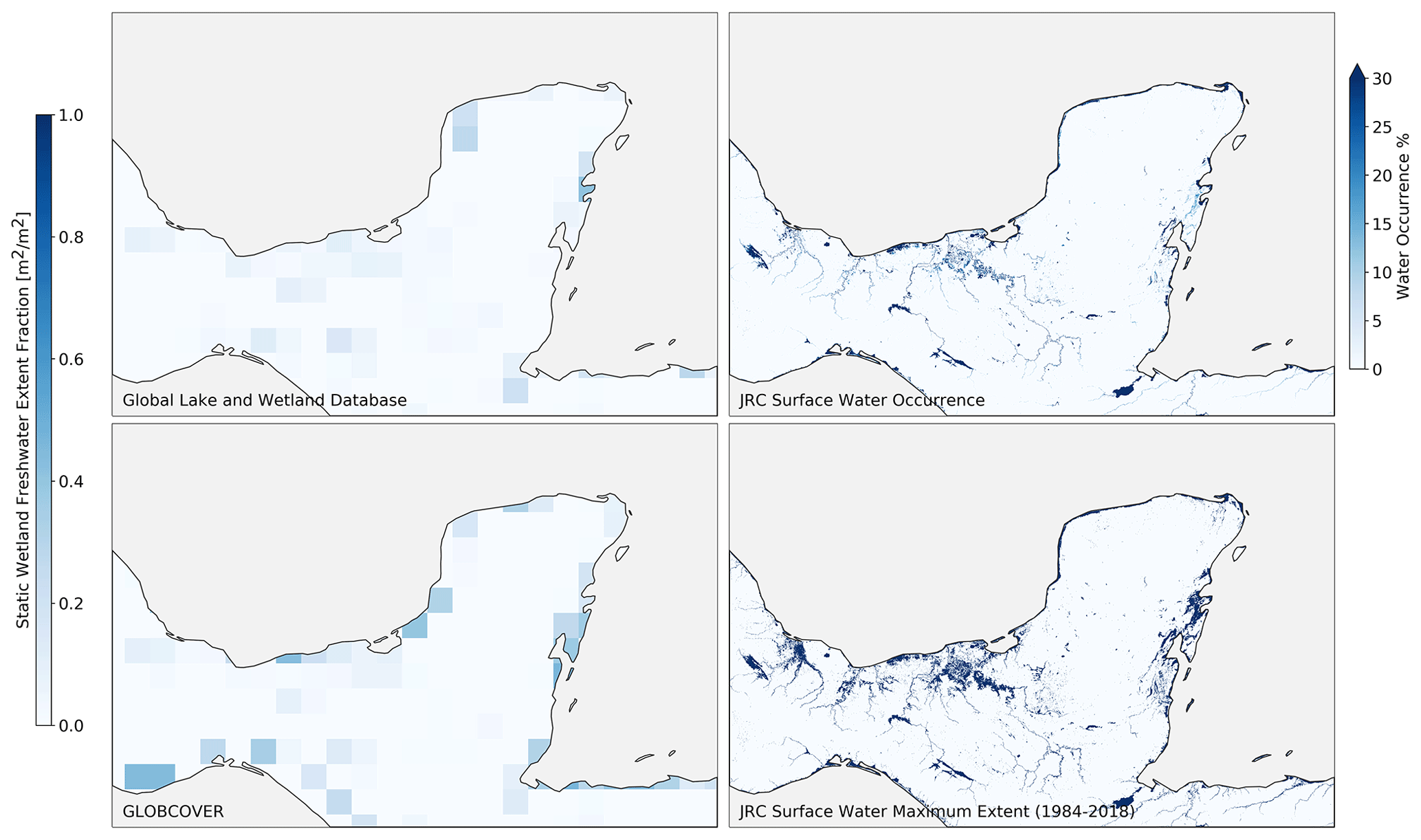
Figure 15Maps over the Yucatán region showing the GLWD and GlobCover wetland data used to drive WetCHARTs compared to the JRC surface water occurrence and maximum extent datasets. Neither of the datasets driving WetCHARTs represents the large Tabasco–Campeche wetland complexes in the centre of this region.
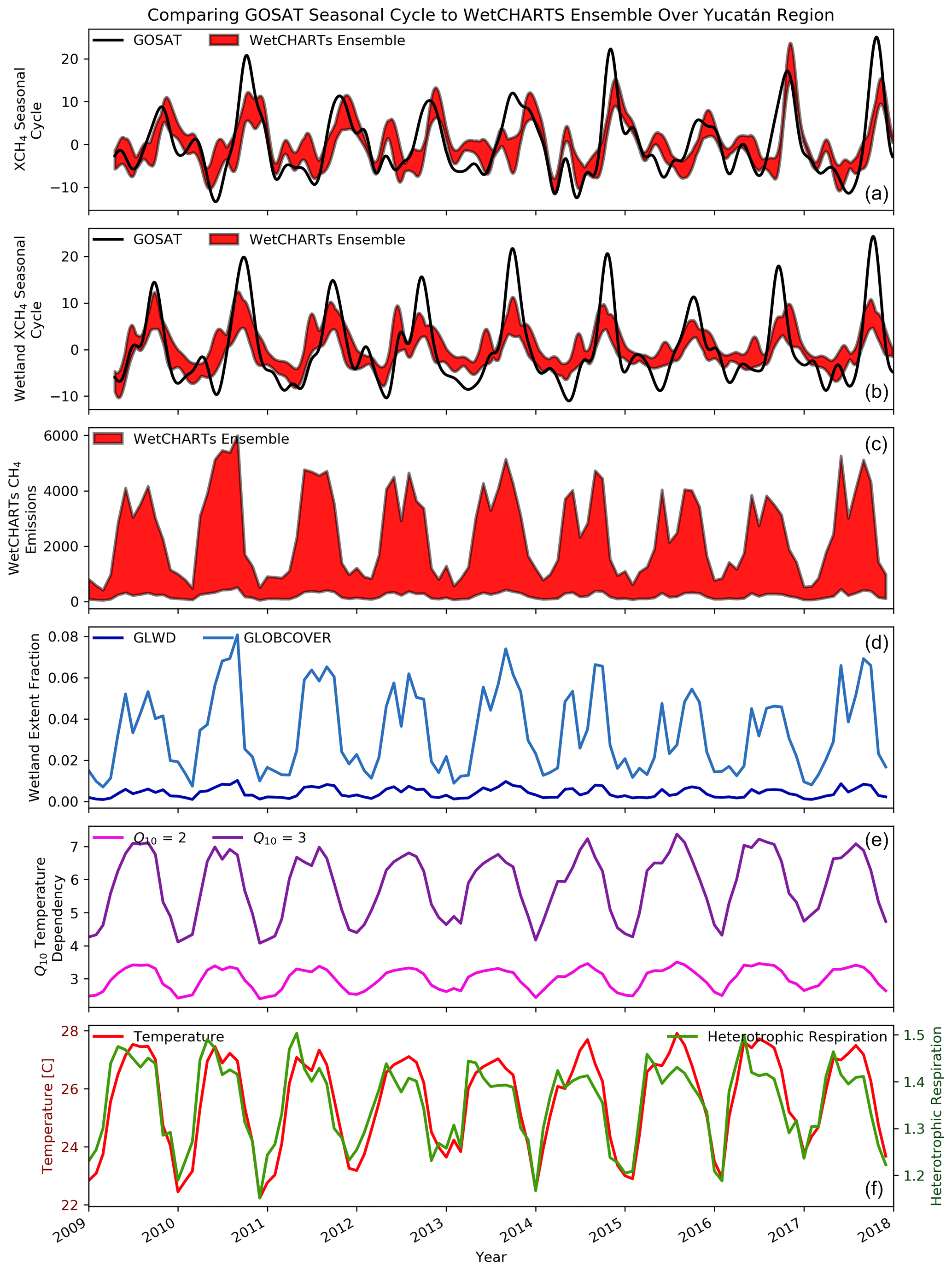
Figure 16Time series over the Yucatán wetland region showing (a) the GOSAT and WetCHARTs CH4 ensemble seasonal cycle, (b) the wetland component of the above seasonal cycles once the modelled data with no wetland emissions have been subtracted, (c) the ensemble of WetCHARTs CH4 emissions, (d) the wetland extent fractions, (e) the Q10 temperature dependencies, and (f) the temperature and heterotrophic respiration.
In this study we have assessed the ensemble of WetCHARTs global wetland CH4 emissions against satellite observations. In particular, we have evaluated how well the magnitude and phase of the seasonal cycle of atmospheric CH4 driven by the individual WetCHARTs ensemble members agrees with the seasonal cycle of CH4 observed from GOSAT.
Figure 4 provides an overall summary of how well the phase and magnitude of the observed wetland CH4 seasonal cycle can be reproduced by WetCHARTs, both globally and at a regional scale. Across all years and all ensemble members, the observed global seasonal-cycle amplitude is typically underestimated by WetCHARTs by −7.4 ppb but the correlation coefficient of 0.83 shows that the seasonality is well-produced at a global scale. The Southern Hemisphere has less of a bias (−1.9 ppb) than the Northern Hemisphere (−9.3 ppb), and our findings show that it is typically the North Tropics where this bias is worst (−11.9 ppb).
When examining such large geographic areas, there is the possibility that significant positive and negative regional biases cancel each other out. While we find that a majority of individual wetland regions underestimate the seasonal cycle by some degree, we find compensatory effects over central Africa where an underestimation in the seasonal-cycle amplitude over the Sudd wetlands (−11.28 ppb) is partially compensated for by an overestimation in the Congo (4.97 ppb). Such an effect has implications for flux inversions over central Africa, and we advise caution when interpreting such results.
In our global evaluation, the most significant finding was that the correlation between the modelled and observed CH4 seasonal cycle was substantially higher when the WetCHARTs ensemble included a temperature dependency (i.e. when the Q10 value is not 1). For equivalent ensemble members (e.g. Q10=1 vs. Q10=2 vs. Q10=3 with all other parameters the same), the correlation coefficient increased for example from 0.68 (ensemble member 1913) to 0.87 (ensemble member 1923) to 0.90 (ensemble member 1933). As expected, this behaviour at a global scale is not necessarily reproduced for all individual wetland regions, with Fig. 3 showing that for some regions, the temperature dependence is far more of a factor in driving the variation in the seasonal cycle than for other regions.
Globally we also find that the difference in the correlation to observations is less reliant on which wetland fraction dataset is used (GLWD vs. GlobCover), with both performing reasonably well in representing the global seasonal cycle (correlation coefficients of 0.88 for both ensemble members 2923 and 2924). However, the choice of wetland fraction can dominate at regional scales with very significant differences in the correlation coefficient between paired ensemble members (e.g. r=0.76 for 2923 vs. r=0.46 for 2924 for the Indo-Gangetic region).
These results all indicate that WetCHARTs is capable of sufficiently reproducing the phase and magnitude of the wetland CH4 seasonal cycle in the wider sense, highlighting its utility as an a priori constraint on atmospheric flux inversions (i.e. the use for which it was developed). These results do indicate however that for certain regions, specific ensemble members do perform significantly better than others, whether due to the temperature dependence or wetland extent parametrisation. This therefore highlights that for focused regional studies, the ensemble mean (the most typically used configuration of the data) is not ideal and some care needs to be given to assessing whether an individual ensemble member is a more appropriate representation of that region. It is our intention that this study will be useful when making this determination in future.
Our results also indicate that regardless of the ensemble configuration, WetCHARTs performs poorly at reproducing the observed seasonal cycle in some regions. When no ensemble member is capable of reproducing the observed seasonal-cycle signal, it suggests a deficiency in the parametrisations used. Understanding this behaviour is valuable as it can be used to identify processes that occur in a particular region that are not captured by a simple data-driven approach. This then informs the development of more complex land surface models where such processes will need to be explicitly included. In order to address this, detailed analysis of some of the more challenging exemplar regions (Paraná River, Congo, Sudd and Yucatán) was performed.
For the Paraná River region in South America, a region we identified in Parker et al. (2018) as having the potential for significant CH4 emissions driven by overbank inundation, we find that WetCHARTs typically reproduces the seasonality (r=0.93) but underestimates the magnitude (−10.5 ppb). This underestimation is found to be most severe in specific years (2010, 2016, 2017) where the Paraná River and the Paraná Delta are flooded. This case highlights one deficiency with a data-driven approach where the variability in wetland extent is forced by precipitation as in WetCHARTs, namely that the effects of significant river flow upstream of the wetland area (e.g. during a strong El Niño event) are not captured. In this instance WetCHARTs could act as a valuable benchmark against which to evaluate more complex land surface models which include lateral river flow and subsequent overbank inundation (Dadson et al., 2010).
For the Congo region in central Africa, previous studies performing flux inversions have suggested that the WetCHARTs emissions are too high (Maasakkers et al., 2019; Lunt et al., 2019) but have not hypothesised a cause. In this work we confirm that the magnitude of emissions from the WetCHARTs ensemble is inconsistent with atmospheric CH4 observations with a much stronger rainy-season wetland signal from WetCHARTs (20.5 and 23.6 ppb) than from observations (11.9 ppb) and that the observed seasonal cycle is poorly represented (r≤0.67). We do however find that the spatial extent of the wetland emissions is largely in agreement with observations and that neither wetland extent parametrisation outperforms the other. Our results point to the wetland fraction (Fig. 12) being far too large compared to the JRC surface water extent. When coupled with strong heterotrophic respiration from CARDAMOM, this results in excess emissions. This region highlights the importance of (and uncertainty in) the underlying heterotrophic respiration and is a strong argument for the ensemble-based approach that WetCHARTs takes in its ensemble approach, utilising nine heterotrophic-respiration models in its full-ensemble (FE) configuration. Utilising the same approach in the extended-ensemble (EE) configuration used here (upon availability of suitable model data) would help to further constrain the wetland emissions and be a useful addition to WetCHARTs.
The Sudd is the second region in central Africa that we focused on as it provided a stark contrast to the Congo. Whilst the Congo had significant variability with very strong emissions, we found that the Sudd region had very low emissions with very little variability in the WetCHARTs seasonal cycle, which is inconsistent with the knowledge that this region is dominated by seasonally inundated wetlands. Indeed our satellite observations showed the strong seasonal cycle that was expected, pointing to a deficiency in WetCHARTs in this region, leading to an extremely poor correlation (r=0.2) to the observations and making this an interesting case study. Our investigation showed that the reason for the lack of seasonality in the WetCHARTs data was due to a strong anti-correlation of the respiration and temperature with the wetland extent. The seasonality of the wetland extent is in agreement with the observed CH4 signal, both peaking during the August–November rainy season, which leads us to conclude that lack of sufficient temperature and respiration is the reason for the overall lack of a strong CH4 seasonal cycle. This result again places WetCHARTs in the position to act as a useful benchmark when assessing these underlying fundamental processes within more complex land surface models.
The Yucatán region is our final region of focus. While the agreement between the emissions and observations is reasonable, WetCHARTs does underestimate the observed emissions during their peak each year. Furthermore, WetCHARTs produces a double peak in the seasonality that is not present in the observations. We attribute both of these discrepancies to the wetland extent parametrisations used. Both wetland extent parameters exhibit a double peak, driven by the variability in precipitation, and by examining the spatial extent of the wetland datasets (Fig. 15) we conclude that neither represents the large wetland complexes in this region, with GLWD doing particularly poorly. This result is of interest as the GLWD-based ensemble members are generally found to outperform GlobCover for the majority of regions and overall we would conclude that GLWD provides a better representation of wetlands, but that is not the case in this region. This highlights the ongoing need for further improvements to global wetland extent datasets.
To conclude, we have performed the first, detailed, global and regional evaluation of the WetCHARTs CH4 emission model ensemble against a long time series of high-quality, validated, satellite CH4 observations. Our findings provide confidence that WetCHARTs is generally very capable of reproducing the observed wetland CH4 seasonal cycle for the majority of wetland regions but that certain ensemble members are more suited to specific regions, due to either deficiencies in the underlying data driving the model or complexities in representing the processes involved. The need for more reliable, validated, long-term wetland extent observations is clear as many of the discrepancies we observed are attributed to deficiencies in our knowledge of wetland extent. The remaining driving data (i.e. heterotrophic respiration and temperature) are shown to also contribute to the mismatch to observations, with the details differing on a region-by-region basis but generally showing that some degree of temperature dependency is better than none. Utilisation of an ensemble of heterotrophic-respiration models for the full WetCHARTs period would prove particularly valuable in this respect.
Finally, the data-driven approach utilised to produce WetCHARTs is well-suited to producing an ensemble dataset against which to evaluate more complex process-based land surface models that explicitly model the hydrological behaviour of these complex wetland regions.
A detailed breakdown of the correlation coefficients between the modelled and observed seasonal cycle for all regions for all ensemble members is presented in Fig. A1.
Several regions have a very poor correlation to the observations (Sudd, SE Asia, Indonesia, N Australia and SE Australia) across all ensemble members. It is also apparent that the temperature dependency is clearly significant for some regions, as demonstrated by the improved correlation coefficient for the xxCx ensemble members for West Amazon, China, N Australia and SE Australia when comparing no temperature dependency (xx1x) against an increased temperature dependency (xx2x and xx3x). However, the temperature dependency seems to have little effect on other regions (East Amazon, East USA, Yucatán, Pantanal and Paraná), and for some regions, the strongest correlation is found when there is no temperature dependency and worsens when the temperature dependency is increased (e.g. Indonesia, Congo, Southern Africa).
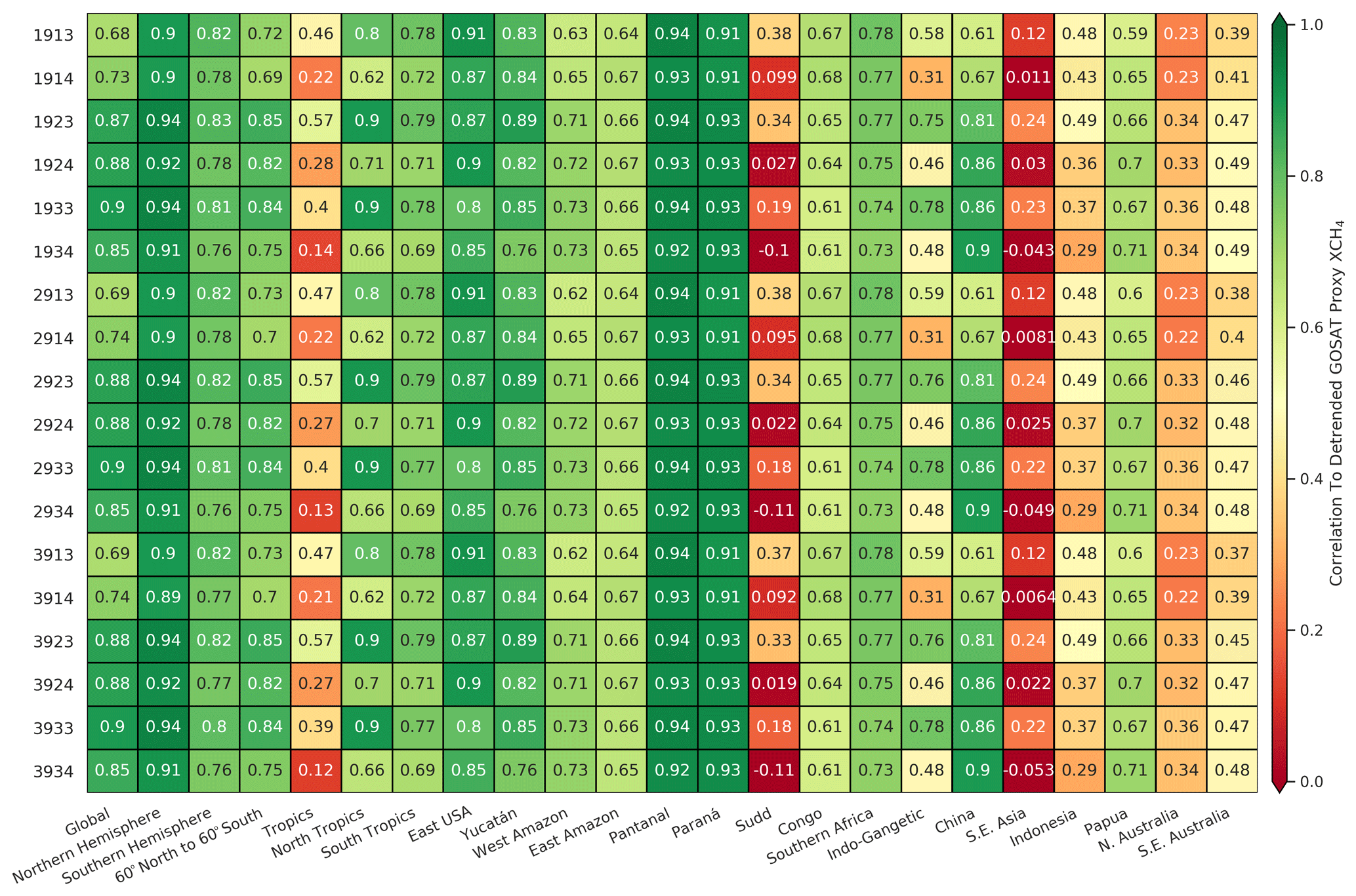
Figure A1Table showing the correlation coefficients between the modelled and observed seasonal cycle for all regions for every ensemble member.
The importance of the wetland extent parametrisation is region-specific, with the correlation to observations for the Tropics (especially the North Tropics) being much better for GLWD extent (0.80–0.90 for North Tropics) vs. GlobCover extent (0.62–0.71). Some regions are largely unaffected by the extent parametrisation in terms of their seasonality (e.g. West Amazon, East Amazon, Pantanal, Paraná, Congo), whilst some regions are significantly affected (e.g. Sudd, Indo-Gangetic, SE Asia).
The latest version of the University of Leicester GOSAT Proxy v9.0 XCH4 data (Parker and Boesch, 2020) is available from the Centre for Environmental Data Analysis data repository at https://doi.org/10.5285/18ef8247f52a4cb6a14013f8235cc1eb. The version used in this work (v7.2) is available via contacting the author. WetCHARTs v1.0 is available from Bloom et al. (2017a). This study uses v1.2.1 which is available on request from A. Anthony Bloom.
RJP generated the GOSAT XCH4 retrievals, performed the analysis and wrote the manuscript. AAB produced an updated version of the WetCHARTs dataset for use in this study. CW and MPC produced the TOMCAT model simulations. All co-authors contributed to the planning and discussion of this study and to refining the manuscript.
The authors declare that they have no conflict of interest.
Robert J. Parker, Hartmut Boesch, Chris Wilson and Martyn P. Chipperfield are funded via the UK National Centre for Earth Observation (NE/R016518/1 and NE/N018079/1). Joe McNorton acknowledges financial support from the Horizon 2020 CHE project (776186). We acknowledge the support of the UK Natural Environment Research Council through the grant The Global Methane Budget (MOYA, NE/N015681/1, NE/N015657/1 and NE/N015746/1). Part of this research was carried out at the Jet Propulsion Laboratory, California Institute of Technology, under a contract with the National Aeronautics and Space Administration. Funding for the WetCHARTs emissions was provided through a NASA Carbon Monitoring System grant NNH14ZDA001N-CMS. We also acknowledge funding from the ESA GHG-CCI and Copernicus C3S projects.
We thank the Japanese Aerospace Exploration Agency, National Institute for Environmental Studies and the Ministry of the Environment for the GOSAT data and their continuous support as part of the Joint Research Agreement. This research used the ALICE high-performance-computing facility at the University of Leicester for the GOSAT retrievals and analysis. The TOMCAT simulations were performed on the national ARCHER and Leeds ARC HPC systems.
The MODIS Surface Reflectance 8-Day L3 data and MODIS Combined 16-Day NDWI data were visualised via the Google Earth Engine software with the data provided courtesy of the NASA EOSDIS Land Processes Distributed Active Archive Center (LP DAAC), USGS Earth Resources Observation and Science (EROS) Center, Sioux Falls, South Dakota (https://lpdaac.usgs.gov, last access: 12 November 2020).
This research has been supported by the Natural Environment Research Council (grant nos. NE/R016518/1, NE/N018079/1, NE/N015681/1, NE/N015657/1 and NE/N015746/1), the National Aeronautics and Space Administration (grant no. NNH14ZDA001N-CMS), and the Horizon 2020 CHE project (grant no. 776186).
This paper was edited by Alexey V. Eliseev and reviewed by two anonymous referees.
Alexe, M., Bergamaschi, P., Segers, A., Detmers, R., Butz, A., Hasekamp, O., Guerlet, S., Parker, R., Boesch, H., Frankenberg, C., Scheepmaker, R. A., Dlugokencky, E., Sweeney, C., Wofsy, S. C., and Kort, E. A.: Inverse modelling of CH4 emissions for 2010–2011 using different satellite retrieval products from GOSAT and SCIAMACHY, Atmos. Chem. Phys., 15, 113–133, https://doi.org/10.5194/acp-15-113-2015, 2015. a
Becker, M., Papa, F., Frappart, F., Alsdorf, D., Calmant, S., da Silva, J. S., Prigent, C., and Seyler, F.: Satellite-based estimates of surface water dynamics in the Congo River Basin, Int. J. Appl. Earth Obs., 66, 196–209, https://doi.org/10.1016/j.jag.2017.11.015, 2018. a
Berchet, A., Pison, I., Chevallier, F., Paris, J.-D., Bousquet, P., Bonne, J.-L., Arshinov, M. Y., Belan, B. D., Cressot, C., Davydov, D. K., Dlugokencky, E. J., Fofonov, A. V., Galanin, A., Lavrič, J., Machida, T., Parker, R., Sasakawa, M., Spahni, R., Stocker, B. D., and Winderlich, J.: Natural and anthropogenic methane fluxes in Eurasia: a mesoscale quantification by generalized atmospheric inversion, Biogeosciences, 12, 5393–5414, https://doi.org/10.5194/bg-12-5393-2015, 2015. a
Bloom, A. A., Exbrayat, J. F., Van Der Velde, I. R., Feng, L., and Williams, M.: The decadal state of the terrestrial carbon cycle: Global retrievals of terrestrial carbon allocation, pools, and residence times, P. Natl. Acad. Sci. USA, 113, 1285–1290, https://doi.org/10.1073/pnas.1515160113, 2016. a
Bloom, A., Bowman, K., Lee, M., Turner, A., Schroeder, R., Worden, J., Weidner, R., Mcdonald, K., and Jacob, D.: CMS: Global 0.5-deg Wetland Methane Emissions and Uncertainty (WetCHARTs v1.0), ORNL DAAC, https://doi.org/10.3334/ORNLDAAC/1502, 2017a. a
Bloom, A. A., Bowman, K. W., Lee, M., Turner, A. J., Schroeder, R., Worden, J. R., Weidner, R., McDonald, K. C., and Jacob, D. J.: A global wetland methane emissions and uncertainty dataset for atmospheric chemical transport models (WetCHARTs version 1.0), Geosci. Model Dev., 10, 2141–2156, https://doi.org/10.5194/gmd-10-2141-2017, 2017b. a, b, c, d, e
Bohn, T. J., Melton, J. R., Ito, A., Kleinen, T., Spahni, R., Stocker, B. D., Zhang, B., Zhu, X., Schroeder, R., Glagolev, M. V., Maksyutov, S., Brovkin, V., Chen, G., Denisov, S. N., Eliseev, A. V., Gallego-Sala, A., McDonald, K. C., Rawlins, M. A., Riley, W. J., Subin, Z. M., Tian, H., Zhuang, Q., and Kaplan, J. O.: WETCHIMP-WSL: intercomparison of wetland methane emissions models over West Siberia, Biogeosciences, 12, 3321–3349, https://doi.org/10.5194/bg-12-3321-2015, 2015. a
Bontemps, S., Defourny, P., Bogaert, E. V., Arino, O., Kalogirou, V., and Perez, J. R.: GLOBCOVER 2009-Products Description and Validation Report, Tech. rep., available at: https://epic.awi.de/id/eprint/31014/16/GLOBCOVER2009_Validation_Report_2-2.pdf (last access: 12 November 2020), 2011. a
Buchwitz, M., Reuter, M., Schneising, O., Hewson, W., Detmers, R. G., Boesch, H., Hasekamp, O. P., Aben, I., Bovensmann, H., Burrows, J. P., Butz, A., Chevallier, F., Dils, B., Frankenberg, C., Heymann, J., Lichtenberg, G., De Mazière, M., Notholt, J., Parker, R., Warneke, T., Zehner, C., Griffith, D. W. T., Deutscher, N. M., Kuze, A., Suto, H., Wunch, D., Maziere, M. D., Notholt, J., Parker, R., Warneke, T., Zehner, C., Griffith, D. W. T., Deutscher, N. M., Kuze, A., Suto, H., and Wunch, D.: Global satellite observations of column-averaged carbon dioxide and methane: The GHG-CCI XCO2 and XCH4 CRDP3 data set, Remote Sens. Environ., 203, 276–295, https://doi.org/10.1016/j.rse.2016.12.027, 2017. a, b
Buchwitz, M., Reuter, M., Schneising, O., Bovensmann, H., Burrows, J. P., Boesch, H., Anand, J., Parker, R., Detmers, R. G., Aben, I., Hasekamp, O. P., Crevoisier, C., Armante, R., Zehner, C., and Schepers, D.: Copernicus Climate Change Service (C3S) global satellite observations of atmospheric carbon dioxide and methane, Proceedings of the International Astronautical Congress, IAC, 2018-October, 57–60, https://doi.org/10.1007/s42423-018-0004-6, 2018. a
Chipperfield, M. P.: New version of the TOMCAT/SLIMCAT off-line chemical transport model: Intercomparison of stratospheric tracer experiments, Q. J. Roy. Meteor. Soc., 132, 1179–1203, https://doi.org/10.1256/qj.05.51, 2006. a
Clark, D. B., Mercado, L. M., Sitch, S., Jones, C. D., Gedney, N., Best, M. J., Pryor, M., Rooney, G. G., Essery, R. L. H., Blyth, E., Boucher, O., Harding, R. J., Huntingford, C., and Cox, P. M.: The Joint UK Land Environment Simulator (JULES), model description – Part 2: Carbon fluxes and vegetation dynamics, Geosci. Model Dev., 4, 701–722, https://doi.org/10.5194/gmd-4-701-2011, 2011. a
Cogan, A. J., Boesch, H., Parker, R. J., Feng, L., Palmer, P. I., Blavier, J.-F. L. F., Deutscher, N. M., MacAtangay, R., Notholt, J., Roehl, C., Warneke, T., and Wunch, D.: Atmospheric carbon dioxide retrieved from the Greenhouse gases Observing SATellite (GOSAT): Comparison with ground-based TCCON observations and GEOS-Chem model calculations, J. Geophys. Res.-Atmos., 117, D21301, https://doi.org/10.1029/2012JD018087, 2012. a
Comyn-Platt, E., Hayman, G., Huntingford, C., Chadburn, S. E., Burke, E. J., Harper, A. B., Collins, W. J., Webber, C. P., Powell, T., Cox, P. M., Gedney, N., and Sitch, S.: Carbon budgets for 1.5 and 2 ∘C targets lowered by natural wetland and permafrost feedbacks, Nat. Geosci., 11, 568, https://doi.org/10.1038/s41561-018-0174-9, 2018. a
Cressot, C., Chevallier, F., Bousquet, P., Crevoisier, C., Dlugokencky, E. J., Fortems-Cheiney, A., Frankenberg, C., Parker, R., Pison, I., Scheepmaker, R. A., Montzka, S. A., Krummel, P. B., Steele, L. P., and Langenfelds, R. L.: On the consistency between global and regional methane emissions inferred from SCIAMACHY, TANSO-FTS, IASI and surface measurements, Atmos. Chem. Phys., 14, 577–592, https://doi.org/10.5194/acp-14-577-2014, 2014. a
Dadson, S. J., Ashpole, I., Harris, P., Davies, H. N., Clark, D. B., Blyth, E., and Taylor, C. M.: Wetland inundation dynamics in a model of land surface climate: Evaluation in the Niger inland delta region, J. Geophys. Res.-Atmos., 115, D23114, https://doi.org/10.1029/2010JD014474, 2010. a
Dee, D. P., Uppala, S. M., Simmons, A. J., Berrisford, P., Poli, P., Kobayashi, S., Andrae, U., Balmaseda, M. A., Balsamo, G., Bauer, P., Bechtold, P., Beljaars, A. C. M., van de Berg, L., Bidlot, J., Bormann, N., Delsol, C., Dragani, R., Fuentes, M., Geer, A. J., Haimberger, L., Healy, S. B., Hersbach, H., Hólm, E. V., Isaksen, L., Kållberg, P., Köhler, M., Matricardi, M., McNally, A. P., Monge-Sanz, B. M., Morcrette, J.-J., Park, B.-K., Peubey, C., de Rosnay, P., Tavolato, C., Thépaut, J.-N., and Vitart, F.: The ERA-Interim reanalysis: configuration and performance of the data assimilation system, Q. J. Roy. Meteor. Soc., 137, 553–597, https://doi.org/10.1002/qj.828, 2011. a, b
Dils, B., Buchwitz, M., Reuter, M., Schneising, O., Boesch, H., Parker, R., Guerlet, S., Aben, I., Blumenstock, T., Burrows, J. P., Butz, A., Deutscher, N. M., Frankenberg, C., Hase, F., Hasekamp, O. P., Heymann, J., De Mazière, M., Notholt, J., Sussmann, R., Warneke, T., Griffith, D., Sherlock, V., and Wunch, D.: The Greenhouse Gas Climate Change Initiative (GHG-CCI): comparative validation of GHG-CCI SCIAMACHY/ENVISAT and TANSO-FTS/GOSAT CO2 and CH4 retrieval algorithm products with measurements from the TCCON, Atmos. Meas. Tech., 7, 1723–1744, https://doi.org/10.5194/amt-7-1723-2014, 2014. a, b
Eliseev, A. V., Mokhov, I. I., Arzhanov, M. M., Demchenko, P. F., and Denisov, S. N.: Interaction of the methane cycle and processes in wetland ecosystems in a climate model of intermediate complexity, Izvestiya – Atmospheric and Ocean Physics, 44, 139–152, https://doi.org/10.1134/S0001433808020011, 2008. a
Feng, L., Palmer, P. I., Bösch, H., Parker, R. J., Webb, A. J., Correia, C. S. C., Deutscher, N. M., Domingues, L. G., Feist, D. G., Gatti, L. V., Gloor, E., Hase, F., Kivi, R., Liu, Y., Miller, J. B., Morino, I., Sussmann, R., Strong, K., Uchino, O., Wang, J., and Zahn, A.: Consistent regional fluxes of CH4 and CO2 inferred from GOSAT proxy XCH4 : XCO2 retrievals, 2010–2014, Atmos. Chem. Phys., 17, 4781–4797, https://doi.org/10.5194/acp-17-4781-2017, 2017. a
Fraser, A., Palmer, P. I., Feng, L., Boesch, H., Cogan, A., Parker, R., Dlugokencky, E. J., Fraser, P. J., Krummel, P. B., Langenfelds, R. L., O'Doherty, S., Prinn, R. G., Steele, L. P., van der Schoot, M., and Weiss, R. F.: Estimating regional methane surface fluxes: the relative importance of surface and GOSAT mole fraction measurements, Atmos. Chem. Phys., 13, 5697–5713, https://doi.org/10.5194/acp-13-5697-2013, 2013. a
Ganesan, A. L., Rigby, M., Lunt, M. F., Parker, R. J., Boesch, H., Goulding, N., Umezawa, T., Zahn, A., Chatterjee, A., Prinn, R. G., Tiwari, Y. K., Van Der Schoot, M., and Krummel, P. B.: Atmospheric observations show accurate reporting and little growth in India's methane emissions, Nat. Commun., 8, 836, https://doi.org/10.1038/s41467-017-00994-7, 2017. a
Ganesan, A. L., Schwietzke, S., Poulter, B., Arnold, T., Lan, X., Rigby, M., Vogel, F. R., van der Werf, G. R., Janssens-Maenhout, G., Boesch, H., Pandey, S., Manning, A. J., Jackson, R. B., Nisbet, E. G., and Manning, M. R.: Advancing Scientific Understanding of the Global Methane Budget in Support of the Paris Agreement, Global Biogeochem. Cy., 33, 1475–1512, https://doi.org/10.1029/2018GB006065, 2019. a
Gedney, N., Cox, P. M., and Huntingford, C.: Climate feedback from wetland methane emissions, Geophys. Res. Lett., 31, L20503, https://doi.org/10.1029/2004GL020919, 2004. a
Huntzinger, D. N., Schwalm, C., Michalak, A. M., Schaefer, K., King, A. W., Wei, Y., Jacobson, A., Liu, S., Cook, R. B., Post, W. M., Berthier, G., Hayes, D., Huang, M., Ito, A., Lei, H., Lu, C., Mao, J., Peng, C. H., Peng, S., Poulter, B., Riccuito, D., Shi, X., Tian, H., Wang, W., Zeng, N., Zhao, F., and Zhu, Q.: The North American Carbon Program Multi-Scale Synthesis and Terrestrial Model Intercomparison Project – Part 1: Overview and experimental design, Geosci. Model Dev., 6, 2121–2133, https://doi.org/10.5194/gmd-6-2121-2013, 2013. a
Kirschke, S., Bousquet, P., Ciais, P., et al.: Three decades of global methane sources and sinks, Nat. Geosci., 6, 813–823, https://doi.org/10.1038/ngeo1955, 2013. a
Kleinen, T., Brovkin, V., and Schuldt, R. J.: A dynamic model of wetland extent and peat accumulation: results for the Holocene, Biogeosciences, 9, 235–248, https://doi.org/10.5194/bg-9-235-2012, 2012. a
Lee, H., Beighley, R. E., Alsdorf, D., Jung, H. C., Shum, C. K., Duan, J., Guo, J., Yamazaki, D., and Andreadis, K.: Characterization of terrestrial water dynamics in the Congo Basin using GRACE and satellite radar altimetry, Remote Sens. Environ., 115, 3530–3538, https://doi.org/10.1016/j.rse.2011.08.015, 2011. a
Lehner, B. and Döll, P.: Development and validation of a global database of lakes, reservoirs and wetlands, J. Hydrol., 296, 1–22, https://doi.org/10.1016/j.jhydrol.2004.03.028, 2004. a, b
Lunt, M. F., Palmer, P. I., Feng, L., Taylor, C. M., Boesch, H., and Parker, R. J.: An increase in methane emissions from tropical Africa between 2010 and 2016 inferred from satellite data, Atmos. Chem. Phys., 19, 14721–14740, https://doi.org/10.5194/acp-19-14721-2019, 2019. a, b, c, d, e, f
Maasakkers, J. D., Jacob, D. J., Sulprizio, M. P., Scarpelli, T. R., Nesser, H., Sheng, J.-X., Zhang, Y., Hersher, M., Bloom, A. A., Bowman, K. W., Worden, J. R., Janssens-Maenhout, G., and Parker, R. J.: Global distribution of methane emissions, emission trends, and OH concentrations and trends inferred from an inversion of GOSAT satellite data for 2010–2015, Atmos. Chem. Phys., 19, 7859–7881, https://doi.org/10.5194/acp-19-7859-2019, 2019. a, b, c, d, e
McNorton, J., Gloor, E., Wilson, C., Hayman, G. D., Gedney, N., Comyn-Platt, E., Marthews, T., Parker, R. J., Boesch, H., and Chipperfield, M. P.: Role of regional wetland emissions in atmospheric methane variability, Geophys. Res. Lett., 43, 11433–11444, https://doi.org/10.1002/2016GL070649, 2016. a
Melton, J. R., Wania, R., Hodson, E. L., Poulter, B., Ringeval, B., Spahni, R., Bohn, T., Avis, C. A., Beerling, D. J., Chen, G., Eliseev, A. V., Denisov, S. N., Hopcroft, P. O., Lettenmaier, D. P., Riley, W. J., Singarayer, J. S., Subin, Z. M., Tian, H., Zürcher, S., Brovkin, V., van Bodegom, P. M., Kleinen, T., Yu, Z. C., and Kaplan, J. O.: Present state of global wetland extent and wetland methane modelling: conclusions from a model inter-comparison project (WETCHIMP), Biogeosciences, 10, 753–788, https://doi.org/10.5194/bg-10-753-2013, 2013. a, b
Olivier, J. G., Peters, J. A., and Janssens-Maenhout, G.: Trends in Global CO2 Emissions 2012 Report. PBL Netherlands Environmental Assessment Agency, Hague, the Netherlands, 2012. a
Parker, R. and Boesch, H.: University of Leicester GOSAT Proxy XCH4 v9.0, Centre for Environmental Data Analysis, https://doi.org/10.5285/18ef8247f52a4cb6a14013f8235cc1eb, 2020. a
Parker, R., Boesch, H., Cogan, A., Fraser, A., Feng, L., Palmer, P. I., Messerschmidt, J., Deutscher, N., Griffith, D. W. T., Notholt, J., Wennberg, P. O., and Wunch, D.: Methane observations from the Greenhouse Gases Observing SATellite: Comparison to ground-based TCCON data and model calculations, Geophys. Res. Lett., 38, L15807, https://doi.org/10.1029/2011GL047871, 2011. a
Parker, R. J., Boesch, H., Byckling, K., Webb, A. J., Palmer, P. I., Feng, L., Bergamaschi, P., Chevallier, F., Notholt, J., Deutscher, N., Warneke, T., Hase, F., Sussmann, R., Kawakami, S., Kivi, R., Griffith, D. W. T., and Velazco, V.: Assessing 5 years of GOSAT Proxy XCH4 data and associated uncertainties, Atmos. Meas. Tech., 8, 4785–4801, https://doi.org/10.5194/amt-8-4785-2015, 2015. a, b
Parker, R. J., Boesch, H., McNorton, J., Comyn-Platt, E., Gloor, M., Wilson, C., Chipperfield, M. P., Hayman, G. D., and Bloom, A. A.: Evaluating year-to-year anomalies in tropical wetland methane emissions using satellite CH4 observations, Remote Sens. Environ., 211, 261–275, https://doi.org/10.1016/j.rse.2018.02.011, 2018. a, b, c, d
Parker, R. J., Webb, A., Boesch, H., Somkuti, P., Barrio Guillo, R., Di Noia, A., Kalaitzi, N., Anand, J., Bergamaschi, P., Chevallier, F., Palmer, P. I., Feng, L., Deutscher, N. M., Feist, D. G., Griffith, D. W. T., Hase, F., Kivi, R., Morino, I., Notholt, J., Oh, Y.-S., Ohyama, H., Petri, C., Pollard, D. F., Roehl, C., Sha, M. K., Shiomi, K., Strong, K., Sussmann, R., Te, Y., Velazco, V. A., Warneke, T., Wennberg, P. O., and Wunch, D.: A Decade of GOSAT Proxy Satellite CH4 Observations, Earth Syst. Sci. Data Discuss., https://doi.org/10.5194/essd-2020-114, in review, 2020. a, b, c
Patra, P. K., Houweling, S., Krol, M., Bousquet, P., Belikov, D., Bergmann, D., Bian, H., Cameron-Smith, P., Chipperfield, M. P., Corbin, K., Fortems-Cheiney, A., Fraser, A., Gloor, E., Hess, P., Ito, A., Kawa, S. R., Law, R. M., Loh, Z., Maksyutov, S., Meng, L., Palmer, P. I., Prinn, R. G., Rigby, M., Saito, R., and Wilson, C.: TransCom model simulations of CH4 and related species: linking transport, surface flux and chemical loss with CH4 variability in the troposphere and lower stratosphere, Atmos. Chem. Phys., 11, 12813–12837, https://doi.org/10.5194/acp-11-12813-2011, 2011. a
Pekel, J. F., Cottam, A., Gorelick, N., and Belward, A. S.: High-resolution mapping of global surface water and its long-term changes, Nature, 540, 418–422, https://doi.org/10.1038/nature20584, 2016. a
Poulter, B., Bousquet, P., Canadell, J. G., Ciais, P., Peregon, A., Saunois, M., Arora, V. K., Beerling, D. J., Brovkin, V., Jones, C. D., Joos, F., Gedney, N., Ito, A., Kleinen, T., Koven, C. D., McDonald, K., Melton, J. R., Peng, C., and Peng, S.: Global wetland contribution to 2000–2012 atmospheric methane growth rate dynamics, Environ. Res. Lett., 12, 094013, https://doi.org/10.1088/1748-9326/aa8391, 2017. a, b
Rebelo, L. M., Senay, G. B., and McCartney, M. P.: Flood pulsing in the Sudd wetland: Analysis of seasonal variations in inundation and evaporation in South Sudan, Earth Interact., 16, 1–19, https://doi.org/10.1175/2011EI382.1, 2012. a, b
Saunois, M., Bousquet, P., Poulter, B., Peregon, A., Ciais, P., Canadell, J. G., Dlugokencky, E. J., Etiope, G., Bastviken, D., Houweling, S., Janssens-Maenhout, G., Tubiello, F. N., Castaldi, S., Jackson, R. B., Alexe, M., Arora, V. K., Beerling, D. J., Bergamaschi, P., Blake, D. R., Brailsford, G., Brovkin, V., Bruhwiler, L., Crevoisier, C., Crill, P., Covey, K., Curry, C., Frankenberg, C., Gedney, N., Höglund-Isaksson, L., Ishizawa, M., Ito, A., Joos, F., Kim, H.-S., Kleinen, T., Krummel, P., Lamarque, J.-F., Langenfelds, R., Locatelli, R., Machida, T., Maksyutov, S., McDonald, K. C., Marshall, J., Melton, J. R., Morino, I., Naik, V., O'Doherty, S., Parmentier, F.-J. W., Patra, P. K., Peng, C., Peng, S., Peters, G. P., Pison, I., Prigent, C., Prinn, R., Ramonet, M., Riley, W. J., Saito, M., Santini, M., Schroeder, R., Simpson, I. J., Spahni, R., Steele, P., Takizawa, A., Thornton, B. F., Tian, H., Tohjima, Y., Viovy, N., Voulgarakis, A., van Weele, M., van der Werf, G. R., Weiss, R., Wiedinmyer, C., Wilton, D. J., Wiltshire, A., Worthy, D., Wunch, D., Xu, X., Yoshida, Y., Zhang, B., Zhang, Z., and Zhu, Q.: The global methane budget 2000–2012, Earth Syst. Sci. Data, 8, 697–751, https://doi.org/10.5194/essd-8-697-2016, 2016. a, b
Saunois, M., Stavert, A. R., Poulter, B., Bousquet, P., Canadell, J. G., Jackson, R. B., Raymond, P. A., Dlugokencky, E. J., Houweling, S., Patra, P. K., Ciais, P., Arora, V. K., Bastviken, D., Bergamaschi, P., Blake, D. R., Brailsford, G., Bruhwiler, L., Carlson, K. M., Carrol, M., Castaldi, S., Chandra, N., Crevoisier, C., Crill, P. M., Covey, K., Curry, C. L., Etiope, G., Frankenberg, C., Gedney, N., Hegglin, M. I., Höglund-Isaksson, L., Hugelius, G., Ishizawa, M., Ito, A., Janssens-Maenhout, G., Jensen, K. M., Joos, F., Kleinen, T., Krummel, P. B., Langenfelds, R. L., Laruelle, G. G., Liu, L., Machida, T., Maksyutov, S., McDonald, K. C., McNorton, J., Miller, P. A., Melton, J. R., Morino, I., Müller, J., Murguia-Flores, F., Naik, V., Niwa, Y., Noce, S., O'Doherty, S., Parker, R. J., Peng, C., Peng, S., Peters, G. P., Prigent, C., Prinn, R., Ramonet, M., Regnier, P., Riley, W. J., Rosentreter, J. A., Segers, A., Simpson, I. J., Shi, H., Smith, S. J., Steele, L. P., Thornton, B. F., Tian, H., Tohjima, Y., Tubiello, F. N., Tsuruta, A., Viovy, N., Voulgarakis, A., Weber, T. S., van Weele, M., van der Werf, G. R., Weiss, R. F., Worthy, D., Wunch, D., Yin, Y., Yoshida, Y., Zhang, W., Zhang, Z., Zhao, Y., Zheng, B., Zhu, Q., Zhu, Q., and Zhuang, Q.: The Global Methane Budget 2000–2017, Earth Syst. Sci. Data, 12, 1561–1623, https://doi.org/10.5194/essd-12-1561-2020, 2020. a, b
Sheng, J.-X., Jacob, D. J., Turner, A. J., Maasakkers, J. D., Benmergui, J., Bloom, A. A., Arndt, C., Gautam, R., Zavala-Araiza, D., Boesch, H., and Parker, R. J.: 2010–2016 methane trends over Canada, the United States, and Mexico observed by the GOSAT satellite: contributions from different source sectors, Atmos. Chem. Phys., 18, 12257–12267, https://doi.org/10.5194/acp-18-12257-2018, 2018. a, b
Stocker, B. D., Spahni, R., and Joos, F.: DYPTOP: a cost-efficient TOPMODEL implementation to simulate sub-grid spatio-temporal dynamics of global wetlands and peatlands, Geosci. Model Dev., 7, 3089–3110, https://doi.org/10.5194/gmd-7-3089-2014, 2014. a
Tathy, J. P., Cros, B., Delmas, R. A., Marenco, A., Servant, J., and Labat, M.: Methane emission from flooded forest in central Africa, J. Geophys. Res., 97, 6159–6168, https://doi.org/10.1029/90JD02555, 1992. a
Thoning, K. W., Tans, P. P., and Komhyr, W. D.: Atmospheric carbon dioxide at Mauna Loa Observatory: 2. Analysis of the NOAA GMCC data, 1974–1985, J. Geophys. Res.-Atmos., 94, 8549–8565, https://doi.org/10.1029/JD094iD06p08549, 1989. a
Tootchi, A., Jost, A., and Ducharne, A.: Multi-source global wetland maps combining surface water imagery and groundwater constraints, Earth Syst. Sci. Data, 11, 189–220, https://doi.org/10.5194/essd-11-189-2019, 2019. a
Treat, C. C., Bloom, A. A., and Marushchak, M. E.: Nongrowing season methane emissions – a significant component of annual emissions across northern ecosystems, Glob. Change Biol., 24, 3331–3343, https://doi.org/10.1111/gcb.14137, 2018. a
Turner, A. J., Jacob, D. J., Benmergui, J., Wofsy, S. C., Maasakkers, J. D., Butz, A., Hasekamp, O., and Biraud, S. C.: A large increase in U.S. methane emissions over the past decade inferred from satellite data and surface observations, Geophys. Res. Lett., 43, 2218–2224, https://doi.org/10.1002/2016GL067987, 2016. a
Vallat, R.: Pingouin: statistics in Python, Journal of Open Source Software, 3, 1026, https://doi.org/10.21105/joss.01026, 2018. a
van der Werf, G. R., Randerson, J. T., Giglio, L., van Leeuwen, T. T., Chen, Y., Rogers, B. M., Mu, M., van Marle, M. J. E., Morton, D. C., Collatz, G. J., Yokelson, R. J., and Kasibhatla, P. S.: Global fire emissions estimates during 1997–2016, Earth Syst. Sci. Data, 9, 697–720, https://doi.org/10.5194/essd-9-697-2017, 2017. a
Webb, A. J., Bösch, H., Parker, R. J., Gatti, L. V., Gloor, E., Palmer, P. I., Basso, L. S., Chipperfield, M. P., Correia, C. S. C., Domingues, L. G., Feng, L., Gonzi, S., Miller, J. B., Warneke, T., and Wilson, C.: CH4 concentrations over the Amazon from GOSAT consistent with in situ vertical profile data, J. Geophys. Res.-Atmos., 121, 11006–11020, https://doi.org/10.1002/2016JD025263, 2016. a
Wilson, C., Chipperfield, M. P., Gloor, M., Parker, R. J., Boesch, H., McNorton, J., Gatti, L. V., Miller, J. B., Basso, L. S., and Monks, S. A.: Large and increasing methane emissions from Eastern Amazonia derived from satellite data, 2010–2018, Atmos. Chem. Phys. Discuss., https://doi.org/10.5194/acp-2020-1136, in review, 2020. a
Wunch, D., Toon, G. C., Wennberg, P. O., Wofsy, S. C., Stephens, B. B., Fischer, M. L., Uchino, O., Abshire, J. B., Bernath, P., Biraud, S. C., Blavier, J.-F. L., Boone, C., Bowman, K. P., Browell, E. V., Campos, T., Connor, B. J., Daube, B. C., Deutscher, N. M., Diao, M., Elkins, J. W., Gerbig, C., Gottlieb, E., Griffith, D. W. T., Hurst, D. F., Jiménez, R., Keppel-Aleks, G., Kort, E. A., Macatangay, R., Machida, T., Matsueda, H., Moore, F., Morino, I., Park, S., Robinson, J., Roehl, C. M., Sawa, Y., Sherlock, V., Sweeney, C., Tanaka, T., and Zondlo, M. A.: Calibration of the Total Carbon Column Observing Network using aircraft profile data, Atmos. Meas. Tech., 3, 1351–1362, https://doi.org/10.5194/amt-3-1351-2010, 2010. a
Wunch, D., Toon, G. C., Blavier, J.-F. L., Washenfelder, R. A., Notholt, J., Connor, B. J., Griffith, D. W. T., Sherlock, V., and Wennberg, P. O.: The Total Carbon Column Observing Network, Philos. T. R. S.-A, 369, 2087–2112, https://doi.org/10.1098/rsta.2010.0240, 2011. a, b
Xu, X., Yuan, F., Hanson, P. J., Wullschleger, S. D., Thornton, P. E., Riley, W. J., Song, X., Graham, D. E., Song, C., and Tian, H.: Reviews and syntheses: Four decades of modeling methane cycling in terrestrial ecosystems, Biogeosciences, 13, 3735–3755, https://doi.org/10.5194/bg-13-3735-2016, 2016. a
Yan, X., Akiyama, H., Yagi, K., and Akimoto, H.: Global estimations of the inventory and mitigation potential of methane emissions from rice cultivation conducted using the 2006 Intergovernmental Panel on Climate Change Guidelines, Global Biogeochem. Cy., 23, GB2002, https://doi.org/10.1029/2008GB003299, 2009. a
Zhang, B., Tian, H., Lu, C., Chen, G., Pan, S., Anderson, C., and Poulter, B.: Methane emissions from global wetlands: An assessment of the uncertainty associated with various wetland extent data sets, Atmos. Environ., 165, 310–321, https://doi.org/10.1016/j.atmosenv.2017.07.001, 2017. a
Zhang, Z., Zimmermann, N. E., Stenke, A., Li, X., Hodson, E. L., Zhu, G., Huang, C., and Poulter, B.: Emerging role of wetland methane emissions in driving 21st century climate change, P. Natl. Acad. Sci. USA, 114, 9647–9652, https://doi.org/10.1073/pnas.1618765114, 2017. a
- Abstract
- Introduction
- The WetCHARTs ensemble
- TOMCAT model simulations
- GOSAT Proxy XCH4 data
- Global evaluation of WetCHARTs
- Regional evaluation of WetCHARTs
- Case study 1 – the Paraná River
- Case study 2 – the Congo
- Case study 3 – Sudd
- Case study 4 – Yucatán
- Discussion and conclusions
- Appendix A: Regional correlation coefficients
- Data availability
- Author contributions
- Competing interests
- Acknowledgements
- Financial support
- Review statement
- References