Identifying Optimal Security Management Policy for Water–Energy–Food Nexus System under Stochastic and Fuzzy Conditions

Abstract

An interval-stochastic-fuzzy policy analysis model is proposed to generate optimal security management policy for a water–energy–food nexus system of the urban agglomeration under multiple uncertainties. A number of planning policies under interval-stochastic surface water and groundwater conditions are obtained. Ranking scores of all policies in descending order, policy with the highest score is the best choice. Results disclose that (a) interval-stochastic available water resources lead to changing system benefits. (b) The shares of cropland area targets are 2.7% (Xiamen), 42.6% (Zhangzhou), and 54.7% (Quanzhou). (c) Different available water scenarios result in varied irrigation patterns. (d) Surface water takes a high fraction of the total water supply (about [71.34, 73.68]%), diesel agricultural machinery service more than 60% of the total cropland. (e) Zhangzhou contributes about 50.01% of total TN and TP emissions, while Quanzhou contributes about 50.61% of total carbon emission. (f) Security level of policies would change with the varied σ and α values, due to the risk attitudes of policy makers. (h) Sweet potato and others are the crops with the highest safety performance; (i) Zhangzhou is the city with highest comprehensive safety performance.

1. Introduction

The water–energy–food nexus system represents a method to enhance the security and efficient management taking the inherent interactions into account [1]. Water is needed to make crops grow; electricity is required to collect, deliver, and treat water; energy (including electricity) is essential for harvesting and processing food; electricity generation needs water to cool machines; food waste can provide raw material for biomass energy [2,3,4]. Increasing resource interlinks due to growing scarcities, resources supply crises, and failures of sector-driven management strategies justified the need for the cross-sectoral integration of the resources [5]. Cities are sites of resources distribution, consumption, production, and recycling. A city often takes advantage of resources outside the city boundary, and then generates adverse environmental impacts inside other borders of cities. The idea behind the nexus is to look at the interdependent resource issues of water, energy, and food using an integrated framework in scientific analysis and policymaking. It is important to encompass the relationship between different resources in different cities, which formulate intricate water–energy–food nexus (WEF) systems. Global WEF securities (e.g., improved WEF policies lead to adaptive ecosystem and resource governance and management, in turn achieving sustainability outcomes) are facing unprecedented challenges from the fast speed of urbanization, increment of food demands, shortage of water resources, exhaustion of fossil energy, change of consumption patterns, competition over natural resources, attack of disasters, and impact of climate change [6,7]. Planning WEF systems in a security way which includes economic, social, and environmental development is the primary goal of policy makers.

Optimization models, running designed system models to obtain optimal results, are effective tools to gain insight into the complex WEF systems and provide policy making support for sustainable development [8]. Some researchers proposed models to manage the specific WEF systems. For instance, Leung Pah Hang [9] developed an WEF optimization model for a designated eco-town in the UK, where local water, food, and energy production systems were integrated into a framework. All possible planning policies (related to resources, productions, and wastes) were designed based on each supply subsystem and their interactions. Results disclosed that WEF systems were more resource efficient than individual systems. Si et al. [10] established a multiobjective WEF optimization model for the Upper Yellow River Basin (UYRB, in China), considering the benefits of water allocation, food cultivation, and hydropower utilization of reservoirs. The research revealed the WEF in the UYRB under multiple scenarios. The model showed the feasibility to be extended to other similar WEF systems worldwide. Sadeghi et al. [11] proposed an interdisciplinary WEF optimization model at the Shazand Watershed (in Iran) since related approaches were rarely practiced at the watershed scale. Maximum WEF index and optimal cropping pattern were obtained under conditions of determined consumption amount, mass productivity, and economic productivity of water and energy. Results were helpful to designate proper soil and water resource management strategies in the region. Guan et al. [12] quantified the WEF interactions in the metropolitan area of Phoenix (in Arizona, US), where many possible future scenarios about water–energy demand, water–energy supply, and food production were calculated as well as optimal policies were analyzed. This model could be transferable to other metropolitan regions since related applications were limited. Wu et al. [13] built a WEF optimization model that incorporated both supply and demands sides into a single system-of-systems model using the system dynamics approach. Through the case study of Saskatchewan (in Canada), the various levels of sensitivities of water, energy, and food sectors to the socioeconomic and climatic drivers were disclosed. The model allowed for socioeconomic and climatic scenario analysis toward integrated resources management, and its generic model structure could be expanded to other regions. Núñez-López et al. [14] developed a multiobjective optimization model that targeted economic and environmental objectives for the optimal design of a resilient WEF macroscopic system in the northwest part of Mexico. The model generated resilient solutions in satisfying water, energy, and food demands with an appropriate distribution of resources under the extreme climatic conditions. Chams et al. [15] presented an optimization model for WEF resource management and allocation at a regional scale. Policies under several resource availability scenarios and different targets were obtained. The model improved the understanding of the interlinkages among the nexus sectors by demonstrating the sensitivity of the WEF to adopted strategies. Generally, the above models (i) quantified the inherent interrelationships between system components, (ii) maximized system economic/environmental benefits subject to a number of social, economic, political, environmental, and physical constraints; (iii) provided policies associated with water and energy consumption, food production, and/or pollutant emission. Although these models provide a simple and practical methodology for large-scale problems, some of the generated policies may not be feasible and acceptable (due to the ignorance of risks existing in individual components; e.g., food productions, water supplies, and/or energy consumptions of a city).

Security assessment of individual components can help policy makers to select the acceptable and feasible policies as well as locate the points for improvement. Multicriteria decision making (MCDM) is a type of operational evaluation and decision support method, which is capable of handling complex issues featuring conflicting criteria, different data forms, multiple interests, and the explanation of evolving systems [16,17]. MCDM was extensively used in the field of water, food, or energy. For instance, Butchart-Kuhlmann et al. [18] assessed the water quantity in the Luanginga basin under various climate and land-use change scenarios, in which monthly flows, extreme low flows, high flow pulses, small floods, and large floods were selected as criteria. The research showed great potential for spatial analysis, resources management, and RCP/SSP coupling. Wang et al. [19] proposed a combined MCDM approach for the selection of ventilation heat recovery devices by using three different small buildings as examples. The method provided ideal guidance in choosing heat recovery devices based on buildings’ properties and policy makers’ preferences (e.g., investment cost, system performance, running cost, and space occupation). Zhu et al. [20] guided a risk-informed water resource decision in a reservoir operation problem, considering criteria of end water level, the peak discharge, downstream control point, the highest reservoir water level, and reservoir overtopping risk. The research framework enabled water managers to examine the robustness of final decisions and allowed the decisions to be made with higher reliabilities. Balezentis et al. [21] developed an integrated MCDM framework for estimating the cropping sustainability at the country (i.e., Lithuania) level. A number of sustainability criteria were used to rank the crop mixes policies. Optimal options for supporting crop farming sustainability were selected. Paul et al. [22] provided a MCDM framework to evaluate the potential of reclaimed water to irrigation (chosen State of California as study area), where multiple qualitative and quantitative decision criteria contained cropland, climate conditions, water policies, irrigation situations, and proximity to sewage treatment plants. The most influential criteria were identified. Rubio-Aliaga et al. [23] designed a multidimensional MCDM framework for a Spanish groundwater pumping system, where the optimal energy resources and water storage options were ordered and identified. The research provided scientifically supported groundwater pumping decision making processes. Arjomandi et al. [24] used MCDM method to determine the optimal land-use allocation according to the economic, social, and environmental criteria in the Hablehroud (in Iran) watershed. Effective recommendations were made to improve watershed management policies based on the optimal land-use patterns. These cases proved the feasibility of the MCDM approach in policy making processes. Very few studies demonstrated the application of the MCDA method for the WEF security management.

A real policy making system often features multiple uncertainties originated from variations of natural, social, economic, environmental conditions as well as internal relationships [25]. Interval two-stage stochastic programming (ITSP) can incorporate randomness and interval within the modeling processes; moreover, it can take recourse actions to cover the deficits due to the violation of plans pre-regulated by policy makers [26,27,28]. An ITSP model can be developed for generating holistic optimal WEF management policies. In addition, the fuzzy set theory that presents uncertainties in human ideas as well as interval that represents criteria with optimistic and pessimistic information, can be coupled with the MCDM approaches to get more sensitive, concrete, and realistic results [29]. An interval-fuzzy ordered weighted averaging operator (IF-OWA) method, belonging to MCDM methods, can be employed to assess the security level of the optimized system.

Through coupling the ITSP model and IF-OWA method, an interval-stochastic-fuzzy policy analysis (ISF-PA) model can be developed. The proposed model is applied a case study of the Xiamen-Zhangzhou-Quanzhou urban agglomeration (southeast of Fujian Province in south China). Results are expected to be helpful for identifying the urban agglomeration WEF security patterns.

2. Materials and Methods

2.1. Interval Two-Stage Stochastic Programming (ITSP)

In WEF management problems, uncertainties such as resources availability, economy fluctuation, and system security, should be taken into account. ITSP is an effective tool to handle issues where uncertainties are represented as probability distributions and interval numbers (parameters with lower- and upper-bounds), as well as scenario analyses are desired [30]. It merges local management policies into its optimization process and analyzes the policy of the preset targets with various economic penalty related situations [31]. A generalized ITSP can be presented as:

$$\mathrm{Max}{f}^{\pm }=C^{\pm }{X}^{\pm }+E_{{\omega }^{\pm }\in Q^{\pm }}[Q(X^{\pm },{\omega }^{\pm })]$$

(1)

Subject to:

$$A^{\pm }{X}^{\pm }\le B^{\pm }$$

(2)

$$Q(X^{\pm },{\omega }^{\pm })=\min q(Y^{\pm },{\omega }^{\pm })$$

(3)

$$T({\omega }^{\pm })X^{\pm }+W({\omega }^{\pm })Y^{\pm }\le H({\omega }^{\pm })$$

(4)

$$X^{\pm }\ge 0$$

(5)

$$Y^{\pm }\ge 0$$

(6)

where $X^{\pm }$ is first-stage decision variable (i.e., preset target); $Y^{\pm }$ is second-stage decision variable (i.e., occurred event); ${\omega }^{\pm }$ is random variable defined in probability space $({\Omega }^{\pm },F^{\pm },\mathrm{Pr})$; E is expectation values; $C^{\pm }$, $A^{\pm }$, and $B^{\pm }$ are known coefficient matrices, $T({\omega }^{\pm })$, $W({\omega }^{\pm })$, and $H({\omega }^{\pm })$ are functions of the random variable. The random variable can be discretized into a couple of certain interval values with associated probabilities to reflect the uncertainties [32]. The above ITSP can then be simplified as follows [33]:

$$\mathrm{Max}{f}^{\pm }={\displaystyle \sum _{j=1}^{n_1}{c}_j^{\pm }{x}_j^{\pm }}-{\displaystyle \sum _{j=1}^{n_2}{\displaystyle \sum _{h=1}^H{p}_h{e}_j^{\pm }{y}_{jh}^{\pm }}}$$

(7)

Subject to:

$${\displaystyle \sum _{j=1}^{n_1}{a}_{rj}^{\pm }{x}_j^{\pm }}\le b_r^{\pm }$$

(8)

$${\displaystyle \sum _{j=1}^{n_1}{a}_{rj}^{\pm }{x}_j^{\pm }}+{\displaystyle \sum _{j=1}^{n_2}{a}_{tj}^{\prime }{y}_{jh}^{\pm }}\ge {\stackrel{⌢}{\omega }}_h^{\pm }$$

(9)

$$x_j^{\pm }\ge 0$$

(10)

$$y_{jh}^{\pm }\ge 0$$

(11)

where ${\stackrel{⌢}{\omega }}_h^{\pm }$ is random variables with discrete probability level $p_h^{}$; $h=1,2,\dots ,H$ is the corresponding scenario. The ITSP model can be divided into two submodels as [34]:

Upper-bound submodel:

$$\mathrm{Max}{f}^{+}={\displaystyle \sum _{j=1}^{n_2}{c}_j^{+}(x_j^{-}+\mathsf{\Delta }{x}_j^{\pm }{u}_j^{})}-{\displaystyle \sum _{j=1}^{k_1}{\displaystyle \sum _{h=1}^v{p}_h{e}_j^{-}{y}_{jh}^{-}}}-{\displaystyle \sum _{j=k_1+1}^{n_2}{\displaystyle \sum _{h=1}^v{p}_h{e}_j^{-}{y}_{jh}^{+}}}$$

(12)

Subject to:

$${\displaystyle \sum _{j=1}^{n_1}|a_{rj}^{}{|}^{+}sign(a_{rj}^{+})(x_j^{-}+\mathsf{\Delta }{x}_j^{\pm }{u}_j^{})}\le b_r^{+}$$

(13)

$$\begin{array}{l}{\displaystyle \sum _{j=1}^{n_1}|a_{rj}^{}{|}^{+}sign(a_{rj}^{+})(x_j^{-}+\mathsf{\Delta }{x}_j^{\pm }{u}_j^{})}+{\displaystyle \sum _{j=1}^{k_1}|a_{tj}^{\prime }{|}^{+}sign(a_{tj}^{\prime +})y_{jh}^{-}}\\ {\displaystyle \sum _{j=k_1+1}^{n_1}|a_{tj}^{\prime }{|}^{-}sign(a_{tj}^{\prime -})y_{jh}^{+}}\ge {\stackrel{⌢}{\omega }}_h^{-}\end{array}$$

(14)

$$0\le u_j^{}\le 1$$

(15)

$$y_{jh}^{+}\ge 0$$

(16)

Lower-bound submodel:

$$\mathrm{Max}{f}^{-}={\displaystyle \sum _{j=1}^{n_2}{c}_j^{-}(x_j^{-}+\mathsf{\Delta }{x}_j^{\pm }{u}_j^{})}-{\displaystyle \sum _{j=1}^{k_1}{\displaystyle \sum _{h=1}^v{p}_h{e}_j^{+}{y}_{jh}^{+}}}-{\displaystyle \sum _{j=k_1+1}^{n_2}{\displaystyle \sum _{h=1}^v{p}_h{e}_j^{+}{y}_{jh}^{+}}}$$

(17)

Subject to:

$${\displaystyle \sum _{j=1}^{n_1}|a_{rj}^{}{|}^{-}sign(a_{rj}^{-})(x_j^{-}+\mathsf{\Delta }{x}_j^{\pm }{u}_{j\mathrm{opt}}^{})}\le b_r^{-}$$

(18)

$$\begin{array}{l}{\displaystyle \sum _{j=1}^{n_1}|a_{rj}^{}{|}^{-}sign(a_{rj}^{+})(x_j^{-}+\mathsf{\Delta }{x}_j^{\pm }{u}_{j\mathrm{opt}}^{})}+{\displaystyle \sum _{j=1}^{k_1}|a_{tj}^{\prime }{|}^{-}sign(a_{tj}^{\prime -})y_{jh}^{+}}\\ {\displaystyle \sum _{j=k_1+1}^{n_1}|a_{tj}^{\prime }{|}^{+}sign(a_{tj}^{\prime +})y_{jh}^{-}}\ge {\stackrel{⌢}{\omega }}_h^{+}\end{array}$$

(19)

$$y_{jh}^{+}\ge y_{jh\mathrm{opt}}^{-},j=1,2,\dots ,k_2$$

(20)

$$y_{jh}^{-}\ge y_{jh\mathrm{opt}}^{+},j=k_2+1,k_2+2,\dots ,n_1$$

(21)

Through solving submodels, $[x_{j\mathrm{opt}}^{-},x_{j\mathrm{opt}}^{+}]$, $[y_{jh\mathrm{opt}}^{-},y_{jh\mathrm{opt}}^{+}]$, and $[f_{\mathrm{opt}}^{-},f_{\mathrm{opt}}^{+}]$ can be generated. Corresponding management policies related to water, energy, and food can then be obtained.

2.2. Interval-Fuzzy Ordered Weighted Averaging Operator (IF-OWA)

For achieving more reasonable management policies, further analysis is needed from the perspective of multiple conflicting criteria (e.g., benefit, cost, pollutant, labor, and resource). IF-OWA is used for conducting policy analysis. IF-OWA can assess the system under a series of criteria, which is helpful for managers to select an optimal scheme based on their risk attitudes. There are two key factors in the assessing system: the criteria important degrees and corresponding quantified estimated objectives [35]. The first factor is often expressed as linguistic variables based on experts’ subjective consciousness. The second factor is generally known to fall within a certain interval [36]. The method adopts fuzzy logic approach to handle the linguistic information and takes interval theory to dispose the estimated objectives. The solution process includes reordering the inputs in descending order, determining the weighting vector, and aggregative procedure.

The first step is to handle all criteria to formulate new inputs. This step needs to be conducted after obtaining detailed data of all criteria (i.e., results of the ITSP model). The estimated criteria are presented as interval numbers [37]:

$$x_{ij}^{\pm }=[x_{ij}^{-},x_{ij}^{+}]=\{\begin{array}{l}\alpha x_{ij}^{+}+(1-\alpha )x_{ij}^{-},\mathrm{for}\mathrm{positive}\mathrm{inputs}\\ \alpha x_{ij}^{-}+(1-\alpha )x_{ij}^{+},\mathrm{for}\mathrm{negative}\mathrm{inputs}\end{array};\forall i\le n,j\le m$$

(22)

where $x^{+}$ and $x^{-}$ represent the optimistic and pessimistic data for the positive criterion, and vice versa. $\alpha \in [0,1]$ represents the optimism degree of the decision maker, a higher $\alpha$ corresponds to a more optimistic attitude of the decision maker. Since all criteria have different units, they are necessary to be normalized as follows:

$$x_{ij}^{*}=\{\begin{array}{l}(x_{ij}-x_i^{\min })/(x_i^{\max }-x_i^{\min }),\mathrm{for}\mathrm{positive}\mathrm{inputs}\\ (x_i^{\max }-x_{ij})/(x_i^{\max }-x_i^{\min }),\mathrm{for}\mathrm{negative}\mathrm{inputs}\end{array};\forall i\le n,j\le m$$

(23)

where $x_i^{\max }$ and $x_i^{\min }$ are the maximum and the minimum values in criterion i, respectively. The new inputs can be obtained through multiplying $x_{ij}^{*}$ by normalized crisp data of important degree.

Five important degrees (d) are selected as unimportant, marginal important, moderate important, quite important, and extremely important. They are expressed as triangular fuzzy members, and transformed as normalized triangular fuzzy members [38]. For example, for moderate important degree, the normalized triangular fuzzy number is Z (0.50, 0.25, 0.25), the membership degree is f_z(0.50) = 1, and the left- and right-benchmarks of 0.50 are 0.25 and 0.25. Center of gravity method is then adopted to convert the normalized triangular fuzzy number into crisp data (i.e., (0.25 + 0.50 + 0.75) / 3 = 0.50). Exact values of important degrees are obtained. The normalized fuzzy members of five important degrees are 0.13, 0.25, 0.50, 0.75, and 0.87.

The next step is to identify weighting vectors of all criteria. Different σ (σ $\in$ [0, 1]) values denote deferent satisfactions to criteria considered in the decision-making system. σ = 0 means that only the minimal element in the inputs can be satisfied, and σ = 1 denotes that only the maximal element in the inputs can be satisfied. The weighting vector can be calculated as follows [39]:

$$w_1^{}=[2(2n-1)-6(n-1)(1-\sigma )]/[n(n+1)]$$

(24)

$$w_i^{}=[(n-i)(n-1)]/w_1+[(i-1)(n-1)]/w_n,\mathrm{if}i\in [2,\dots ,n-1]$$

(25)

$$w_n^{}=[6(n-1)(1-\sigma )-2(n-2)]/[n(n+1)]$$

(26)

The integrated score of an alternative policy can be calculated based on Equation (27). Ranking scores of all policies in descending order, the policy with the highest $F_j$ is the best choice:

$$F_j={\displaystyle \sum _{i=1}^n{w}_i{x}_{ij}^{*}{d}_i}$$

(27)

3. Case Study

3.1. Study Area Description

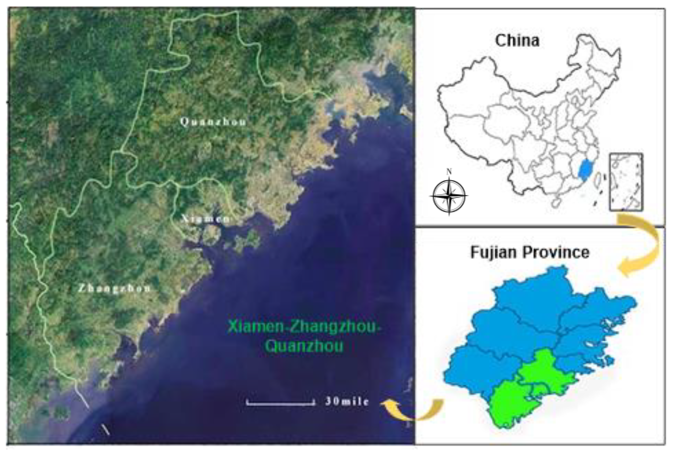
The Xiamen-Zhangzhou-Quanzhou urban agglomeration (24°28′55.77″ N–24°52′36.45″ N and 117°38′32.84″ E–118°40′16.72″ E) is located at southeast of Fujian Province in south China, with an area of approximately 25,314.17 km² (in Figure 1). It is one of the most important urban agglomerations in China, as well as the largest Metropolitan Area in Fujian Province in terms of both surface area and population (supported 51.4% of the provincial population and contributed 51.1% provincial population gross domestic products) [40,41,42,43,44]. The agglomeration is subjected to a typical subtropical ocean monsoon climate; the average annual rainfall is 1200–1800 mm, total annual solar radiation is 120–140 kcal/cm², and average temperature is about 19.5–21.0 °C. It contributes 18.46% of the total grain production with 33.64% of land area, 45.62% of cultivated land, 40.01% of water resources, and 37.81% of energy resources in the province [43].

Currently, expansion in urban capacity, variation in natural conditions, adjustment in land use, and fluctuation in resources demand lead to changing water–energy–food nexus structure of the agglomeration. For example, irrigation water keeps decreasing with a declined rate of 4.11%; cropland area keeps decreasing with a declined rate of 4.22%; fossil energy consumption keeps decreasing with a declined rate of 1.31%; electric energy keeps increasing with a growth rate of 3.72%; population keeps increasing with a growth rate of 7.33%; value-added rate of agriculture keeps decreasing with a declined rate of 1.81% [43]. Apparently, population growth leads to increasing food demand and electric energy (for daily life), low water resources first satisfy electricity generation and limited irrigation water supply; food should be imported from other regions, thus reduce the economic output. Decision makers pay much attention to the issues of making a reasonable cropland, water, and energy planning policy to satisfy water–energy–food nexus security, economic development, and environment requirement.

3.2. System Boundary and Components

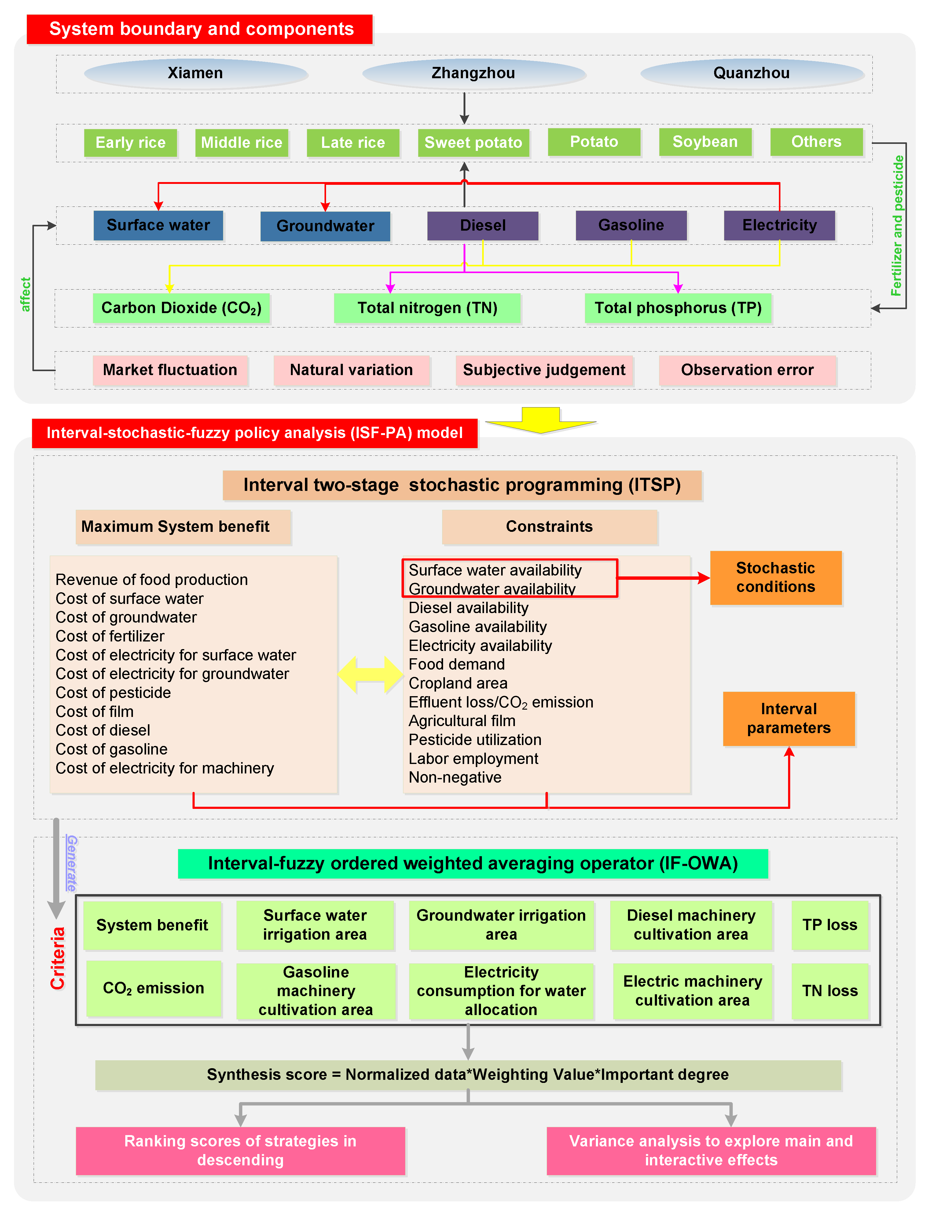
Urban agglomeration is a complex system consisting of social, economic, environmental, and resource factors. An interval-stochastic-fuzzy policy analysis (ISF-PA) model which couples ITSP and IF-OWA models is formulated to support WEF security under multiple uncertainties. The framework of the ISF-PA model is presented in Figure 2.

The study system is composed of (i) seven crops including early rice, middle rice, late rice, sweet potato, potato, soybean, and others; (ii) two water sources including surface water and groundwater; (iii) three energy sources including gasoline, diesel, and electricity; (iv) three emissions including carbon dioxide (CO₂), total phosphorus (TP), and total nitrogen (TN); (v) two chemicals: pesticide and fertilizer; (vi) three cities: Xiamen, Zhangzhou, Quanzhou. Decision making processes should fully consider market situation, water requirement and availability for irrigation, electricity demand for water collection and delivery, energy demand for machinery operation, energy availability, land use policy, effluent and carbon emission, labor employment, and food guarantee, as well as represent the complexities and interactions among them. Meanwhile, economic and technological parameters vary with market fluctuations, subjective judgments of experts affect data acquisition and system reliability, spatiotemporal variability of runoff leads to changed available water resources, food demand increases with population growth, arable land area and food types affect energy consumption. The uncertainties are quantified as interval, stochastic, and fuzzy variables.

3.3. Modelling Formulation

In the first stage, decision makers set initial targets of all crops in each city without catching available water resources conditions. In the second stage, random available water resources conditions are recognized. If targets are too high, local resources may not be sufficient to satisfy demand. Decision makers need to extract groundwater more deeply (which is harmful for aquifers). If targets are too low, local citizens may withstand economic losses. Infeasibilities in the second stage are allowed at a certain penalty (i.e., the second-stage decision is used to minimize penalty that may appear due to any infeasibility). A number of management policies related to cropland area, water allocation, and energy consumption can be obtained based on the ITSP model as follows:

Objective function:

$$\begin{array}{cc}\mathrm{Max}{f}^{\pm }& ={\displaystyle \sum _{c=1}^7{\displaystyle \sum _{s=1}^{3}M{P}_{c,s}^{\pm }(C{A}_{c,s}^{-}+\mathsf{\Delta }C{A}_{c,s}^{\pm }\cdot x_{c,s}^{})C{Y}_{c,s}^{\pm }}}-{\displaystyle \sum _{c=1}^7{\displaystyle \sum _{s=1}^3{\displaystyle \sum _{h_1=1}^3{p}_{h_1}^{sur}CS{W}_s^{\pm }CA{S}_{c,s,h_1}^{\pm }IQ{R}_c^{\pm }}}}\hfill \\ & -{\displaystyle \sum _{c=1}^7{\displaystyle \sum _{s=1}^3{\displaystyle \sum _{h_2=1}^3{p}_{h_2}^{gro}CG{W}_s^{\pm }CG{S}_{c,s,h_2}^{\pm }IQ{R}_c^{\pm }}}}-{\displaystyle \sum _{c=1}^7{\displaystyle \sum _{s=1}^{3}C{F}_s^{\pm }(C{A}_{c,s}^{-}+\mathsf{\Delta }C{A}_{c,s}^{\pm }{x}_{c,s}^{})}}\hfill \\ & -{\displaystyle \sum _{c=1}^7{\displaystyle \sum _{s=1}^3{\displaystyle \sum _{h=1}^3(p_{h_1}^{sur}C{E}_s^{\pm }CA{S}_{c,s,h}^{\pm }{}_{{}_1}UE{D}^{\pm }+p_{h_2}^{gro}CG{S}_{c,s,h_2}^{\pm }UE{G}^{\pm })IQ{R}_c^{\pm }}}}\hfill \\ & -{\displaystyle \sum _{c=1}^7{\displaystyle \sum _{s=1}^{3}C{P}_s^{\pm }(C{A}_{c,s}^{-}+\mathsf{\Delta }C{A}_{c,s}^{\pm }{x}_{c,s}^{})}}-{\displaystyle \sum _{c=1}^7{\displaystyle \sum _{s=1}^{3}CA{F}_s^{\pm }(C{A}_{c,s}^{-}+\mathsf{\Delta }C{A}_{c,s}^{\pm }{x}_{c,s}^{})}}\hfill \\ & -{\displaystyle \sum _{c=1}^7{\displaystyle \sum _{s=1}^{3}C{D}_s^{\pm }A{D}_{c,s}^{\pm }CD{A}_{c,s}^{\pm }}}-{\displaystyle \sum _{c=1}^7{\displaystyle \sum _{s=1}^{3}C{G}_s^{\pm }A{G}_{c,s}^{\pm }CG{A}_{c,s}^{\pm }}}-{\displaystyle \sum _{c=1}^7{\displaystyle \sum _{s=1}^3{\displaystyle \sum _{h=1}^{3}C{E}_s^{\pm }A{E}_s^{\pm }CE{A}_{c,s}^{\pm }}}}\hfill \end{array}$$

(28)

where c is index of crop; s is index of city; $h_1$ is available surface water level ($h_1=1$ for low, $h_1=2$ for medium, $h_1=3$ for high); $h_2$ is available groundwater level ($h_2=1$ for low, $h_2=2$ for medium, $h_2=3$ for high); $M{P}_{c,s}^{\pm }$ is market price (Yuan/kg); $C{A}_{c,s}^{-}$ is lower bound of cropland area target that should be irrigated by water and cultivated by energy agricultural machine (ha); $\mathsf{\Delta }C{A}_{c,s}^{\pm }$ is the difference between upper and lower bounds (ha); $x_{c,s}^{\pm }$ is decision variables for destemming cropland area target in first-stage; $C{Y}_{c,s}^{\pm }$ is unit crop yield (kg/ha); $p_h$ is probability of available water occurrence under level h; $CS{W}_s^{\pm }$ is unit cost of surface water (Yuan/m³); $CA{S}_{c,s,h}^{\pm }{}_{{}_1}$ is cropland area irrigated by surface water (ha); $IQ{R}_c^{\pm }$ is irrigation quota (m³/ha); $CG{W}_s^{\pm }$ is unit cost of groundwater (Yuan/m³); $CG{S}_{c,s,h}^{\pm }{}_{{}_2}$ is cropland area irrigated by groundwater (ha); $C{F}_s^{\pm }$ is unit cost of fertilizer (kg/ha); $C{P}_s^{\pm }$ is unit cost of pesticide (Yuan/kg); $CA{F}_s^{\pm }$ is unit cost of agricultural film (kg/ha); $C{D}_s^{\pm }$ is unit cost of diesel (Yuan/liter); $A{D}_{c,s}^{\pm }$ is unit diesel consumption of cropland (liter/ha); $CD{A}_{c,s}^{\pm }$ is cropland area cultivated by diesel agricultural machinery (ha); $CG{A}_{c,s}^{\pm }$ is cropland area cultivated by gasoline agricultural machinery (ha); $CE{A}_{c,s}^{\pm }$ is cropland area cultivated by electric agricultural machinery (ha); $C{G}_s^{\pm }$ is unit cost of gasoline (Yuan/liter); $A{G}_{c,s}^{\pm }$ is unit gasoline consumption of cropland (liter/ha); $C{E}_s^{\pm }$ is unit cost of electricity (Yuan/kWh); $A{E}_s^{\pm }$ is unit electricity consumption for cropland (kWh/ha); $UE{D}_{}^{\pm }$ is unit electricity consumption for surface water (kWh/m³); $UE{G}^{\pm }$ is unit electricity consumption for groundwater (kWh/m³);

Constraints:

(1) Surface water availability: Surface water delivered to all the crops in each city should not be higher than available surface water supply.

$${\displaystyle \sum _{c=1}^{7}CA{S}_{c,s,h_1}^{\pm }IQ{R}_c^{\pm }}\le AW{S}_{s,h_1}^{\pm }$$

(29)

(2) Groundwater availability: Groundwater allocated to all the crops in each city should not be higher than allowable groundwater pumping.

$${\displaystyle \sum _{c=1}^{7}CG{S}_{c,s,h}^{\pm }{}_{{}_2}IQ{R}_c^{\pm }}\le AG{W}_{s,h_2}^{\pm }$$

(30)

(3) Energy availability: The energy consumption for crop cultivation should not be higher than the available energy for agriculture in each subarea.

$${\displaystyle \sum _{c=1}^{7}A{D}_{c,s}^{\pm }CD{A}_{c,s}^{\pm }}\le AD{M}_s^{\pm }$$

(31)

$${\displaystyle \sum _{c=1}^{7}A{G}_{c,s}^{\pm }CG{A}_{c,s}^{\pm }\le AG{M}_s^{\pm }}$$

(32)

$${\displaystyle \sum _{c=1}^7[A{E}_s^{\pm }CE{A}_{c,s}^{\pm }}+(CA{S}_{c,s,h_1}^{\pm }UE{D}^{\pm }+CG{S}_{c,s,h_2}^{\pm }UE{G}^{\pm })IQ{R}_c^{\pm }]\le AE{M}_s^{\pm }$$

(33)

(4) Food security: The yield of food grain for each subarea should satisfy the food grain requirement that is associated with population in order to guarantee food security.

$${\displaystyle \sum _{c=1}^7(C{A}_{c,s}^{-}+\mathsf{\Delta }C{A}_{c,s}^{\pm }{x}_{c,s}^{})C{Y}_{c,s}^{\pm }}\ge P{P}_s^{\pm }\times F{D}_{}^{\pm }$$

(34)

(5) Cropland area: Cropland area should not be higher than the maximum value and lower than minimum value. All cropland should be irrigated by water and cultivated by energy agricultural machine.

$$C{A}_{c,s(\min )}^{\pm }\le C{A}_{c,s}^{-}+\mathsf{\Delta }C{A}_{c,s}^{\pm }{x}_{c,s}^{}\le C{A}_{c,s(\max )}^{\pm }$$

(35)

$$CG{S}_{c,s,h_1}^{\pm }+CA{S}_{c,s,h}^{\pm }{}_{{}_2}=C{A}_{c,s}^{-}+\mathsf{\Delta }C{A}_{c,s}^{\pm }{x}_{c,s}^{}$$

(36)

$$CD{A}_{c,s}^{\pm }+CG{A}_{c,s}^{\pm }+CE{A}_{c,s}^{\pm }=C{A}_{c,s}^{-}+\mathsf{\Delta }C{A}_{c,s}^{\pm }{x}_{c,s}^{}$$

(37)

(6) Total nitrogen emission: Nitrogen emission by fertilizer application should not be higher than the allowable amount.

$${\displaystyle \sum _{c=1}^7(C{A}_{c,s}^{-}+\mathsf{\Delta }C{A}_{c,s}^{\pm }{x}_{c,s}^{})F{A}_{c,s}^{\pm }N{C}_{}^{\pm }{\eta }_s^{\pm }\le TN{E}_s^{\pm }}$$

(38)

(7) Total phosphorus emission: Phosphorus emission by fertilizer application should not be higher than the allowable amount.

$${\displaystyle \sum _{c=1}^7(C{A}_{c,s}^{-}+\mathsf{\Delta }C{A}_{c,s}^{\pm }{x}_{c,s}^{})F{A}_{c,s}^{\pm }P{C}_{}^{\pm }{\lambda }_s^{\pm }\le TP{E}_s^{\pm }}$$

(39)

(8) Agricultural film utilization: Agricultural film utilization often causes plastic environmental pollution, which needs to be controlled.

$${\displaystyle \sum _{c=1}^7(C{A}_{c,s}^{-}+\mathsf{\Delta }C{A}_{c,s}^{\pm }{x}_{c,s}^{})F{U}_s^{\pm }\le TF{U}_s^{\pm }}$$

(40)

(9) Pesticide utilization: The spraying of pesticides often brings about COD and eutrophication environmental pollution, which must not exceed the allowable value.

$${\displaystyle \sum _{c=1}^7(C{A}_{c,s}^{-}+\mathsf{\Delta }C{A}_{c,s}^{\pm }{x}_{c,s}^{})\times P{U}_{c,s}^{\pm }\le TP{A}_s^{\pm }}$$

(41)

(10) Carbon emission: Excessive CO₂ emission can lead to greenhouse effect. It is important to control CO₂ emission.

$${\displaystyle \sum _{c=1}^7\left\{\begin{array}{l}A{D}_{c,s}^{\pm }{\alpha }_1^{\pm }+A{G}_{c,s}^{\pm }{\alpha }_2^{\pm }+A{E}_s^{\pm }{\alpha }_3^{\pm }\\ +F{A}_{c,s}^{\pm }{\alpha }_4^{\pm }+F{U}_s^{\pm }{\alpha }_5^{\pm }+P{U}_{c,s}^{\pm }{\alpha }_6^{\pm }\end{array}\right\}(C{A}_{c,s}^{-}+\mathsf{\Delta }C{A}_{c,s}^{\pm }{x}_{c,s}^{})}\le TC{E}_s^{\pm }$$

(42)

(11) Labor employment: The amount of labor is limited due to the budget.

$${\displaystyle \sum _{c=1}^7(C{A}_{c,s}^{-}+\mathsf{\Delta }C{A}_{c,s}^{\pm }{x}_{c,s}^{})LA{M}_s^{\pm }W{G}_{}^{\pm }}\le TW{G}_s^{\pm }$$

(43)

(12) Non-negative variable: Since this is a real-world case study, all variables should be non-negative. Through running the proposed model, solutions of all decision variables can be obtained. System benefit can then be determined.

$$0\le x_{c,s}^{\pm }\le 1$$

(44)

$$CG{S}_{c,s,h_1}^{\pm },CA{S}_{c,s,h}^{\pm }{}_{{}_2}\ge 0$$

(45)

$$CD{A}_{c,s}^{\pm },CG{A}_{c,s}^{\pm },CE{A}_{c,s}^{\pm }\ge 0$$

(46)

where $AW{S}_{s,h_1}^{\pm }$ is available surface water (m³); $AG{W}_{s,h_2}^{\pm }$ is available groundwater (m³); $AD{M}_s^{\pm }$ is available diesel supply (liter); $AG{M}_s^{\pm }$ is available gasoline supply (liter); $AE{M}_s^{\pm }$ is available electricity supply (kWh); $P{P}_s^{\pm }$ is number of population (person); $F{D}_{}^{\pm }$ is per food demand (kg/person); $C{A}_{c,s(\min )}^{\pm }$ is minimum cropland area (ha); $C{A}_{c,s(\max )}^{\pm }$ is maximum cropland area (ha); $F{A}_{c,s}^{\pm }$ is unit fertilizer application (kg/ha); $N{C}_{}^{\pm }$ is total nitrogen content of fertilizer (kg N/kg); ${\eta }_s^{\pm }$ is loss rate of total nitrogen (%); $TN{E}_s^{\pm }$ is allowable total nitrogen loss (kg N); $P{C}_{}^{\pm }$ is total phosphorus content of fertilizer (kg P/kg); ${\lambda }_s^{\pm }$ is loss rate of total phosphorus (%); $TP{E}_s^{\pm }$ is allowable total phosphorus loss (kg N); $F{U}_s^{\pm }$ is unit agricultural film application (kg/ha); $TF{U}_s^{\pm }$ is total allowable agricultural film application (t); $P{U}_{c,s}^{\pm }$ is unit pesticide application (kg/ha); $TP{A}_s^{\pm }$ is total allowable pesticide application (t); ${\alpha }_1^{\pm }$ is carbon emission of diesel (kgCO₂/ liter); ${\alpha }_2^{\pm }$ is carbon emission of gasoline (kgCO₂/ liter); ${\alpha }_3^{\pm }$ is carbon emission of electricity (kgCO₂/kg); ${\alpha }_4^{\pm }$ is carbon emission of fertilizer (kgCO₂/kg); ${\alpha }_5^{\pm }$ is carbon emission of film (kgCO₂/kg); ${\alpha }_6^{\pm }$ is carbon emission of pesticide (kgCO₂/kg); $TC{E}_s^{\pm }$ is total allowable carbon emission (kg); $LA{M}_s^{\pm }$ is number of labor (person/ha); $W{G}_{}^{\pm }$ is unit remuneration (Yuan/person); $TW{G}_s^{\pm }$ is total remuneration (Yuan).

Table 1. Values of interval parameters.

Parameter	City	Crop
		Early Rice	Middle Rice	Late Rice	Sweet Potato	Potato	Soybean	Others
Market price (Yuan/kg)	Xiamen	[2.81, 3.12]	[2.12, 2.36]	[2.22, 2.47]	[7.31, 8.12]	[2.11, 2.32]	[5.11, 5.68]	[14.11, 14.36]
	Zhangzhou	[2.71, 3.01]	[1.99, 2.22]	[2.01, 2.32]	[7.30, 8.01]	[1.95, 2.17]	[4.78, 5.33]	[12.61, 14.01]
	Quanzhou	[2.63, 2.97]	[1.95, 2.17]	[1.94, 2.16]	[7.17, 7.97]	[1.93, 2.14]	[4.61, 5.12]	[12.48, 13.87]
Crop yield (kg/ha)	Xiamen	[355, 395]	[275, 306]	[288, 320]	[377, 419]	[354, 394]	[161, 179]	[164, 183]
	Zhangzhou	[418, 465]	[390, 434]	[381, 424]	[441, 491]	[415, 462]	[254, 283]	[421, 468]
	Quanzhou	[360, 401]	[387, 430]	[348, 387]	[324, 360]	[238, 265]	[207, 231]	[319, 355]
Unit diesel consumption of cropland (liter/ha)	Xiamen	[10.97, 11.30]	[10.10, 10.41]	[10.83, 11.16]	[11.22, 11.55]	[10.76, 11.09]	[11.18, 11.52	[11.29, 11.63]
	Zhangzhou	[46.49, 47.88]	[46.04, 47.22]	[46.04, 47.42]	[45.95, 47.33]	[46.13, 47.52]	[45.69, 47.06]	[45.69, 47.06]
	Quanzhou	[31.84, 32.80]	[31.84, 32.80]	[31.84, 32.80]	[31.84, 32.80]	[31.84, 32.80]	[31.84, 32.80]	[31.84, 32.80]
Irrigation quota (m3/ha)	All	[266, 296]	[325, 337]	[339, 349]	[148, 155]	[148, 157]	[100, 108]	[219, 226]
Unit fertilizer application (kg/ha)	Xiamen	[38.79, 38.03]	[38.05, 38.81]	[38.06, 38.82]	[37.90, 38.66]	[37.76, 38.52]	[37.70, 38.45]	[37.58, 38.33]
	Zhangzhou	[67.00, 68.34]	[66.88, 68.21]	[66.88, 68.21]	[65.12, 66.43]	[64.38, 65.66]	[63.88, 65.15]	[62.5, 63.75]
	Quanzhou	[53.63, 54.70]	[53.13, 54.19]	[53.00, 54.06]	[52.75, 53.81]	[52.75, 53.81]	[52.13, 53.17]	[52.00, 53.04]
Unit pesticide application (kg/ha)	Xiamen	[2.35, 2.39]	[2.01, 2.05]	[1.92, 1.96]	[1.84, 1.88]	[1.98, 2.02]	[1.72, 1.75]	[1.76, 1.80]
	Zhangzhou	[3.61, 3.68]	[2.43, 2.48]	[2.15, 2.19]	[1.95, 2.06]	[2.03, 2.06]	[1.83, 1.87]	[1.82, 1.86]
	Quanzhou	[3.52, 3.60]	[2.34, 2.39]	[2.08, 2.12]	[1.89, 1.93]	[1.97, 2.01]	[1.81, 1.84]	[1.78, 1.82]

shows the interval values of different cities and crops. Market prices were obtained from the “Agricultural Product Price Information Network of Fujian Province”; Crop yields were gained from “Statistical Yearbook” of each city; irrigation quotas were obtained from “Standard Local Water Quota of Fujian Province”; unit diesel, fertilizer, and pesticide application were extracted from “Agricultural Information Network” of the cities. Other parameters were obtained from field research and published references [33,45,46].

Table 2. Stochastic surface water.

Scenario	Combination	Probability	Xiamen, Zhangzhou, and Quanzhou (106 m3)
Scenario 1 (S1)	$\begin{array}{l}(h_1=1,h_1=2,h_1=3,\\ h_2=1,h_2=2,h_2=3)\end{array}$	$\begin{array}{l}(0.23,0.56,0.21,\\ 0.18,0.57,0.25)\end{array}$	[100.4, 120.5], [154.9, 185.5], [182.0, 218.4]
			[240.0, 268.1], [271.8, 290.2], [291.0, 337.5]
			[287.3, 325.2], [344.8, 372.3], [386.0, 427.2]
Scenario 2 (S2)	$\begin{array}{l}(h_1=1,h_1=2,h_1=3,\\ h_2=1,h_2=3,h_2=2)\end{array}$	$\begin{array}{l}(0.23,0.56,0.21,\\ 0.18,0.25,0.57)\end{array}$	[100.4, 120.5], [154.9, 185.5], [182.0, 218.4]
			[240.0, 268.1], [271.8, 290.2], [291.0, 337.5]
			[287.3, 325.2], [344.8, 372.3], [386.0, 427.2]
Scenario 3 (S3)	$\begin{array}{l}(h_1=1,h_1=2,h_1=3,\\ h_2=2,h_2=1,h_2=3)\end{array}$	$\begin{array}{l}(0.23,0.56,0.21,\\ 0.57,0.18,0.25)\end{array}$	[100.4, 120.5], [154.9, 185.5], [182.0, 218.4]
			[240.0, 268.1], [271.8, 290.2], [291.0, 337.5]
			[287.3, 325.2], [344.8, 372.3], [386.0, 427.2]
Scenario 4 (S4)	$\begin{array}{l}(h_1=1,h_1=2,h_1=3,\\ h_2=2,h_2=3,h_2=1)\end{array}$	$\begin{array}{l}(0.23,0.56,0.21,\\ 0.57,0.25,0.18)\end{array}$	[100.4, 120.5], [154.9, 185.5], [182.0, 218.4]
			[240.0, 268.1], [271.8, 290.2], [291.0, 337.5]
			[287.3, 325.2], [344.8, 372.3], [386.0, 427.2]
Scenario 5 (S5)	$\begin{array}{l}(h_1=1,h_1=2,h_1=3,\\ h_2=3,h_2=1,h_2=2)\end{array}$	$\begin{array}{l}(0.23,0.56,0.21,\\ 0.25,0.18,0.57)\end{array}$	[100.4, 120.5], [154.9, 185.5], [182.0, 218.4]
			[240.0, 268.1], [271.8, 290.2], [291.0, 337.5]
			[287.3, 325.2], [344.8, 372.3], [386.0, 427.2]
Scenario 6 (S6)	$\begin{array}{l}(h_1=1,h_1=2,h_1=3,\\ h_2=3,h_2=2,h_2=1)\end{array}$	$\begin{array}{l}(0.23,0.56,0.21,\\ 0.25,0.57,0.18)\end{array}$	[100.4, 120.5], [154.9, 185.5], [182.0, 218.4]
			[240.0, 268.1], [271.8, 290.2], [291.0, 337.5]
			[287.3, 325.2], [344.8, 372.3], [386.0, 427.2]

and

Table 3. Stochastic groundwater.

Scenario	Combination	Probability	Xiamen, Zhangzhou, and Quanzhou (106 m3)
Scenario 1 (S1)	$\begin{array}{l}(h_1=1,h_1=2,h_1=3,\\ h_2=1,h_2=2,h_2=3)\end{array}$	$\begin{array}{l}(0.23,0.56,0.21,\\ 0.18,0.57,0.25)\end{array}$	[12.5, 28.1], [29.6, 32.1], [33.2, 37.2]
			[69.2, 76.0], [77.5, 85.1], [88.5, 99.1]
			[91.2,96.0], [101.2, 107.5], [108.3, 114.7]
Scenario 2 (S2)	$\begin{array}{l}(h_1=1,h_1=2,h_1=3,\\ h_2=1,h_2=3,h_2=2)\end{array}$	$\begin{array}{l}(0.23,0.56,0.21,\\ 0.18,0.25,0.57)\end{array}$	[12.5, 28.1], [33.2, 37.2], [29.6, 32.1]
			[69.2, 76.0], [88.5, 99.1], [77.5, 85.1]
			[91.2,96.0], [108.3, 114.7], [101.2, 107.5]
Scenario 3 (S3)	$\begin{array}{l}(h_1=1,h_1=2,h_1=3,\\ h_2=2,h_2=1,h_2=3)\end{array}$	$\begin{array}{l}(0.23,0.56,0.21,\\ 0.57,0.18,0.25)\end{array}$	[29.6, 32.1], [12.5, 28.1], [33.2, 37.2]
			[77.5, 85.1], [69.2, 76.0], [88.5, 99.1]
			[101.2, 107.5], [91.2,96.0], [108.3, 114.7]
Scenario 4 (S4)	$\begin{array}{l}(h_1=1,h_1=2,h_1=3,\\ h_2=2,h_2=3,h_2=1)\end{array}$	$\begin{array}{l}(0.23,0.56,0.21,\\ 0.57,0.25,0.18)\end{array}$	[29.6, 32.1], [33.2, 37.2], [12.5, 28.1]
			[77.5, 85.1], [88.5, 99.1], [69.2, 76.0]
			[101.2, 107.5], [108.3, 114.7], [91.2,96.0]
Scenario 5 (S5)	$\begin{array}{l}(h_1=1,h_1=2,h_1=3,\\ h_2=3,h_2=1,h_2=2)\end{array}$	$\begin{array}{l}(0.23,0.56,0.21,\\ 0.25,0.18,0.57)\end{array}$	[33.2, 37.2], [12.5, 28.1], [29.6, 32.1]
			[88.5, 99.1], [69.2, 76.0], [77.5, 85.1]
			[108.3, 114.7], [91.2,96.0], [101.2, 107.5]
Scenario 6 (S6)	$\begin{array}{l}(h_1=1,h_1=2,h_1=3,\\ h_2=3,h_2=2,h_2=1)\end{array}$	$\begin{array}{l}(0.23,0.56,0.21,\\ 0.25,0.57,0.18)\end{array}$	[33.2, 37.2], [29.6, 32.1], [12.5, 28.1]
			[88.5, 99.1], [77.5, 85.1], [69.2, 76.0]
			[108.3, 114.7], [101.2, 107.5], [91.2,96.0]

present the values of stochastic surface water and groundwater (e.g., population growth and the expansion of urban areas impacted the groundwater level and its salinity, leading to changed groundwater availability) in the cities, which were collected from the “Water Resources Bulletin” of the cities [47,48]. Combinations of different available surface water and groundwater levels lead to six scenarios. For instance, for scenario 1 (i.e., S1), low ($p_{h_1}^{}=0.23$), medium ($p_{h_1}^{}=0.56$), and high ($p_{h_1}^{}=0.21$) levels of surface water correspond to low ($p_{h_2}^{}=0.28$), high ($p_{h_2}^{}=0.57$), medium ($p_{h_2}^{}=0.25$) levels of groundwater.

The IF-OWA method was then employed to assess the system security according to decision makers’ optimism degrees. Ten criteria including CY, CA, MP, IQR, CAS, CGS, AD, AG, FA, and PU were selected, which were determined after running the ITSP model.

Table 4. The weighting vectors under each σ value.

Weighting Vector	σ = 0.33	σ = 0.43	σ = 0.53	σ = 0.63
CY ($C{Y}_{c,s}^{\pm }$)	0.016545455	0.065636364	0.114727273	0.163818182
CA ($C{A}_{c,s}^{\pm }$)	0.035090909	0.073272727	0.111454545	0.149636364
MP ($M{P}_{c,s}^{\pm }$)	0.053636364	0.080909091	0.108181818	0.135454545
IQR ($IQ{R}_c^{\pm }$)	0.072181818	0.088545455	0.104909091	0.121272727
CAS ($CA{S}_{c,s,h}^{\pm }{}_{{}_1}$)	0.090727273	0.096181818	0.101636364	0.107090909
CGS ($CG{S}_{c,s,h_2}^{\pm }$)	0.109272727	0.103818182	0.098363636	0.092909091
AD ($A{D}_{c,s}^{\pm }$)	0.127818182	0.111454545	0.095090909	0.078727273
AG ($A{G}_{c,s}^{\pm }$)	0.146363636	0.119090909	0.091818182	0.064545455
FA ($F{A}_{c,s}^{\pm }$)	0.164909091	0.126727273	0.088545455	0.050363636
PU ($P{U}_{c,s}^{\pm }$)	0.183454545	0.134363636	0.085272727	0.036181818

presents the weighting vectors ($w_i$) of the 10 criteria under each σ value. Important degrees of criteria are represented as linguistic quantifiers (L for “low”, LM for “low-medium”, M for “medium”, MH for “medium-high”, and H for “High”). The linguistic important degrees of the criteria were converted into their equivalent triangular fuzzy numbers and transferred into crisp normalized values.

Table 5. Defuzzied linguistic quantifiers.

Linguistic Variables	Triangular Fuzzy Members	Crisp Values
		MAX	Center of Gravity	Normalized Value
Low (L)	(0.00, 0.00, 0.30)	0.00	0.10	0.1333
Low-medium (LM)	(0.25, 0.25, 0.25)	0.25	0.25	0.2500
Medium (M)	(0.50, 0.20, 0.20)	0.50	0.50	0.5000
Medium-high (MH)	(0.75, 0.25, 0.25)	0.75	0.75	0.7500
High (H)	(1.00, 0.30, 0.00)	1.00	0.90	0.8667

presents defuzzied linguistic quantifiers (d_i), in which the normalized values of five important degrees are 0.1333, 0.2500, 0.5000, 0.7500, and 0.8667. Ten criteria can be handled based on Equation (23) to formulate new inputs. Lower bounds represent optimistic data for positive criteria, while lower bounds represent pessimistic data for negative criteria. For instance, market price of early rice is [2.28, 3.12] Yuan/kg in Xiamen, which means that high market price can lead to high benefit (i.e., optimistic condition). Cost of surface water is [2.32, 1.82] Yuan/m³ in Xiamen, which denotes that high cost of surface water can result in low benefit (i.e., pessimistic condition). All criteria should be normalized ($x_{ij}^{*}$) using Equation (6) due to their different units. Five α values (0.1, 0.3, 0.5, 0.7, and 0.9) and four σ values (0.33, 0.43, 0.53, and 0.63) were chosen to evaluate the system security.

4. Results

4.1. Management Policy

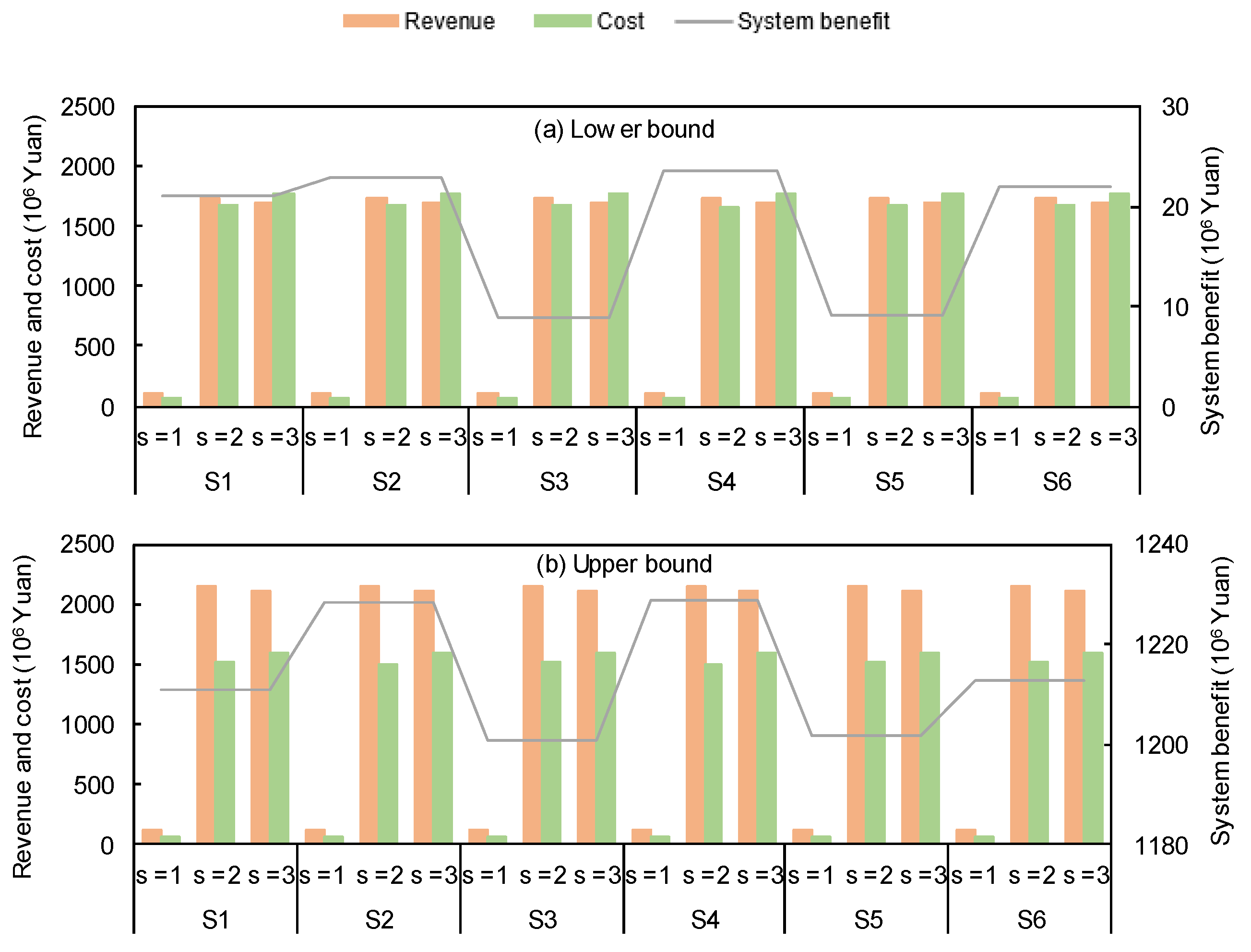
Figure 3 shows revenues and costs of each city as well as system benefit (i.e., f = total revenue minus total cost) under each scenario. Results show that the lowest f would be [8.9, 1200.6] × 10⁶ Yuan (under S3), and the highest f would be [23.6, 1228.8] × 10⁶ Yuan (under S4). The total revenue of the cities would be [3544.2, 4380.3] × 10⁶ Yuan under each scenario due to the unchanged cropland area targets. Different scenarios present different water availability levels and corresponding probabilities, leading to changed total costs. The lowest cost would be [3151.5, 3520.5] × 10⁶ Yuan (under S4), and the highest cost would be [3179.7, 3535.2] × 10⁶ Yuan (under S3). It is revealed that water resources availability can affect the economic development. Xiamen would contribute the lowest revenue and cost to the system economy. For instance, under S1, the revenue and cost of Xiamen would occupy 2.76% and [2.01, 2.09]% of the total amounts, respectively. Quanzhou would contribute the highest revenue and cost to the system economy. It is worth noting that the lower bound of cost would be higher than the lower bound of revenue, indicating high economic financial risk exists in the city. The difference would reach [71.95, 76.46] × 10⁶ Yuan (under S3).

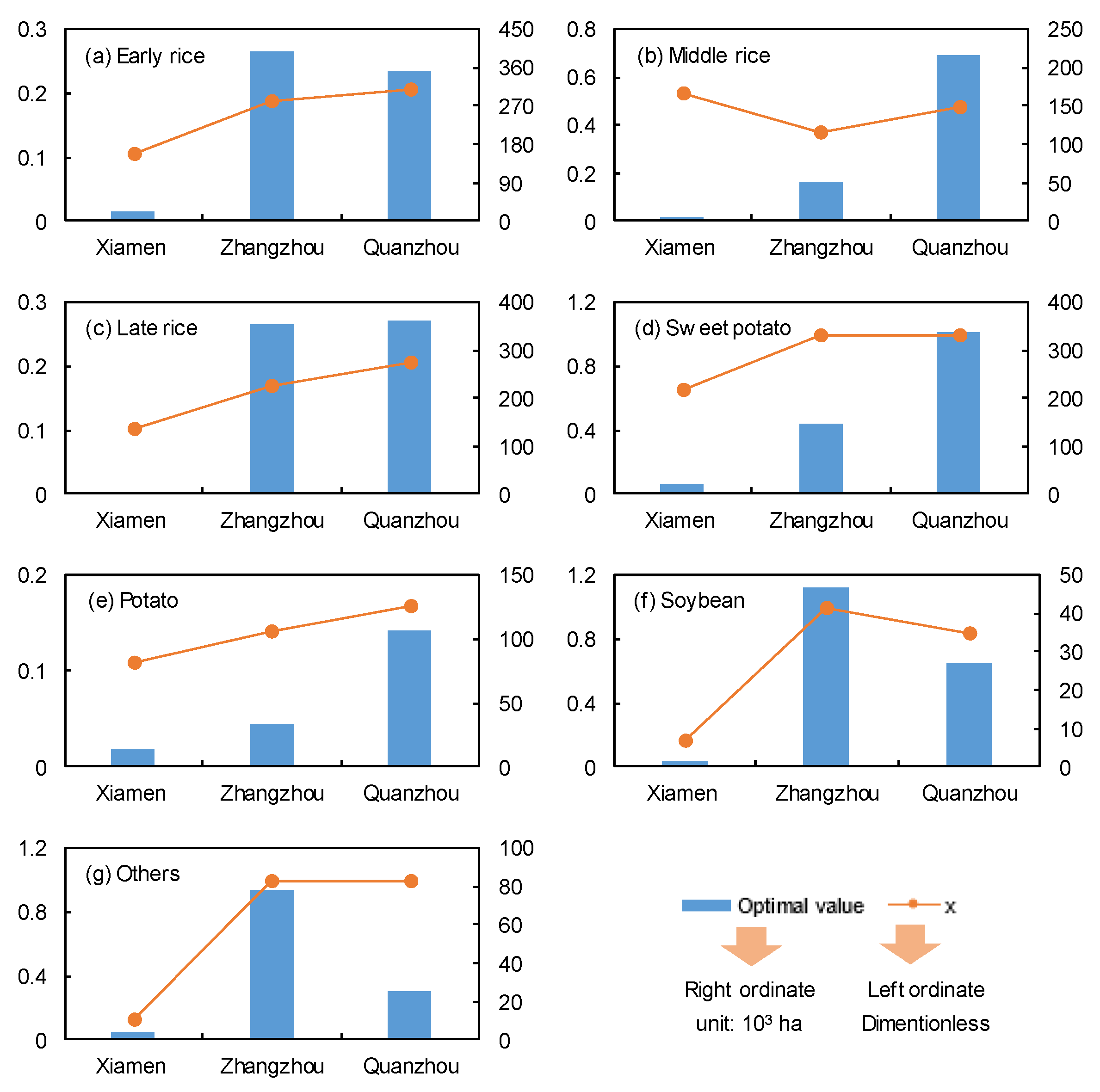
A cropland area target is pre-regulated for each crop in each city before the amounts of random available water resources are known. Figure 4 displays the optimal cropland area target. Total cropland area of the cities would be 2605.42 × 10³ ha (with Xiamen 2.7%, Zhangzhou 42.6%, and Quanzhou 54.7%). This may be attributed to the rapid urban construction of Xiamen, leading to the shrinking of cropland area. The development of Zhangzhou and Quanzhou still heavily rely on crop cultivation. The proportions of early rice and late rice would be 29.7% and 27.6%, respectively. This may be associated with climatic conditions, soil properties, market prices, and crop yields. Cropland area in sweet potato, soybean, and others in Quanzhou would be set as their upper bounds (i.e., x = 1), indicating decision makers take optimistic attitudes (due to high crop yields and market prices).

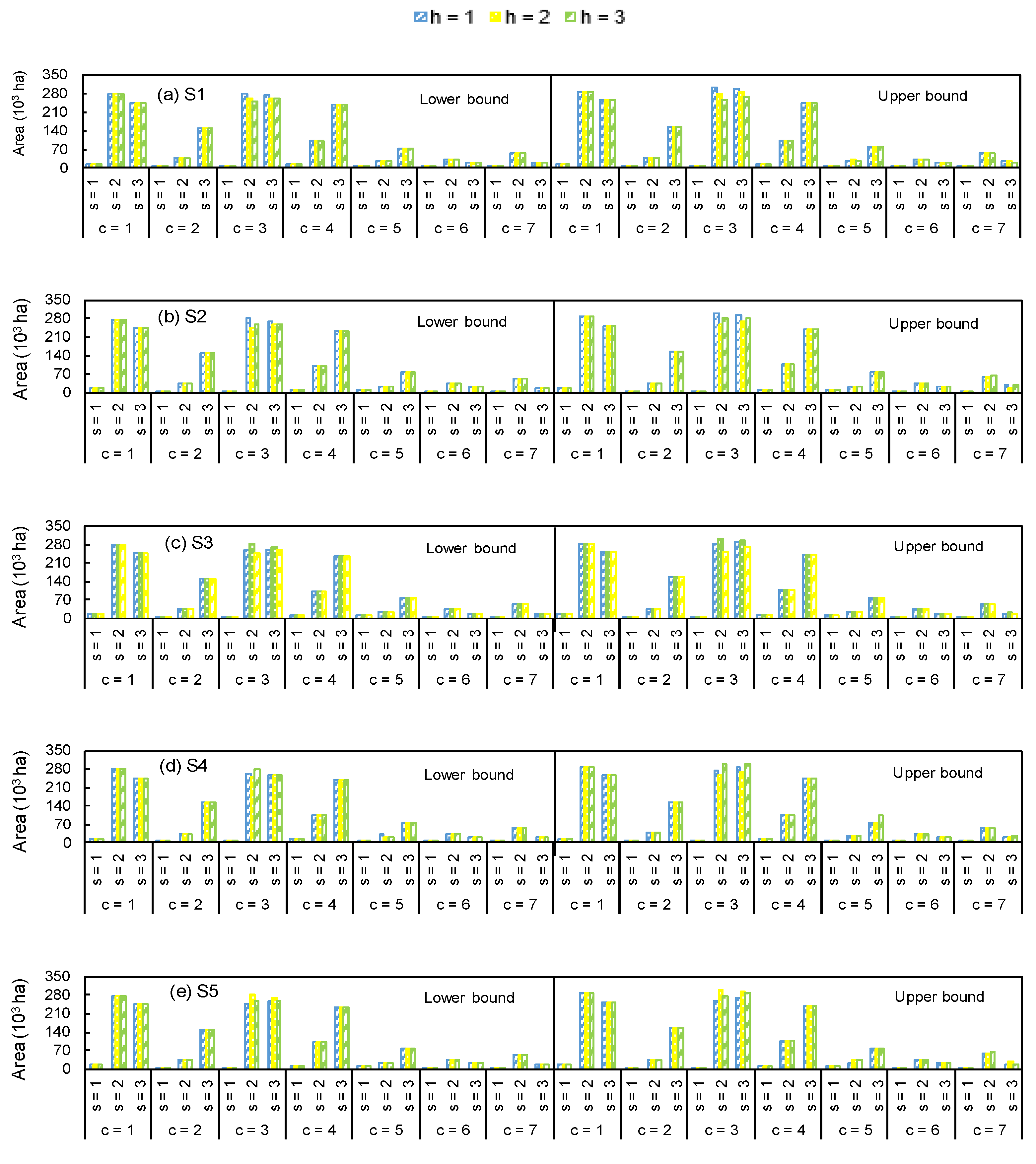
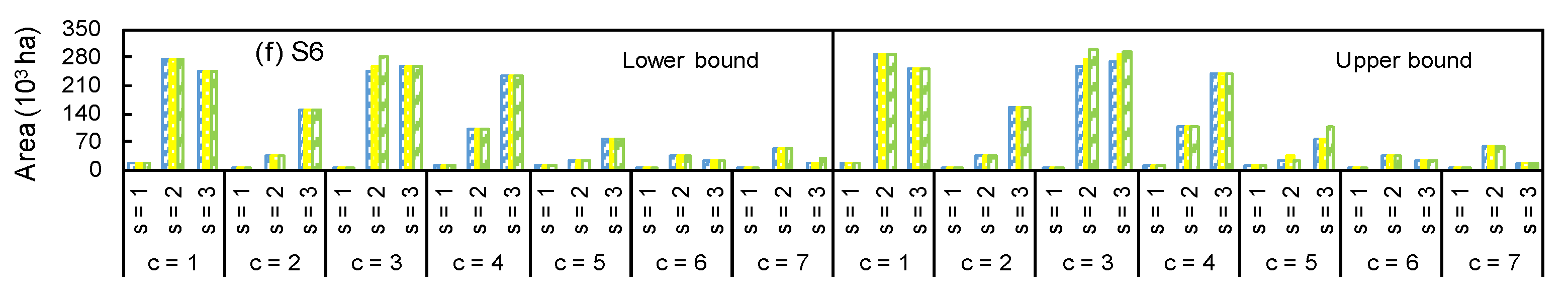
The targeted croplands are irrigated by surface water and groundwater. Figure 5 and Figure 6 summarize the optimal irrigation patterns of different crops under various available water scenarios. The proportion of cropland irrigated by surface water would be about [71.3, 73.8]%. This is mainly because of the high available surface water. Different scenarios would result in varied irrigation patterns. For instance, under S1, the area irrigated by surface water and groundwater would be [1877.8, 1967.2] × 10³ ha (low level) and [638.2, 727.6] × 10³ ha (low level); under S4, the area irrigated by surface water and groundwater would be [1852.6, 1926.6] × 10³ ha (low level) and [669.5, 762.1] × 10³ ha (medium level). It is found that Zhangzhou would be the most sensitive city to the changed available water resources (other cropland irrigation patterns would not change), due to relatively high cropland, limited water resources, and high demand of electricity for surface water. Under a certain scenario, irrigation patterns would also change with the varied available water level. For instance, under S6, the area irrigated by surface water would be [1831.0, 1885.6] × 10³ ha, [1843.3, 1935.9] × 10³ ha, and [1871.9, 1988.9] × 10³ ha under low, medium, and high levels, respectively. It is disclosed that surface water is more competitive than groundwater. This is associated with water price, irrigation quota, and available water.

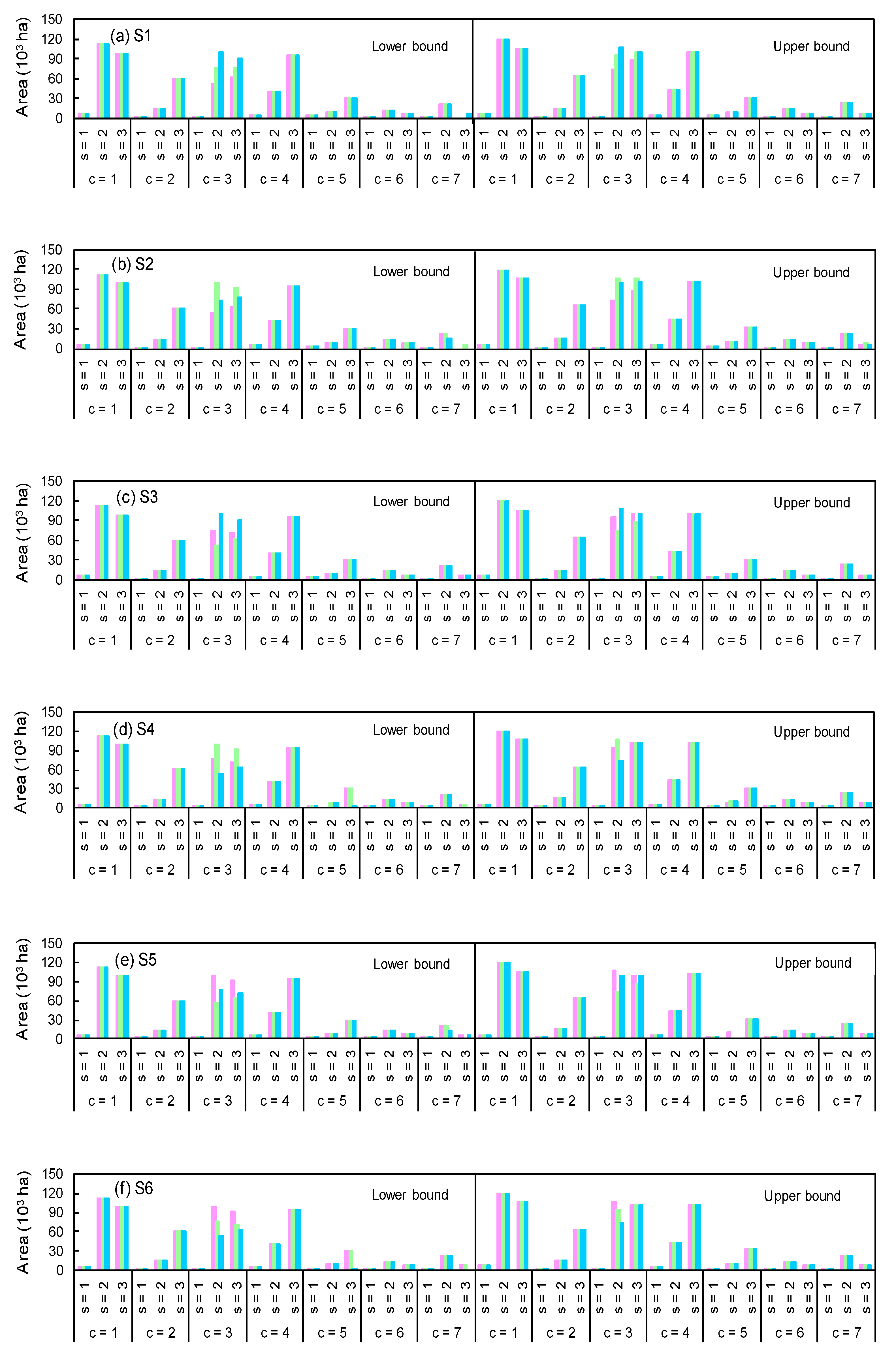
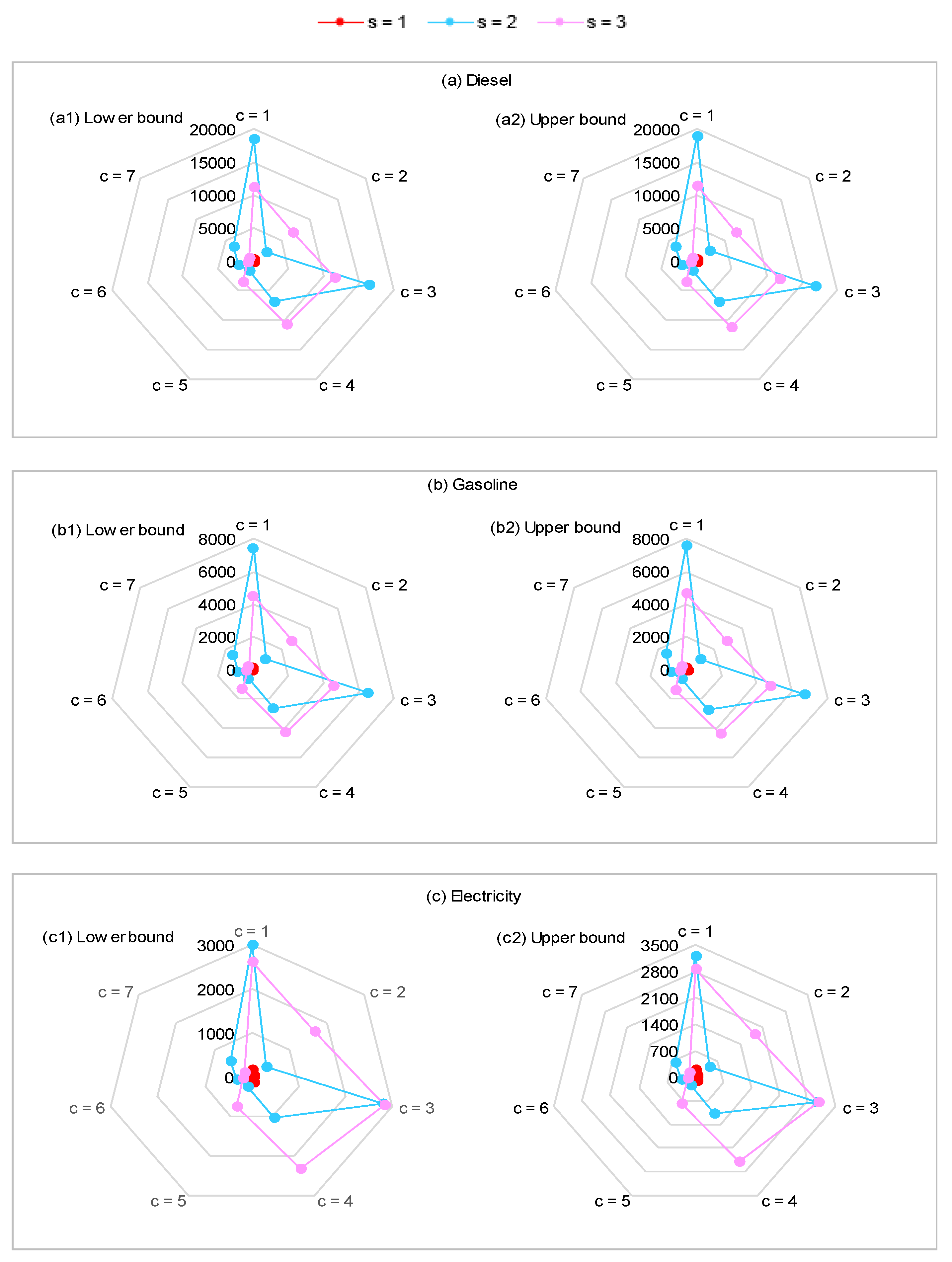
Figure 7 shows the optimal water allocation policy. It is found that surface water would take a high fraction of the total water supply (approximately [71.34, 73.68]%). Groundwater with higher water price and lower availability would be considered as a flexible supplementary resource to guarantee water safety for crop production under random available levels. Water allocated to early rice and late rice would, respectively, be [31.17, 31.53]% and [35.46, 36.12]% of the total water supply, due to their high cropland area targets and irrigation quota. Figure 8 lists the optimal energy consumption policy. Diesel agricultural machinery would share a large proportion of tillage, irrigation, drainage, and harvesting (serving for more than 60% of the total cropland area). The optimal energy consumption amount would be [97.4, 100.3] × 10³ L of diesel (liter), [38.9, 40.1] × 10³ L of gasoline, and [19.4, 20.9] × 10³ kWh of electricity (a proportion of [4.23, 5.01]% would contribute to water allocation). Zhangzhou would be the main energy consumer, which would consume [51.23, 52.12]% of the total energy.

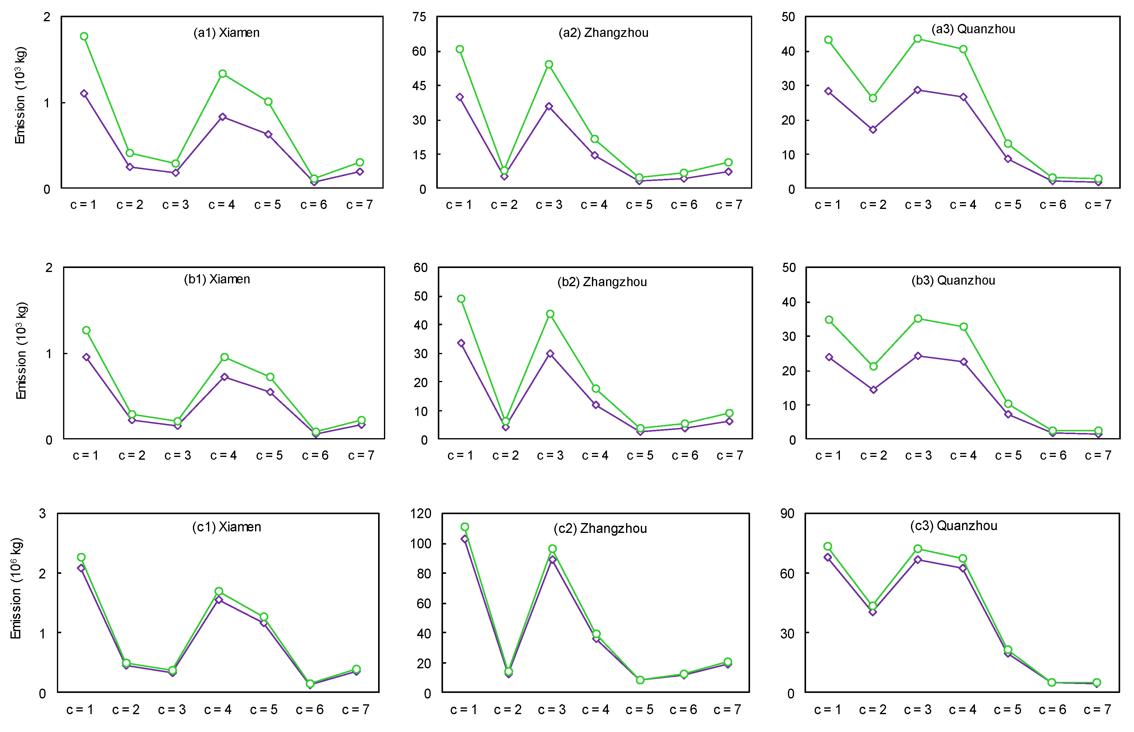
Figure 9 presents the embodied carbon and effluent emissions in per unit crop. The total amount of TN, TP, and CO₂ would be [226.9, 345.9] × 10³ kg, [190.7, 277.5] × 10³ kg, and [553.1, 598.7] × 10³ kg. Zhangzhou would contribute the highest emissions of TN and TP (occupying about 50.01% of the total emission), due to relatively high loss rate and unit fertilizer/pesticide application. The sources of carbon emission include diesel, gasoline, electricity, fertilizer, agricultural film, and pesticide. Quanzhou would contribute the highest emissions of CO₂ (occupying about 50.61% of the total emission), due to relatively high cropland area. In addition, decision makers should focus on early rice, late rice, and sweet potato. The emissions would account for more than 77.21% (TN), 77.45% (TP), 77.68% (CO₂) of the total emissions. This revealed a tradeoff between economic development and environmental protection.

4.2. Policy Security Assessment

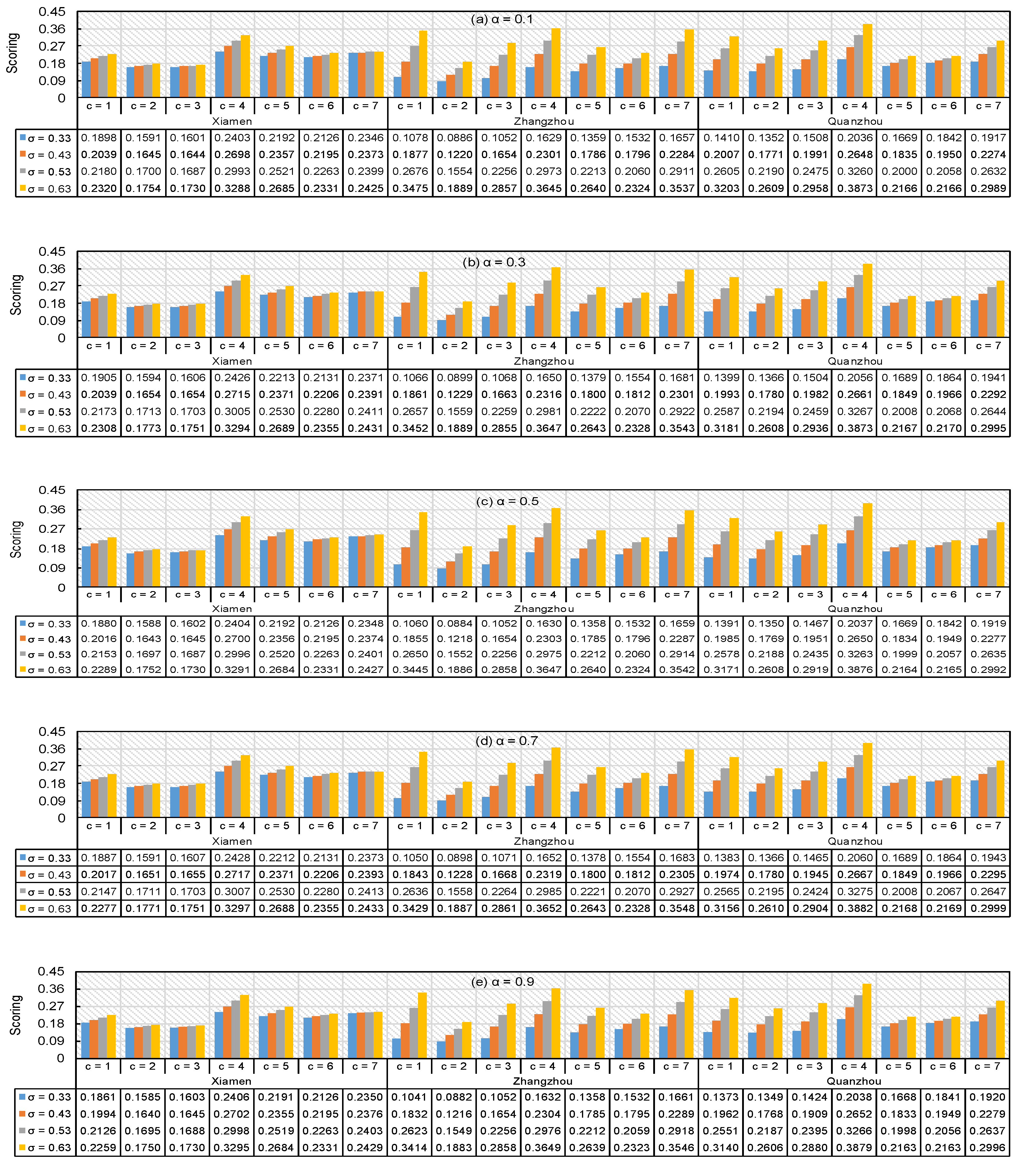
All new inputs of the IF-OWA method can then be calculated. As an example,

Table 6. New inputs of IF-OWA under α = 0.5.

Subarea	Criteria	Important Degree	Crop
			Early Rice	Middle Rice	Late Rice	Sweet Potato	Potato	Soybean	Others
Xiamen	CY	H	0.6002483	0.35282889	0.39235743	0.66759324	0.59732027	0	0.0102481
	CA	H	0.0474189	0.00834823	0.00498007	0.03523569	0.02593484	0	0.0055093
	MP	MH	0.0591787	0.01328502	0.01992754	0.36111111	0.01086957	0.2137681	0.7500000
	IQR	MH	0.1968750	0.04062500	0	0.6015625	0.59843750	0.7500000	0.3796875
	CAS	M	0.0273560	0.00481610	0.00287300	0.0203275	0.01496183	0	0.0031783
	CGS	M	0.4726438	0.49518368	0.49712678	0.47967229	0.48503796	0.4999998	0.4968214
	AD	LM	0.2440223	0.24999997	0.24497876	0.2423486	0.24545697	0.2425877	0.2418704
	AG	LM	0.2440223	0.24999997	0.24497876	0.2423486	0.24545697	0.2425877	0.2418704
	FA	L	0.1312614	0.13114817	0.13109155	0.1318277	0.13245059	0.1327337	0.1333000
	PU	L	0.0888667	0.11284656	0.11919418	0.12483651	0.11496243	0.1333333	0.1304788
Zhangzhou	CY	H	0.794963	0.7085858	0.6807694	0.8667000	0.7861789	0.2884120	0.8037471
	CA	H	0.8667000	0.1076609	0.7738350	0.3173617	0.0689270	0.0986499	0.1679816
	MP	MH	0.0525362	0.0048309	0.0108696	0.3544686	0.0018116	0.1926329	0.7167874
	IQR	MH	0.1968750	0.0406250	0	0.6015625	0.5984375	0.7500000	0.3796875
	CAS	M	0.4999999	0.0621096	0.4464260	0.1830862	0.0397640	0.0569112	0.0969087
	CGS	M	0	0.4378902	0.0535739	0.3169136	0.4602357	0.4430886	0.4030911
	AD	LM	0	0.0030655	0.0030655	0.0036785	0.0024524	0.0055178	0.0055178
	AG	LM	0	0.0030655	0.0030655	0.0036786	0.0024524	0.0055179	0.0055179
	FA	L	0	0.0005663	0.0005663	0.0084941	0.0118917	0.0141568	0.0203857
	PU	L	0	0.0832243	0.1029725	0.1170783	0.1121413	0.1255418	0.1262471
Quanzhou	CY	H	0.6163525	0.6983377	0.5782880	0.5036230	0.2386353	0.1434740	0.4889828
	CA	H	0.7690233	0.4682947	0.7858641	0.7347731	0.2310799	0.0556687	0.0518456
	MP	MH	0.0501208	0.0018116	0.0012077	0.3520531	0	0.1799517	0.7083333
	IQR	MH	0.1968750	0.0406250	0	0.6015625	0.5984375	0.7500000	0.3796875
	CAS	M	0.4436502	0.2701596	0.4684244	0.4238912	0.1333102	0.0321153	0.0299098
	CGS	M	0.0563497	0.2298403	0.0835024	0.0761087	0.3666896	0.4678845	0.4700900
	AD	LM	0.1006388	0.1006388	0.1006388	0.1006388	0.1006388	0.1006388	0.1006388
	AG	LM	0.1006389	0.1006389	0.1006389	0.1006389	0.1006389	0.1006389	0.1006389
	FA	L	0.0605909	0.062856	0.0634223	0.0645548	0.0645548	0.0673862	0.0679524
	PU	L	0.0056423	0.089572	0.1079095	0.1213101	0.1156677	0.1269524	0.1290683

displays new inputs under α = 0.5. Figure 10 shows the integrated scoring for the planning strategies of crops in the cities under different α and σ values. Under a certain α value, the scoring would increase with the raised σ values. For instance, when α = 0.1, the scoring of early rice in Xiamen would be 0.1898 (σ = 0.33), 0.2039 (σ = 0.43), 0.2180 (σ = 0.53), 0.2320 (σ = 0.63). High σ values represent high satisfaction of decision makers towards the system, leading to high scoring (i.e., high security). Under a certain σ value, the scoring would vary with the changed α value. For instance, when σ = 0.43, the scoring of each evaluation object would be 0.2039, 0.1645, 0.1644, 0.2698, 0.2357, 0.2195, 0.2373, 0.1877, 0.1220, 0.1654, 0.2301, 0.1786, 0.1796, 0.2284, 0.2007, 0.1771, 0.1991, 0.2648, 0.1835, 0.1950, and 0.2274 (ranking as 9, 19, 20, 1, 4, 8, 3, 13, 21, 18, 17, 16, 15, 6, 10, 17, 11, 2, 14, 12, and 7) under α = 0.1; the scoring of each evaluation object would be 0.1994, 0.1640, 0.1645, 0.2702, 0.2355, 0.2195, 0.2376, 0.1832, 0.1216, 0.1654, 0.2304, 0.1785, 0.1795, 0.2289, 0.1962, 0.1768, 0.1909, 0.2652, 0.1833, 0.1949, and 0.2279 (ranking as 9, 20, 19, 14, 8, 3, 14, 21, 18, 17, 16, 15, 6, 10, 17, 12, 2, 13, 11, and 7) under α = 0.9. Higher α values represent more progressive attitudes of decision makers (while higher risk levels of suffering system infeasibility), and thus more croplands, less investments, and less resources would be put to use in order to meet local demand.

In addition, under σ = 0.33, sweet potato, others, potato, and soybean of Xiamen are in the top four ranks; under σ = 0.43, sweet potato of Xiamen, sweet potato of Quanzhou, others of Xiamen, potato of Xiamen are in the top four ranks; under σ = 0.53, sweet potato of Quanzhou, sweet potato of Xiamen, sweet potato of Zhangzhou, others of Zhangzhou are in the top four ranks; under σ = 0.63, sweet potato of Quanzhou, sweet potato of Zhangzhou, others of Zhangzhou, early rice of Zhangzhou are in the top four ranks. Sweet potato and others would be the crops with the highest safety performance (especially sweet potato). This may be derived from their high market price, high crop yield, and low irrigation quota. Zhangzhou would be the city with highest comprehensive safety performance, due to the high revenue. The decision maker can select the final optimal alternative according to his/her risk tolerance.

5. Discussion

Th main findings can be summarized as follows: (a) the interactions between available surface water and groundwater can change the irrigation patterns and thus affect the system benefit. System benefit would increase by [2.34, 165.16]% from the lowest value to the highest value. (b) The shares of cropland area targets are 2.7% (Xiamen), 42.6% (Zhangzhou), and 54.7% (Quanzhou). (c) Early rice and late rice are main water consumers (occupying [31.17, 31.53]% and [35.46, 36.12]% of the total water supply). (d) More than 60% of the total cropland area were served by diesel agricultural machinery. (e) Zhangzhou is the most sensitive city to the changed available water resources. (f) Zhangzhou contributes 50.01% of the total TN and TP emissions, while Quanzhou contributes 50.61% of the total CO₂ emission. (g) Security level of cities and crops change with the varied σ and α values. Decision makers may need to (i) prepare emergency plans in case of low available water resources. (ii) Ensure sufficient water supply to early rice and late rice. (iii) Enhancement policies such as changing topographic slope, improving soil quality, promoting cropland drainage, and using energy-mix machine should be conducted. (iv) Pay attention to the development in the Zhangzhou city. (v) Conduct security assessment before making decisions.

The developed ISF-PA model can be applied to coordinate food production, water resource allocation, and energy consumption in a sustainable manner. A shortcoming of the model is that it can only account for the expected second-stage cost without any consideration on the variability of the cost under a certain available water level, such that Quanzhou suffers economic deficits. This may be unacceptable for local policy makers. Financial risk management methods are attractive techniques that could help tackle the above shortcoming, which is launched to control the variability of the recourse cost, as well as to capture the notion of risk. The impacts of other environmental policies such as carbon mitigation, air pollution control, water pollutant should also gain more concern. This is the first attempt to apply the developed model in the study area. It was difficult to compare current results with the other authors. In future works, comparison is needed since it can highlight the innovations of the current research.

6. Conclusions

In this study, an interval-stochastic-fuzzy policy analysis (ISF-PA) model was proposed to generate optimal security management policy for a water–energy–food nexus system. The model was applied to a practical study of a comprehensive issue in the Xiamen-Zhangzhou-Quanzhou urban agglomeration, Fujian province, China. In the application, surface water and groundwater availability were expressed as probability distributions; linguistic quantifiers were presented as triangular fuzzy membership functions; others were shown as interval values. The developed model provides the optimal policies of cropland planning, water allocation, energy consumption, as well as carbon and effluent emissions; meanwhile, the system security of different crops in different cities were evaluated.

References

- Namany, S.; Al-Ansari, T.; Govindan, R. Sustainable energy, water and food nexus systems: A focused review of decision-making tools for efficient resource management and governance. J. Clean Prod. 2019, 225, 610–626. [Google Scholar] [CrossRef]
- Elagib, N.A.; Al-Saidi, M. Balancing the benefits from the water–energy–land–food nexus through agroforestry in the Sahel. Sci. Total Environ. 2020, 742, 140509. [Google Scholar] [CrossRef] [PubMed]
- Zhang, S.; Rasool, G.; Guo, X.; Sen, L.; Cao, K. Effects of different irrigation methods on environmental factors, rice production, and water use efficiency. Water 2020, 12, 2239. [Google Scholar] [CrossRef]
- Baradei, S.E.; Sadeq, M.A. Effect of solar canals on evaporation, water quality, and power production: An optimization study. Water 2020, 12, 2103. [Google Scholar] [CrossRef]
- Al-Saidi, M.; Elagib, N.A. Increasing resource interlinks due to growing scarcities, resources supply crises and failures of sector-driven management strategies justified the need for the cross-sectoral integration of the resources. Sci. Total Environ. 2017, 574, 1131–1139. [Google Scholar] [CrossRef]
- Bréthaut, G.; Gallagher, L.; Dalton, J.; Allouche, J. Power dynamics and integration in the water-energy-food nexus: Learning lessons for transdisciplinary research in Cambodia. Environ. Sci. Policy 2019, 94, 153–162. [Google Scholar] [CrossRef] [Green Version]
- Zhang, P.P.; Zhang, L.X.; Chang, Y.; Xu, M.; Hao, Y.; Liang, S.; Liu, G.Y.; Yang, Z.F.; Wang, C. Food-energy-water (FEW) nexus for urban sustainability: A comprehensive review. Resour. Conserv. Recycl. 2019, 142, 215–224. [Google Scholar] [CrossRef]
- Mitschele-Thiel, A. Integrating model-based optimization and program transformation to generate ecient parallel programs. J. Sys. Architect. 1999, 45, 465–482. [Google Scholar] [CrossRef]
- Leung, P.H.; Martinez-Hernandez, E.; Leach, M.; Yang, A.D. Designing integrated local production systems: A study on the food-energy-water nexus. J. Clean Prod. 2016, 135, 1065–1084. [Google Scholar] [CrossRef]
- Si, Y.; Li, X.; Yin, D.Q.; Li, T.J.; Cai, X.M.; Wei, J.H.; Wang, G.Q. Revealing the water-energy-food nexus in the Upper Yellow River Basin through multi-objective optimization for reservoir system. Sci. Total Environ. 2019, 682, 1–18. [Google Scholar] [CrossRef]
- Sadeghi, S.H.; Moghadam, E.S.; Delavar, M.; Zarghami, M. Application of water-energy-food nexus approach for designating optimal agricultural management pattern at a watershed scale. Agric. Water Manag. 2020, 233, 106071. [Google Scholar] [CrossRef]
- Guan, X.; Mascaro, G.; Sampson, D.; Maciejewski, R. A metropolitan scale water management analysis of the food-energy-water nexus. Sci. Total Environ. 2020, 701, 134478. [Google Scholar] [CrossRef] [PubMed]
- Wu, L.N.; Elshorbagy, A.; Pande, S.; Zhuo, N. Trade-offs and synergies in the water-energy-food nexus: The case of Saskatchewan, Canada. Resour. Conserv. Recycl. 2021, 164, 105192. [Google Scholar] [CrossRef]
- Núñez-López, J.M.; Rubio-Castro, E.; Ponce-Ortega, J.M. Involving resilience in optimizing the water-energy-food nexus at macroscopic level. Process Saf. Environ. 2021, 147, 259–273. [Google Scholar] [CrossRef]
- Chamas, Z.; Najm, M.A.; Al-Hindi, M.; Yassine, A.; Khattar, R. Sustainable resource optimization under water-energy-food-carbon nexus. J. Clean Prod. 2021, 278, 123894. [Google Scholar] [CrossRef]
- Wang, J.J.; Jing, Y.Y.; Zhang, C.F.; Zhao, J.H. Review on multi-criteria decision analysis aid in sustainable energy decision-making. Renew. Sustain. Energy Rev. 2009, 13, 2263–2278. [Google Scholar] [CrossRef]
- Khan, I. Power generation expansion plan and sustainability in a developing country: A multi-criteria decision analysis. J. Clean. Prod. 2019, 220, 707–720. [Google Scholar] [CrossRef]
- Butchart-Kuhlmann, D.; Kralisch, S.; Fleischer, M.; Meinhardt, M.; Brenning, A. Multicriteria decision analysis framework for hydrological decision support using environmental flow components. Ecol. Indic. 2018, 93, 470–480. [Google Scholar] [CrossRef]
- Wang, L.; Ma, G.Y.; Zhou, F.; Li, Y.; Tian, T. Multicriteria decision-making approach for selecting ventilation heat recovery devices based on the attributes of buildings and the preferences of decision makers. Sustain. Cities Soc. 2019, 51, 101753. [Google Scholar] [CrossRef]
- Zhu, F.L.; Zhong, P.; Cao, Q.; Chen, J.; Sun, Y.M.; Fu, J.S. A stochastic multi-criteria decision making framework for robust water resources management under uncertainty. J. Hydrol. 2019, 576, 287–298. [Google Scholar] [CrossRef]
- Balezentis, T.; Chen, X.L.; Galnaityte, A.; Namiotko, V. Optimizing crop mix with respect to economic and environmental constraints: An integrated MCDM approach. Sci. Total Environ. 2020, 705, 135896. [Google Scholar] [CrossRef] [PubMed]
- Paul, M.; Negahban-Azar, M.; Shirmohammadi, A.; Montas, A. Assessment of agricultural land suitability for irrigation with reclaimed water using geospatial multi-criteria decision analysis. Agric. Water Manag. 2020, 231, 105987. [Google Scholar] [CrossRef]
- Rubio-Aliaga, A.; García-Cascales, M.S.; Sánchez-Lozano, J.M.; Molina-Garci, A. MCDM-based multidimensional approach for selection of optimal groundwater pumping systems: Design and case example. Renew. Energy 2021, 163, 213–224. [Google Scholar] [CrossRef]
- Arjomandi, A.; Mortazavi, S.A.; Khalilian, S.; Garizi, A.Z. Optimal land-use allocation using MCDM and SWAT for the Hablehroud Watershed, Iran. Land Use Policy 2021, 100, 104930. [Google Scholar] [CrossRef]
- Zeng, X.T.; Zhang, J.L.; Yu, L.; Zhu, J.X.; Li, Z.; Tang, L. A sustainable water-food-energy plan to confront climatic and socioeconomic changes using simulation-optimization approach. Appl. Energy 2019, 36, 743–759. [Google Scholar] [CrossRef]
- Simic, V. A two-stage interval-stochastic programming model for planning end-of-life vehicles allocation under uncertainty. Resour. Conserv. Recycl. 2015, 98, 19–29. [Google Scholar] [CrossRef]
- Wang, Y.Z.; Li, Z.; Guo, S.S.; Zhang, F.; Guo, P. A risk-based fuzzy boundary interval two-stage stochastic water resources management programming approach under uncertainty. J. Hydrol. 2020, 582, 124553. [Google Scholar] [CrossRef]
- Guo, S.S.; Zhang, F.; Zhang, C.L.; Wang, Y.Z.; Guo, P. An improved intuitionistic fuzzy interval two-stage stochastic programming for resources planning management integrating recourse penalty from resources scarcity and surplus. J. Clean. Prod. 2019, 234, 185–199. [Google Scholar] [CrossRef]
- Kaya, İ.; Çolak, M.; Terzi, F. A comprehensive review of fuzzy multi criteria decision making methodologies for energy policy making. Energy Strateg. Rev. 2019, 24, 207–228. [Google Scholar] [CrossRef]
- Li, Y.P.; Huang, G.H.; Cui, L.; Liu, J. Mathematical modeling for identifying cost-effective policy of municipal solid waste management under uncertainty. J. Environ. Inform. 2019, 34, 55–67. [Google Scholar] [CrossRef] [Green Version]
- Mansouri, S.A.; Ahmarinejad, A.; Javadi, M.S.; Catalão, J.P.S. Two-stage stochastic framework for energy hubs planning considering demand response programs. Energy 2020, 206, 118124. [Google Scholar] [CrossRef]
- Hassanpour, A.; Roghanian, E. A two-stage stochastic programming approach for non-cooperative generation maintenance scheduling model design. Int. J. Electr. Power Energy Syst. 2021, 126, 106584. [Google Scholar] [CrossRef]
- Li, M.; Fu, Q.; Singh, V.P.; Liu, D.; Li, T.X. Stochastic multi-objective modeling for optimization of water-food-energy nexus of irrigated agriculture. Adv. Water Resour. 2019, 127, 209–224. [Google Scholar] [CrossRef]
- Huang, G.H.; Loucks, D.P. An inexact two-stage stochastic programming model for water resources management under uncertainty. Civ. Eng. Environ. Syst. 2000, 17, 95–118. [Google Scholar] [CrossRef]
- Kaur, G.; Dhar, J.; Guha, R.K. Minimal variability OWA operator combining ANFIS and fuzzy c-means for forecasting BSE index. Math. Comput. Simul. 2016, 122, 69–80. [Google Scholar] [CrossRef]
- Chen, Z.S.; Yu, C.; Chin, K.S.; Martínez, L. An enhanced ordered weighted averaging operators generation algorithm with applications for multicriteria decision making. Appl. Math. Model 2019, 71, 467–490. [Google Scholar] [CrossRef]
- Wang, X.; Kerre, E.E. Reasonable properties for the ordering of fuzzy quantities (I & II). Fuzzy. Sets Syst. 2001, 118, 375–405. [Google Scholar]
- Suo, M.Q.; Li, Y.P.; Huang, G.H. Multicriteria decision making under uncertainty: An advanced ordered weighted averaging operator for planning electric power systems. Eng. Appl. Artif. Intel. 2002, 25, 72–81. [Google Scholar] [CrossRef]
- Yager, R.R. On ordered weighted averaging aggregation operators in multicriteria decision making. IEEE Trans. Syst. Man Cybern. 1998, 18, 183–190. [Google Scholar] [CrossRef]
- XSY, Xiamen Statistical Yearbook; Xiamen Municipal Bureau of Statistics: Xiamen, China, 2019.
- ZSY, Zhangzhou Statistical Yearbook; Zhangzhou Municipal Bureau of Statistics: Zhangzhou, China, 2019.
- QSY, Quanzhou Statistical Yearbook; Quanzhou Municipal Bureau of Statistics: Quanzhou, China, 2019.
- FSY, Fujian Statistical Yearbook; Fujian Provincial Statistics Bureau: Fuzhou, China, 2019.
- CESY, China Energy Statistical Yearbook; National Energy Administration: Beijing, China, 2018.
- Li, M.; Fu, Q.; Singh, V.P.; Ji, Y.; Liu, D.; Zhang, C.; Li, T. An optimal modelling approach for managing agricultural water-energy-food nexus under uncertainty. Sci. Total Environ. 2019, 651, 1416–1434. [Google Scholar] [CrossRef]
- Yu, L.; Xiao, Y.; Zeng, X.T.; Li, Y.P.; Fan, Y.R. Planning water-energy-food nexus system management under multi-level and uncertainty. J. Clean. Pro. 2020, 251, 119658. [Google Scholar] [CrossRef]
- da Silva, L.P.B.; Hussein, H. Production of scale in regional hydropolitics: An analysis of La Plata River Basin and the Guarani Aquifer System in South America. Geoforum 2019, 99, 42–53. [Google Scholar] [CrossRef]
- Odeh, T.; Mohammad, A.H.; Hussein, H.; Ismail, M.; Almomani, T. Over-pumping of groundwater in Irbid governorate, northern Jordan: A conceptual model to analyze the effects of urbanization and agricultural activities on groundwater levels and salinity. Environ. Earth Sci. 2019, 78, 40. [Google Scholar] [CrossRef] [Green Version]
Figure 1.
The study area.
Figure 2.
Framework of the interval-stochastic-fuzzy policy analysis (ISF-PA) model.
Figure 3.
Revenues, costs, and benefits: (a) Lower bound, (b) Upper bound.
Figure 4.
Optimal cropland area target: (a) Early rice, (b) Middle rice, (c) Late rice, (d) Sweet potato, (e) Potato, (f) Soybean, (g) Others.
Figure 5.
Cropland irrigated by surface water: (a) S1, (b) S2, (c) S3, (d) S4, (e) S5, (f) S6.
Figure 6.
Cropland irrigated by groundwater: (a) S1, (b) S2, (c) S3, (d) S4, (e) S5, (f) S6.
Figure 7.
Water resources allocation: (a) Lower bound, (b) Upper bound.
Figure 8.
Energy consumption: (a) Diesel, (b) Gasoline, (c) Electricity.
Figure 9.
Carbon and effluent emissions: (a1) TN emission in Xiamen, (a2) TN emission in Zhangzhou, (a3) TN emission in Quanzhou, (b1) TP emission in Xiamen, (b2) TP emission in Zhangzhou, (b3) TP emission in Quanzhou, (c1) CO2 emission in Xiamen, (c2) CO2 emission in Zhangzhou, (c3) CO2 emission in Quanzhou.
Figure 10.
Integrated scoring for the planning policy: (a) α = 0.1, (b) α = 0.3, (c) α = 0.5, (d) α = 0.7, (e) α = 0.9.