The Impacts of Climate Change on Wastewater Treatment Costs: Evidence from the Wastewater Sector in China


1
School of Public Policy, University of California, Riverside, 900 University Ave., Riverside, CA 92521, USA
2
Environmental Economics and Natural Resources Group, Wageningen University & Research, P.O. Box 9101, 6700 HB Wageningen, The Netherlands
*
Author to whom correspondence should be addressed.
Water 2020, 12(11), 3272; https://doi.org/10.3390/w12113272
Submission received: 27 October 2020
/
Revised: 16 November 2020
/
Accepted: 19 November 2020
/
Published: 21 November 2020
(This article belongs to the Special Issue Water Management: New Paradigms for Water Treatment and Reuse)
Abstract
:Treatment of wastewater is expected to become a major development issue in the years to come. We investigate the relationship between climate and costs of wastewater treatment with the objective of examining if changes in climate might have an impact on the costs of wastewater treatment. For that purpose, we use a cross-section sample of 163 treatment plants from China to estimate the industry’s cost function. The methodology used comprises an econometric estimation procedure of treatment costs of the wastewater sector, and a simulation of changes in these costs predicted with future climate conditions, policy implementation scenarios, population growth and development trends. Our results find evidence of climate change impact on treatment costs. We also simulate potential impact of future policy and climate scenarios on costs of treatment, and we measure the cost impact of all other cost determinants but climate—as these are indirectly affected by accounting for climate in the estimation procedure. This indirect impact predicts total cost changes of different magnitudes across the range of future scenarios investigated.
1. Introduction
Economic development, urbanization, and population growth trends are raising the demand for water around the world. The uncertainty of future conditions, most noticeably climate change, urges society to decide upon and pay in advance for mitigation efforts. This, in turn, requires quantification of the distribution of outcomes following both action and inaction strategies. One such strategy could be the reuse of treated wastewater for beneficial purposes, a phenomenon which unsurprisingly is currently gaining traction mainly in arid and semi-arid regions in the world [1].
Reuse of treated wastewater can mitigate water scarcity. As a relatively stable source of supply it can substitute for natural fresh water sources. However, the costs of the treatment process, those associated with direct input use, and those potentially affected by regulatory requirements, quality enhancement considerations and others, might hinge on the attractiveness of this solution. Surprisingly, wastewater treatment, which is also an activity of a public good nature, was studied thus far mostly among engineers and at the outskirts of economic research. Our objective in this paper is therefore to enrich the literature by examining if changes in climate might have an impact on the costs of wastewater treatment. This will be, to the best of our knowledge the first contribution to do so. If indeed costs of treatment are impacted by climate changes, any analysis ignoring them is either over, or underestimating the desirability of wastewater reuse to society.
A recent survey [1] identified the untapped potential of wastewater reuse in the world. Of the 181 countries surveyed in the period between 1995 to 2012, 40 and 30 percent provided partial and complete information, respectively, on wastewater generated, treated, and reused, reported in cubic kilometers per year. While not a complete count, this data set suggests that global wastewater generated, treated, and reused annually amounts to 340, 165, and 24 km3, respectively. This is a significant potential that has not yet been tapped sufficiently in many countries. Using Israel as a case study, [2] valued the contribution of treated wastewater reuse to the local water economy on a long-term planning horizon by approximately 330 to 460 thousand USD per 1 million m3 of reused water annually, depending on the level of natural recharge assumed. While these estimates are obviously dependent on local conditions, which most likely vary considerably on a global scale, the figures cited above yield an estimate of some 46 to 64 billion USD in worldwide economic welfare that could be realized annually through reuse of existing treated wastewater. An alternative measure is an equivalent of about 54 to 76 percent of the estimated value of future damages to water resources associated with a 1 C° increase in global mean temperature [3]. Thus, the potential of returning these benefits to the economy cannot be ignored. Furthermore, if indeed the objective of cutting untreated wastewater disposal globally in half by 2030 will materialize, as indicated in SDG 6.3 and SDG 6.3.1 of the Sustainable Development Goals report [4], these benefits can even be larger.
As more countries realize the role of wastewater in their water resources management, and invest public and private funds in wastewater systems, several points of caution must be addressed. The multiple effects of population increase and climate change impacts on water resources and water services have ramifications for policy, which is the aim of this paper.
The paper develops as follows: Next we review the literature concerned with the likely impacts of climate change on the water and wastewater sectors, and why they are critical for policy. In Section 3 we describe the situation in China that is used to apply our approach; we also present in detail the dataset used for the estimation of the cost function. Section 4 describes the methodological components of empirical framework and specifications, and derived simulations. In Section 5, we present the results of the econometric estimation of a sector-level treatment cost function. Section 6 presents simulations of future climate change scenarios and their impact on wastewater treatment costs, using the estimated cost function parameters from Section 5. Section 7 concludes and addresses policy implications of our analysis and results.
2. Literature Review
Scientists’ predictions of climate change impacts on various sectors have already materialized in many parts of the world [5,6,7]. Sectors that are most vulnerable to climate change include agriculture and water resources. Some of the impacts of climate change that are predicted to affect these sectors include temperature increase and alteration of precipitation patterns [8]. For the most part, economic literature on the impacts of climate change addressed its effects on agricultural productivity, using both econometric and programming approaches (an appropriate coverage of both can be found in [9,10,11,12], and references therein). A prominent discussion within the associated econometric literature is concerned with the usefulness of different methods to identify the true impact of climate change in order to elicit relevant policy actions [9,13,14]. Contributing to this discussion, Reference [11] (page 107) summarized the debate and highlighted the essence of the different arguments by stating that:
“Due to omitted variables concerns in the cross-sectional approach the recent literature has preferred the latter panel approach, noting that while average climate could be correlated with other time-invariant factors unobserved to the econometrician, short-run variation in climate within a given area (typically termed “weather”) is plausibly random and thus better identifies the effect of changes in climate variables on economic outcomes.While using variation in weather helps to solve identification problems, it perhaps more poorly approximates the ideal climate change experiment. In particular, if agents can adjust in the long run in ways that are unavailable to them in the short run, then impact estimates derived from shorter run responses to weather might overstate damages from longer run changes in climate.”
It has been noted that climate change could also significantly affect the human-built infrastructure through increasing uncertainty in future air temperature, precipitation, wind speed, and rise in sea level. Climate change may thus influence existing and planned urban water systems [15,16]. The wastewater sector is being affected by climate change in various ways. For example, higher amounts of pathogens could be carried to the wastewater treatment plant (WWTP) if it is connected to storm water collection systems. Higher levels of rainfall also can increase flows of sewage fed via the collection system. These two types of events can lead to operational needs beyond the treatment plant’s capacity, thus, impacting reliability and operating costs [17,18,19]. Another impact of climate change on wastewater treatment performance is its effects on the biological processes used in treatment plants, specifically dropping the nitrogen removal rate [20,21,22]. In particular, Reference [22] (page 202) found that intra-annual variations in temperature affect the performance of anaerobic reactors and stabilization ponds, compared with activated sludge, and aerobic biofilm reactors that are less sensitive to temperature fluctuations due to their “higher technological input and mechanization levels.” [23] also identify potential challenges in the operation of a wastewater treatment plant resulting from changes in temperatures. The authors emphasize the sensitivity of the treatment process to temperature extremes. Because WWTPs are designed for a range of assumed flows and sewage characteristics, as well as climatic conditions, any changes to the designed values may lead to under performance or even failure [20].
Referring to the earlier discussion regarding climate change impacts on agricultural productivity and the adaptation measures that can potentially be feasible under this setting, it is important to note that the impacts on the wastewater sector we just reviewed are much more mechanical in nature than the effects on food production. Therefore, contrary to the agricultural sector, the set of tools existing at the individual decision unit level (i.e., treatment plant versus a farm) are much more limited. Generally, even at a higher decision-making level, the notion of adaptation seems to be a very complex task in the wastewater treatment sector [23]. It is, therefore, quite surprising that despite the engineering observations regarding impact of climate change on wastewater treatment performance, most of the recent economic estimates of wastewater treatment cost functions that we are aware of (e.g., [24,25,26,27,28]) do not account for any future climate impacts.
3. Wastewater Treatment in China and Data
China was selected as the focus of our approach in this study for various reasons. First, data on economic variables of a major component of the wastewater industry is readily available. Second, China is a growing economy with major investments in the wastewater sector. Third, China faces climate variation across the landscape of the wastewater treatment facilities around the country. Finally, increased attention is given to climate impacts on the wastewater treatment sector in China, due to the large amount of energy and chemicals consumed in wastewater treatment processes [29,30], and because government regulations of urban drainage and sewage treatment require that climate trajectories should be considered in the process of wastewater treatment planning [31].
3.1. The Wastewater Sector of China
With fast industrialization and urban growth, wastewater discharge in China has increased from 48.2 billion tons (~m3) in 2004, to 71.1 billion tons (~m3) in 2016 [32]. Construction of WWTPs has also intensified over this period. Between 2006 and 2016, the number of WWTPs has more than tripled, increasing from 1019 to 3552, with treatment capacity increasing from 68.62 to 179.46 million m3 per day [33] (several official data sources demonstrate variation in total number of treatment plants reported in the industry. After consulting with a professional in this field, we decided to use the current reference. While these differences amount to roughly 20 percent, we do not think they should significantly affect the analyses presented in the paper). This development is, however, unbalanced geographically and across urban and rural centers [34].
The treatment technologies mostly used in China are conventional Activated Sludge process (AS), Oxidation Ditch, Sequencing Batch Reactors (SBR), Anaerobic/Anoxic/Oxic (AAO), and Anoxic-Oxic (AO) processes. Less widely used are Biofilm processes, Membrane Bioreactors (MBR), natural biologic treatment systems (e.g., constructed wetland), and Anaerobic Biologic treatment processes [35,36]. Nearly 75 percent of WWTPs in China are medium-size (1–10 × 104 m3/day). Small (<1 × 10⁴ m3/day) and medium WWTPs mainly use Oxidation Ditch and SBR processes, while the majority of large plants (>10 × 104 m3/day) use AAO processes [35].
The WWTPs in China follow the national standards determining the quality of treated wastewater discharge (defined under regulation titled GB 18918–2002). This standard defines four classes for effluent disposal, separated by the levels of constituents imposed under each class [37]. These classes are determined based on the age of the treatment plant as well as on the receiving water body [30]. The wastewater effluent meeting Class 1A can be reused or discharged to a recreational or scenic water body. Class 1B effluents can be reused or disposed of to the sea through running rivers or streams [38]. In addition to the national standard, every province may issue its own effluent discharge standard, and the local standard must be stricter than or equal to the national standard. According to [35] only 20 out of 31 provinces in mainland China have issued such standards.
3.2. Description of the Data
We analyze a cross-section data of 163 WWTPs from China, sampled in 2006. The dataset is described in detail in [28], and [39]. Due to data misspecification regarding the year of establishment, we had to remove two plants from the original sample. For each WWTP in the dataset, we obtained its geo-reference, the year of establishment and associated investment, its treatment capacity, the actual volume treated in 2006, several quality parameters of influent and effluent water, and the annual operating and maintenance (O&M) costs. The descriptive statistics of these variables is presented in Table 1.
We also use information regarding the treatment processes (technologies) used in each plant. Following [36], these are divided into eight groups as depicted in Table 2 (We refer the interested reader to [40] for detailed information regarding the characteristics of the different processes). We also report in Table 2 the share of each technology group in the WWTPs and in the total designed capacity in our sample. We compare these shares to those reported by [35], based on data from 2012, and by [36], based on data from 2013, for the entire wastewater treatment sector in China (these two sources present slight to moderate differences in reporting, and both rely on official and reliable data sources).
It appears from Table 2 that AAO technology is underrepresented in our sample, and that Oxidation Ditch and AS technologies are overrepresented, compared to the data reported in the other two sources. The rest of the sample seem to be representative of the entire population in terms of technologies used. As reported earlier, China’s wastewater treatment industry had developed dramatically between 2006, the year of our sample, and the years reviewed by [35,36]. It seems natural that some of the differences appearing in Table 2 might be a result of that rapid development. Nevertheless, we calculate sampling weights based on these differences and introduce them into the estimation procedure, which is described in the following sections.
To include the impact of climate on the cost of wastewater treatment, we supplemented the dataset with long-term weather data taken from the widely used Climatic Research Unit (CRU) database [41]. We used the inverse distance weighting (IDW) method in order to fit each WWTP in the sample with its own set of climate variables. For each treatment plant in the sample, we computed both historical and the sample period values of each climate indicator as depicted in Table 3, i.e., based on the year of establishment, we computed for each plant its unique 30-year historical average of each climate variable listed in Table 3. We also computed for each plant the same variable (observed weather) for the year 2006, the year of our sample. Descriptive statistics summary of these climate variables is presented in Table 3.
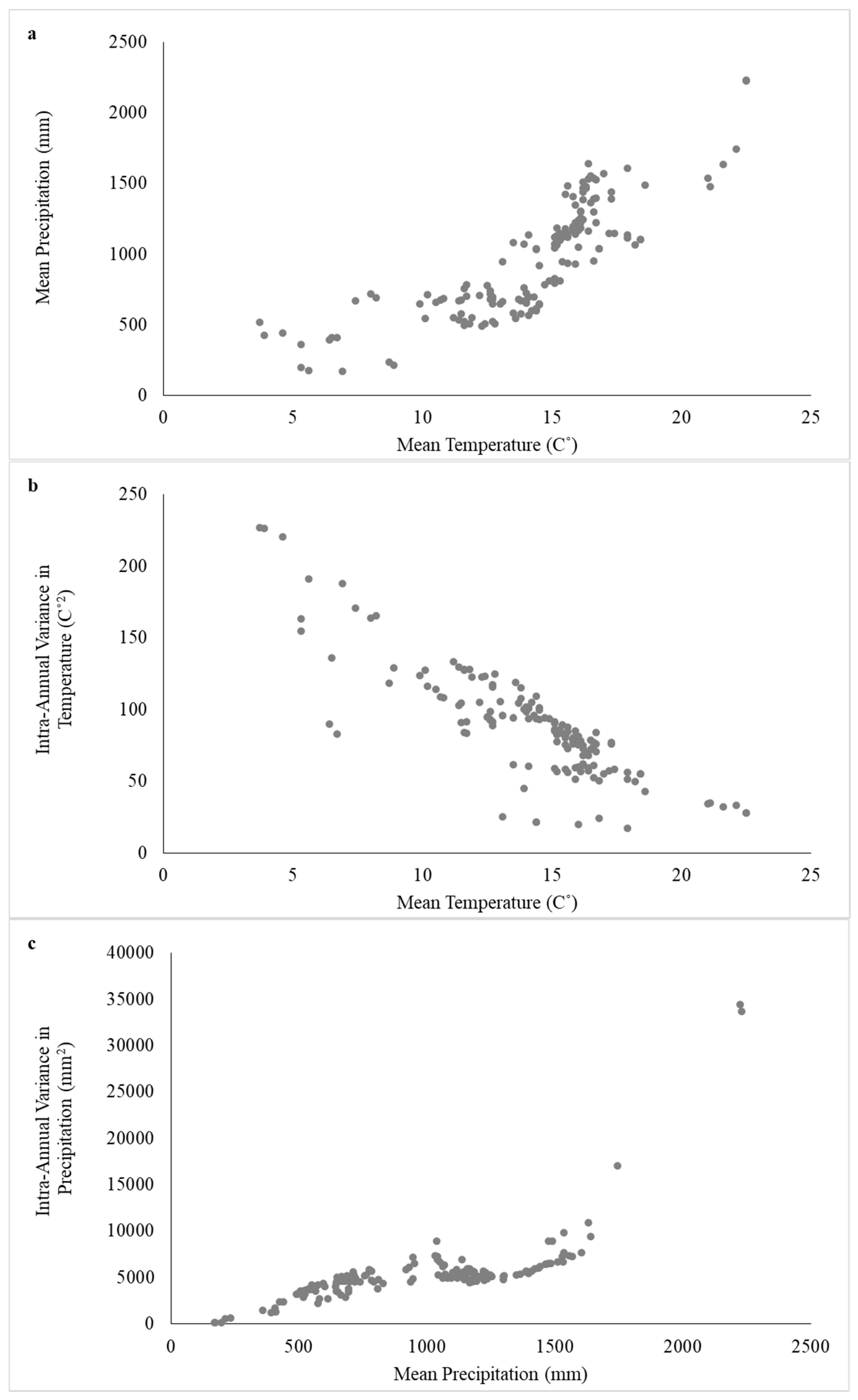
It appears from Table 3 that on average in our sample, between the establishment of a facility and the year 2006, temperatures have increased, and their distribution within the year has narrowed. Precipitation has declined on average and became less variable. Figure 1 depicts the spatial climate differences among the sample’s WWTP observations.
As can be seen in Figure 1, there is a very strong and well-defined relationship between the climatic characteristics of the WWTPs in the sample. Observations from high-temperature regions also are characterized by high precipitation levels (Figure 1a), lower variance in temperature within the year (Figure 1b), and higher variance in precipitation within the year (Figure 1c).
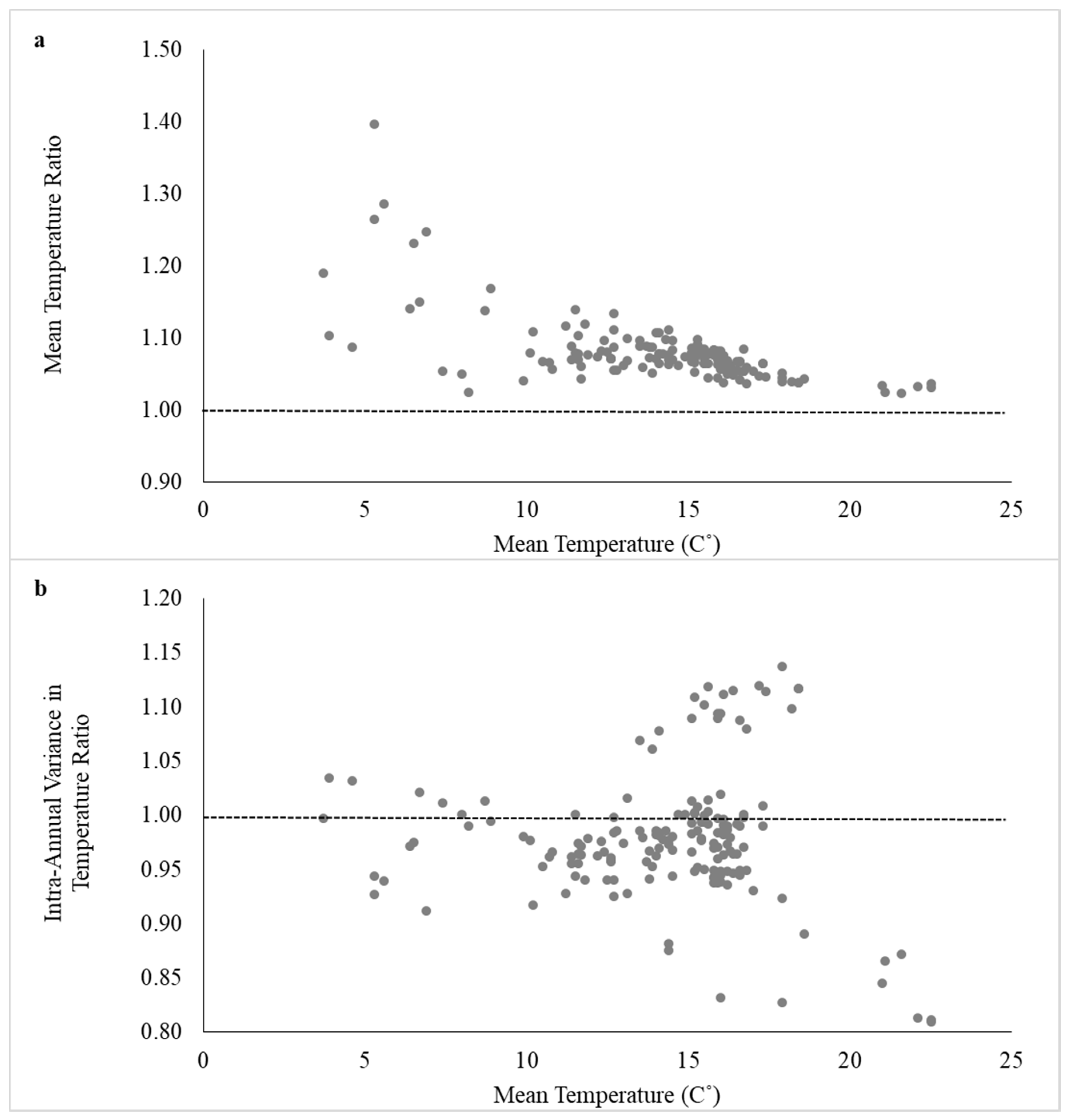
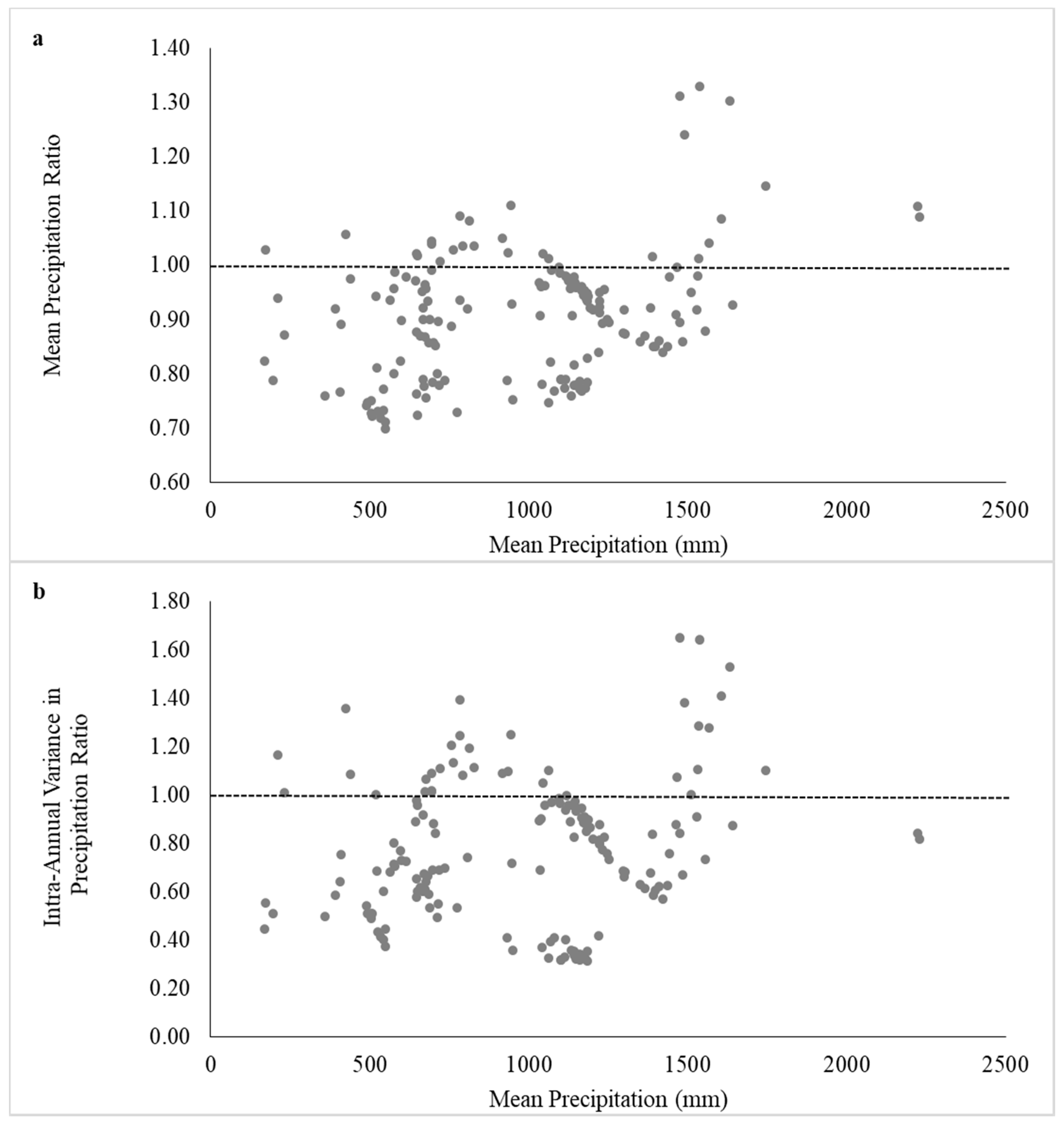
To examine the temporal trends of the climate variables in our sample, we compute for each such variable the ratio between the 2006 sample year value of that variable, and its historical average (normal). These ratios are presented in Figure 2 and Figure 3 as a function of temperatures and precipitation historical averages, respectively.
Figure 2 shows that all the treatment plants in the sample have experienced an average temperature increase with respect to the climate preceding their establishment, and that this increase was larger for plants in colder regions (Figure 2a). The variation in temperature within the year was mostly affected in warmer regions, where both higher and lower variation levels can be observed (Figure 2b). According to Figure 3, average precipitation levels generally decreased during the period of comparison, with some exceptions in the warmer and wetter regions (Figure 3a). The same can be said with respect to the intra-annual variation in rainfall (Figure 3b). Overall, while our sample accounts for only 16 percent of the WWTPs in China (in 2006), by examining Figure 1, Figure 2 and Figure 3 it can be concluded that our data adheres to the general climate trends in China, as well as to the regional climatic contrasts described in [42].
4. Methodology
The methodology in this paper comprises of an econometric estimation procedure of treatment costs of a wastewater sector, and a simulation of changes in these costs predicted with future climate conditions, policy implementation scenarios, population growth and development trends. The coefficients from the econometric estimation of the wastewater treatment sector cost function in the first stage are used in the simulation of future costs under various scenarios. The estimation of the treatment cost function includes, as explanatory variables, climate indicators at the plant level. This enables capturing the impact of changes in climate on costs of treatment, but also it allows distinguishing, as part of the simulation, between predicted costs when climate changes are accounted for, or ignored. Thus, providing an estimate of the opportunity costs associated with ignorant policy making with regard to climate changes impact on wastewater treatment costs. The estimation procedure and simulation model are described in general form in the following subsections.
4.1. Empirical Specifications
Following previous studies that estimated cost functions for wastewater treatment, we adopt a reduced form estimation approach, and assume a constant elasticity functional form relationship between costs of treatment and explanatory variables [43,44,45,46]. These assumptions are translated into an explicit definition of a cost function, as presented in general terms in Equation (1):
where are the total annual operating and maintenance (O&M) costs of the WWTP in the 2006 sample year, is a set of plant’s characteristics represented by dummy variables; is a vector of dummy variables representing the treatment technology of the plant, capturing differences in technology effectiveness; is a vector of dummies for the province where the plant is located, capturing provincial differences; and is a vector of variables indicating the decade at which the treatment plant was built, capturing technological improvements in recent decades. is the set of continuous determinants, where is the gross investment in the plant at the year of establishment (in 2006 constant dollars), is the average daily volume treated in the plant during the 2006 sample year, is the plant’s daily average treatment designed capacity, is a count of years since the establishment of the WWTP, and , and , are vectors of quality parameters and climate indicators, respectively. The ’s and ’s are the estimated parameters.
We include the investment in the treatment plant at the year of its establishment as a proxy for other design characteristics, such as area and other immobile capital associated with the treatment process. We expect this variable to have a positive and marginally decreasing effect on costs. Both volume of treatment and designed capacity are used in our analysis. Our hypothesis is that the closer the actual volume treated is to the designed capacity, the more cost-efficient the plant is. Regarding quality, we follow common practice in the literature on wastewater cost estimates and use biological oxygen demand (BOD) level as a single representative indicator for contaminants’ levels. This is also supported by professional literature suggesting that all the indices in our dataset (i.e., BOD, chemical oxygen demand-COD and total suspended solids-TSS) are closely related [40]. Our underlying hypothesis regarding the impact of climate on treatment costs is that each plant’s treatment efficiency is a function of its design. That design, in turn, is presumably a function of the prevailing climate in the region and the time at which the plant was built. Any changes with respect to that benchmark evident in the sampled period will affect the treatment efficiency and, consequently, the plant’s operating and maintenance costs.
While it has been argued that accounting for the differences between treatment technologies in the estimation of cost functions is important [47], studies that evaluated performance among WWTPs in different settings did not reach a consensus regarding the preferred technology in terms of cost efficiency [48,49,50].
Looking for examples to support the previous argument, we could find only esoteric treatment cost-estimation studies that addressed this issue. Reference [51], for example, compared capital and O&M costs of two treatment processes, namely up-flow anaerobic sludge blanket (UASB) and waste stabilization pond (WSP), among 25 WWTPs in the Yamuna River basin in India. Their findings suggest that the WSP is the cheaper technology of the two. Reference [52] focused their analysis on wastewater treatment costs in China. They concluded that chemical treatment processes are cheaper than biological ones. The authors have further classified biological treatment processes and indicated that anoxic-oxic (AO) has the lowest cost. To conclude, studying the literature concerned with the effect of different treatment processes on operating costs, we could not find any a priori justification for clear dominance of one technology over the other. To further strengthen this assumption, we refer to [53,54] who demonstrated that a combined processes approach, to achieve different treatment level goals, is the optimal cost-minimizing strategy.
We use the province dummies as both economic development indicators [52] and (in the absence of other documented classification) as indicators of the regulatory environment (i.e., effluent standards stringency) under which the plant operates. The decadal dummies account for technological differences (for example, older plants did not have access to technologies that were developed after their establishment).
In the next section we present the results of the ordinary least squares (OLS) estimates of Equation (2):
In Equation (2), all the continuous variables described earlier are expressed in natural-log form, and stands for the statistical error.
4.2. Simulation Procedure
The simulation is conducted in order to determine the magnitude of the impact of climate change on wastewater treatment costs predicted in the future, as well as estimating the cost of designing policy ignoring these impacts. For that purpose, the estimated coefficients from Equation (2) along with predicted values for variables in , and , are used to determine wastewater treatment costs in future time-periods under different sets of policy, climate, and wastewater volume scenarios. Let predicted values of climate indicators , for a future time-period (), be derived from a specific combination of a climate prediction model (), and greenhouse gas emission scenario (). Let the quality of wastewater be subject to regulation, and thus its value in future time-periods , an outcome of unique policy design (); and let the volume of wastewater in the future , be determined by projected trends of wastewater volumes (), derived from population growth, infrastructural development, and consumption behavior predictions. The predicted costs of wastewater treatment at the plant level can be defined as in Equation (3):
In Equation (3), and correspond to the vectors of explenatory variables defined in the previous subsection, where the values for explenatories depends on the combination of policy, climate and wastewater volume scenarios as described above. The set includes the coefficients ’s and ’s estimated from Equation (2). A unique simulation () then determines the inclusion or exclusion of variables in , and , as well as the choice of coefficients from , estimated under various specifications, used to predict under the combination of all future scenarios.
5. Estimation Results
We present in Table 4 the results of the estimated coefficients for Equation (2) under four specifications differentiated by the inclusion of control vectors. Column A corresponds to the estimation of Equation (2) excluding the vectors of provincial and decadal fixed effects. In column B, the estimated equation includes provincial dummies. Column C includes decadal fixed effects only, and column D includes both provincial and decadal fixed effects. The coefficients are presented along with their standard errors. Each specification’s adjusted R-Square, and the Moran I test statistic for spatial autocorrelation are also presented.
Similar to previous studies in this field, our results demonstrate that the sample’s cost function is characterized by economies of scale [43,44]. This could be realized based on the elasticity of costs with respect to the plant’s capacity, which is positive and lower than 1. The estimated coefficient for the investment variable shows similar sign and magnitude of the elasticity with respect to size, which suggests that operating costs also are characterized by scale economies with respect to other capital, which is beyond the correlation with the size of the plant. Volume treated, once capacity is controlled for, does not have a statistically significant effect on costs. The estimated coefficient of the tenure variable indicates the expected sign, suggesting that older plants would be more expensive to run. Yet, this effect is only statistically significant when decadal dummy controls are included in the estimation (Columns B and D). With respect to quality, our results indicate that the contamination level of the incoming flow (to the plant) is the important factor affecting the costs of treatment.
Moving onwards to discuss the impact of climate change on treatment costs, it is important to emphasize again that the variables used are the historical average temperature and intra-annual variance in temperature (normal), and the ratios between the sample year-observed-weather for the same variables and their historical counterparts. This means that the effect of past average temperature (intra-annual variance in temperature) actually equals the difference (). Whereas and correspond to the effects of the sample year observed values of average temperature, and the variance in temperature within-year, respectively. (The statistical significance of the difference coefficient is determined based on a test performed after the estimation. Results of these tests correspond to the significance level derived from the coefficients and standard errors of and , reported in Table 4, for average temperature and intra-annual variance, respectively.)
Our choice of including temperatures alone is justified in several ways: First, based on the strong biological connection between temperature and treatment efficiency as presented in the scientific literature review provided earlier. Second, given the current conditions of the wastewater collection systems in China [28], the precipitation effects discussed in the same literature review are less likely to occur. Third, the strong relationship between temperature and precipitation patterns in our sample (Figure 1) introduces multicollinearity when both types of variables are included in the model.
The estimation results support our earlier hypothesis. Historical within-year variance in temperatures has a negative and statistically significant coefficient at the 1 percent level. This implies that a plant designed to operate under higher past temperature variance (keeping, among all other variables, the 2006-observed within-year variance constant) is cheaper to run in 2006—the year of the sample. The coefficient for the sample year’s intra-annual variance in temperature is positive and significant at the 1 percent level. This corresponds to the effects of weather extremes that are beyond the designed capacity of the plant. The interpretation is that the operating cost of a treatment plant that at the time of its establishment experienced a 10 percent higher within-year temperature variance than the sample average, is lower by 18.4 percent (according to the coefficient in column A of Table 4). Whereas an increase of 10 percent in observed within-year variance of a plant leads to an increase of almost 22 percent (column A in Table 4) in variable treatment costs. Coefficients of average temperatures (observed in 2006, and historical normal) are not statistically significant but do have intuitive signs.
Regarding treatment technologies, some findings from previous studies [52], on which we reported earlier, are also partially supported by our results (i.e., cheaper operations when using AO treatment technology). However, as a general conclusion and in-line with the existing literature, we cannot point to a specific technology as being cost preferred over another. The only consistently significant coefficient in our results belongs to the group of plants defined “Not Specified.” This group consists of two plants whose reported technology specification made it impossible to assign to any of the other technology groups. We also estimated the model without these two observations; this experiment did not yield any significant improvements to the reported results.
Our attempt to control for economic development or standards stringency through the inclusion of provinces’ dummy indicators did not yield meaningful results. This is due to high multicollinearity between provinces and climate, which also influences the latter’s statistical significance (Column B of Table 4). As can be found in [55], provinces are almost completely homogenous in climate attributes, and are divided almost exclusively between China’s climate zones [55] (Figure 1). Interestingly, for the log-linear functional form, the estimation presented in Appendix A Table A1 (Columns 4 and 5), including the provincial dummy variables did not yield the same outcome (i.e., the coefficients for historical and the sample year intra-annual variance in temperatures, which is of similar signs to the coefficients presented in Table 4, remained significant at the 1 percent level). Obviously, this implies that our results are sensitive to the functional form choice. Yet, it also demonstrates that the cost impact of changes in climate we observed in our estimation is not only attributed to climatic differences across provinces in China, but rather also to spatial differences in climate changes between plants from the same province. The latter conclusion supports our earlier argument of multicollinearity, which stems from variables definitions, in favor of a systematic bias associated with excluding time-variant and -invariant determinants from the estimation that are captured by provincial differences.
Next, we address several important econometric issues. First, we find our estimation results robust to the introduction of sampling weights as calculated based on differences presented in Table 2 (see Appendix A Table A2 for comparison). With respect to the choice of functional form, while we chose the constant elasticity form to represent the technology based on common practice in the field, other alternatives should also be considered. Using the Ramsey (RESET) specification-error test [56], we could not exclude either the linear form or the log-linear form as compatible models. Nevertheless, we find that the results from all three functional form models are qualitatively non-distinguishable. We also test our model for endogeneity with respect to the concentration of BOD in effluents, which can be thought of being subject to managerial decisions. The results of these tests could not reject the null hypothesis that this variable is exogenous (see Appendix A Table A3). The Moran I test for the existence of spatial autocorrelation in error terms is mostly rejected, except for one specification. For that specification (Column C in Table 4), coefficients are estimated using a maximum likelihood procedure. However, the results of that estimation, as presented in Table 4, do not differ significantly from the alternative specifications. Lastly, we perform several robustness checks to our model (not reported). These include replacing average temperature with minimum and maximum temperature variables, controlling for larger climatic regions instead of provinces, and inclusion of the different combinations of control vectors (i.e., decadal dummies, provincial dummies, and climatic regions dummies) in different functional form specifications—as those are described in Appendix A Table A1.
In the next section we demonstrate the use of the estimated WWTP cost function through several simulations of different policy scenarios under various climate change predictions, using the estimated coefficients presented in Table 4.
6. Simulations of Future Policy Impacts
We start this simulation exercise with a short discussion of possible future scenarios and projections of important factors to be considered in the analyses. First, with respect to future policy scenarios, given the literature reviewed, and specifically with respect to the Chinese case analyzed earlier, we choose to focus on treated wastewater discharge standards as the future policy intervention. Over time, and as wastewater reuse becomes more widespread, one can observe increased levels of regulatory policies using more stringent quality standards for treated wastewater disposal [57]. Quality standards, especially one-quality-fits-all, are applied as the policy intervention to protect human health and the environment. The policy question that has been discussed in the literature addresses the tradeoff between increased cost of treatment and the level of stringency of the quality standards [39,58]. In the context of the China case, several works identified that quality standards for treated wastewater discharge should be amended, and that future policies should be designed to confront China’s growing water quality issues in general [30,36,59].
6.1. Climate Predictions
The simulation horizon starts in 2020 and ends in 2100 and is divided into three equal 27-year periods. For climate change predictions, we use projections from the Coupled Model Inter-Comparison Project (CMIP5) database [60]. Following previous literature that addresses climate change in China [61,62], and given potential sensitivity of simulation results to the use of predictions from a specific climate change model [63], we try to account for a wide range of future predictions in our analysis. For that purpose, we use projected climate from seven different global circulation models (GCMs) selected from the ensemble reviewed by [62] (we decided not to use the model FGOALS-s2 [64], since it did not have predictions for RCP 2.6 and RCP 4.5. The other three GCMs we are not using predict that annual average temperatures will drop below their observed levels in our sample (in 2006), under all RCPs). For each of the selected models, predictions of future climatic conditions are derived from three greenhouse gas emission scenarios, which are also known as representative concentration pathways (RCPs).
For all chosen GCMs, we collected monthly near-surface temperature data from the CMIP5 database. We then computed, for each of the three future periods, 27-year average values for the annual average and intra-annual variance in temperatures (The results from these robustness checks did not yield significantly different results to the ones presented herein and are therefore not presented for the sake of brevity, but are available from the authors upon request. We also collected monthly precipitation data and computed the same variables as we did for temperature. We use these computed variables to corroborate the assumption that the relationship presented in Figure 1 prevails also for the predicted future climate. Excluding MIROC-ESM and MIROC-ESM-CHEM climate predictions from all models support this assumption.). As before, we fit the predicted climate variables for each observation in our sample using the IDW method. following common practice in this field [62,65], all GCMs data were uniformly interpolated to identical resolution (0.5° × 0.5°) using bilinear interpolation prior to fitting the data to each observation in the sample. The temperature predictions for each model under all RCPs and for each of the future periods is presented in Table 5.
According to Table 5, the models can be roughly grouped, based on their future predictions, to fit different temperature trajectories. In terms of annual average temperatures, one group of models (CanESM2, MIROC5, MIROC-ESM and MIROC-ESM-CHEM) is generally more expanding (i.e., predicts larger temperature increases) than the other more moderate group of models (BCC-CSM1, GISS-E2-R and MPI-ESM-LR). In terms of intra-annual variance in temperatures, most models are grouped together and present only small changes with respect to the base period. Whereas, two models predict moderate (MPI-ESM-LR) and sharp (GISS-E2-R) decrease in within-year variance. Models also can be distinguished by their future trends; however, such a distinction is much finer and depends on the RCP scenarios.
6.2. Policy Scenarios
As mentioned, we choose to focus on treated wastewater discharge standards as our policy scenario. In that respect and given the literature reviewed earlier, we simulate a homogeneous quality standard requiring all plants in our dataset to treat wastewater to Class 1A as defined by the national standard for treated wastewater discharge (GB 18918–2002). We assume that inflow quality to each plant remains at the observed level throughout the simulation exercise. Thus, this policy implies a further reduction of at least 50, 67, and 83 percent in effluents’ BOD level for 49, 32, and 11 percent of the WWTPs in our sample, respectively. As mentioned earlier, we aim to analyze a wide range of scenarios in this simulation exercise. This, in turn, will allow us to provide cautious estimates toward the usefulness of our approach, i.e., estimating the opportunity costs associated with ignoring future climate change impacts on wastewater treatment. Since our simulation is conducted on future predictions, we also try to account for possible trends in other important variables, specifically wastewater volumes. Obviously, such future aspects introduce higher level of uncertainty, and predicted trajectories will be determined by a combination of multiple factors. We therefore concentrate on measurable factors and supporting literature in order to construct several meaningful scenarios. With respect to factors to be considered, wastewater volumes should be a function of domestic and industrial water consumptions, and the rates of sewage generated, collected, and conveyed to treatment facilities.
Following the literature concerned with modeling future water consumption in China [66,67], we consider the following factors in constructing our scenarios: (a) population growth, (b) per-capita water consumption, and (c) urbanization rates. For population trajectories, we rely on the “high-variant” and “low-variant” scenarios taken from the population division of the United Nations [68]. Per-capita water consumption and urbanization rates are more elusive factors in terms of future predictions. We therefore assume for both either linear trends of continuous growth, based on documented recent historical trends in China, Reference [66] for urbanization; and [32] for per-capita water consumption, or no change at all, throughout the duration of the simulated horizon. Finally, the population connected to sewage systems and centralized treatment facilities in China is approximately 80 percent in urban areas, and far lower in rural ones [69]. Whether centralized or decentralized, treatment systems will be characterizing future development and, in turn, influencing these shares is still unknown [69]. We therefore assume either linear trends throughout the horizon or no change for this factor as well.
Based on all possible combinations of the aforementioned factors, we construct multiple trajectories from which we picked six, representing a wide range of possible wastewater volume development paths. These trajectories are presented in Figure 4 and labeled V1 through V6. According to Figure 4, an increasing trend characterizes V1 through V3. In V1 scenario, wastewater volume increase is of an exponential form, V2 demonstrates a more moderate growth projection of wastewater volumes, and V3 predicts only a slight increase in wastewater volumes throughout the century. Scenarios V4 and V6 demonstrate a decreasing trend in predicted wastewater volumes, with V4 being the more conservative prediction. According to V5 scenario, wastewater volumes are expected to increase until the middle of the century, and then decline back almost to their original observed level. We also construct three policy scenarios, based on the future period in which our hypothetical treated wastewater discharge policy standards will be implemented (i.e., in the short, medium, or long term). We label these scenarios as P1, P2, and P3 for short-term, medium-term, and long-term implementation scenarios, respectively. We also notate as R1, R2, and R3 the three RCP scenarios, RCP 2.6, RCP 4.5, and RCP 8.5, respectively. Our seven GCMs are labeled G1 through G7 according to their order of appearance in Table 5.
We conduct three separate simulations, and in each the set of relevant variables is adjusted to its projected values according to the scenarios described above. The treatment cost in each simulation is predicted based on the different estimated functions as they are prescribed in the following description. The first, labeled “Sim1,” is carried using the coefficients estimated in the previous section. Being conservative, we use the coefficients from Model B (Table 4, Column 3) accounting for provincial differences. For each combination of policy scenario (P0 through P3) and wastewater volume trajectory (V0 through V6), we simulate all combinations of GCMs and RCPs for each of the three future periods(P0 and V0 are the scenarios in which volume and discharge standards remain at their base-year observed levels throughout the duration of the simulated period.) For the second simulation (Sim2), we project impacts on costs of treatment from future policy scenarios and wastewater volume changes alone, keeping climate variables at their observed 2006 values. Similar to Sim2, in the third and final simulation (Sim3) we calculate only the impact of policy scenarios and volume projections’ combinations on the cost of treatment. However, for this last simulation we use a new set of coefficients, i.e., we estimate the cost function model presented in Equation (2); however, dropping from the estimation the climate variables (see Appendix A Table A4). This set of coefficients is used to simulate the changes in costs when all possible climate impacts (direct and indirect) are ignored.
Using results of all three simulations, the impact of future predictions with respect to climate change on treatment costs can be broken down into two parts. The first part, represented by the difference in treatment costs between Sim1 and Sim2 is the impact of predicted climate change alone (both use the same set of coefficients but differ in the values of climate variables used for predicting costs of treatment). Whereas, the difference in treatment costs between Sim2 and Sim3 is attributed only to the inclusion of climate change in the estimation exercise (in both of these simulations, climate remains unchanged however, different sets of coefficients are used for predicting treatment costs). It is measured by the cost impact derived from changes to the coefficients of the cost function determinants other than climate. These changes, in turn, are the result of including the climate variables in the estimation.
Under all three simulations, we compute the O&M costs, , for each plant
in our sample (). Based on that calculation, we can also compute the average treatment cost per unit of water treated at the plant level (
), and the total annual O&M costs for the entire sample, (where ). For both cost measures, we compute average (, ), min (, ), and max (, ) values for the sample.
6.3. Simulation Results
We turn now to describe the results of our simulation analysis. First, we report the results from Sim1, which is the total predicted effect of climate change on treatment costs. Table 6 presents the predicted levels of , and , in present-value terms, for all RCPs and for each of the GCMs, averaged over policy and volume change scenarios. The discount rate for calculation of present values is assumed to be 3 percent (acknowledging the literature discussion regarding assumed discount rates in [70], we also use discount rates of 1.4 and 5.5 percent).
It can be seen from Table 6 that for most models and for different RCP scenarios, costs of treatment are expected to increase as a result of climate change. The reason is the positive and relatively large values of estimated coefficient for the change with respect to past climate of the intra-annual temperature variation (Table 4, Row 10). According to most models that variable is predicted to increase over time (Table 5). The exceptions are models G3 and G7, which as noted earlier, predict a decrease in the within-year variation in temperatures compared to the historical climate. According to Table 6, the impacts on total annual costs over the sample range between an increase of 19 percent and a decrease of 75 percent, at the extremes. The changes predicted in annual O&M costs for the average plant in the sample are the same. Average costs for a unit of water treated ranges according to the simulated predictions between a 46 percent increase and 75 percent decrease. As the predicted changes in climate generally expand with time, the use of lower discount rate magnifies these outcomes such that costs are expected to increase with respect to the base year under all models except G3. The changes in total annual costs over the sample and for an average plant, based on the lower discount rate calculations, are within 156 percent increase to a decrease of 45 percent. Average cost for treated unit of water ranges between a 229 percent increase and 41 percent decrease. Using a higher discount rate reverses the relationship such that costs under all models and RCP scenarios decrease with respect to the base year. Total and average annual O&M costs changes range between a decrease of 55 to 91 percent. Average cost per unit of water treated also decreases in the range of 47 to 91 percent.
Table 7 reports, for the various cost measures, the differences between Sim2 and Sim3 as well as differences between Sim1 to Sim3, on average, across all models and scenarios. The ratio of these two differences, which is also reported in Table 7, can be interpreted as an estimate of the opportunity costs associated with ignoring climate change impacts on treatment costs. As noted earlier, it is the share of cost impact derived from changes to all other coefficients in the estimated cost function (except for the climate coefficients), when climate variables are also included in it, and while keeping climate unchanged with respect to the observed values in the 2006 sample year. When in the range of 0 to 100, a higher ratio indicates a better prediction of the opportunity cost simulated by the impact of climate. A ratio outside of that range indicates a poor prediction of the simulated impact of climate, where it is either an overestimation (ratio over 100) or suggests an estimate in the opposite direction (negative ratio) of the projected impact.
The ratios presented in Table 7 suggest that for an average plant in the sample (and for the entire sample), 46 percent of the impact on annual O&M costs predicted by Sim1 with respect to Sim3 is attributed to all other factors considered in the estimation except climate. As explained above, this partial impact is manifested through changes in estimated coefficients resulting solely from the inclusion of climate variables in the estimation procedure. For the average treatment cost per unit of water, , the ratio is 33 percent, suggesting a slightly lower predicted impact of that opportunity costs estimate. On average, the cheapest plant in terms of both annual and per unit of treated water O&M costs appears almost unaffected by climate change. This means that the inclusion of climate variables in the estimation attributes an increase in costs (i.e., the difference between Sim1 to Sim2), which disappears (and even reverses) when climate effects themselves are accounted for (i.e., the difference between Sim1 to Sim3). The highest impacts predicted by climate change simulation across our sample seem to be only weakly or moderately explained by the inclusion of climate variables in the estimation alone.
Table 8 presents the same ratio that was presented in Table 7 across the range of GCMs and RCPs. Given that calculation of the ratio of differences in annual O&M costs is identical for an average plant and for the total annual costs over the entire sample, we report henceforth just on the former.
According to Table 8, the portion of climate change effects on wastewater treatment costs, which is associated with inclusion of climate variables in the estimation, ranges between 23 to 41 percent, and from 17 to 25 percent for the annual O&M costs of an average plant, and for average cost of unit of water treated, respectively. The exceptions are the G3 and G7 models, in which the cost impact predictions based on that ratio are either overestimated or in the opposite direction of the simulated impact resulting from the models’ projections. The ranges for these ratios when calculated based on high (low) discount rate are 21 to 41 (24 to 42) percent, and 15 to 24 (18 to 25) percent, for and , respectively.
Turning to examine variation in the results from a different perspective, Table 9 presents the same ratio between differences in costs across volume and policy scenarios.
Looking across volume and policy scenarios, the share of annual O&M costs’ impact from climate change associated with the estimation alone ranges between −128 and 37 percent. In the majority of scenarios, the simulated impact from climate change and the opportunity cost estimates are predicted to have opposite signs. For the average cost of unit of water treated that ratio ranges between 45 and 122 percent—with most scenarios predicting a lower ratio than 100 percent. Calculating the variation of ratios using high (low) discount rate, we find that ranges between −19 to 43 (−214 to 2872) percent, and ranges between 51 to 291 (42 to 192) percent, respectively.
To summarize, the results of the simulation analysis suggest that climate change impacts on wastewater treatment costs can be substantial. The estimate we calculated for the opportunity cost associated with ignoring these potential effects is also quite significant. Depending on assumed discount rate, we find that variation of the opportunity costs estimate among policy implementation scenarios, given uncertain future development, could be substantial as well. Yet, depending on predicted changes in climate from different GCMs, in some cases climate effects will decrease or even reverse the predicted impacts resulting from the educated estimation alone. For the former, the cost of ignoring climate change might be negligible. These cases; however, are the minority according to the results of our analysis.
7. Conclusions and Policy Implications
A higher number of wealthy people living in urban areas results in increased pressure on water resources and the environment. On the one hand this means an increased demand for water and higher level of sewage generation that necessitates treatment to reduce health risks and environmental damage. On the other hand, treated municipal wastewater is a source of stable and good-quality water supply. However, the benefits of that additional, reliable source of water is affected by the wastewater collection, treatment, and disposal, which are all capital- and energy-intensive processes. This makes treatment necessity an expensive social dilemma that must be addressed by proper public policy. The result of such a dilemma, which is associated with public budget tradeoff, is that the majority of developing countries still do not treat wastewater, whereas countries in the developed world face, at different magnitudes, challenges associated with economic efficiency of the treatment investments and disposal of wastewater sub-quality.
Uncertainty in future climate only intensifies this dilemma. The impacts associated with climate change may have contradicting effects on the social costs of wastewater treatment. While reoccurring droughts, dry and warm conditions encourage the potential use of treated wastewater as a substitute to natural fresh water for beneficial uses, higher frequency of extreme climate-related events, such as floods, cold or hot weather might impair the efficiency of the treatment process, making it much more expensive and less effective. Being within the public good domain (or public bad, as stated by [71]), wastewater-related activities are usually characterized by some level of centrality, making them more susceptible to policy interventions. However, in order to conduct the social cost-benefit analysis the climate-related potential impacts must be quantified. The current paper therefore takes a first step toward a better understanding of the impact of climate change on actual operating costs of wastewater treatment and, ultimately, on the ability of societies to cope with increased water scarcity and water quality risks.
We estimate an average cost function for a cross-section sample of the wastewater treatment sector in China, and we use the estimated coefficients to simulate impacts of future climate changes on the costs of treatment. While the analysis in this paper uses data from China, the approach we use could be applied to any country or region from around the world where data might be available. This approach offers the ability to assess several policy interventions that could be considered by regulatory agencies in order to sustain the wastewater treatment sector.
While relatively simplistic, our analysis offers some important insights. The econometric estimation results corroborate our a priori assumption regarding climate effect, i.e., materialized extremes that lie outside of the distribution of climate measures observed at the time the WWTP was designed are estimated to significantly alter the cost of treatment. Therefore, climate must be accounted for when wastewater treatment processes are designed, and their costs and performance are studied. The simulation analysis points to three noteworthy results and their derived conclusions. First, based on most climate predictions used in the analysis, costs of wastewater treatment are expected to rise with the effect diminishing and even reversed as assumed discount rates increase. This, in turn, demonstrates the importance of quantifying uncertainty and measuring the magnitude of its impact, which in our case is quite large. Second, keeping climate stationary, our estimate of the opportunity costs associated with ignorance of these potential impacts can be fairly significant, emphasizing our earlier conclusion regarding the inclusion of climate in future analyses. Third, when comparing across policies, ignoring climate change impacts on future planning of wastewater treatment could have different estimated opportunity costs, suggesting that information on future climate change impact could be critical for efficient policy design.
Finally, our analysis can benefit from several future extensions. First, increasing the sample size, spatially and temporally, provides the opportunity to identify and statistically interpret each of the individual effects we studied in a more robust manner. Second, as suggested in relevant literature [44,72,73], some variables within the wastewater treatment domain might be endogenous and determined by some type of equilibrium process. This suggests that a structural approach could be relevant, which can either corroborate or reject the underlying theory. Another strand of the literature in this field is focused on measuring relative performance and using it to identify factors that can contribute to efficiency gains [49,50,74,75]. Both of these approaches could generate important insights to the social dilemma we analyzed, but would require a larger dataset, including a wider range of observations and control variables, than the data used in our study. Lastly, our results rely on a cross-section estimation, a methodology that is commonly criticized for omitting important time-variant and -invariant variables. This can obviously lead to biased estimates. While this problem is partially solved by introducing provincial dummy variables, still caution should be taken when interpreting the results. Consequently, any future analysis should preferably use panel methods and expand the range of determinants when trying to identify climate impacts on treatment costs.
Supplementary Materials
The following are available online at https://www.mdpi.com/2073-4441/12/11/3272/s1, Table S1: Simulated future climate change impacts on wastewater treatment costs under 1.4% interest rate assumption; Table S2: Simulated future climate change impacts on wastewater treatment costs under 5.5% interest rate assumption; Table S3: List of symbols used in the manuscript.
Author Contributions
Conceptualization, A.R. and A.D.; methodology, A.R.; validation, A.R., A.D. and Y.J.; formal analysis, A.R.; investigation, A.R., A.D., Y.J.; resources, A.R., A.D.; data curation, A.R., Y.J.; writing—original draft preparation, A.R.; writing—review and editing, A.D., Y.J.; supervision, A.R., A.D. All authors have read and agreed to the published version of the manuscript.
Funding
This research received no external funding.
Acknowledgments
We would like to thank Yixing Sui from the University of Antwerp and Teng Li from Sino-French Water Development for their insightful contributions in the early stages of this study. Ami Reznik acknowledges the support of the Vaadia-BARD Postdoctoral Fellowship (No. FI-563-2017). Yu Jiang would like to acknowledge the support from Climate-KIC and to thank Yuan Liu for her help with some of the data entry. Ariel Dinar would like to acknowledge support from the W4190 Multistate NIFA-USDA Project, “Management and Policy Challenges in a Water-Scarce World.”
Conflicts of Interest
The authors declare no conflict of interest.
Appendix A. Different Cost Treatment Model Specifications
In this appendix, we describe the outcomes of different specifications for the cost function estimation procedure. In Table A1 we present the results of several alternative functional forms for the underlying technology. Table A2 shows the outcomes of estimating the model while accounting for sampling weights based on different calculations. In Table A3 we report the second stage results from an instrumental variable estimation procedure performed to test for endogeneity of the level of BOD in effluents, along with the tests’ statistics. The instrumental variables used for these estimations are the level of COD and TSS in the plant’s effluents. Table A4 reports the results of estimating the cost function in a Cobb-Douglas form, excluding climate variables. The coefficients from that estimation are the ones used in the simulation exercise for Sim3. All the results presented in the tables below are based on estimations that do not include any fixed effects, and therefore should be compared against Column A in Table 4. The exception is Table A4, in which provincial dummies are used, and so the coefficients from that table should be compared to Column B of Table 4. We do not report the coefficients for treatment technologies in the tables below for brevity considerations.

Table A1.
Different functional form specifications.
| Variable\Model | (1) | (2) | (3) | (4) | (5) |
|---|---|---|---|---|---|
| Investment () | 0.518 (0.133) | 0.006 (0.003) | 0.011 (0.005) | 0.273 (0.069) | 0.287 (0.070) |
| Capacity () | 1.168 (0.327) | 0.056 (0.026) | 0.199 (0.039) | 0.523 (0.166) | 0.504 (0.169) |
| Volume () | −0.276 (0.293) | −0.004 (0.028) | −0.078 (0.042) | −0.050 (0.149) | −0.034 (0.150) |
| Tenure () | −0.231 (0.166) | 0.009 (0.009) | −0.014 (0.013) | 0.120 (0.083) | 0.002 (0.007) |
| Quality Parameters | |||||
| BOD Influent () | 0.313 (0.152) | 0.001 (0.001) | 0.001 (0.001) | 0.170 (0.078) | 0.186 (0.078) |
| BOD Effluent () | −0.147 (0.124) | 0.001 (0.007) | −0.003 (0.010) | −0.014 (0.063) | −0.023 (0.063) |
| Climate Indicators | |||||
| Hist. Mean Temp. () | −0.485 (0.441) | 0.008 (0.030) | −0.017 (0.045) | 0.004 (0.026) | 0.002 (0.026) |
| Hist. Intra-Ann. Temp. Var. () | 0.053 (0.265) | 0.006 (0.003) | 0.003 (0.004) | 0.004 (0.002) | 0.004 (0.002) |
| Mean Temp. Ratio () | −0.128 (2.845) | −1.517 (1.446) | −1.279 (2.132) | −0.765 (1.201) | −0.53 (1.207) |
| Intra-Ann. Temp Var. Ratio () | 1.620 (1.609) | 1.798 (0.905) | 2.031 (1.335) | 2.782 (0.814) | 2.305 (0.771) |
| Constant Term | −0.190 (2.164) | −1.044 (2.190) | 0.425 (3.230) | −4.438 (1.891) | −4.035 (1.883) |
| Adjusted R2 | 0.599 | 0.506 | 0.675 | 0.650 | 0.646 |
| Ramsey (3,142) | 16.099 | 12.231 | 1.150 | 1.879 | 1.751 |
Notes: Values in parenthesis are estimated standard errors.
Table A2.
Cost function estimation results using different sampling weights.
| Variable\Model | (1) a,c | (2) b,c | (3) a,d | (4) b,d |
|---|---|---|---|---|
| Investment () | 0.231 (0.081) | 0.275 (0.066) | 0.259 (0.066) | 0.232 (0.083) |
| Capacity () | 0.481 (0.224) | 0.464 (0.201) | 0.497 (0.19) | 0.486 (0.214) |
| Volume () | −0.022 (0.200) | −0.040 (0.181) | −0.054 (0.172) | −0.066 (0.192) |
| Tenure () | 0.042 (0.118) | 0.046 (0.107) | 0.095 (0.109) | 0.102 (0.132) |
| Quality Parameters | ||||
| BOD Influent () | 0.097 (0.115) | 0.119 (0.105) | 0.139 (0.105) | 0.108 (0.119) |
| BOD Effluent () | −0.015 (0.064) | −0.015 (0.058) | −0.039 (0.051) | −0.035 (0.061) |
| Climate Indicators | ||||
| Hist. Mean Temp. () | 0.120 (0.200) | 0.103 (0.196) | 0.173 (0.194) | 0.137 (0.242) |
| Hist. Intra-Ann. Temp. Var. () | 0.456 (0.099) | 0.401 (0.092) | 0.471 (0.105) | 0.459 (0.109) |
| Mean Temp. Ratio () | −0.149 (1.415) | −0.005 (1.469) | −0.257 (1.168) | 0.171 (1.715) |
| Intra-Ann. Temp Var. Ratio () | 2.326 (1.29) | 2.436 (1.134) | 1.907 (1.055) | 2.650 (1.183) |
| Constant Term | −3.693 (0.773) | −3.609 (0.757) | −4.251 (0.748) | −3.851 (0.905) |
| Adjusted R2 | 0.649 | 0.650 | 0.685 | 0.634 |
Notes: Values in parenthesis are estimated standard errors.; a Calculation of weights is based on information from [36]; b Calculation of weights is based on information from [35]; c Calculation of weights is based on number of represented plants in the industry; d Calculation of weights is based on the share of treatment technologies in total capacity of the industry.
Table A3.
Instrumental variables regression for identifying endogeneity, different estimation methods.
Table A3.
Instrumental variables regression for identifying endogeneity, different estimation methods.
| Variable\Model | 2SLS | GMM |
|---|---|---|
| Investment () | 0.265 (0.066) | 0.267 (0.058) |
| Capacity () | 0.564 (0.158) | 0.557 (0.168) |
| Volume () | −0.091 (0.142) | −0.085 (0.159) |
| Tenure () | 0.076 (0.081) | 0.073 (0.095) |
| Quality Parameters | ||
| BOD Influent () | 0.173 (0.081) | 0.175 (0.098) |
| BOD Effluent () | −0.049 (0.129) | −0.048 (0.115) |
| Climate Indicators | ||
| Hist. Mean Temp. () | 0.088 (0.212) | 0.087 (0.165) |
| Hist. Intra-Ann. Temp. Var. () | 0.383 (0.133) | 0.379 (0.099) |
| Mean Temp. Ratio () | −0.728 (1.371) | −0.714 (1.017) |
| Intra-Ann. Temp Var. Ratio () | 2.174 (0.777) | 2.175 (0.953) |
| Constant Term | −3.769 (1.039) | −3.762 (0.694) |
| Endogeneity Test (H0: Variable is Exogenous) | ||
| Durbin score (2SLS)/GMM C (GMM): | 0.029 | 0.034 |
| Wu-Hausman (2SLS): F(1,144) | 0.025 | |
| Overidentification (H0: No Overidentification) | ||
| Sargan score (2SLS)/ Hansen’s J (GMM): | 0.020 | 0.029 |
| Basmann (2SLS): | 0.017 | |
| Adjusted R2 | 0.659 | 0.659 |
Notes: Values in parenthesis are estimated standard errors.
Table A4.
Constant elasticity functional form without climate variables (used for sim3).
| Variable\Model | Coefficients |
|---|---|
| Investment () | 0.148 (0.068) |
| Capacity () | 0.715 (0.164) |
| Volume () | −0.109 (0.143) |
| Tenure () | −0.063 (0.079) |
| Quality Parameters | |
| BOD Influent () | 0.177 (0.078) |
| BOD Effluent () | −0.044 (0.063) |
| Constant Term | −1.348 (0.565) |
| Adjusted R2 | 0.714 |
Notes: Values in parenthesis are estimated standard errors.
Appendix B. Observed and Predicted Climate in China
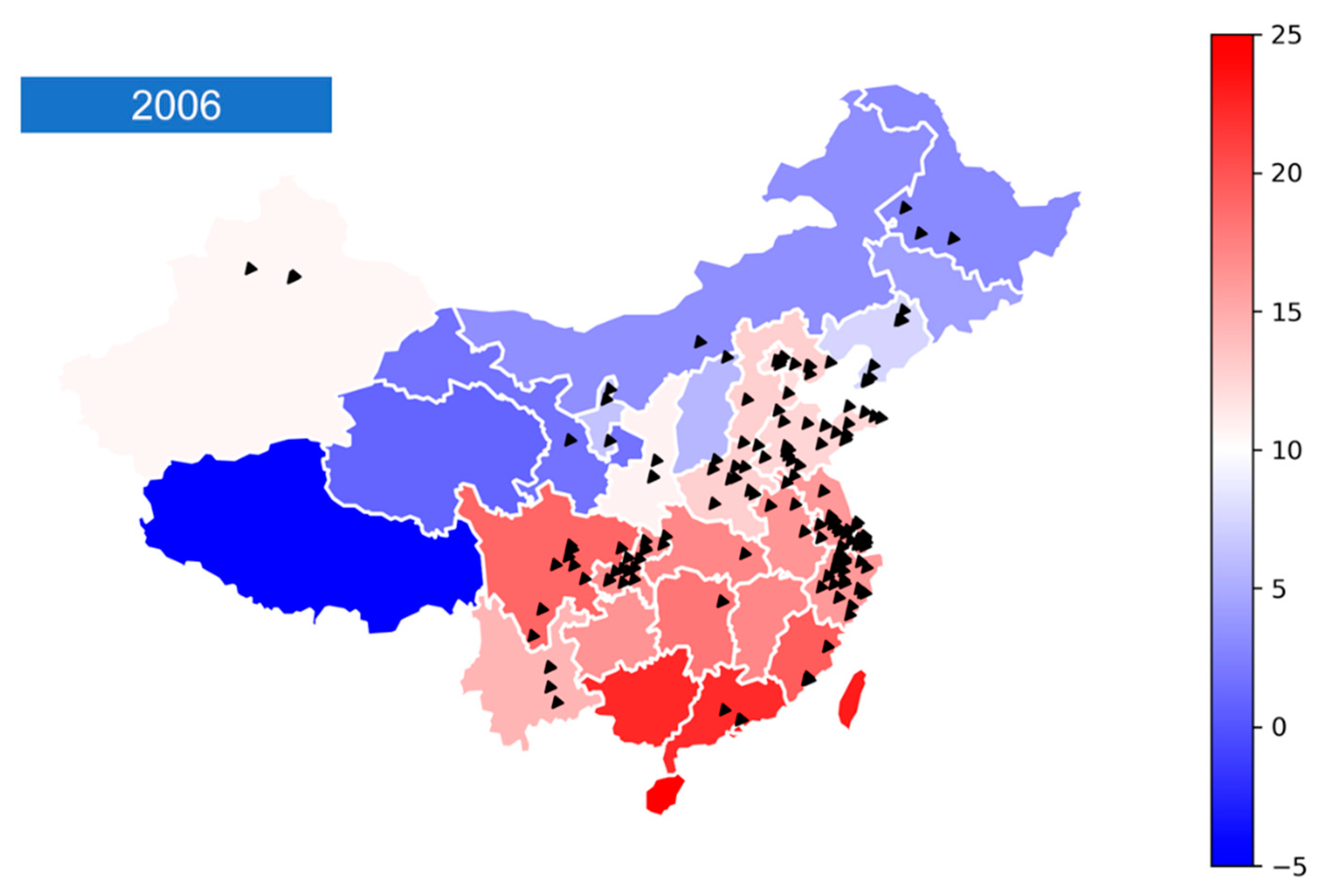
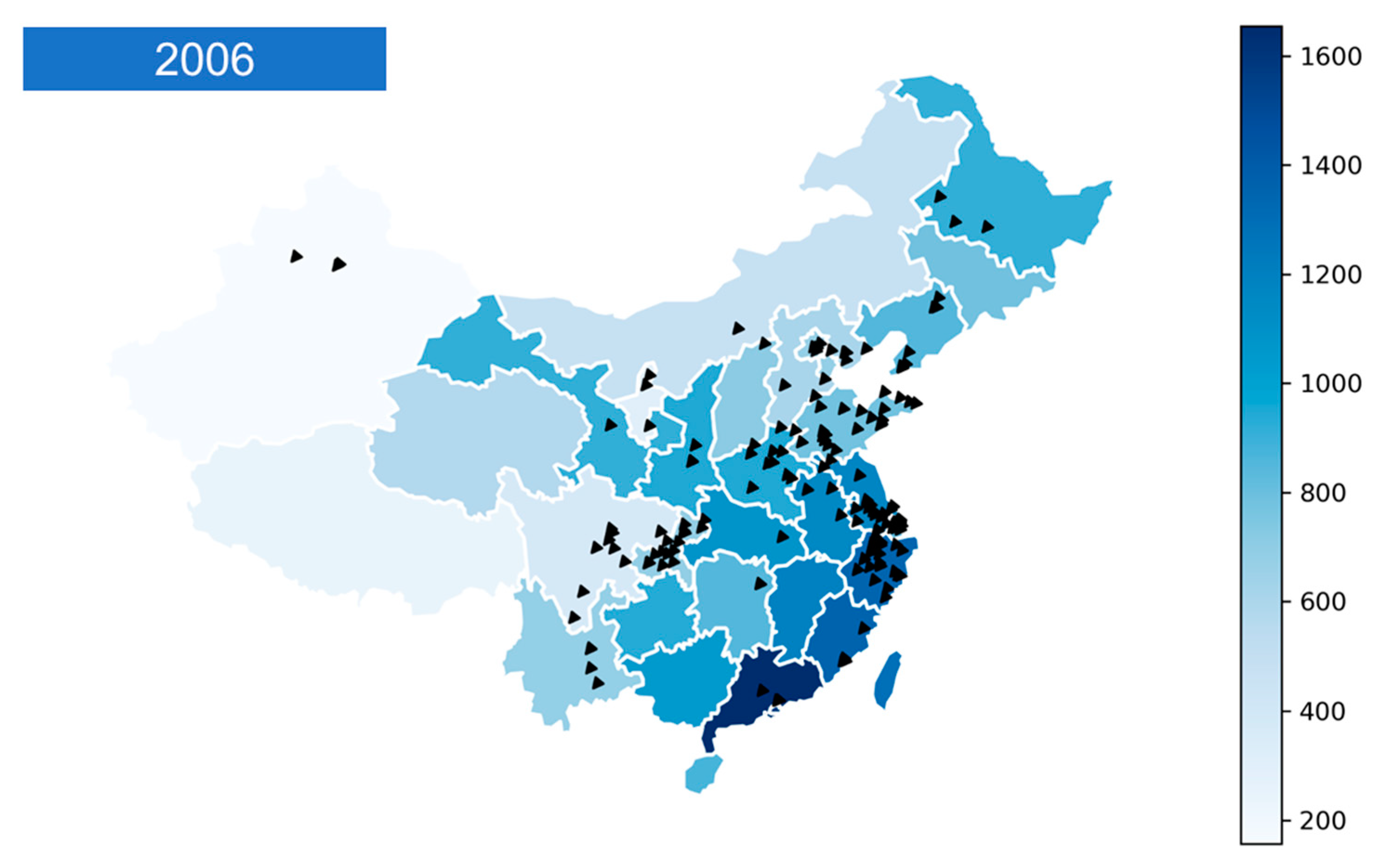
Figure A1.
Annual average temperature levels in sample year (2006), and locations of wastewater treatment plants included in the sample.
Figure A1.
Annual average temperature levels in sample year (2006), and locations of wastewater treatment plants included in the sample.

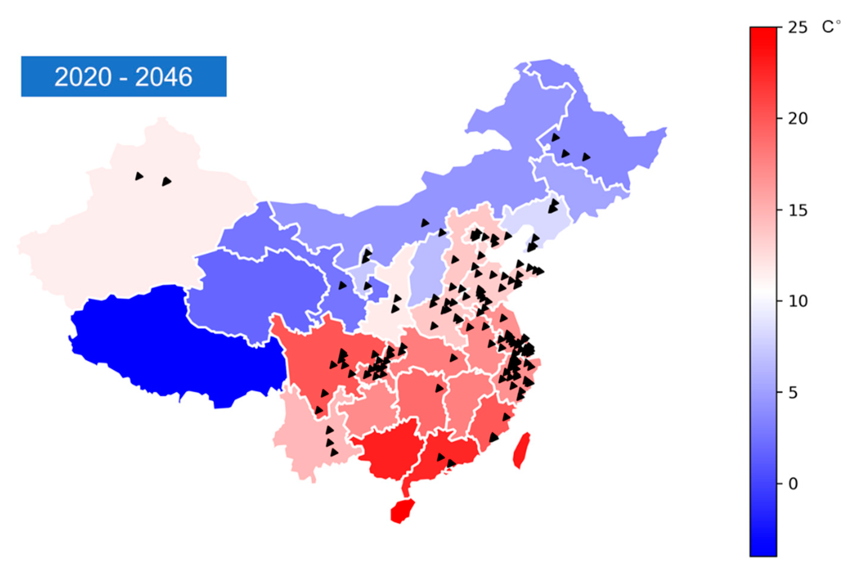
Figure A2.
Annual average temperature levels in short-term future (2020–2046), and locations of wastewater treatment plants included in the sample.
Figure A2.
Annual average temperature levels in short-term future (2020–2046), and locations of wastewater treatment plants included in the sample.

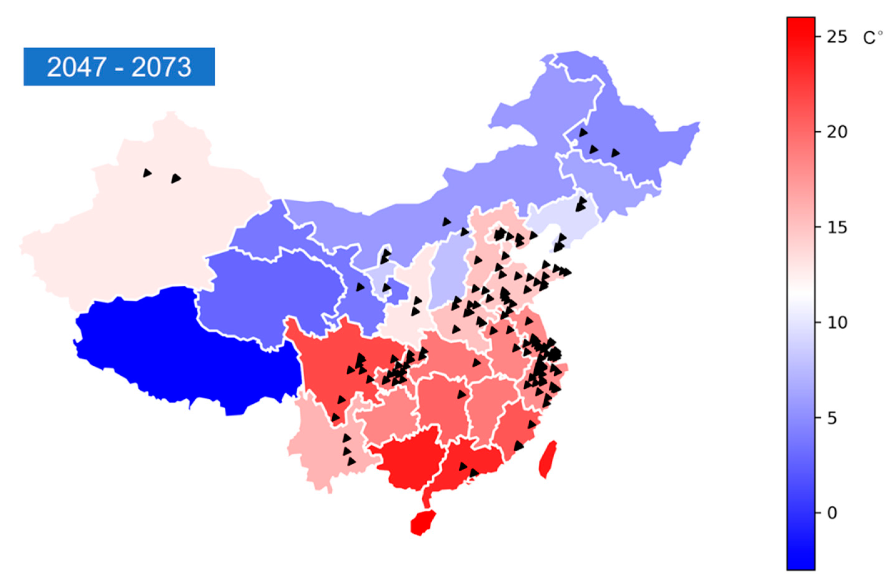
Figure A3.
Annual average temperature levels in mid-term future (2047–2073), and locations of wastewater treatment plants included in the sample.
Figure A3.
Annual average temperature levels in mid-term future (2047–2073), and locations of wastewater treatment plants included in the sample.

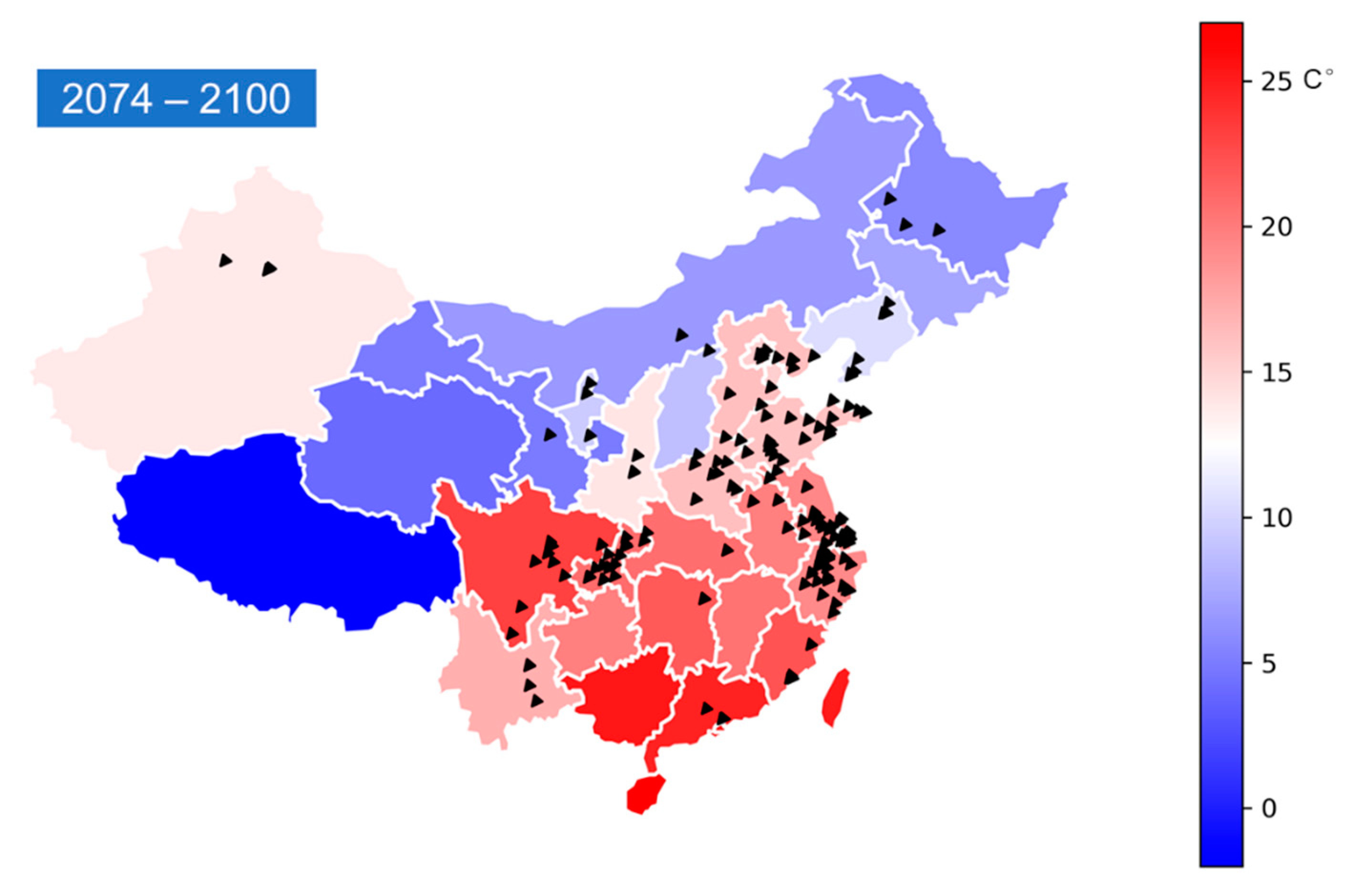
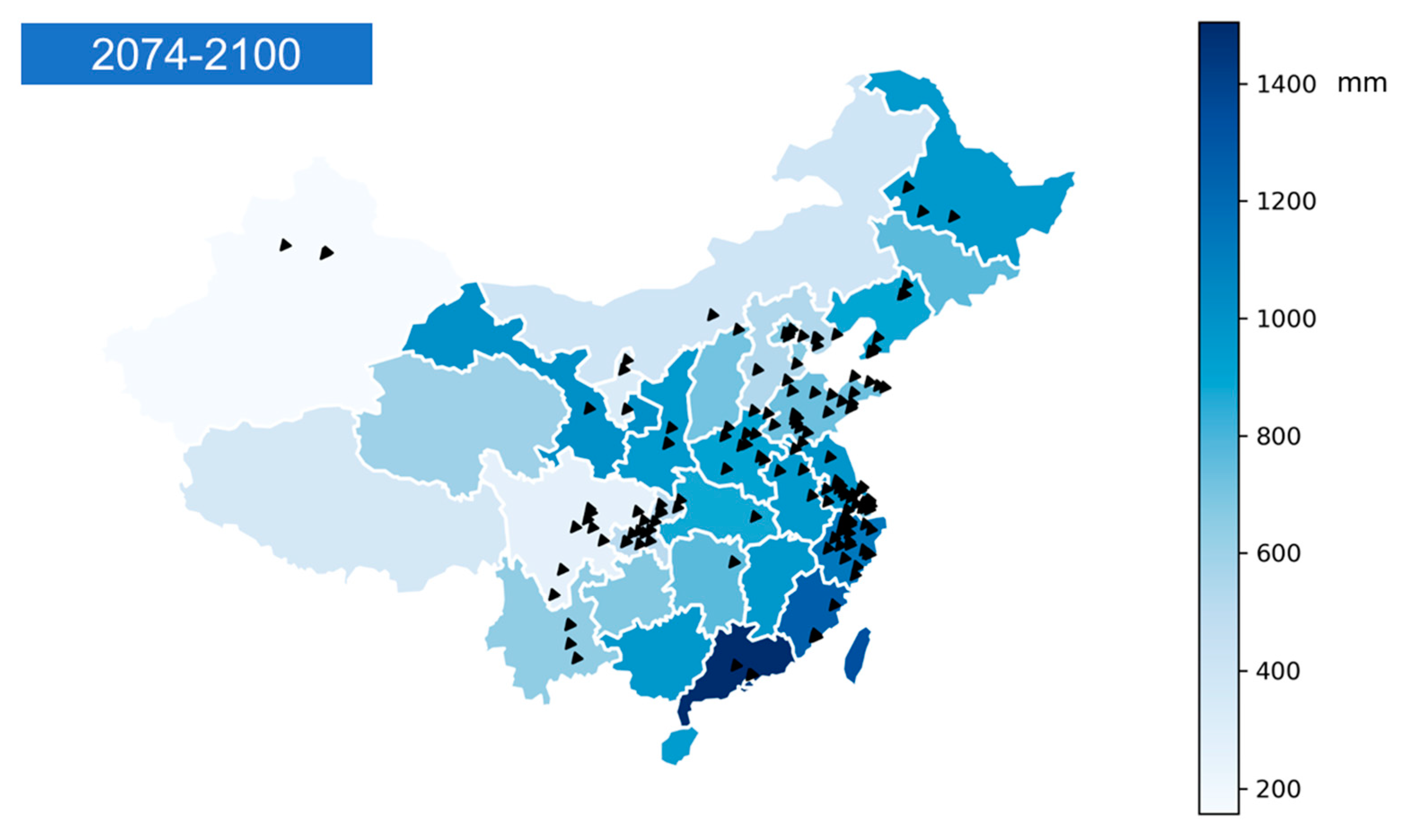
Figure A4.
Annual average temperature levels in long-term future (2074–2100), and locations of wastewater treatment plants included in the sample.
Figure A4.
Annual average temperature levels in long-term future (2074–2100), and locations of wastewater treatment plants included in the sample.

Figure A5.
Annual average precipitation levels in sample year (2006), and locations of wastewater treatment plants included in the sample.
Figure A5.
Annual average precipitation levels in sample year (2006), and locations of wastewater treatment plants included in the sample.

Figure A6.
Annual average precipitation levels in short-term future (2020–2046), and locations of wastewater treatment plants included in the sample.
Figure A6.
Annual average precipitation levels in short-term future (2020–2046), and locations of wastewater treatment plants included in the sample.

Figure A7.
Annual average precipitation levels in mid-term future (2047–2073), and locations of wastewater treatment plants included in the sample.
Figure A7.
Annual average precipitation levels in mid-term future (2047–2073), and locations of wastewater treatment plants included in the sample.

Figure A8.
Annual average precipitation levels in long-term future (2074–2100), and locations of wastewater treatment plants included in the sample.
Figure A8.
Annual average precipitation levels in long-term future (2074–2100), and locations of wastewater treatment plants included in the sample.

References
- Sato, T.; Qadir, M.; Yamamoto, S.; Endo, T.; Zahoor, A. Global, regional, and country level need for data on wastewater generation, treatment, and use. Agric. Water Manag. 2013, 130, 1–13. [Google Scholar] [CrossRef]
- Reznik, A.; Feinerman, E.; Finkelshtain, I.; Fisher, F.; Huber-Lee, A.; Joyce, B.; Kan, I. Economic implications of agricultural reuse of treated wastewater in Israel: A statewide long-term perspective. Ecol. Econ. 2017, 135, 222–233. [Google Scholar] [CrossRef] [Green Version]
- Tol, R.S.J. Estimates of the Damage Costs of Climate Change. Part 1: Benchmark Estimates. Environ. Resour. Econ. 2002, 21, 47–73. [Google Scholar] [CrossRef]
- United Nations Department of Economic and Social Affairs. The Sustainable Development Goals Report. 2018. Available online: https://www.un.org/development/desa/publications/the-sustainable-development-goals-report-2018.html (accessed on 6 August 2018).
- Mideksa, T.K.; Kallbekken, S. The impact of climate change on the electricity market: A review. Energy Policy 2010, 38, 3579–3585. [Google Scholar] [CrossRef]
- Kusangaya, S.; Warburton, M.L.; Van Garderen, E.A.; Jewitt, G.P. Impacts of climate change on water resources in southern Africa: A review. Phys. Chem. Earth Parts A/B/C 2014, 67, 47–54. [Google Scholar] [CrossRef]
- Kurukulasuriya, P.; Mendelsohn, R. Impact and adaptation of South-East Asian farmers to climate change: Conclusions and policy recommendations. Clim. Chang. Econ. 2017, 8, 1740007. [Google Scholar] [CrossRef]
- Jiménez Cisneros, B.E.; Oki, T.; Arnell, N.W.; Benito, G.; Cogley, J.G.; Döll, P.; Jiang, T.; Mwakalila, S.S.; Intergovernmental Panel on Climate Change (IPCC). Climate Change 2014: Impacts, Adaptation, and Vulnerability; Chapter 3, Global and Sectoral Aspects. Contribution of Working Group II to the Fifth Assessment Report of the Intergovernmental Panel on Climate Change; Cambridge University Press: Cambridge, UK; New York, NY, USA, 2014; pp. 229–269. [Google Scholar]
- Schlenker, W.; Roberts, M.J. Nonlinear temperature effects indicate severe damages to U.S. crop yields under climate change. Proc. Natl. Acad. Sci. USA 2009, 106, 15594–15598. [Google Scholar] [CrossRef] [Green Version]
- Kaminski, J.; Kan, I.; Fleischer, A. A Structural Land-Use Analysis of Agricultural Adaptation to Climate Change: A Proactive Approach. Am. J. Agric. Econ. 2013, 95, 70–93. [Google Scholar] [CrossRef]
- Burke, M.; Emerick, K. Adaptation to Climate Change: Evidence from US Agriculture. Am. Econ. Journal: Econ. Policy 2016, 8, 106–140. [Google Scholar] [CrossRef] [Green Version]
- McCarl, B.A.; Thayer, A.W.; Jones, J.P.H. The challenge of climate change adaptation for agriculture: An economically oriented review. J. Agric. Appl. Econ. 2016, 48, 321–344. [Google Scholar] [CrossRef] [Green Version]
- Schlenker, W.; Hanemann, W.M.; Fisher, A.C. Will U.S. Agriculture Really Benefit from Global Warming? Accounting for Irrigation in the Hedonic Approach. Am. Econ. Rev. 2005, 95, 395–406. [Google Scholar] [CrossRef] [Green Version]
- Deschênes, O.; Greenstone, M. The Economic Impacts of Climate Change: Evidence from Agricultural Output and Random Fluctuations in Weather. Am. Econ. Rev. 2007, 97, 354–385. [Google Scholar] [CrossRef] [Green Version]
- Plósz, B.G.; Liltved, H.; Ratnaweera, H. Climate change impacts on activated sludge wastewater treatment: A case study from Norway. Water Sci. Technol. 2009, 60, 533–541. [Google Scholar] [CrossRef]
- U.S. Global Change Research Program. Impacts, Risks, and Adaptation in the United States: The Fourth National Climate Assessment, Volume II; U.S. Global Change Research Program: Washington, DC, USA, 2018; p. 1515. [Google Scholar]
- McMahan, E.K. Impact of rainfall events on wastewater treatment processes. Graduate Theses and Dissertations, University of South Florida, Scholar Commons, Florida, FL, USA, 5 April 2006. [Google Scholar]
- Cromwell, J.E.; Smith, J.B.; Raucher, R.S. Implications of Climate Change for Urban Water Utilities; Association of Metropolitan Water Agencies: Washington, DC, USA, 2007. [Google Scholar]
- Langeveld, J.; Schilperoort, R.; Weijers, S. Climate change and urban wastewater infrastructure: There is more to explore. J. Hydrol. 2013, 476, 112–119. [Google Scholar] [CrossRef]
- Danas, K.; Kurdi, B.; Stark, M.; Mutlaq, A. Climate change effects on waste water treatment. CEE Jordan Group Presentation, Jordan. 18 September 2012. Available online: https://courses.washington.edu/cejordan/CC%20AND%20WWT.pdf (accessed on 18 March 2019).
- Vo, P.T.; Ngo, H.H.; Guo, W.; Zhou, J.L.; Nguyen, P.D.; Listowski, A.; Wang, X.C. A mini-review on the impacts of climate change on wastewater reclamation and reuse. Sci. Total. Environ. 2014, 494, 9–17. [Google Scholar] [CrossRef]
- Zouboulis, A.; Tolkou, A. Effect of Climate Change in Wastewater Treatment Plants: Reviewing the Problems and Solutions. In Managing Water Resources under Climate Uncertainty; Springer Science and Business Media LLC: Cham, Switzerland, 2014; pp. 197–220. [Google Scholar]
- Cromwell, J.; McGuckin, R. Implications of Climate Change for Adaptation by Wastewater and Stormwater Agencies. Proc. Water Environ. Fed. 2010, 2010, 1887–1915. [Google Scholar] [CrossRef]
- Dasgupta, S.; Wheeler, D.; Huq, M.; Zhang, C. Water pollution abatement by Chinese industry: Cost estimates and policy implications. Appl. Econ. 2001, 33, 547–557. [Google Scholar] [CrossRef]
- Chen, H.W.; Chang, N.B. A comparative analysis of methods to represent uncertainty in estimating the cost of constructing wastewater treatment plants. J. Environ. Manag. 2002, 65, 383–409. [Google Scholar] [CrossRef]
- Yu, F.; Niu, K.Y.; Cao, D.; Wang, J.N. Design for a municipal wastewater treatment charge standard system based on cost accounting. China Environ. Sci. 2011, 31, 1578–1584. [Google Scholar]
- Hernández-Sancho, F.; Lamizana-Diallo, B.; Mateo-Sagasta, J.; Qadir, M. Economic valuation of wastewater: The cost of action and the cost of no action. Nairobi: United Nations Environment Programme (UNEP). 2015. Available online: https://wedocs.unep.org/bitstream/handle/20.500.11822/7465/-Economic_Valuation_of_Wastewater_The_Cost_of_Action_and_the_Cost_of_No_Action-2015Wastewater_Evaluation_Report_Mail.pdf.pdf?sequence=3&isAllowed=y (accessed on 6 August 2018).
- Jiang, Y.; Hellegers, P. Joint pollution control in the Lake Tai Basin and the stabilities of the cost allocation schemes. J. Environ. Manag. 2016, 184, 504–516. [Google Scholar] [CrossRef]
- Chai, C.; Zhang, D.; Yu, Y.; Feng, Y.; Wong, M.S. Carbon Footprint Analyses of Mainstream Wastewater Treatment Technologies under Different Sludge Treatment Scenarios in China. Water 2015, 7, 918–938. [Google Scholar] [CrossRef]
- Wang, X.; Wang, X.; Huppes, G.; Heijungs, R.; Ren, N. Environmental implications of increasingly stringent sewage discharge standards in municipal wastewater treatment plants: Case study of a cool area of China. J. Clean. Prod. 2015, 94, 278–283. [Google Scholar] [CrossRef]
- Republic of China State Council. Regulations on Drainage and Sewage Treatment in Towns. 2014; (In Chinese). Available online: http://www.gov.cn/flfg/2013-10/16/content_2508291.htm (accessed on 6 August 2018).
- National Bureau of Statistics of China (NBS). China Statistical Yearbook. 2016. Available online: http://data.stats.gov.cn (accessed on 23 October 2018).
- Ministry of Housing and Urban-Rural Development of China (MOHURD). Statistical Report on Urban and Rural Construction. 2017; (In Chinese). Available online: http://www.mohurd.gov.cn/xytj/tjzljsxytjgb/tjxxtjgb/201708/t20170818_232983.html (accessed on 6 August 2018).
- Ministry of Environmental Protection of the People’s Republic of China (MOEP). Environmental Statistics Bulletin. 2014. Available online: http://www.mep.gov.cn/ (accessed on 6 August 2018).
- Jin, L.; Zhang, G.; Tian, H. Current state of sewage treatment in China. Water Res. 2014, 66, 85–98. [Google Scholar] [CrossRef] [PubMed]
- Zhang, Q.; Yang, W.; Ngo, H.H.; Guo, W.; Jin, P.; Dzakpasu, M.; Yang, S.; Wang, Q.; Wang, X.; Ao, D. Current status of urban wastewater treatment plants in China. Environ. Int. 2016, 92, 11–22. [Google Scholar] [CrossRef]
- Ministry of Environmental Protection of the People’s Republic of China (MOEP). Discharge Standard of Pollutants for Municipal Wastewater Treatment Plant GB18918-2002. 2002. Available online: https://www.ecolex.org/details/legislation/discharge-standard-of-pollutants-for-municipal-wastewater-treatment-plant-national-standard-gb-18918-2002-lex-faoc136765/ (accessed on 6 August 2018).
- Sun, Y.; Chen, Z.; Wu, G.; Wu, Q.; Zhangbin, N.; Niu, Z.; Hu, H.-Y. Characteristics of water quality of municipal wastewater treatment plants in China: Implications for resources utilization and management. J. Clean. Prod. 2016, 131, 1–9. [Google Scholar] [CrossRef] [Green Version]
- Jiang, Y.; Dinar, A.; Hellegers, P. Economics of social trade-off: Balancing wastewater treatment cost and ecosystem damage. J. Environ. Manag. 2018, 211, 42–52. [Google Scholar] [CrossRef]
- Tchobanoglous, G.; Burton, F.L. Wastewater Engineering: Treatment, Disposal and Reuse; McGraw-Hill: New York, NY, USA, 1991. [Google Scholar]
- Harris, I.R.; Jones, P.D.; Osborn, T.; Lister, D.H. Updated high-resolution grids of monthly climatic observations—The CRU TS3.10 Dataset. Int. J. Clim. 2014, 34, 623–642. [Google Scholar] [CrossRef] [Green Version]
- Piao, S.; Ciais, P.; Huang, Y.; Shen, Z.; Peng, S.; Li, J.; Zhou, L.; Liu, H.; Ma, Y.; Ding, Y.; et al. The impacts of climate change on water resources and agriculture in China. Nature 2010, 467, 43–51. [Google Scholar] [CrossRef]
- Fraas, A.G.; Munley, V.G. Municipal wastewater treatment cost. J. Environ. Econ. Manag. 1984, 11, 28–38. [Google Scholar] [CrossRef]
- Schwarz, G.E.; McConnell, V.D. Local choice and wastewater treatment plant performance. Water Resour. Res. 1993, 29, 1589–1600. [Google Scholar] [CrossRef]
- Fraquelli, G.; Giandrone, R. Reforming the wastewater treatment sector in Italy: Implications of plant size, structure, and scale economies. Water Resour. Res. 2003, 39, 1293. [Google Scholar] [CrossRef]
- Friedler, E.; Pisanty, E. Effects of design flow and treatment level on construction and operation costs of municipal wastewater treatment plants and their implications on policy making. Water Res. 2006, 40, 3751–3758. [Google Scholar] [CrossRef] [PubMed]
- Hernández-Sancho, F.; Molinos-Senante, M.; Sala-Garrido, R. Cost modelling for wastewater treatment processes. Desalination 2011, 268, 1–5. [Google Scholar] [CrossRef]
- Sala-Garrido, R.; Molinos-Senante, M.; Hernández-Sancho, F. Comparing the efficiency of wastewater treatment technologies through a DEA metafrontier model. Chem. Eng. J. 2011, 173, 766–772. [Google Scholar] [CrossRef]
- Molinos-Senante, M.; Hernandezsancho, F.; Sala-Garrido, R. Comparing the dynamic performance of wastewater treatment systems: A metafrontier Malmquist productivity index approach. J. Environ. Manag. 2015, 161, 309–316. [Google Scholar] [CrossRef]
- Molinos-Senante, M.; Sala-Garrido, R.; Lafuente, M. The role of environmental variables on the efficiency of water and sewerage companies: A case study of Chile. Environ. Sci. Pollut. Res. 2015, 22, 10242–10253. [Google Scholar] [CrossRef]
- Sato, N.; Okubo, T.; Onodera, T.; Agrawal, L.K.; Ohashi, A.; Harada, H. Economic evaluation of sewage treatment processes in India. J. Environ. Manag. 2007, 84, 447–460. [Google Scholar] [CrossRef]
- Niu, K.; Wu, J.; Yu, F.; Guo, J. Construction and Operation Costs of Wastewater Treatment and Implications for the Paper Industry in China. Environ. Sci. Technol. 2016, 50, 12339–12347. [Google Scholar] [CrossRef]
- Tran, Q.K.; Schwabe, K.A.; Jassby, D. Wastewater Reuse for Agriculture: Development of a Regional Water Reuse Decision-Support Model (RWRM) for Cost-Effective Irrigation Sources. Environ. Sci. Technol. 2016, 50, 9390–9399. [Google Scholar] [CrossRef]
- Tran, Q.; Jassby, D.; Schwabe, K.A. The implications of drought and water conservation on the reuse of municipal wastewater: Recognizing impacts and identifying mitigation possibilities. Water Res. 2017, 124, 472–481. [Google Scholar] [CrossRef]
- Lin, G.; Fu, J.; Jiang, D.; Wang, J.; Wang, Q.; Dong, D. Spatial Variation of the Relationship between PM2.5 Concentrations and Meteorological Parameters in China. BioMed Res. Int. 2015, 2015, 1–15. [Google Scholar] [CrossRef] [PubMed]
- Ramsey, J.B. Tests for Specification Errors in Classical Linear Least-Squares Regression Analysis. J. R. Stat. Soc. Ser. Stat. Methodol. 1969, 31, 350–371. [Google Scholar] [CrossRef]
- Zhou, Y.; Duan, N.; Wu, X.; Fang, H. COD Discharge Limits for Urban Wastewater Treatment Plants in China Based on Statistical Methods. Water 2018, 10, 777. [Google Scholar] [CrossRef] [Green Version]
- Lavee, D. Is the upgrading of wastewater treatment facilities to meet more stringent standards economically justified: The case of Israel. Water Resour. 2014, 41, 564–573. [Google Scholar] [CrossRef]
- Wang, R. Environmental and resource sustainability of Chinese cities: A review of issues, policies, practices and effects. Nat. Resour. Forum 2011, 35, 112–121. [Google Scholar] [CrossRef]
- Taylor, K.E.; Stouffer, R.J.; Meehl, G.A. An Overview of CMIP5 and the Experiment Design. Bull. Am. Meteorol. Soc. 2012, 93, 485–498. [Google Scholar] [CrossRef] [Green Version]
- Wang, J.; Mendelsohn, R.; Dinar, A.; Huang, J.; Rozelle, S.; Zhang, L. The impact of climate change on China’s agriculture. Agric. Econ. 2009, 40, 323–337. [Google Scholar] [CrossRef]
- Xu, C.H.; Xu, Y. The projection of temperature and precipitation over China under RCP scenarios using a CMIP5 multi-model ensemble. Atmos. Oceanic Sci. Lett. 2012, 5, 527–533. [Google Scholar]
- Hui, P.; Tang, J.; Wang, S.; Wang, S.; Zong, P.; Dong, X. Climate change projections over China using regional climate models forced by two CMIP5 global models. Part II: Projections of future climate. Int. J. Clim. 2018, 38, e78–e94. [Google Scholar] [CrossRef]
- Bao, Q.; Lin, P.; Zhou, T.; Liu, Y.; Yu, Y.; Wu, G.; He, B.; He, J.; Li, L.; Li, J.; et al. The Flexible Global Ocean-Atmosphere-Land system model, Spectral Version 2: FGOALS-s2. Adv. Atmos. Sci. 2013, 30, 561–576. [Google Scholar] [CrossRef]
- Zhang, Y.; You, Q.; Chen, C.; Ge, J. Impacts of climate change on streamflows under RCP scenarios: A case study in Xin River Basin, China. Atmos. Res. 2016, 178, 521–534. [Google Scholar] [CrossRef]
- Shalizi, Z. Water and urbanization. In China Urbanizes: Consequences, Strategies and Policies; Yusuf, S., Saich, T., Eds.; World Bank: Washington, DC, USA, 2008. [Google Scholar]
- Wang, X.-J.; Zhang, J.-Y.; Shahid, S.; Xie, W.; Du, C.-Y.; Shang, X.-C.; Zhang, X. Modeling domestic water demand in Huaihe River Basin of China under climate change and population dynamics. Environ. Dev. Sustain. 2017, 20, 911–924. [Google Scholar] [CrossRef]
- United Nations (UN) Department of Economic and Social Affairs (DESA), Population Division. World Population Prospects. 2017. Available online: https://population.un.org/wpp/Download/Standard/Population/ (accessed on 6 August 2018).
- European Union Small and Medium-Sized Enterprise (EUSME) Centre. The Water Sector in China. 2013. Available online: http://www.eusmecentre.org.cn/report/water-sector-china (accessed on 15 November 2018).
- Nordhaus, W.D. A Review of the Stern Review on the Economics of Climate Change. J. Econ. Lit. 2007, 45, 686–702. [Google Scholar] [CrossRef]
- Feinerman, E.; Plessner, Y.; Eshel, D.M.D. Recycled Effluent: Should the Polluter Pay? Am. J. Agric. Econ. 2001, 83, 958–971. [Google Scholar] [CrossRef]
- McConnell, V.D.; Schwarz, G.E. The supply and demand for pollution control: Evidence from wastewater treatment. J. Environ. Econ. Manag. 1992, 23, 54–77. [Google Scholar] [CrossRef]
- Fernandez, L. Estimation of Wastewater Treatment Objectives through Maximum Entropy. J. Environ. Econ. Manag. 1997, 32, 293–308. [Google Scholar] [CrossRef]
- Hernández-Sancho, F.; Sala-Garrido, R. Technical efficiency and cost analysis in wastewater treatment processes: A DEA approach. Desalination 2009, 249, 230–234. [Google Scholar] [CrossRef]
- Hernandezsancho, F.; Molinossenante, M.; Sala-Garrido, R. Energy efficiency in Spanish wastewater treatment plants: A non-radial DEA approach. Sci. Total. Environ. 2011, 409, 2693–2699. [Google Scholar] [CrossRef]
Figure 1.
Relationship between historical climate variables in the dataset. (a) Annual average temperature and precipitation levels for each wastewater treatment plant in the sample; (b) Annual average temperature levels and intra-annual variation in temperature for each wastewater treatment plant in the sample; (c) Annual average precipitation levels and intra-annual variation in precipitation for each wastewater treatment plant in the sample.

Figure 2.
Temporal variation in climate (temperature) variables in the sample. (a) Ratio between observed and historical annual average temperature levels for each wastewater treatment plant with respect to historical annual average temperature levels; (b) Ratio between observed and historical intra-annual variation in temperature for each wastewater treatment plant with respect to historical intra-annual variation in temperature.

Figure 3.
Temporal variation in climate (precipitation) variables in the sample. (a) Ratio between observed and historical annual average precipitation levels for each wastewater treatment plant with respect to historical annual average precipitation levels; (b) Ratio between observed and historical intra-annual variation in precipitation for each wastewater treatment plant with respect to historical intra-annual variation in precipitation.

Figure 4.
Future trajectories of wastewater flows (index, 2020 = 100). Labels V1 through V6 refer to different trends of predicted wastewater flows.
Figure 4.
Future trajectories of wastewater flows (index, 2020 = 100). Labels V1 through V6 refer to different trends of predicted wastewater flows.

Table 1.
Descriptive statistics of the cost model variables.
| Variable | Units | Mean | Std. Dev. | Min | Max |
|---|---|---|---|---|---|
| Dependent Variable | |||||
| O&M Costs | Million $ | 1.95 | 1.46 | 0.15 | 8.24 |
| Explanatory Variables | |||||
| Investment | Million $ | 28.75 | 26.37 | 1.86 | 139.41 |
| Volume Treated | 104 × m3/day | 6.46 | 6.32 | 0.21 | 40.00 |
| Treatment Capacity | 104 × m3/day | 7.54 | 7.04 | 0.60 | 40.00 |
| Tenure (years since establishment) | Years | 8.77 | 6.47 | 1.00 | 50.00 |
| BOD Influent | mg/L | 169.99 | 89.00 | 17.99 | 480.00 |
| BOD Effluent | mg/L | 13.40 | 8.34 | 1.20 | 60.00 |
Notes: Acronym BOD stands for biological oxygen demand.
Table 2.
Shares of treatment processes by number of treatment plants, and total designed capacity in the sample and the entire sector, (percent).
Table 2.
Shares of treatment processes by number of treatment plants, and total designed capacity in the sample and the entire sector, (percent).
| Treatment Process | Number of WWTPs | Designed Capacity | ||||
|---|---|---|---|---|---|---|
| Sample (2006) | Reported in [35] | Reported in [36] | Sample (2006) | Reported in [35] | Reported in [36] | |
| AAO | 12 | 25 | 31 | 17 | 33 | 21 |
| Chemical and Physicochemical | 3 | 1 | 3 | 3 | 2 | 3 |
| AO | 6 | 6 | 8 | 4 | 8 | 5 |
| Biological Film | 3 | 2 | 4 | 2 | 1 | 6 |
| AS | 15 | 9 | 11 | 21 | 4 | 15 |
| SBR | 10 | 17 | 10 | 8 | 10 | 11 |
| Oxidation Ditch | 40 | 29 | 21 | 35 | 28 | 25 |
| Others | 11 | 11 | 12 | 10 | 14 | 14 |
Notes: Initials AAO stands for Anaerobic/Anoxic/Oxic. Initials AO stands for Anoxic-Oxic. Initals AS stands for Activated Sludge. Initials SBR stands for Sequencing Batch Reactors.
Table 3.
Descriptive statistics of climate variables.
| Historical Climate | Observed Weather | ||||
|---|---|---|---|---|---|
| Units | Mean | Std. Dev. | Mean | Std. Dev. | |
| Temperature | |||||
| Annual Average | C° | 14.28 | 3.41 | 15.31 | 3.40 |
| Intra Annual Variance | (C°)2 | 87.67 | 36.54 | 85.89 | 35.76 |
| Precipitation | |||||
| Annual Average | mm | 975.78 | 387.05 | 901.32 | 426.39 |
| Intra Annual Variance | (mm)2 | 5390.59 | 3746.01 | 4337.57 | 3880.45 |
Table 4.
Estimated coefficients for O&M cost equation under different specifications.
| Variable\Model | A | B | C | D |
|---|---|---|---|---|
| Investment () | 0.267 (0.068) | 0.159 (0.070) | 0.290 (0.070) | 0.182 (0.072) |
| Capacity () | 0.566 (0.166) | 0.714 (0.166) | 0.493 (0.173) | 0.657 (0.170) |
| Volume () | −0.095 (0.149) | −0.127 (0.144) | −0.076 (0.150) | −0.115 (0.145) |
| Tenure () | 0.079 (0.084) | 0.040 (0.126) | 0.301 (0.149) | 0.221 (0.171) |
| Quality Parameters | ||||
| BOD Influent () | 0.167 (0.077) | 0.168 (0.079) | 0.168 (0.079) | 0.171 (0.080) |
| BOD Effluent () | −0.030 (0.063) | −0.036 (0.065) | −0.03 (0.063) | −0.036 (0.065) |
| Climate Indicators | ||||
| Hist. Mean Temp. () | 0.091 (0.224) | 0.395 (0.450) | 0.061 (0.224) | 0.451 (0.450) |
| Hist. Intra-Ann. Temp. Var. () | 0.376 (0.135) | 0.054 (0.439) | 0.366 (0.135) | 0.306 (0.465) |
| Mean Temp. Ratio () | −0.753 (1.445) | 0.538 (3.678) | −0.881 (1.455) | −0.497 (4.094) |
| Intra-Ann. Temp Var. Ratio () | 2.190 (0.817) | 3.167 (2.756) | 2.423 (0.836) | 2.052 (2.885) |
| Treatment Technologies () | ||||
| Chemical and Physicochemical | −0.349 (0.148) | −0.247 (0.174) | −0.362 (0.149) | −0.235 (0.176) |
| AAO | −0.156 (0.148) | 0.012 (0.160) | −0.175 (0.153) | −0.001 (0.161) |
| AO | −0.314 (0.191) | −0.047 (0.195) | −0.353 (0.192) | −0.077 (0.195) |
| Biological Filter | −0.278 (0.240) | −0.208 (0.261) | −0.304 (0.242) | −0.209 (0.262) |
| SBR | 0.021 (0.160) | 0.073 (0.173) | 0.016 (0.163) | 0.073 (0.173) |
| Oxidation Ditch | −0.122 (0.118) | 0.032 (0.132) | −0.137 (0.125) | 0.024 (0.139) |
| Not Specified | −1.292 (0.363) | −1.301 (0.357) | −1.352 (0.370) | −1.290 (0.366) |
| Constant Term | −3.778 (1.099) | −2.453 (2.779) | −4.827 (1.332) | −4.412 (3.107) |
| Control Vectors | ||||
| Province () | No | Yes | No | Yes |
| Decade () | No | No | Yes | Yes |
| Adjusted R2 | 0.659 | 0.714 | 0.660 | 0.718 |
| Moran I | 1.710 | 0.310 | 2.960 | 1.070 |
Notes: Standard errors are reported in parenthesis. The coefficients presented under column 3 (C) are based on a maximum likelihood estimation of a spatial autoregressive procedure.
Table 5.
Temperature predictions by climate model, emission scenario and future period.
| Variable | Annual Average (C°) | Intra-Annual Variance (C°)2 | ||||
|---|---|---|---|---|---|---|
| Period and Model | RCP 2.6 | RCP 4.5 | RCP 8.5 | RCP 2.6 | RCP 4.5 | RCP 8.5 |
| Base (2006) | 14.32 | 87.25 | ||||
| BCC-CSM1 | 14.53 | 14.61 | 14.92 | 88.54 | 92.44 | 87.52 |
| CanESM2 | 16.14 | 16.11 | 16.36 | 86.01 | 87.27 | 85.49 |
| GISS-E2-R | 15.22 | 15.37 | 15.69 | 60.83 | 60.95 | 58.61 |
| MIROC5 | 16.35 | 16.37 | 16.61 | 95.39 | 96.27 | 95.31 |
| MIROC-ESM | 16.33 | 16.13 | 16.51 | 90.15 | 91.56 | 90.67 |
| MIROC-ESM-CHEM | 16.47 | 16.03 | 16.55 | 94.07 | 94.23 | 92.96 |
| MPI-ESM-LR | 15.19 | 15.24 | 15.35 | 78.48 | 80.12 | 81.63 |
| Average (2020-2046) | 15.75 | 15.69 | 16.00 | 84.78 | 86.12 | 84.60 |
| BCC-CSM1 | 14.77 | 15.18 | 16.10 | 90.35 | 89.96 | 90.20 |
| CanESM2 | 16.42 | 16.92 | 17.85 | 85.39 | 88.11 | 88.27 |
| GISS-E2-R | 15.17 | 15.83 | 16.62 | 59.47 | 59.43 | 59.21 |
| MIROC5 | 17.09 | 17.43 | 18.27 | 97.17 | 95.26 | 95.49 |
| MIROC-ESM | 16.72 | 17.45 | 18.55 | 93.60 | 93.27 | 91.79 |
| MIROC-ESM-CHEM | 16.72 | 17.21 | 18.42 | 92.25 | 95.18 | 91.24 |
| MPI-ESM-LR | 15.16 | 15.69 | 16.84 | 78.77 | 79.91 | 76.92 |
| Average (2047–2073) | 16.01 | 16.53 | 17.52 | 85.29 | 85.87 | 84.73 |
| BCC-CSM1 | 14.63 | 15.44 | 17.57 | 91.31 | 89.68 | 93.77 |
| CanESM2 | 16.29 | 17.37 | 19.56 | 87.49 | 86.78 | 91.73 |
| GISS-E2-R | 14.92 | 15.82 | 17.73 | 60.06 | 62.03 | 57.37 |
| MIROC5 | 17.15 | 17.89 | 19.66 | 96.45 | 97.03 | 95.31 |
| MIROC-ESM | 16.85 | 17.80 | 20.78 | 94.83 | 94.73 | 90.92 |
| MIROC-ESM-CHEM | 16.62 | 17.69 | 20.74 | 97.04 | 94.32 | 91.25 |
| MPI-ESM-LR | 14.98 | 16.04 | 18.38 | 78.65 | 77.38 | 77.71 |
| Average (2074–2100) | 15.92 | 16.86 | 19.20 | 86.55 | 85.99 | 85.44 |
Observed and predicted annual average temperature and precipitation levels across China, as well as the locations of wastewater treatment plants included in the sample are presented in Appendix B.
Table 6.
Simulated future climate change impacts on wastewater treatment costs.
| Variables | Annual O&M Costs (Million $) | Per Unit of Wastewater Treated O&M Cost ($/m3) | |||||||
|---|---|---|---|---|---|---|---|---|---|
| Entire Sample (θS) | Average Plant (θP) | Average Plant (μP) | |||||||
| R1 | R2 | R3 | R1 | R2 | R3 | R1 | R2 | R3 | |
| Base | 302.031 | 1.853 | 0.106 | ||||||
| G1 | 329.362 | 358.274 | 339.455 | 2.021 | 2.198 | 2.083 | 0.143 | 0.155 | 0.147 |
| G2 | 281.974 | 300.643 | 305.689 | 1.730 | 1.844 | 1.875 | 0.128 | 0.137 | 0.141 |
| G3 | 81.056 | 82.476 | 75.737 | 0.497 | 0.506 | 0.465 | 0.029 | 0.030 | 0.027 |
| G4 | 349.028 | 350.360 | 351.665 | 2.141 | 2.149 | 2.157 | 0.127 | 0.128 | 0.129 |
| G5 | 313.543 | 323.116 | 315.857 | 1.924 | 1.982 | 1.938 | 0.133 | 0.137 | 0.131 |
| G6 | 333.101 | 339.844 | 327.530 | 2.044 | 2.085 | 2.009 | 0.135 | 0.138 | 0.132 |
| G7 | 176.581 | 186.171 | 194.034 | 1.083 | 1.142 | 1.190 | 0.069 | 0.072 | 0.076 |
For brevity purposes, we only present results from high- and low-discount rate computations in a summary form. We refer the interested reader to the Supplementary Materials attached to this paper for the detailed reports.
Table 7.
Differences in calculated cost measures between scenarios.
| Variables | Annual O&M Costs (Million $) | Per Unit of Wastewater Treated O&M Cost ($/m3) | |||||
|---|---|---|---|---|---|---|---|
| Entire Sample (θS) | Average Plant (θP) | Cheapest Plant | Most Expensive Plant | Average Plant (μP) | Cheapest Plant | Most Expensive Plant | |
| Sim2–Sim3 | 36.999 | 0.227 | 0.025 | 1.287 | 0.015 | 0.002 | 0.057 |
| Sim1–Sim3 | 80.032 | 0.491 | −0.006 | 4.585 | 0.044 | −0.003 | 1.336 |
| Ratio (percent) | 46 | 46 | −407 | 28 | 33 | −94 | 4 |
Notes: Figures in the tables are rounded to the third decimal, whereas the ratios presented are based on the actual numbers.
Table 8.
Ratio of differences in calculated annual O&M costs between simulations by climate models and emission scenarios.
Table 8.
Ratio of differences in calculated annual O&M costs between simulations by climate models and emission scenarios.
| Variable | Annual O&M Costs for an Average Plant (θP) | Per Unit of Wastewater Treated O&M Costs in an Average Plant (μP) | ||||
|---|---|---|---|---|---|---|
| GCM/RCP | R1 | R2 | R3 | R1 | R2 | R3 |
| G1 | 27 | 23 | 26 | 19 | 17 | 19 |
| G2 | 41 | 34 | 33 | 25 | 21 | 20 |
| G3 | -35 | −36 | −34 | −41 | −41 | -39 |
| G4 | 24 | 24 | 24 | 25 | 24 | 24 |
| G5 | 31 | 29 | 30 | 22 | 21 | 23 |
| G6 | 27 | 25 | 28 | 22 | 21 | 23 |
| G7 | −306 | −1496 | 840 | 665 | 266 | 165 |
Table 9.
Ratio of differences in calculated annual operating and maintenance costs between simulations by volume and policy scenarios.
Table 9.
Ratio of differences in calculated annual operating and maintenance costs between simulations by volume and policy scenarios.
| Variable | Annual O&M Costs for an Average Plant (θP) | Per Unit of Wastewater Treated O&M Costs in an Average Plant (μP) | ||||||
|---|---|---|---|---|---|---|---|---|
| Wastewater Volume/Policy Scenario | P0 | P1 | P2 | P3 | P0 | P1 | P2 | P3 |
| V0 | −30 | −21 | −27 | −29 | 54 | 56 | 54 | 54 |
| V1 | 29 | 37 | 33 | 30 | 107 | 122 | 110 | 108 |
| V2 | −7 | −1 | −5 | −6 | 63 | 66 | 64 | 63 |
| V3 | −28 | −20 | −26 | −28 | 55 | 57 | 56 | 56 |
| V4 | −55 | −43 | −51 | −53 | 50 | 51 | 50 | 50 |
| V5 | −23 | −16 | −21 | −23 | 52 | 53 | 52 | 52 |
| V6 | −128 | −98 | −120 | −125 | 45 | 46 | 45 | 45 |
Publisher’s Note: MDPI stays neutral with regard to jurisdictional claims in published maps and institutional affiliations. |
© 2020 by the authors. Licensee MDPI, Basel, Switzerland. This article is an open access article distributed under the terms and conditions of the Creative Commons Attribution (CC BY) license (http://creativecommons.org/licenses/by/4.0/).
Share and Cite
MDPI and ACS Style
Reznik, A.; Jiang, Y.; Dinar, A. The Impacts of Climate Change on Wastewater Treatment Costs: Evidence from the Wastewater Sector in China. Water 2020, 12, 3272. https://doi.org/10.3390/w12113272
AMA Style
Reznik A, Jiang Y, Dinar A. The Impacts of Climate Change on Wastewater Treatment Costs: Evidence from the Wastewater Sector in China. Water. 2020; 12(11):3272. https://doi.org/10.3390/w12113272
Chicago/Turabian StyleReznik, Ami, Yu Jiang, and Ariel Dinar. 2020. "The Impacts of Climate Change on Wastewater Treatment Costs: Evidence from the Wastewater Sector in China" Water 12, no. 11: 3272. https://doi.org/10.3390/w12113272
Note that from the first issue of 2016, this journal uses article numbers instead of page numbers. See further details here.