Airborne Radiometry for Calibration, Validation, and Research in Oceanic, Coastal, and Inland Waters

Introduction

The lack of optimized remote sensing capabilities for coastal and inland waters that can bridge limited spatial coverage and high temporal resolution observations from in-water systems, such as buoys, as well as limited spatial and temporal coverage of ship-based validation with the coarse spatial, temporal, and spectral resolution of satellite data for ocean color products is a significant gap. In contrast to the open ocean, coastal and inland waters are difficult regions to accurately retrieve ocean color radiant flux (Dierssen et al., 2006; Dunagan et al., 2009; Guild et al., 2011, 2019; Turpie et al., 2015, 2016). In coastal areas, the magnitude of the radiance signal in the visible (VIS) range (400–700 nm) is highly variable, ranging from very dark values in clear, deep water, as well as in water dominated by colored dissolved organic matter (CDOM) (e.g., Brezonik et al., 2015; Palmer et al., 2015). For example, typical albedo for deep ocean water is often assumed to be approximately 5% (Moses et al., 2012), but productive and turbid inland waters can easily exceed 25% or more (Kudela et al., 2019). Legacy and presently operational ocean color satellite sensors such as Sea-viewing Wide Field-of-View Sensor (SeaWiFS), Moderate Resolution Imaging Spectrometer (MODIS), Medium Resolution Imaging Spectrometer (MERIS), and the Visible Infrared Imaging Radiometer Suite (VIIRS) are optimally designed for open-ocean imagery. They are calibrated for low spectral water-leaving radiances, L_W(λ), and produce coarse spatial (km) and spectral resolution. While more recent sensors, such as the Ocean Land Color Instrument (OLCI), Operational Land Imager (OLI), and Multispectral Instrument (MSI), provide improved spatial and spectral resolution, they are not optimized for retrievals over inland waters (Kudela et al., 2019).

Radiance signals are also highly variable in space and time at the land–sea interface due to the dynamic nature of this region. Low signal-to-noise ratio (SNR) measurements of L_W(λ) in the blue spectral domain result in negative values using standard re-processing, leading to poor discrimination of pigments from CDOM and poor estimates in the ultraviolet (UV). Aerosol and trace gas plumes from continental sources complicate the task of atmospheric correction, as does cloud cover. Aerosols and water vapor strongly scatter and absorb light in the same region of the spectrum where some ocean color algorithms are derived (e.g., chlorophyll), compounding the problems associated with atmospheric correction and low SNR. Atmospheric correction schemes are also problematic for productive coastal waters. Issues include the use of non-zero near-infrared (NIR) radiances and poor SNR values, complicating the use of short-wave infrared (SWIR) observations to improve atmospheric correction (Siegel et al., 2000; Shi and Wang, 2009; Werdell et al., 2010). The UV is also potentially useful for discriminating red tides (Kahru and Mitchell, 1998), identifying point sources for pollution (Hooker et al., 2013), and improving atmospheric correction, particularly in turbid coastal waters (Wang et al., 2007; Gao et al., 2009; He et al., 2012). Frequent atmospheric correction failures occur at moderate to high chlorophyll levels, leading to data loss in these dynamic regions (Loisel et al., 2013; Houskeeper and Kudela, 2019), while most existing instruments for calibration, validation, and research (CVR) measurements, as well as spectral radiometers, exhibit poor performance in the UV.

The limited legacy and presently operational ocean color satellites (Groom et al., 2019) having both multiple mid-range spectral bands (500–600 nm) and high spatial resolution spaceborne sensors makes it difficult to detect high biomass events and “red tides” (Dierssen et al., 2006), one of the main targets for coastal and inland water remote sensing. While this can be mitigated to some extent by switching to red or infrared bands (Houskeeper and Kudela, 2019), there can be both over- and under-estimates based on the specific band configuration (Ryan et al., 2014). There is a demonstrable need for high spatial, spectral, and temporal resolution data to meet these challenges. For the foreseeable future, this can be enhanced with airborne instrumentation well suited for smaller water bodies and enabling higher spatial and spectral resolution measurements (Davis et al., 2007; Gholizadeh et al., 2016) and with agility in timing for event response and time of day for science needs. To bridge the gap between open ocean, coastal, and inland waters, innovation and selection of relevant aquatic airborne instruments for CVR and flight planning to support the science and instrument requirements is crucial (Guild et al., 2011, 2019). Further, aligned sensor technology, site coverage, and data collection contemporaneous with in-water observations enable credible CVR in dynamic coastal and inland aquatic environments. To meet these observational and innovative technology needs, next-generation instrument suites, processing, and data products have been tested in coastal and inland waters during several recent airborne missions on the Naval Postgraduate School’s (NPS) Twin Otter (TO): (a) 2011 NASA Coastal and Ocean Airborne Science Testbed (COAST); (b) 2013 NASA Ocean Color Ecosystem Assessments using Novel Instruments and Aircraft (OCEANIA); and (c) the 2017 and 2018 Coastal High Acquisition Rate Radiometers for Innovative Environmental Research (C-HARRIER) campaigns (Table 1). These airborne mission technology developments advanced from establishing the flight observation requirements for the instruments individually or as a sensor suite, to flight scenarios that address the remote sensing needs of aquatic environments in support of satellite observations (or high-altitude simulations thereof), and including the processing of airborne data for aquatic CVR for ocean, coastal, and inland targets.

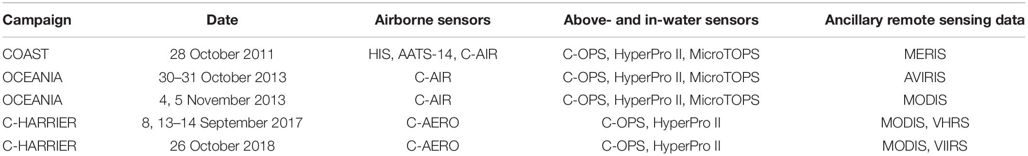
Table 1. Summary of data collection and instrumentation.

NASA COAST initiated the first in a series of airborne CVR concepts for coastal and inland waters and operated in coastal California in 2011, focusing on the greater Monterey Bay region (Figures 1, 2). The goal of the COAST project was to develop and fly a portable airborne sensor suite for NASA science missions addressing the challenges of an optically complex coastal ocean zone in support of research areas such as water quality, ocean productivity and biogeochemistry, coastal landscape alteration, coastal, estuarine, and inland waters ecosystem productivity, atmospheric correction, and regional climate variability (Guild et al., 2011). The COAST instrument suite included a portable Headwall Hyperspectral Imaging System (HIS), the new Coastal Airborne In situ Radiometers (C-AIR) bio-optical radiometer package, and the 14-Channel Ames Airborne Tracking Sun (AATS-14) photometer enabling contemporaneous observations over the same water target for deriving L_W(λ) and relevant aerosol optical depth (AOD) to support atmospheric correction schemes. The instrument integration design and flight planning addressed competing instrument observation requirements and solar geometry to optimize instrument measurements. The COAST flight demonstrations advanced opportunities for aquatic ecosystem research and coastal ocean color CVR capabilities by providing a unique airborne payload optimized for remote sensing in optically complex waters.

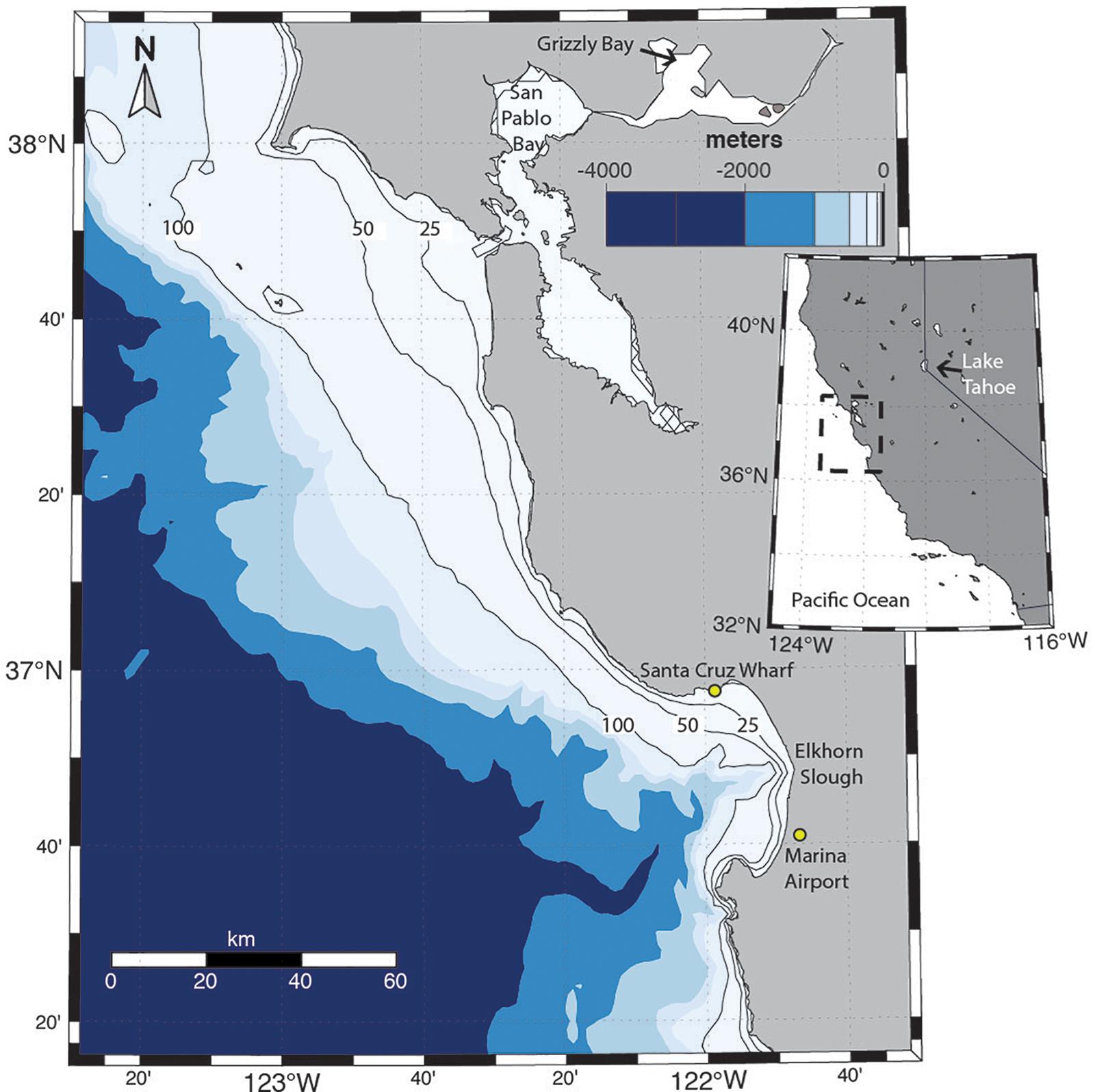
Figure 1. Map of bathymetry and California study site locations of Monterey Bay including Santa Cruz Wharf and Elkhorn Slough, San Pablo Bay, Grizzly Bay, and Lake Tahoe (inset map). The nearby Marina Airport is also identified where the NPS TO is located.

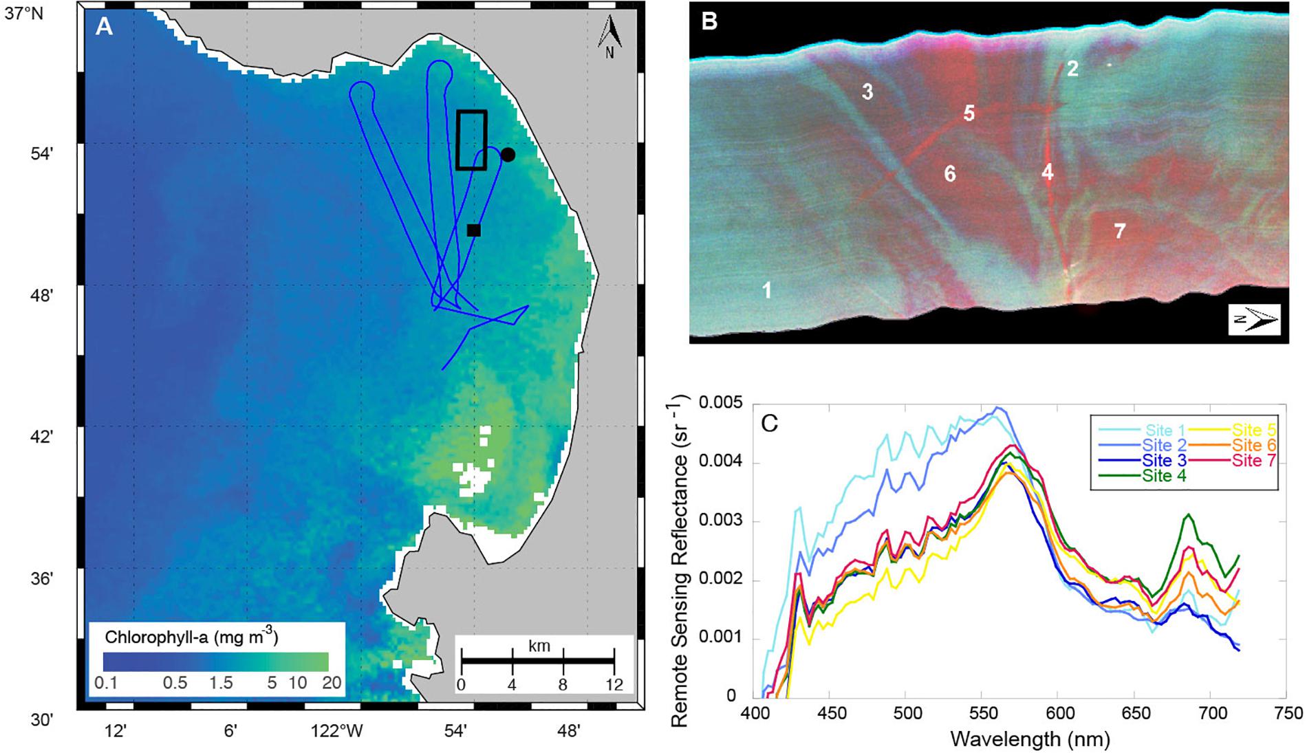
Figure 2. Monterey Bay, CA was the primary target for the airborne missions. (A) The MERIS chl a image from 28 October 2011 (COAST), with the LSA AATS-14 lines (blue) and the “red tide” (CST17; solid circle) and M0 (CST18; solid square) stations. The rectangular box denotes the region depicted in (B), showing the HIS data as an RGB composite, with red indicating high chlorophyll. (C) The spectra from the labels 1–7 in (B) from the HIS. The water depths for these seven sites range from approximately 18 to 25 m.

The 2013 NASA OCEANIA campaign extended the COAST project to focus on apparent optical properties (AOPs) derived from the in-water Compact-Optical Profiling System (C-OPS) built with microradiometers by Biospherical Instruments Inc. (BSI) and from C-AIR flown in COAST aboard the NPS TO aircraft and also built with BSI microradiometers. The OCEANIA project was designed to assess CVR capabilities in support of high-altitude airborne simulation of satellite observations. Flight planning at lowest safe altitude (LSA, e.g., 30 m) used flight headings into and out of the principal solar plane during optimal sun elevation to reduce glint, which were coordinated with field measurements and timing of high-altitude aircraft and satellite overpasses, as well as established flight protocols supporting CVR for the radiometers. Both COAST and OCEANIA utilized a sensor-web network approach to enable simultaneous measurements in support of CVR exercises for satellite coastal ocean color products.

The 2017 and 2018 C-HARRIER campaigns built on the technological development and integration of multiple sensors initiated in COAST and OCEANIA CVR activities. The airborne radiometer suite was upgraded to the Compact-Airborne Environmental Radiometers for Oceanography (C-AERO), which was built with the latest generation of BSI microradiometers (Hooker et al., 2018a). The in-water validation data were obtained with a C-OPS instrument equipped with the Compact-Propulsion Option for Profiling Systems (C-PrOPS) accessory, which adds two small digital thrusters to the backplane so it can be maneuvered independently (Hooker et al., 2018a). The thrusters improve the planar and solar geometry of the light apertures, as well as increasing surface loitering while decreasing descent rate. The net effect of these improvements is a vertical sampling resolution (VSR) that is frequently 1 mm or less (Hooker et al., 2020), whereas C-OPS without C-PrOPS typically has a VSR of 1 cm (Hooker et al., 2013).

The C-AERO instrument suite incorporated increased spectral range to collect data at longer wavelengths, a shroud to eliminate stray light, faster data sampling (from 15 Hz in the 2017 mission to 30 Hz in the 2018 mission) to better discretize surface glint from oblique wave facets, and advanced instrument characterization to improve data processing capabilities by using a novel synthetic dark correction approach (c.f. Kudela et al., 2019 and see section “Implementation of Synthetic Dark Corrections for the C-HARRIER Mission”). The increased data acquisition rate of C-AERO enables a rich collection of CVR data within a single satellite pixel as well as more validation data coverage of smaller water targets (e.g., lakes, rivers, and deltas). C-HARRIER will ultimately include a novel airborne sun photometer, also built with microradiometers, called the Sky-Scanning Sun-Tracking Airborne Radiometer (3STAR), thus completing the development of a sensor-web in which radiometric observations can be conducted for airborne, above-water, and in-water modalities using the same hardware and software suite.

Here we document the evolution of the various sensor suites used for COAST, OCEANIA, and C-HARRIER, including mission planning, operational success, and challenges, and the path toward a fully integrated sensor suite. We highlight specific science applications using these data to underscore how an airborne CVR observatory can be used to understand coastal and inland water quality and provide recommendations for airborne missions in support of aquatic remote sensing, including calibration and validation of existing and future satellite platforms.

Materials and Methods

The methodology development for this airborne CVR capability was enabled through a NASA mission training activity, subsequent innovation funds to advance focused instrument investigation, and ultimately maturing airborne instrument technology and flight demonstrations over varying water types for science missions. These separate projects advanced the airborne CVR methodology through the team members’ expertise in instrument development and ocean biology, ecology, and optics to align science measurement objectives to instrument specifications (Guild et al., 2011, 2019). Further, flight planning on a relevant aircraft to meet science objectives and instrument observation requirements was critical to the success of data acquisition. The following outlines the methodology steps and advances made through each project mission in development of the airborne CVR capability.

First a review of the science requirements supported selection of instruments, or an understanding of their deficiencies, and included identification of relevant channels of the instrument suite aligned to support legacy and next-generation ocean color satellite capabilities. A Science Traceability Matrix (STM) was used to link science objectives and measurements to instrument requirements and performance and provides a conceptual model of the technology threshold needed to meet the measurement objectives. STM science objectives included measurements of aquatic bio-optical properties over spatial extents from less than 1 m to 10 s of meters over coastal waters to capture dynamic coastal phenomena (e.g., blooms and riverine plumes). Corresponding in-water measurements include both apparent (water-leaving radiances) and inherent (absorption, scattering) optical properties at relevant wavelengths (400–800 nm) aligned with satellites used for ocean color (e.g., MERIS, MODIS). These data products form the basis for science questions by deriving relevant ecological and biogeochemical properties from the high-quality water-leaving radiances. Instrument specifications and performance requirements were established in the STM and instruments were evaluated to meet instrument requirements.

For the COAST mission training project, the HIS aligned with the instrument spectral range and was an available test instrument provided by the NASA Ames Research Center (ARC) Airborne Sensor Facility. Additionally, the AATS-14 sun photometer exceeded instrument sensor requirements and was selected for having demonstrated science and flight heritage since 1997 for atmospheric chemistry (Livingston et al., 2003; Redemann et al., 2005, 2009; Russell et al., 2007). The microradiometer instruments (Morrow et al., 2010) provided the instrument channel specifications to align with satellite ocean color sensors and were the underlying foundation of a new CVR radiometric package flying for the first time for COAST and remained the consistent primary instrument suite as the basis for the airborne CVR objective. The flight planning for the AATS-14 sun photometer and HIS were well established; however, the microradiometers were new to integration on an aircraft and flight.

Airborne flight planning over optically dark water targets provides unique challenges from the optically bright targets in terrestrial environments (Mustard et al., 2001; Kudela et al., 2019). Flight plans over water must take into consideration the following: (a) sensor field of view (FOV), integration, and data rate; (b) solar elevation and azimuth to optimize the observational geometry and minimize sun glint; (c) weather mitigation (less than 25% cloud cover); (d) calm wind conditions to simplify water surface roughness modeling, reduce white-cap effects, and facilitate in-water validation measurements; (e) flights ± 30 min of satellite overpass to capture dynamic changes in water features; (f) coordination with in situ validation teams (boat and targets); and (g) for flights including an airborne sun photometer, stacked flight transects at high and low altitudes for full column and intervening layer AOD retrievals.

The TO, operated and maintained by the NPS, was used for all flights. It is a non-pressurized turboprop, twin-engine aircraft. The payload capacity of the TO is 680 kg. The platform endurance is about 5 h in a fully loaded weight configuration. The practical mission ceiling is 5,486 m, or 3,658 m without crew requiring oxygen. Instruments may be installed in racks inside the cabin where a well-characterized community inlet delivers ambient air samples, or in pods either suspended by wing-mounted pylons or mounted on a hard point on the cabin roof. Optical ports and window options for integration are located in certified portals, as well as in the fuselage underside and cabin roof. The NPS has aircraft facility instruments providing position, navigation, time, altitude, groundspeed, heading, pitch, roll, true airspeed, total temperature, dew point, static pressure, dynamic pressure, surface temperature, sky temperature, true wind speed, and wind direction.

COAST Mission Overview

For this study, the COAST project serves as the prime mission model with subsequent extension missions that advanced technical capabilities and methodology in support of improved data quality from airborne observations for aquatics research. The COAST project integrated an instrument suite onboard a platform flown over a location wherein the latter two were trade-study-selected. Examining these trade spaces provided key training opportunities for the team, reflecting typical NASA science flight mission early-phase activities. Following NASA’s procedural requirements for missions, the COAST project passed systems engineering and process requirements of Systems Requirements Review, Preliminary Design Review, Critical Design Review, Airworthiness and Flight Readiness Review, and Flight/Mission Readiness Review. This process established the development and integration of the first airborne end-to-end package for simultaneous measurements of ocean color (modified imaging spectrometer), AOD and water vapor column content (sun photometer), and aquatic bio-optical measurements (fixed-wavelength radiometer package) with the airborne components flight-capable on a variety of airborne platforms. All instruments use inputs from an associated precision navigation system during flight, or the onboard cabin navigation data for post-processing after flight. This first deliverable, therefore, provided a fully operational, integrated, and portable airborne instrument suite optimized for coastal and inland water airborne missions.

Flight planning with instrument science and ocean color scientist team members yielded flights that demonstrated CVR protocols (Hooker et al., 2007) for coastal ocean and inland water color through airborne campaigns of the HIS, AATS-14 sun photometer, and C-AIR microradiometer package flown in coordination with satellite and in situ observations from ships. The flights produced high spatial resolution (5–10 m), atmospherically corrected and geolocated ocean-color products calibrated to at-sensor radiances and post-processed to derive L_W(λ). The primary CVR products from the C-AIR radiometers are L_W(λ) and the corresponding normalized forms, e.g., the remote sensing reflectance (R_rs); there are numerous applications for these data to produce biogeochemically meaningful products for the coastal ocean as well as inland waters.

COAST Airborne Platform and Instrumentation

The 2011 COAST mission flew at altitudes between approximately 30 and 1,829 m on the NPS TO platform on 28 October 2011 over northern Monterey Bay, California (Figures 1, 2).

The complete COAST flight system included three main instruments, a prototype portable Headwall HIS, AATS-14, and C-AIR, with ancillary supporting instruments (Table 1). Sea-truth instrumentation included a MicroTOPS II sun photometer (Solar Light Inc.), C-OPS (BSI), a HyperPro II hyperspectral profiling radiometer (Satlantic), and ancillary supporting instruments including an inherent optical properties (IOP) package consisting of an ac-s (WETLabs), HydroScat-6 (HOBI Labs), and a Conductivity, Temperature, Depth (CTD) instrument (SeaBird Scientific). A detailed comparison of the in-water instruments is provided in Bausell and Kudela (2019) and is not further described here.

Hyperspectral Imaging System

The prototype HIS is a concentric push broom hyperspectral imager of the Offner design optimized in the blue region of the spectrum for marine and freshwater targets. The system was further customized for ocean imaging with a cooled, blue-enhanced charge-coupled device array with 600 × 800 elements and was thermo-electrically cooled to −30°C for increased sensitivity and radiometric stability. The HIS is nadir pointing and mounted on a plate integration design with attachment structures to the seat rails over the nadir port. The HIS was flown at 1,828 m to acquire data at approximately 4 m ground spatial resolution (GSR) with a spectral range of 380–760 nm.

14-Channel Sun Photometer

The AATS-14 measures direct solar-beam transmission (T) at 14 discrete wavelengths from 354 to 2,139 nm, yielding AOD at 13 wavelengths and water vapor column content using T at 940 nm. Azimuth and elevation motors controlled by differential sun sensors rotate the tracking head, keeping the detectors normal to the solar beam. AATS-14 is integrated in a zenith port and on a seat rail mounted truss. AATS-14 has been used extensively to test and improve AOD retrievals by MODIS, SeaWiFS, Multi-angle Imaging SpectroRadiometer (MISR), and many other satellite sensors (Hsu et al., 2002; Livingston et al., 2003; Redemann et al., 2005, 2009; Russell et al., 2007), and to test water vapor retrievals by the Atmospheric Infrared Sounder (AIRS) and MODIS (Livingston et al., 2007). AATS-14-measured AODs have successfully been used in atmospheric correction of satellite data (Spanner et al., 1990; Wrigley et al., 1992).

Airborne Radiometers

Coastal Airborne In situ Radiometers was a new airborne radiometer instrument package flown for the first time for the COAST mission in 2011. Based on microradiometers (Morrow et al., 2010), like C-OPS, C-AIR consists of three 19-channel radiometers: one measuring global solar irradiance (E_s) and fitted with a cosine collector, plus two radiance instruments oriented to measure the indirect sky radiance (L_i) and the total surface radiance (L_T). The spectral range of each 19-channel radiometer bundle includes selected 10 nm channels centered around 320, 340, 380, 412, 443, 490, 510, 532, 555, 589, 625, 670, 683, 710, 780, and 875 nm, seven of which match satellite ocean color (MODIS) bands. The sampling data rate was 15 Hz. Application-specific sensors are included such as UV-bands for CDOM or atmospheric correction, bands targeting phycocyanin and phycoerythrin pigments for flights over reservoirs and terrestrial waters (blue-green algae detection), or bands targeting natural fluorescence (for red tide, high sediment load, and primary production applications). The microradiometer detectors have 10 decades of dynamic range and are sensitive enough to detect moonlight in global irradiance. The physical FOV radiance instrument is 2.5° full-angle and 0.7° slope angle. The E_s and L_i radiometers are mounted within a fairing on top of the aircraft and the L_i radiometer is mounted 40° off zenith, normal to the path of the aircraft. The L_T radiometer is mounted at 40° off nadir, pointed normal to the path of the aircraft, and located alongside the imaging spectrometer in a seat rail structure in an underside nadir port. This configuration eliminated any competing observation requirements between the HIS and C-AIR during flight.

COAST Flight Plan

Flight planning considered the FOV of each instrument and integration on the aircraft. To optimize observations from the hyperspectral imager and radiometer, the aircraft was flown into and out of the principal solar plane and 30–45° solar elevations to avoid sun glint. For the Monterey Bay coastal region in California, this enabled 2–3 h flight windows in the morning and afternoon around solar noon in October. Flight lines were flown in parallel at 1,829 m and spaced with 20% overlap for the HIS. The C-AIR L_T radiometer, pointing 40° from nadir, was pointing at the next adjacent line flown or the previous line flown depending on the heading. LSA flights supported the AATS-14 sun photometer and radiometers observations. Approximately every 20 min, the aircraft spiraled down in concentric circles to LSA and then flew a line under the high-altitude lines and then spiraled up in concentric circles to continue the high-altitude lines. These flight spirals, from high altitude lines down to LSA and back to the high-altitude flight lines, sampled the full atmospheric column and intervening layer for AOD retrievals. Pilots controlled aircraft pitch to not exceed radiometer tolerance requirements which also optimized the hyperspectral imager observations. Flights over Monterey Bay included flight restrictions. The NPS TO was permitted to fly at 30 m altitude outside one nautical mile (including National Marine Sanctuary) from shore and 152 m over vessels.

OCEANIA Mission

The 2013 OCEANIA mission, extended the COAST project to focus on AOPs from in-water (C-OPS) and from the TO airborne platform (C-AIR) to evaluate CVR capabilities in support of high-altitude airborne simulation of satellite observations. OCEANIA did not include the HIS or AATS-14 sensors. C-OPS was upgraded to include small digital thrusters (Hooker et al., 2018a) that improve the VSR to 1 mm or less (Hooker et al., 2020). Driving requirements for flight planning emphasized C-AIR observations without competing requirements from another sensor, as experienced with AATS-14 in COAST and C-AIR E_s, L_i, and L_T radiometer configuration and integration was unchanged. Given successful data acquisition associated with flight planning for COAST, C-AIR was flown at LSA over Monterey Bay at approximately 30 m (150 m over vessels) as well as at 305 m altitude on the NPS TO. Flight headings remained into and out of the sun with 30–45° solar elevations. The low altitude flight plans minimized effects of AOD on C-AIR L_W(λ) derivations consistent with the COAST mission. OCEANIA was flown on 30–31 October and 5 November 2013. The 31 October 2013 flight was coordinated with the Hyperspectral Infrared Imager (HyspIRI) Airborne Preparatory Campaign, which provided coincident imagery from the Airborne Visible Infrared Imaging Spectrometer (AVIRIS) sensor aboard the NASA ER2 platform at approximately 19,810 m (c.f. Palacios et al., 2015).

C-HARRIER 2017 and 2018 Missions

The 2017 NASA C-HARRIER campaign collected measurements in the San Francisco Bay Delta, northern Monterey Bay and Pinto Lake on 8 September, Lake Tahoe on 13 September, and northern Monterey Bay and Pinto Lake on 14 September 2017. The same instrument suite was used as for OCEANIA, but the C-AIR system was upgraded to use C-AERO. As described in Kudela et al. (2019), the principal differences between the two embodiments are that the above-water C-AERO instrument suite has wavelengths spanning 320–1,640 nm (SWIR channels 1,020, 1,245, and 1,640 nm with 10, 15, and 30 nm bandwidths, respectively). This allows for atmospheric correction studies that emphasize long wavelengths. C-AERO includes a shroud to eliminate sun glint in SWIR channels. The sampling frequency remained at 15 Hz. Data were collected from the NPS TO at LSA (approximately 30 m above the water surface). For the 2018 NASA C-HARRIER mission, the C-AERO L_T radiometer was upgraded to a 30 Hz data sampling rate. This upgrade enables additional valid data points following data filtering of sub-optimal airborne data collection and rejection of glint-contaminated data. The resultant data collection increases statistical robustness for 1% radiometry requirements for vicarious calibration and enables a greater number of observations of small water targets such as small lakes, rivers, and estuaries.

Ancillary Imagery

For the scheduled mission flight date windows, available satellite overpass timing options for MERIS (operational for COAST only), MODIS, VIIRS, Landsat 8 OLI, and Sentinel-2 MSI were identified for flight planning purposes. Based on requirements of flights within 30 min of satellite overpass, data from COAST, OCEANIA, and C-HARRIER were compared to contemporaneous imagery from the MERIS sensor, MODIS, and from AVIRIS flown as part of the NASA HyspIRI Airborne Preparatory Campaign (Hochberg et al., 2015; Lee et al., 2015) (Table 1). Data were accessed as Level-1A (L1A) radiances and Level-2 (L2) atmospherically corrected water-leaving radiance products from the NASA repositories. Details of the atmospheric corrections applied are provided in Section “Data Processing.”

Field Sites and in situ Measurements

Our primary coastal field sites are the northern part of Monterey Bay, CA (Figure 1) with secondary sites including Lake Tahoe and San Pablo, Grizzly Bays located in the northern San Francisco Bay. Based on past project experience and typical conditions, a fall flight window maximized data collection days, minimized cloud cover, and provided a range of scientifically interesting features including tidal exchange with Elkhorn Slough (a tidally driven coastal estuary along the Monterey Bay), red tides, fall transition, upwelling versus oceanic conditions, and, potentially, a “first flush” rain event. Actual observations focused on bloom events as both time periods (2011 and 2013) corresponded with seasonally low river flow with no observed salinity anomalies indicative of river plumes at our field sites. Monterey Bay is well characterized oceanographically, provides rich historical and ongoing observations, and has been used in the past for CVR airborne operations (e.g., Ryan et al., 2005a,b, 2008, 2009, 2010; Dierssen et al., 2006; Davis et al., 2007; Chien et al., 2009) including the October 2011 NASA COAST mission (Figure 2) (Guild et al., 2011). In-water validation data were collected aboard the R/V John Martin for COAST and OCEANIA, and from the Santa Cruz Municipal Wharf for C-HARRIER. Instrumentation (Table 1) included the C-OPS and HyperPro II profiling radiometers, MicroTOPS II sun photometer, and ancillary measurements of water quality parameters including total chlorophyll a (TChl a; Van Heukelem and Thomas, 2001), phytoplankton composition via microscopy (Lund et al., 1958), CDOM (Hooker et al., 2020), IOP, and standard oceanographic parameters (temperature, salinity) as described in Bausell and Kudela (2019) and Hooker et al. (2020). Suspended Particulate Material (SPM) was not collected, but a United States Geological Survey (USGS) cruise in San Francisco Bay provided a range of concentrations from the same time period of 14.6–126.3 mg L^–1 (n = 6) for San Pablo and Suisun bays (Grizzly Bay is in northern Suisun; Figure 1).

Data Processing

The radiometric and ancillary data were processed using the Processing of Radiometric Observations of Seawater using Information Technologies (PROSIT) software package (Hooker et al., 2018b) to provide estimates of L_W and R_rs from above- and in-water measurements (Hooker et al., 2018c). As described in Kudela et al. (2019), a full atmospheric correction is not applied given the low flight altitude for OCEANIA and C-HARRIER, but skylight reflectance is removed as per standard NASA above-water reflectance protocols. For COAST, the HIS data were processed using both Tafkaa Tabular, hereafter referred to as Tafkaa, and the vector version of the Second Simulation of the Satellite Signal in the Solar Spectrum (6SV). The 6S code generally is used for atmospheric correction to obtain top of atmosphere (TOA) estimates of radiance and is not optimized to retrieve target water reflectances. Our use of 6SV to perform inverse modeling to obtain a target water reflectance has been used for similar purposes in some aquatic remote sensing studies (e.g., Bélanger et al., 2007; Allan et al., 2011). The aquatic hyperspectral community uses both correction algorithms, e.g., Palacios et al. (2015) corrected high altitude airborne imagery using Tafkaa, and Vanhellemont and Ruddick (2015) generated lookup tables using 6SV. Tafkaa is an atmospheric correction algorithm based on the Atmospheric Removal (ATREM, 4.0) algorithm. In this study, Tafkaa ingests at-sensor radiance of the entire image from the HIS and solves for a number of water-leaving quantities. For the purpose of this study, we used the remote sensing reflectance (R_rs) output. For complete details of the algorithm, see Gao and Davis (1997), Gao et al. (2000), and Montes et al. (2001, 2003). 6SV computes the scattering and absorptive effects of the particles and gases in the atmosphere in order to model the atmosphere from the target reflectance to the sensor (forward modeling approach) or to remove the atmospheric radiance from the at-sensor radiance (inverse modeling approach) to obtain surface reflectance. For the purposes of this study, 6SV was used in the inverse modeling approach, with R_rs derived through division of the dimensionless reflectance by pi following Eq. 3 in Allan et al. (2011). For complete details related to computations used by 6SV, see Vermote et al. (1997), Kotchenova et al. (2006), and Kotchenova and Vermote (2007).

Satellite (MERIS) imagery were processed by the NASA Ocean Biology Processing Group (OBPG) and were accessed as L1A and L2 files. MODIS utilized L2 products with no modification to the standard atmospheric correction. For comparison with the COAST data, the MERIS imagery were reprocessed from L1A data using SeaDAS (v7.3.2). Reprocessing included use of directly measured atmospheric components by applying a fixed AOD model with measured AOD and column water vapor from the AATS-14 LSA dataset (Figures 3, 4). For the HIS data, a sensitivity analysis was performed using both Tafkaa and 6SV. For this analysis, the at-sensor radiance was atmospherically corrected using three atmospheric models (Coastal, Coastal-a, and Maritime) with AOD and column water vapor values from the NASA OBPG processing, MicroTOPS, and AATS-14 (Figure 5). MODIS Aqua data were also examined for indications of upwelling-induced suspended sediments (e.g., Ryan et al., 2012) using the Particulate Inorganic Carbon (PIC) standard product; there was no indication of elevated suspended sediment concentration (SSC) at any of our sites.

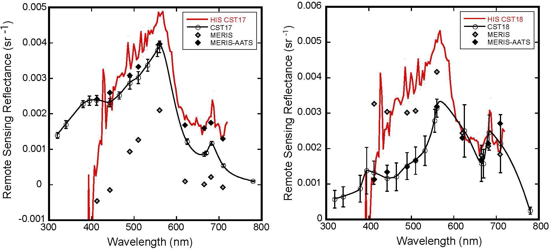
Figure 3. Remote sensing reflectance (R_rs, sr^{– 1}) is plotted for CST17 and CST18 stations, for the HIS (red line), C-OPS in-water profiler (open circles), and MERIS with standard atmospheric correction (open diamonds) and with AATS-14-derived atmospheric correction (solid diamonds). Error bars on the C-OPS data indicate one standard deviation from three consecutive casts.

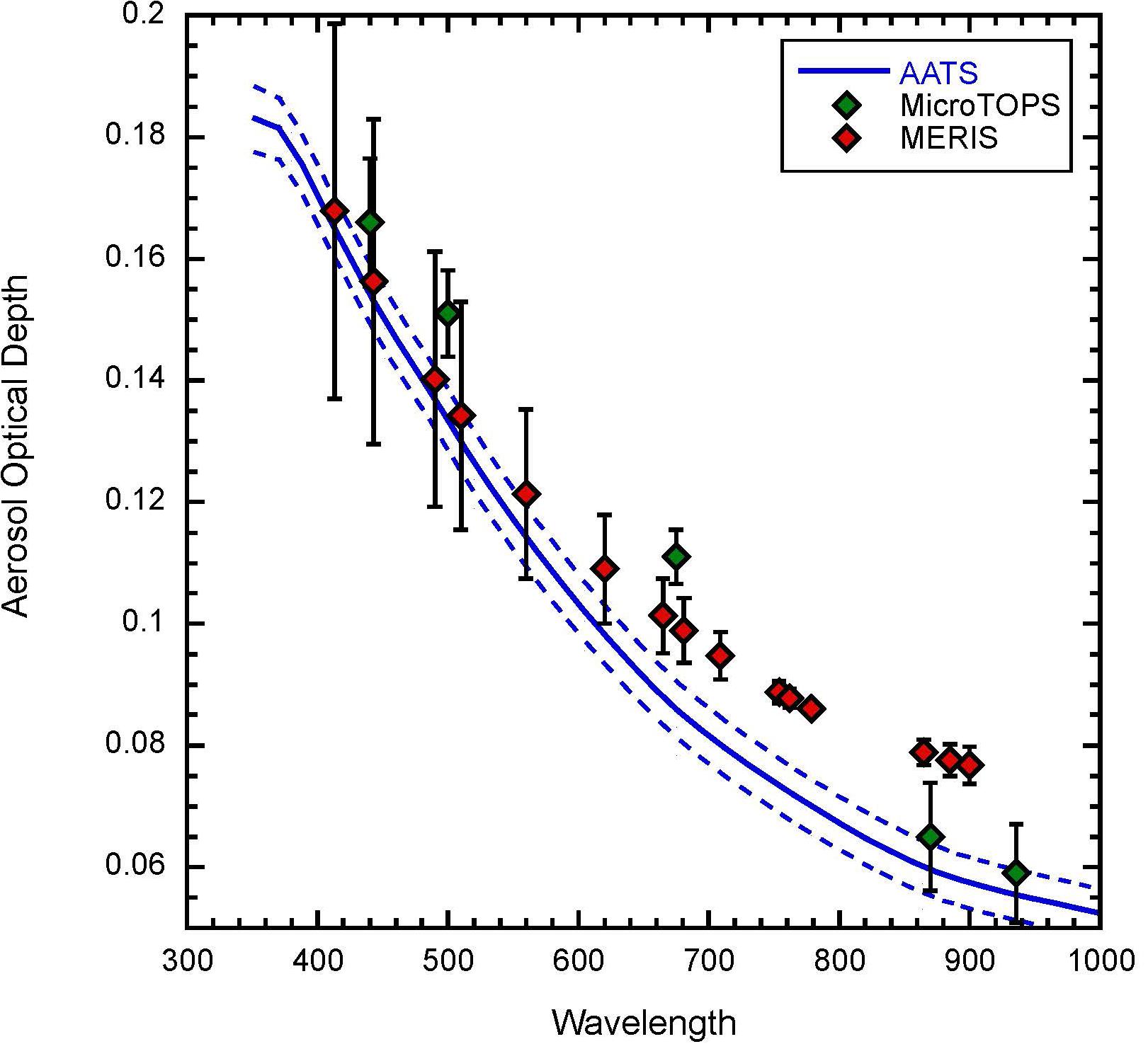
Figure 4. Aerosol optical depth (AOD) derived from the average of all LSA AATS-14 measurements (blue), the average MicroTops II values for two stations, CST17 and CST18 (green), and the default MERIS AOD from SeaDAS parameters (red). Error bars indicate standard deviations for the two stations (green) and for the full MERIS image (red).

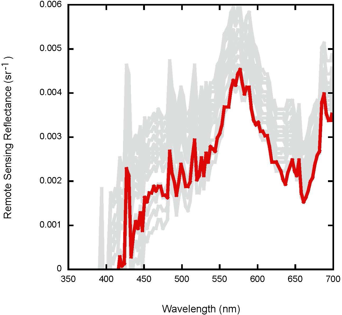
Figure 5. A sensitivity analysis of the atmospheric correction for CST18 from the COAST 2011 mission was performed. The red line indicates the best retrieval (compared to C-AIR and C-OPS) from HIS, while the gray lines indicate retrievals using three atmospheric models in Tafkaa and 6SV with measured AOD values. The best fit falls within the range of reasonable spectra, but without direct measurement of in-water (C-OPS) or LSA data (C-AIR), there is no basis for quantitatively selecting the best spectrum.

Implementation of Synthetic Dark Corrections for the C-HARRIER Mission

A difficulty with autonomous systems, like airborne instrument suites, is the radiometer apertures are not accessible during flight. Consequently, if environmental parameters change significantly with respect to pre- or post-flight conditions when the apertures are accessible, new more representative dark currents cannot be measured. Because dark currents are an order-one term in the calibration equation, accurate dark measurements are a requirement for maintaining an uncertainty budget. The traditional method for measuring dark currents (Hooker, 2014) is to cover the apertures of the radiometers with opaque caps and then to collect dark current observations for each microradiometer gain stage (nominally three). Typically, 1,024 data records are obtained at each gain stage, so quality assurance statistics can be obtained.

A synthetic or predictive dark current (PDC) was developed for each C-AERO radiometer based on a laboratory characterization of the individual microradiometers in each instrument. The laboratory characterization subjected each instrument to an operational range of parameters inside an environmental chamber while acquiring dark currents. The high and low values for each parameter range were based on the performance specifications of the instruments, e.g., temperature ranged from −2 to 40°C. The PDC was validated for the flight certified C-AERO instrument suite using a combination of airborne data and field trials, with the latter obtained with a manual pointing system (Hooker, 2014).

Predictive dark current dark characterization can be applied in three different configurations, based on the environmental parameters for the time period involved, as follows: 1. Equivalent pre- and post-flight caps dark files (called equivalent darks); 2. Along-track flight segment dark files at a temporal interval define by the operator, e.g., 15, 30, 45, and 90 s (called segment darks); and 3. Sample-by-sample corrections at instrument sampling rates of 15 or 30 Hz (called sample darks). The three configurations are evaluated using a combination of airborne and field data partitioned in the spectral domain, as follows: (a) 300–400 nm, UV; (b) 400–600 nm, BGr; (c) 600–700 nm, Red; (d) 700–800 nm, NIR1, (e) 800–900 nm, NIR2, and (f) 900–1,700 nm, SWIR.

Results

Data are presented sequentially from the COAST, OCEANIA, and C-HARRIER airborne campaigns (refer to Table 1 for airborne, field, and available high altitude and satellite data). Presented results were chosen to highlight mission accomplishments and the iterative improvements in the sensor-web approach.

COAST 2011

Data were successfully collected on 28 October 2011 over northern Monterey Bay (Figure 2A). The day of the overflight had calm seas and low winds, with good atmospheric visibility. At that time, there was a large “red tide” present in the bay (Figure 2B), with surface TChl a samples ranging from 4.8 to 75.0 mg m^–3. The bloom was dominated by the dinoflagellate genera Akashiwo, Ceratium, and Prorocentrum with TChl a at Stations 17 and 18 (Figure 2A) of 6.8 and 52.8 mg m^–3 and site location depths of 24 and 84 m, respectively. Figure 1 provides bathymetry for the entire region. The biomass was distributed heterogeneously (Figure 2B), with substantial spatial and temporal variability and corresponding variability in R_rs (Figure 2C). Despite the heterogeneity, comparable matchups between in-water and remotely sensed instrumentation were achieved, with a MERIS overpass at 1855 (UTC), AATS-14 and HIS data collected over the two stations at 2022 and 2024, and in-water observations at 1852 and 2040, or within less than a 2 h window (Figure 3). SPM samples were not collected but given the lack of river plumes or upwelling-induced suspended sediments, it was assumed that SPM was a minor contribution to the optical signals. The elevated red (approximately 555 nm) peak observed at several sites (Figures 3, 5, 6) was attributed to high algal biomass rather than SPM, which typically shifts further toward 600 nm with increasing concentration (Dierssen et al., 2006).

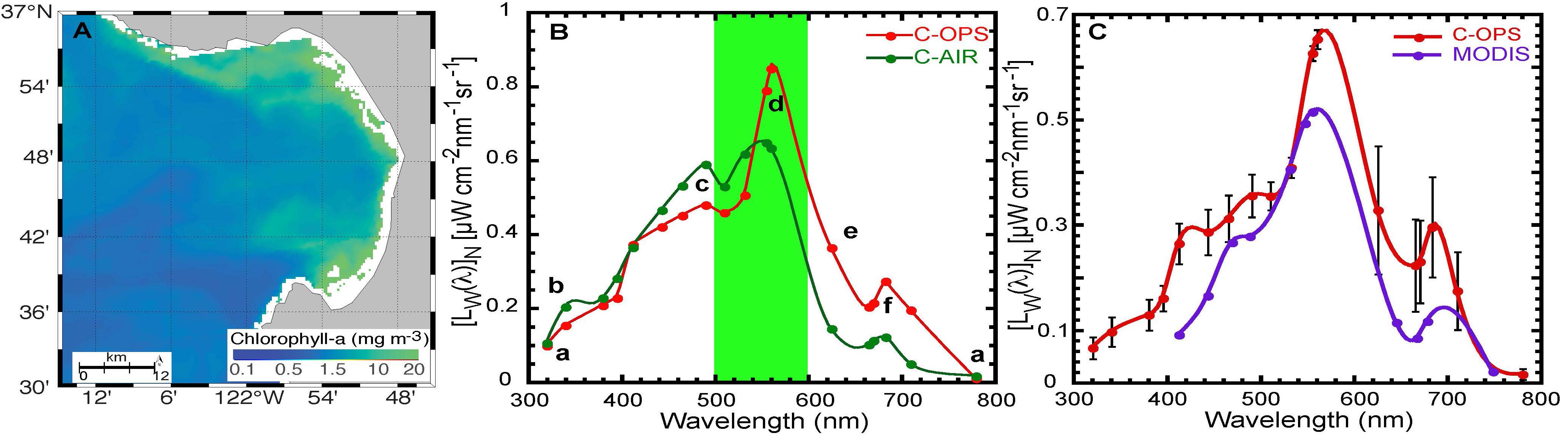
Figure 6. MODIS Aqua Chl a from 5 November 2013 (OCEANIA) is shown in (A), processed at 250 m resolution, with a comparison of C-OPS (in-water) and C-AIR (airborne) within the red tide in (B), and the corresponding C-OPS versus MODIS data in (C) processed at 1 km resolution. Error bars in (C) represent the standard deviation of three consecutive C-OPS profiles. Station location is indicated in Figure 2A (solid circle).

Direct comparisons of R_rs between the C-OPS, HIS, and MERIS showed similar spectral shapes, but with large discrepancies for several wavelengths (Figure 3). Specifically, MERIS data obtained directly from NASA exhibited severe underestimates (including negative reflectances) at Station 17 and overestimates at Station 18, while HIS generally overestimated R_rs compared to C-OPS with significant sensor noise and very poor sensitivity and performance for blue and red spectral end members. To assess whether the remotely sensed data could be improved with a regionally tuned atmospheric correction, the MERIS data were reanalyzed using a fixed aerosol model and directly measured AOD and column water vapor from both a MicroTOPS II handheld sun photometer deployed aboard the ship and the average AOD and column water vapor values from LSA flight lines using AATS-14 (Figure 2A and Table 2). While the AOD values were similar between sensors (Figure 4), the overestimation of AOD beyond 600 nm resulted in substantial discrepancies in calculated R_rs (Figure 3), highlighting the utility of coincident airborne AOD measurements.

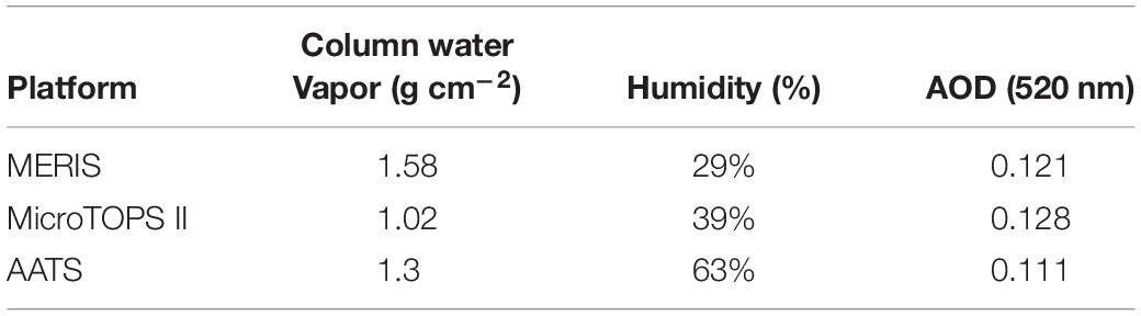
Table 2. Summary of atmospheric parameters used for correction of the HIS imagery.

For quantitative assessment of the data, the relative percent difference (RPD) was calculated for R_rs at the MERIS wavelengths for C-OPS (considered to be the most accurate; Kudela et al., 2019) and MERIS. The average RPD for all MERIS wavelengths was −87% for CST 17 and 18% for CST 18 with standard processing. Using MicroTOPS data improved the RPD for CST 17 but not CST 18, with RPD of 35 and 36%, while the RPD for AATS-14-corrected imagery was 29 and 0.9%, respectively.

For the HIS data, a sensitivity analysis was performed using both Tafkaa and 6SV. For this analysis, the at-sensor radiance was atmospherically corrected using three atmospheric models (Coastal, Coastal-a, and Maritime) with AOD and column water vapor values from the NASA OBPG processing, MicroTOPS, and AATS-14 (Figure 5). While both models produce reasonable values, the R_rs spectra span a considerable range (factor of two) with no ability to a priori identify any particular combination as the “best” solution.

Following the COAST mission, the prototype HIS was removed from the instrument package because significant engineering issues (poor calibration results, not blue-optimized, significant noise, difficulty integrating the data stream) were discovered. C-AIR flew successfully on the TO during COAST but was not collecting adequate time series of data at LSA with optimal headings due to the driving priority of the flight planning for the AATS-14 and was therefore not used for demonstration of the airborne CVR activity during COAST.

OCEANIA 2013

The OCEANIA mission focused on supporting airborne CVR through the collection of coincident data from the TO at LSA using C-AIR and from in-water observations using C-OPS with small digital thrusters. Both instrument packages employ single-channel microradiometers, allowing sensor calibration, data collection, and post-processing to occur using the same workflow and identical hardware components (Hooker et al., 2018a,b,c). Data were again collected over northern Monterey Bay on 5 November 2013 (Figure 6A showing MODIS Aqua Chl a; see also Palacios et al., 2015; Bausell and Kudela, 2019) with clear skies, good visibility, and low winds. TChl a was comparable to COAST with a value of 8.3 mg m^–3. Red tides were prominent in September and October of that year (Palacios et al., 2015), with the dinoflagellate genera Cochlodinium, Prorocentrum, and Ceratium dominating at the OCEANIA station on 5 November 2013. AVIRIS data were acquired over the same location immediately prior to OCEANIA on 31 October 2013, for which the Pajaro River Mouth (PRM) station in Palacios et al. (2015) was coincident with OCEANIA. As noted above, there was no indication of significant concentrations of SPM from the river or from upwelling at these sites.

In-water data were collected with the C-OPS profiler within the red tide (Figure 6). C-OPS data were collected from 2025 to 2032 (UTC) while the closest matching C-AIR data collected at LSA from the TO were collected at 1914, and a MODIS Aqua image was captured at 2110, approximately a 2 h window for all observations. A comparison of data products derived from above- and in-water measurements is presented in Figure 6B, with normalized forms obtained following published NASA Ocean Optics protocols wherein bidirectionally corrected spectra were derived and presented in normalized forms to account for the solar illumination and geometry (Hooker et al., 2002, 2004). Products obtained by deploying C-OPS from a small ship are shown in red and products obtained from the C-AIR instrument on the NPS TO are shown in green. The data compare the nearest in-water station to the nearest airborne observation. The plot shows the in-water data were obtained more substantially inside the red tide, because the highest amplitude peak in the green domain is with the C-OPS data. Six spectral features spanning the entire spectral domain (UV to NIR) demonstrate the good agreement achieved between the two sensor systems: (a) the UV and NIR spectral end members are in agreement; (b) the expected UV shoulder for the type of coastal water sampled is in both spectra, with the C-OPS data showing the anticipated UV suppression from the more intense bloom conditions; (c) the expected blue shoulder for higher productivity coastal water in both spectra, with the in-water data showing greater blue suppression from the more intense bloom conditions; (d) the expected peak in the green domain is in both spectra with the higher in-water peak establishing the C-OPS data were obtained more substantially in the red tide; (e) the expected higher elevation of the red domain for the in-water spectrum (which was obtained in more intense bloom conditions); and (f) the expected fluorescence peak is present in both spectra, with the in-water peak being larger as expected.

Spectra from the MODIS image was comparable to C-AIR and C-OPS (Figure 6C), although it should be noted that the 488 nm band exhibited negative radiance, presumably due to poor atmospheric correction. In contrast to the MODIS data, AVIRIS data collected a week prior (31 October 2013) were unable to produce accurate retrievals of ocean color due to a combination of poor SNR and suboptimal atmospheric correction (Palacios et al., 2015).

C-HARRIER 2017 and 2018

The C-HARRIER 2017 and 2018 missions focused primarily on flight planning and highlight incremental improvements to the C-AERO sensor including a shroud and expanded spectral range from 320 to 1,640 nm. Specifically, sampling rates were increased from 15 to 30 Hz for the 2018 mission for the downward-viewing L_T radiometer (total radiance from the surface). A new “synthetic dark” method was developed to apply dark corrections to the instruments during flight (rather than before and after flight).

In 2017, flight planning was enhanced to include additional sites demonstrating data collection in varying water types and feasibility of sorties to inland waters such as the San Francisco Bay and Lake Tahoe. Grizzly Bay and San Pablo Bay represented the turbid waters of San Francisco Bay. Lake Tahoe represented oligotrophic (e.g., oceanic) conditions, a clear water type.

For 2018, the primary field target was northern Monterey Bay. A short segment was collected near the Santa Cruz Municipal Wharf, and after processing (including the use of synthetic darks) the data were reduced from 30 to 15 Hz and the SNR was calculated as per Kudela et al. (2019) (Figure 7). Absolute values of SNR were comparable but use of the 30 Hz data increased SNR approximately 1–9%, depending on wavelength, with greatest improvement in the NIR and SWIR region (Figure 7). It is also notable that increasing the sampling rate effectively decreases the ground sampling distance (GSD) without adjusting other flight characteristics. In this example, the GSD decreased from 3.4 to 1.7 m at 15 and 30 Hz, respectively, for an LSA of 30 m and a speed over ground of 185 kph.

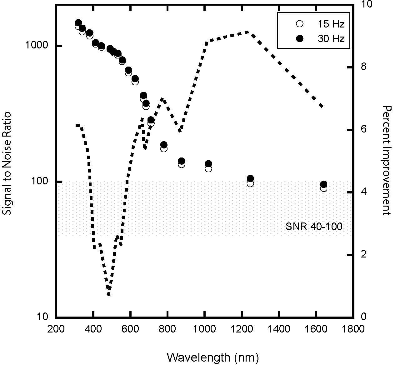
Figure 7. Effective signal-to-noise ratio (SNR) calculated at LSA for C-AERO data over Monterey Bay, CA collected 26 October 2018 (C-HARRIER) with C-AERO at 15 and 30 Hz. The stippled region identifies an optimal SNR of 40–100, while the dashed line provides the percent difference in SNR for 15 versus 30 Hz otherwise processed using the same methods. The percent improvement (as percent increase in SNR when collecting at 15 versus 30 Hz) is shown as the dashed line.

A PDC method described in Section “Implementation of Synthetic Dark Corrections for the C-HARRIER Mission” was used to apply dark corrections to the 2017 and 2018 data collections (Figure 8). Processing existing airborne C-AERO data with caps darks versus equivalent darks results in data products that agree at all wavelengths to within 0.1%. For manually pointed C-AERO data, the use of equivalent darks produces data products that agree with an in-water C-OPS instrument suite as follows: UV −4.2, BGr −2.9, Red −1.7, NIR1 −2.8, and NIR2 7.9%, which is similar to the combined uncertainty for sensor calibration (about 3%) plus temporal variance during station work (5% or less, but without an estimate of spatial variance), except for NIR2. Pearson’s statistical correlation coefficient, ρ, for the two relevant match-up spectra in Figure 8 is shown for the SPB, GB, MB, and LT sites. The overall average value is ρ = 0.991, which means more than 99% of the variance in the shape is explained. These data span a large range of bio-optical complexity, from very blue water (Lake Tahoe) to estuarine waters dominated by both CDOM and non-algal particles (Grizzly Bay). The excellent agreement in spectral shape for all sites translates directly into reduced error for derived products such as chl a that rely on band-ratios (i.e., spectral shape and magnitude). Estimation of the absolute percent difference using the standard maximum band ratio approach yields uncertainty of 5.9% in Tchl a for the data in Figure 8, well within the range of acceptable uncertainty for existing satellite sensors (Kudela et al., 2019).

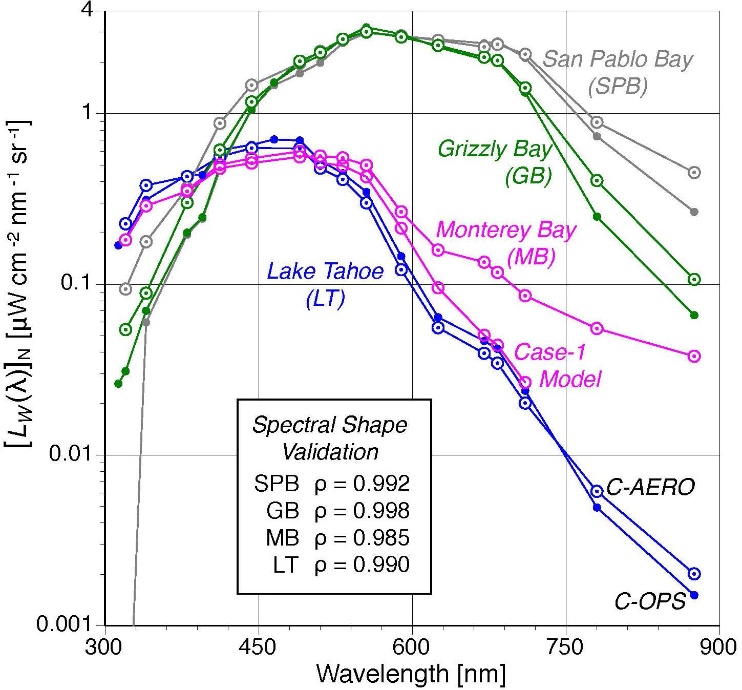
Figure 8. C-AERO was validated using in situ data obtained with a C-OPS equipped with digital thrusters (C-PrOPS) except in Monterey Bay (30 Hz L_T data), wherein a case-1 model was used. The matchups between C-AERO and C-OPS are based on minimizing the distance between the two sampling sites. For the Monterey Bay comparison, the TChl a concentration obtained at the Santa Cruz Wharf was used to derive the case-1 model results and compared to the spatially nearest C-AERO observation. The correlations (ρ) in spectral shape for each site are provided, demonstrating excellent retrieval of spectral information from the airborne observations.

Processing existing airborne C-AERO data with segment darks results in no negative calibrated radiometric values, whereas the use of caps darks (either pre- or post-flight) can produce negative calibrated radiances over dim targets in the middle of a long flight. For the airborne data used herein, the amount of data that is lost due to negative calibrated radiances if caps darks are used is less than 1.8% (no field data is lost for caps darks, because the deployments are relatively short in duration). A larger percentage of the SWIR data is improved by using segment darks. Approximately 3.5% of the data are sufficiently changed by the use of segment darks to influence data products at the 1% level or more. None of the data obtained in other wavelength domains are improved sufficiently to influence data products at the 1% level or more, but this is likely a function of the water bodies that were sampled.

Processing existing airborne C-AERO data with segment darks versus sample darks results in data products that agree at all wavelengths to within 0.2%; the agreement is to within 1% at all wavelengths for field data. The reason for the excellent agreement is due to the relative short time periods used to define a flight segment. The longest flight segment is 90 s, so the opportunity for environmental or performance changes during a flight segment for an aircraft operating at near-constant LSA is small.

Discussion

Aquatic remote sensing provides a cost-effective, synoptic method for deriving information about the ecologically relevant constituents of the coastal ocean (IOCCG, 2000), because ocean color provides a depth integrated measurement of the biotic and abiotic constituents that interact with light in the ocean. What has historically been challenging is partitioning this signal into relevant biogeochemical parameters (Dierssen et al., 2006; Dunagan et al., 2009; Gregg and Casey, 2010; Guild et al., 2011, 2019). The magnitude of L_W is spectrally, spatially, and temporally variable, ranging from very dark values in clear, deep water to very bright values at water’s edge. The spatial (1 km) and temporal (daily) resolution from legacy instruments is of marginal use in coastal waters (Aurin et al., 2013; Dekker et al., 2018). Further, low SNR measurements of L_W in the blue spectral domain contribute to poor discrimination of pigments from CDOM and poor estimates in the UV (Kudela et al., 2019). Continental sources of aerosols and trace gas plumes may not be well represented by atmospheric models used in atmospheric correction approaches. Also, for productive coastal waters, the use of non-zero NIR radiances and poor SNR values complicate atmospheric correction schemes based on SWIR wavelengths (Siegel et al., 2000; Shi and Wang, 2009; Werdell et al., 2010).

NASA Ocean Optics Protocols require CVR uncertainties as follows: calibration data to within 5%, validation data to within 10% error, and research data to within 25% (Hooker and McClain, 2000). A fundamental limitation using historical airborne and satellite data is that sensors such as AVIRIS, the primary instrument (for example) in the HyspIRI Preparatory Airborne Campaign, has poor SNR and calibration issues (Palacios et al., 2015; Thompson et al., 2015), with SNR at 400 nm as low as 20:1, compared to a next-generation requirement of 400:1 for the Plankton, Aerosol, Cloud, ocean Ecosystem (PACE) sensor. Second, in-water calibration data are needed, limiting the improved correction to specific targets (Moses et al., 2012). Next-generation satellite sensors are also required to meet 3.5% absolute accuracy, with 1% absolute radiometry for validation (Hooker et al., 2007), which is challenging at best for existing airborne and satellite platforms (Kudela et al., 2019). A fundamental goal of COAST, OCEANIA, C-HARRIER, and related campaigns was to demonstrate the evolution of the capability to meet these exacting requirements in coastal ocean and inland waters while simultaneously moving away from the traditional paradigm of relying on a limited number of fixed locations for CVR data [e.g., AErosol RObotic NETwork Ocean Color (AERONET-OC), Zibordi et al., 2009].

A primary obstacle for the remote sensing of coastal and inland waters is atmospheric correction. The COAST campaign demonstrated the utility of collecting high-quality atmospheric and oceanic data simultaneously from an airborne platform by collocating a science-grade sun photometer and ocean color radiometers. Traditional processing of MERIS satellite data resulted in both over- and underestimation of R_rs and was greatly improved with the addition of AOD collected either from a fixed platform (MicroTOPS aboard the research vessel) or from the TO. A clear advantage of the airborne approach is that considerable additional spatial information is provided for AOD, as well as an ability to collect columnar atmospheric data by varying flight altitude. The improved horizontal and vertical resolution provided by the airborne perspective is most useful for heterogeneous air masses, which often correspond to inland (i.e., compared with marine) environments.

A sensitivity analysis of the HIS atmospheric correction reinforces the requirement for highly accurate atmospheric information for post-processing of imagery. For this analysis, we focused primarily on calibration and validation and therefore primarily analyzed the data from the two locations where in-water measurements were available. The spatially explicit AOD data, like that from the AATS-14 aboard the TO, would enable future missions coupling a sun photometer with imaging spectrometers to conduct a pixel-by-pixel atmospheric correction, which would presumably greatly improve data collection for any mission study airborne simulation programs supporting PACE, the Surface Biology and Geology (SBG) hyperspectral mission study (Schneider et al., 2019), and the past HyspIRI precursor study (Hochberg et al., 2015), where AVIRIS atmospheric correction issues varied dramatically across a space of a few kilometers for Monterey Bay (Palacios et al., 2015). While the HIS had significant engineering and data processing issues, COAST also highlighted the desirability to capture the two-dimensional structure of the surface ocean to put the more limited shipboard data into spatial context (Figure 2B).

The OCEANIA campaign highlighted the usefulness of a high SNR sensor with expanded spectral range (C-AIR) flown at LSA, relevant to coastal remote sensing. For example, while AATS-14 was not available for OCEANIA, there was also no requirement for atmospheric correction of the C-AIR data at LSA, as demonstrated by the very good agreement between the C-OPS and C-AIR spectra over the red tide (Figure 6B). It was recognized that next-generation sensors for missions such as PACE and SBG would challenge existing CVR instrumentation by requiring radiometric measurements extending into the UV and NIR and shortwave infrared, where legacy instruments are challenged by noise and sensitivity issues (e.g., Kudela et al., 2019). The C-AERO instrument was, therefore, designed around the same microradiometers used in C-AIR but with extended spectral range (320–1,640 nm) and addition of a shroud to reduce long wavelength scattering at the sensor aperture (Hooker et al., 2018a). For C-HARRIER, the C-AERO sensor was further upgraded between 2017 (Kudela et al., 2019) and 2018 by increasing the sampling frequency from 15 to 30 Hz. This effectively decreases GSD while doubling the data volume, allowing post-processing to exclude noisy features such as glint and whitecaps that would be included in the data for instruments sampling at slower rates.

Following OCEANIA, it was also recognized that inexpensive and easy to deploy sun-tracking photometers were lacking, given the high demand and frequent unavailability of systems such as AATS-14. The same microradiometer systems were therefore used to develop a portable fixed-platform system, the Compact-Optical Sensors for Planetary Radiant Energy (C-OSPREy) sun photometer mounted on a tracker with a quad detector, supported by a solar reference (E_s) with a shadow band, documented in Hooker et al. (2018b), and initial development of the microradiometer-based 3STAR sun-tracking photometer, based on the same design and engineering as the C-AIR radiance sensor. The C-OSPREy system was not deployed in Monterey for C-HARRIER, because 3STAR was not flight certified, but is considered to be at NASA technical readiness level (TRL) 9 after successful deployments on multiple campaigns (Hooker et al., 2018c). At this time, all engineering and flight-readiness tests for 3STAR aboard the TO are completed, but 3STAR has not conducted a science mission. Consequently, the capabilities of 3STAR are not evaluated within this manuscript.

With the completion of engineering tests for 3STAR in 2019, all the components for a fully operational coastal in-water and airborne “sensor-web” approach were established. All of the radiometer instruments (C-OPS, CAIR, C-AERO, C-OSPREy, and 3STAR) are based on the same core set of microradiometers (albeit using different generations of microradiometers with C-AERO and C-OSPREy being the most recent) with National Institute of Standards and Technology traceable absolute calibration and 10 decades of dynamic range. This approach is fundamentally different from traditional calibration methods which typically rely on fixed location and custom-built above- and in-water optical sensor packages maintained in one location, e.g., the Marine Optical Buoy (MOBy) and Bouée pour l’acquisition de Séries Optiques à Long Terme (BOUSSOLE) projects (Clark et al., 2003; Antoine et al., 2008, respectively) which cannot be opportunistically deployed across different regions and are generally not optimized for measurement of shallower and more complex inland water bodies. The approach described here provides calibration-level performance for ocean color from fixed platforms as well as airborne observatories; when flown at LSA, the requirement for complex atmospheric correction is removed, while the 10-decade dynamic range allows the same sensors to operate equally effectively in water ranging from extremely clear to highly turbid, including red tides (Hooker et al., 2018a,b,c; Kudela et al., 2019), and across an expanded spectral range that improves algorithm performance for a global range of water bodies (Hooker et al., 2020; Houskeeper et al., 2021). The 15 Hz version of C-AERO already met or exceeded all recommendations for SNR from the aquatic remote sensing community (Kudela et al., 2019), while the recent upgrade to 30 Hz sampling for the downward-viewing (L_T) radiometer has substantially increased the realized SNR for coastal waters. Implementation of the synthetic or predicted darks correction (PDC) improved the radiometric accuracy at all wavelengths, with the greatest improvements at the longer NIR and SWIR wavebands most relevant to atmospheric correction.

A unique capability of this approach is that calibration and validation targets are no longer limited to a handful of ground- or ship-based sun photometer locations. For example, during the C-HARRIER mission, calibration-quality data were collected over a 300 km span covering Monterey Bay, San Francisco Bay, and Lake Tahoe, CA in a matter of days, with the primary limitation being the availability of personnel and instrumentation for the in-water measurements. We estimate that for a similar payload, the TO used in these studies could extend this range to 1,300 km with flight altitudes ranging from LSA to 3,048 m. This capability opens up the possibility of collecting high-quality CVR data nearly anywhere a suitable airborne platform is available, thus providing data quickly and cost effectively from oligotrophic case-1 waters to bright coastal, estuarine, and inland water targets in the same mission, or multiple revisits of the same location to support the calibration and validation of geostationary sensors, e.g., the Geosynchronous Littoral Imaging and Monitoring Radiometer (Geosynchronous Littoral Imaging and Monitoring Radiometer [GLIMR], 2019) instrument recently selected for development. This approach opens the potential for rapidly acquiring calibration-quality data in a variety of environments in consideration of maintaining sites such as MOBy and greatly reducing the time required to generate appropriate datasets that cover the required range of variability (Bailey et al., 2008). Similarly as noted by Mouw et al. (2015), the primary network used for calibration and validation of aquatic atmospheric correction is AERONET-OC which consists of only a handful of locations (Zibordi et al., 2009), has limited spectral bands, and insufficient resolution in the red to NIR for coastal and inland waters. Recent improvements have increased the spectral resolution and range of above-water instrument suites relevant to calibration (e.g., Vansteenwegen et al., 2019), but are still limited by expanded (compared with C-AERO) integration times and by the spatial limitations of a fixed-location approach. Through the development of a microradiometer-based sensor suite, CVR can be achieved for both the aquatic and atmospheric components anywhere in the world that a suitable airborne platform is available.

To summarize, optically complex coastal and inland waters pose unique challenges for remote sensing. The optical heterogeneity of coastal and inland waters is the result of a diversity of influences such as river plumes, algal blooms, benthic habitats, and resuspension of sediments over shallow shelves—all of which can be further influenced by climatic changes, e.g., drought and flooding. Inland waters are predominantly smaller spatial targets and challenging for satellite remote sensing. The overlying atmosphere is also variable due to terrestrial inputs of aerosols (dust, particulates, and smoke), water vapor, and trace gases, while changes in elevation require modification of atmospheric correction protocols. Improved sensor SNR, spectral range and resolution, spatial coverage, and temporal resolution (to capture water circulation dynamics of features) are needed to support aquatic observations and correction of the atmospheric influences on these observations to fill gaps in coastal and inland waters research. While not a focus of this paper, the same instrumentation used herein also meets or exceeds criteria for case-1 open ocean waters. As demonstrated in the evolving airborne microradiometer instruments used in the COAST, OCEANIA, and C-HARRIER missions, such airborne observatories can readily support local coverage of coastal and inland waters and bridge the high-fidelity CVR quality observations to relevant high altitude airborne and satellite observations.

Data Availability Statement

The raw data supporting the conclusions of this article will be made available by the authors, without undue reservation.

Author Contributions

LG served as the principal investigator on the COAST, OCEANIA, and C-HARRIER projects and managed the flight planning and airborne mission flight data collection. LG, RK, and SH contributed to the conception and design of the study. LG and RK wrote the initial draft of the manuscript. RK and SH served as co-investigators on the various NASA projects, participated in data collection for all field campaigns, writing and revision of the manuscript, and preparation of figures. SP participated in field data collection during COAST and OCEANIA, flight planning for OCEANIA, hyperspectral image processing, atmospheric correction sensitivity analysis in Takfaa and 6SV of hyperspectral imagery, and revision of the manuscript. HH participated in data collection during C-HARRIER, processing of field data, preparation of figures, and revision of the manuscript. All authors contributed to the article and approved the submitted version.

Funding

The authors declare that this study received funding from NASA. The funder had the following involvement with the study: missions, advancing the airborne instrument technology, data collection, and data analyses. LG, RK, SH, SP, HH, and NASA ARC, UCSC, University of Miami, and BSI project team members received support from the following NASA Programs: (1) HOPE COAST project by NASA Headquarters (HQ) awards from the Science Mission Directorate (SMD) and Office of Chief Engineer Hands-On Project Experience (HOPE) 2010 Training Opportunity For NASA Personnel; (2) Remote Sensing of Water Quality (NNH12ZDA001N-WATER A.32), Earth Science Division (ESD), SMD (High Quality Optical Observations, H-Q2O, for data analysis of COAST and OCEANIA missions); (3) 2013 NASA-ARC Science Innovation Fund (SIF), NASA HQ Office of Chief Scientist, SMD (OCEANIA mission); (4) 2016 NASA-ARC SIF, NASA HQ Office of Chief Scientist (advancing instrument technology); and (5) Airborne Instrument Technology Transition (NNH16ZDA001N-AITT A.26), ESD, SMD (advancing instrument technology, C-HARRIER missions, and data analyses).

Conflict of Interest

The authors declare that the research was conducted in the absence of any commercial or financial relationships that could be construed as a potential conflict of interest.

Acknowledgments

We would like to recognize John Morrow, Biospherical Instruments, Inc., as one of the original team members who conceived of the airborne CVR competency and provided expertise in the radiometry and aquatic bio-optics science for all the airborne missions presented. Also, we acknowledge the significant contributions of Stephen Dunagan and James Eilers who developed the design and implemented the integration of the airborne instruments flying for the first time or flying in the suite configurations for the first time as well as developing flight plans. This engineering activity was innovative in itself. We would like to thank the two reviewers whose thoughtful review has strengthened the contribution of this manuscript.

References

Allan, M. G., Hamilton, D. P., Hicks, B. J., and Brabyn, L. (2011). Landsat remote sensing of chlorophyll a concentrations in central North Island lakes of New Zealand. Intern. J. Remote Sens. 32, 2037–2055. doi: 10.1080/01431161003645840
Antoine, D., d’Ortenzio, F., Hooker, S. B., Bécu, G., Gentili, B., Tailliez, D., et al. (2008). Assessment of uncertainty in the ocean reflectance determined by three satellite ocean color sensors (MERIS, SeaWiFS and MODIS-A) at an offshore site in the Mediterranean Sea (BOUSSOLE project). J. Geophys. Res. Oceans 113:2007JC004472. doi: 10.1029/2007JC004472
Aurin, D., Mannino, A., and Franz, B. (2013). Spatially resolving ocean color and sediment dispersion in river plumes, coastal systems, and continental shelf waters. Remote Sens. Environ. 137, 212–225. doi: 10.1016/j.rse.2013.06.018
Bailey, S. W., Hooker, S. B., Antoine, D., Franz, B. A., and Werdell, P. J. (2008). Sources and assumptions for the vicarious calibration of ocean color satellite observations. Appl. Opt. 47, 2035–2045. doi: 10.1364/AO.47.002035
Bausell, J., and Kudela, R. (2019). Comparison of two in-water optical profilers in a dynamic coastal marine ecosystem. Appl. Opt. 58, 7319–7330. doi: 10.1364/AO.58.007319
Bélanger, S., Ehn, J. K., and Babin, M. (2007). Impact of sea ice on the retrieval of water-leaving reflectance, chlorophyll a concentration and inherent optical properties from satellite ocean color data. Remote Sens. Environ. 11, 51–68. doi: 10.1016/j.rse.2007.03.013
Brezonik, P. L., Olmanson, L. G., Finlay, J. C., and Bauer, M. E. (2015). Factors affecting the measurement of CDOM by remote sensing of optically complex inland waters. Remote Sens. Environ. 157, 199–215. doi: 10.1016/j.rse.2014.04.033
Chien, S., Doubleday, J., Tran, D., Thompson, D., Mahoney, D., and Chao, Y. (2009). “Towards an autonomous space in-situ marine sensorweb,” in Proceedings of the AIAA Infotech@Aerospace Conference, 6-9 April 2009, Seattle, WA.
Clark, D. K., Yarbrough, M. A., Feinholz, M., Flora, S., Broenkow, W., Kim, Y. S., et al. (2003). “MOBy, a radiometric buoy for performance monitoring and vicarious calibration of satellite ocean color sensors: measurement and data analysis protocols,” in Ocean Optics Protocols for Satellite Ocean Color Sensor Validation, Revision 4, Volume VI: Special Topics in Ocean Optics Protocols and Appendices, eds J. L. Mueller, G. S. Fargion, and C. R. McClain (Greenbelt, MD: NASA Goddard Space Flight Center), 3–34.
Davis, C. O., Kavanaugh, M., Letelier, R., Bissett, W. P., and Kohler, D. (2007). “Spatial and spectral resolution considerations for imaging coastal waters,” in Proceedings of the SPIE 6680, Coastal Ocean Remote Sensing, San Diego, CA.
Dekker, A. G., Pinnel, N., Gege, P., Briottet, X., Court, A., Peters, S., et al. (2018). “Feasibility study for an aquatic ecosystem earth observing system, version 2.0,” in Proceedings of the Committee on Earth Observation Satellites (CEOS), Canberra.
Dierssen, H. M., Kudela, R. M., Ryan, J. P., and Zimmerman, R. C. (2006). Red and black tides: quantitative analysis of water-leaving radiance and perceived color for phytoplankton, colored dissolved organic matter, and suspended sediments. Limnol. Oceanogr. 51, 2646–2659. doi: 10.4319/lo.2006.51.6.2646
Dunagan, S., Baldauf, B., Finch, P., Guild, L., Hochberg, E., Jaroux, B., et al. (2009). “Small satellite and UAS assets for coral reef and algal bloom monitoring,” in Proceedings of the 33rd International Remote Sensing of Environment, May 4-8, 2009, Stresa.
Gao, B.-C., and Davis, C. O. (1997). “Development of a line-by-line-based atmosphere removal algorithm for airborne and spaceborne imaging spectrometers,” in Proceedings of the Imaging Spectrometry III SPIE, San Diego, CA.
Gao, B.-C., Montes, M. J., Ahmad, Z., and Davis, C. O. (2000). Atmospheric correction algorithm for hyperspectral remote sensing of ocean color from space. Appl. Opt. 39, 887–896. doi: 10.1364/ao.39.000887
Gao, B.-C., Montes, M. J., Davis, C. O., and Goetz, A. F. (2009). Atmospheric correction algorithms for hyperspectral remote sensing data of land and ocean. Remote Sens. Environ. 113, S17–S24. doi: 10.1016/j.rse.2007.12.015
Geosynchronous Littoral Imaging and Monitoring Radiometer [GLIMR] (2019). Geosynchronous Littoral Imaging and Monitoring Radiometer (EVI-5) (GLIMR). Available online at: https://eospso.nasa.gov/missions/geosynchronous-littoral-imaging-and-monitoring-radiometer-evi-5 (accessed May 9, 2020).
Gholizadeh, M. H., Melesse, A. M., and Reddi, L. (2016). A comprehensive review on water quality parameters estimation using remote sensing techniques. Sensors 16:1298. doi: 10.3390/s16081298
Gregg, W. W., and Casey, N. W. (2010). Improving the consistency of ocean color data: a step toward climate data records. Geophys. Res. Lett. 37:893. doi: 10.1029/2009GL041893
Groom, S., Sathyendranath, S., Ban, Y., Bernard, S., Brewin, R., Wang, M., et al. (2019). Satellite ocean colour: current status and future perspective. Front. Mar. Sci. 6:485. doi: 10.3389/fmars.2019.00485
Guild, L., Dungan, J., Edwards, M., Russell, P., Hooker, S., Myers, J., et al. (2011). “NASA’s Coastal and ocean airborne science testbed (COAST),” in Proceedings of the 34th International Remote Sensing of Environment, Sydney.
Guild, L., Morrow, J., Kudela, R., Myers, J., Palacios, S., Torres-Perez, J., et al. (2019). Airborne Calibration, Validation, and Research Instrumentation for Current and Next Generation Satellite Ocean Color Observations. San Jose, CA: Hyperspectral Imaging and Sounding of the Environment.
He, X., Bai, Y., Pan, D., Tang, J., and Wang, D. (2012). Atmospheric correction of satellite ocean color imagery using the ultraviolet wavelength for highly turbid waters. Opt. Express. 20, 20754–20770. doi: 10.1364/OE.20.020754
Hochberg, E. J., Roberts, D. A., Dennison, P. E., and Hulley, G. C. (2015). Special issue on the Hyperspectral Infrared Imager (HyspIRI): emerging science in terrestrial and aquatic ecology, radiation balance and hazards. Remote Sens. Environ. 167, 1–5. doi: 10.1016/j.rse.2015.06.011
Hooker, S. B. (2014). Mobilization Protocols for Hybrid Sensors for Environmental AOP Sampling (HySEAS) Observations. NASA Tech. Pub. 2014–217518, Greenbelt, MD: NASA Goddard Space Flight Center.
Hooker, S. B., Lazin, G., Zibordi, G., and McLean, S. (2002). An evaluation of above- and in-water methods for determining water-leaving radiances. J. Atmos. Ocean. Technol. 19, 486–515. doi: 10.1175/1520-0426(2002)019<0486:aeoaai>2.0.co;2
Hooker, S. B., Lind, R. N., Morrow, J. H., Brown, J. W., Suzuki, K., Houskeeper, H. F., et al. (2018a). Advances in Above- and In-Water Radiometry, Vol. 1: Enhanced Legacy and State-of-the-Art Instrument Suites. NASA Tech. Pub. 2018–219033/Vol. 1, Greenbelt, MD: NASA Goddard Space Flight Center.
Hooker, S. B., Lind, R. N., Morrow, J. H., Brown Kudela, R. M., Houskeeper, H. F., and Suzuki, K. (2018b). Advances in Above- and In-Water Radiometry, Vol. 2: Autonomous Atmospheric and Oceanic Observing Systems. NASA Tech. Pub. 2018–219033/Vol. 2, Greenbelt, MD: NASA Goddard Space Flight Center.
Hooker, S. B., Lind, R. N., Morrow, J. H., Brown Kudela, R. M., Houskeeper, H. F., and Suzuki, K. (2018c). Advances in Above- and In-Water Radiometry, Vol. 3: Hybridspectral Next-Generation Optical Instruments. NASA Tech. Pub. 2018–219033/Vol. 3, Greenbelt, MD: NASA Goddard Space Flight Center.
Hooker, S. B., Matsuoka, A., Kudela, R. M., Yamashita, Y., Suzuki, K., and Houskeeper, H. F. (2020). A global end-member approach to derive aCDOM(440) from near-surface optical measurements. Biogeoscience 17, 475–497. doi: 10.5194/bg-17-475-2020
Hooker, S. B., and McClain, C. R. (2000). The calibration and validation of SeaWiFS data. Prog. Oceanogr. 45, 427–465. doi: 10.1016/s0079-6611(00)00012-4
Hooker, S. B., McClain, C. R., and Mannino, A. (2007). NASA Strategic Planning Document: A Comprehensive Plan for the Long-Term Calibration and Validation of Oceanic Biogeochemical Satellite Data. NASA Special Pub. 2007–214152, Greenbelt, MD: NASA Goddard Space Flight Center.
Hooker, S. B., Morrow, J. H., and Matsuoka, A. (2013). The 1% and 1 cm perspective in deriving and validating AOP data products. Biogeoscience 10, 511–527.
Hooker, S. B., Zibordi, G., Berthon, J. F., and Brown, J. W. (2004). Above-water radiometry in shallow coastal waters. Appl. Opt. 43, 4254–4268. doi: 10.1364/ao.43.004254
Houskeeper, H. F., Hooker, S. B., and Kudela, R. M. (2021). Spectral range within global aCDOM(440) algorithms for oceanic, coastal, and inland waters with application to airborne measurements. Remote Sens. Environ. 252C. doi: 10.1016/j.rse.2020.112155
Houskeeper, H. F., and Kudela, R. M. (2019). Ocean color quality control masks contain the high phytoplankton fraction of coastal ocean observations. Remote Sens. 11:2167. doi: 10.3390/rs11182167
Hsu, N. C., Tsay, S., Herman, J., and Holben, B. (2002). Comparisons of satellite retrieval of aerosol properties from SeaWiFS and TOMS to the AERONET measurements. EOS Trans. AGU 82:47.
IOCCG (2000). “Remote sensing of ocean colour in coastal, and other optically-complex waters,” in Reports of the International Ocean-Colour Coordinating Group, No. 3, ed. S. Sathyendranath (Dartmouth, NS: IOCCG).
Kahru, M., and Mitchell, B. G. (1998). Spectral reflectance and absorption of a massive red tide off southern California. J. Geophys. Res. Ocean. 103, 21601–21609. doi: 10.1029/98JC01945
Kotchenova, S. Y., and Vermote, E. F. (2007). Validation of a vector version of the 6S radiative transfer code for atmospheric correction of satellite data. Part II. Homogeneous lambertian and anisotropic surfaces. Appl. Opt. 46, 4455–4464. doi: 10.1364/ao.46.004455
Kotchenova, S. Y., Vermote, E. F., Matarrese, R., and Klemm, F. J. Jr. (2006). Validation of a vector version of the 6S radiative transfer code for atmospheric correction of satellite data. Part I: path radiance. Appl. Opt. 45, 6762–6774. doi: 10.1364/ao.45.006762
Kudela, R. M., Hooker, S. B., Houskeeper, H. F., and McPherson, M. (2019). The influence of signal to noise ratio of legacy airborne and satellite sensors for simulating next-generation coastal and inland water products. Remote Sens. 11:2071. doi: 10.3390/rs11182071
Lee, C. M., Cable, M. L., Hook, S. J., Green, R. O., Ustin, S. L., Mandl, D. J., et al. (2015). An introduction to the NASA Hyperspectral InfraRed Imager (HyspIRI) mission and preparatory activities. Remote Sens. Environ. 167, 6–19. doi: 10.1016/j.rse.2015.06.012
Livingston, J., Schmid, B., Redemann, J., Russell, P. B., Ramirez, S. A., Eilers, J., et al. (2007). Comparison of water vapor measurements by airborne Sun photometer and near-coincident in situ and satellite sensors during INTEX/ITCT 2004. J. Geophys. Res. 112:D12S16. doi: 10.1029/2006JD007733
Livingston, J. M., Russell, P. B., Reid, J. S., Redemann, J., Schmid, B., Allen, D., et al. (2003). Airborne sunphotometer measurements of aerosol optical depth and columnar water vapor during the Puerto Rico Dust Experiment, and comparison with land, aircraft, and satellite measurements. J. Geophys. Res. 108:8588. doi: 10.1029/2002JD002520
Loisel, H., Vantrepotte, V., Jamet, C., and Dat, D. N. (2013). “Challenges and new advances in ocean color remote sensing of coastal waters,” in Topics in Oceanography, ed. E. Zambianchi (Greer, SC: InTech).
Lund, J. W. G., Kipling, C., and Le Cren, E. D. (1958). The inverted microscope method of estimating algal numbers and the statistical basis of estimations by counting. Hydrobiologia 11, 143–170. doi: 10.1007/BF00007865
Montes, M. J., Gao, B.-C., and Davis, C. O. (2001). “A new algorithm for atmospheric correction of hyperspectral remote sensing data,” in Proceedings of SPIE - The International Society for Optical Engineering, Orlando, FL.
Montes, M. J., Gao, B.-C., and Davis, C. O. (2003). “Tafkaa atmospheric correction of hyperspectral data,” in Proceedings of SPIE - The International Society for Optical Engineering, San Diego, CA.
Morrow, J. H., Hooker, S. B., Booth, C. R., Bernhard, G., Lind, R. N., and Brown, J. W. (2010). Advances in Measuring the Apparent Optical Properties (AOPs) of Optically Complex Waters. NASA Tech. Memo. 2010-215856, Greenbelt, MD: NASA Goddard Space Flight Center.
Moses, W. J., Bowles, J. H., Lucke, R. L., and Corson, M. R. (2012). Impact of signal-to-noise ratio in a hyperspectral sensor on the accuracy of biophysical parameter estimation in case II waters. Opt. Express. 20, 4309–4330. doi: 10.1364/OE.20.004309
Mouw, C. B., Greb, S., Aurin, D., DiGiacomo, P. M., Lee, Z., Twardowski, M., et al. (2015). Aquatic color radiometry remote sensing of coastal and inland waters: challenges and recommendations for future satellite missions. Remote Sens. Environ. 160, 15–30. doi: 10.1016/j.rse.2015.02.001
Mustard, J. F., Staid, M., and Fripp, W. J. (2001). A semianalytical approach to the calibration of AVIRIS data to reflectance over water. Remote Sens. Environ. 75, 335–349. doi: 10.1016/S0034-4257(00)00177-2
Palacios, S. L., Kudela, R. M., Guild, L. S., Negrey, K. H., Torres-Perez, J., and Broughton, J. (2015). Remote sensing of phytoplankton functional types in the coastal ocean from the HyspIRI Preparatory Flight Campaign. Remote Sens. Environ. 167, 269–280. doi: 10.1016/j.rse.2015.05014
Palmer, S. C. J., Kutser, T., and Hunter, P. D. (2015). Remote sensing of inland waters: challenges, progress and future directions. Remote Sens. Environ. 157, 1–8. doi: 10.1016/j.rse.2014.09.021
Redemann, J., Schmid, B., Eilers, J. A., Kahn, R. A., Levy, R. C., Russell, P. B., et al. (2005). Suborbital measurements of spectral aerosol optical depth and its variability at sub-satellite grid scales in support of CLAMS, 2001. J. Atmos. Sci. 62, 993–1007. doi: 10.1175/JAS3387.1
Redemann, J., Zhang, Q., Livingston, J., Russell, P., Shinozuka, Y., Clarke, A., et al. (2009). Testing aerosol properties in MODIS Collection 4 and 5 using airborne sunphotometer observations in INTEX-B/MILAGRO. Atmos. Chem. Phys. 9, 8159–8172. doi: 10.5194/acp-9-8159-2009
Russell, P. B., Livingston, J. M., Redemann, J., Schmid, B., Ramirez, S. A., Eilers, J., et al. (2007). Multi-grid-cell validation of satellite aerosol property retrievals in INTEX/ITCT/ICARTT 2004. J. Geophys. Res. 112:D12S09. doi: 10.1029/2006JD007606
Ryan, J., Davis, C., Tufillaro, N., Kudela, R., and Gao, B.-C. (2014). Application of the Hyperspectral Imager for the Coastal Ocean to Phytoplankton Ecology Studies in Monterey Bay, CA, USA. Remote Sens. 6, 1007–1025. doi: 10.3390/rs6021007
Ryan, J. P., Chavez, F. P., and Bellingham, J. G. (2005a). Physical-biological coupling in Monterey Bay, California: topographic influences on phytoplankton ecology. Mar. Ecol. Prog. Ser. 287, 23–32. doi: 10.3354/meps287023
Ryan, J. P., Dierssen, H. M., Kudela, R. M., Scholin, C. A., Johnson, K. S., Sullivan, J. M., et al. (2005b). Coastal ocean physics and red tides: an example from Monterey Bay, California. Oceanography 18, 246–256. doi: 10.5670/oceanog.2005.58
Ryan, J. P., Fischer, A. M., Kudela, L., McManus, M. A., Myers, J. S., Paduan, J. D., et al. (2010). Recurrent frontal slicks of a coastal ocean upwelling shadow. J. Geophys. Res. 115:C12070. doi: 10.1029/2010JC006398
Ryan, J. P., Fischer, A. M., Kudela, R. M., Gower, J. F. R., King, S. A., Marin, R., et al. (2009). Influences of upwelling and downwelling winds on red tide bloom dynamics in Monterey Bay, California. Continent. Shelf Res. 29, 785–795. doi: 10.1016/j.csr.2008.11.006
Ryan, J. P., Gower, J. F. R., King, S. A., Bissett, W. P., Fischer, A. M., Kudela, R. M., et al. (2008). A coastal ocean extreme bloom incubator. Geophys. Res. Lett. 35:L12602. doi: 10.1029/2008GL034081
Ryan, J. P., Tufillaro, N. B., and Davis, C. O. (2012). HICO Observations of Biological and Sediment-Transport Processes in Monterey Bay, California. Washington, DC: Optical Society of America.
Schneider, F. D., Ferraz, A., and Schimel, D. (2019). Watching Earth’s interconnected systems at work. EOS 100:205. doi: 10.1029/2019EO136205
Shi, W., and Wang, M. (2009). An assessment of the black ocean pixel assumption for MODIS SWIR bands. Remote Sens. Environ. 113, 1587–1597. doi: 10.1016/j.rse.2009.03.011
Siegel, D. A., Wang, M., Maritorena, S., and Robinson, W. (2000). Atmospheric correction of satellite ocean color imagery: the black pixel assumption. Appl. Opt. 39, 3582–3591. doi: 10.1364/ao.39.003582
Spanner, M. A., Wrigley, R. C., Pueschel, R. F., Livingston, J. M., and Colburn, D. S. (1990). Determination of atmospheric optical properties during the First international satellite land surface climatology project field experiment. J. Spacecraft. 27, 373–379. doi: 10.2514/3.26153
Thompson, D. R., Seidel, F. C., Gao, B. C., Gierach, M. M., Green, R. O., Kudela, R. M., et al. (2015). Optimizing irradiance estimates for coastal and inland water imaging spectroscopy. Geophys. Res. Lett. 42, 4116–4123. doi: 10.1002/2015GL063287
Turpie, K. R., Ackelson, S., Bell, T., Dierssen, H. M., Goodman, J., Green, R. O., et al. (2016). Global Observations of Coastal and Inland Aquatic Habitats, white paper submission in response to a ‘Request for Information’ issued on behalf of the steering committee for the National Academies of Science, Engineering, and Medicine study, Earth Science and Applications from Space. doi: 10.13140/RG.2.2.15839.66729
Turpie, K. R., Allen, D. W., Ackelson, S., Bell, T., Dierssen, H. M., Cavanaugh, K., et al. (2015). New Need to Understand Changing Coastal and Inland Aquatic Services, white paper submission in response to a ‘Request for Information’ issued on behalf of the steering committee for the National Academies of Science, Engineering, and Medicine study, Earth Science and Applications from Space. doi: 10.13140/RG.2.1.5162.6007
Van Heukelem, L., and Thomas, C. S. (2001). Computer-assisted high-performance liquid chromatography method development with applications to the isolation and analysis of phytoplankton pigments. J. Chromatogr. A 910, 31–49. doi: 10.1016/S0378-4347(00)00603-4
Vanhellemont, Q., and Ruddick, K. (2015). Advantages of high quality SWIR bands for ocean colour processing: examples from Landsat-8. Remote Sens. Environ. 161, 89–106. doi: 10.1016/j.rse.2015.02.007
Vansteenwegen, D., Ruddick, K., Cattrijsse, A., Vanhellemont, Q., and Beck, M. (2019). The Pan-and-Tilt hyperspectral radiometer system (PANTHYR) for autonomous satellite validation measurements—prototype design and testing. Remote Sens. 11:1360. doi: 10.3390/rs11111360
Vermote, E. F., Tanré, D., Deuze, J. L., Herman, M., and Morcette, J. J. (1997). Second simulation of the satellite signal in the solar spectrum, 6S: an overview. IEEE Trans. Geosci. Remote Sens. 35, 675–686. doi: 10.1109/36.581987
Wang, Z., King, K. L., Ramsdell, J. S., and Doucette, G. J. (2007). Determination of domoic acid in seawater and phytoplankton by liquid chromatography-tandem mass spectrometry. J. Chromatogr. A 1163, 169–176. doi: 10.1016/j.chroma.2007.06.054
Werdell, P. J., Franz, B. A., and Bailey, S. W. (2010). Evaluation of shortwave infrared atmospheric correction for ocean color remote sensing of Chesapeake Bay. Rem. Sens. Env. 114, 2238–2247. doi: 10.1016/j.rse.2010.04.027
Wrigley, R. C., Spanner, M. A., Sly, R. E., Pueschel, R. F., and Aggarwal, O. (1992). Atmospheric correction of remotely sensed image data by a simplified model. J. Geophys. Res. 97, 18797–18814. doi: 10.1029/92JD01347
Keywords: ocean color, water quality, atmospheric correction, case-1 waters, case-2 waters
Citation: Guild LS, Kudela RM, Hooker SB, Palacios SL and Houskeeper HF (2020) Airborne Radiometry for Calibration, Validation, and Research in Oceanic, Coastal, and Inland Waters. Front. Environ. Sci. 8:585529. doi: 10.3389/fenvs.2020.585529
Received: 20 July 2020; Accepted: 12 October 2020;
Published: 20 November 2020.
Edited by:
Xuan Zhu, Monash University, AustraliaReviewed by:
Mukesh Gupta, Catholic University of Louvain, BelgiumClaudia Giardino, National Research Council (IREA-CNR), Italy
Copyright © 2020 Guild, Kudela, Hooker, Palacios and Houskeeper. This is an open-access article distributed under the terms of the Creative Commons Attribution License (CC BY). The use, distribution or reproduction in other forums is permitted, provided the original author(s) and the copyright owner(s) are credited and that the original publication in this journal is cited, in accordance with accepted academic practice. No use, distribution or reproduction is permitted which does not comply with these terms.
*Correspondence: Liane S. Guild, liane.s.guild@nasa.gov