Einstein’s Geometrical versus Feynman’s Quantum-Field Approaches to Gravity Physics: Testing by Modern Multimessenger Astronomy


Astronomy Department, Mathematics & Mechanics Faculty, Saint Petersburg State University, 28 Universitetskiy Prospekt, 198504 St. Petersburg, Russia
Universe 2020, 6(11), 212; https://doi.org/10.3390/universe6110212
Submission received: 17 August 2020
/
Revised: 13 October 2020
/
Accepted: 7 November 2020
/
Published: 18 November 2020
(This article belongs to the Special Issue Selected Papers from the 17th Russian Gravitational Conference —International Conference on Gravitation, Cosmology and Astrophysics (RUSGRAV-17))
Abstract
:Modern multimessenger astronomy delivers unique opportunity for performing crucial observations that allow for testing the physics of the gravitational interaction. These tests include detection of gravitational waves by advanced LIGO-Virgo antennas, Event Horizon Telescope observations of central relativistic compact objects (RCO) in active galactic nuclei (AGN), X-ray spectroscopic observations of Fe line in AGN, Galactic X-ray sources measurement of masses and radiuses of neutron stars, quark stars, and other RCO. A very important task of observational cosmology is to perform large surveys of galactic distances independent on cosmological redshifts for testing the nature of the Hubble law and peculiar velocities. Forthcoming multimessenger astronomy, while using such facilities as advanced LIGO-Virgo, Event Horizon Telescope (EHT), ALMA, WALLABY, JWST, EUCLID, and THESEUS, can elucidate the relation between Einstein’s geometrical and Feynman’s quantum-field approaches to gravity physics and deliver a new possibilities for unification of gravitation with other fundamental quantum physical interactions.
| Contents | ||||
| 1 | Introduction | 3 | ||
| 1.1 | Key Discoveries of Modern Multimessenger Astronomy.......................................................... | 4 | ||
| 1.1.1 | Gravitational Waves.................................................................................... | 4 | ||
| 1.1.2 | Imaging of Black Holes Candidates: Relativistic Jets and Disks......................................... | 5 | ||
| 1.1.3 | Tensions between Local and Global Cosmological Parameters.............................................. | 6 | ||
| 1.1.4 | Conceptual Problems of the Gravity Physics............................................................. | 7 | ||
| 1.2 | The Quest for Unification of of the Gravity with Other Fundamental Forces................................... | 8 | ||
| 1.2.1 | Future Unified Theory.................................................................................. | 8 | ||
| 1.2.2 | Quantum Electrodynamics as the Paradigmatic Theory..................................................... | 9 | ||
| 1.3 | Einstein’s Geometrical and Feynman’s Quantum-Field Gravitation Physics.................................... | 11 | ||
| 1.3.1 | Two Ways in Gravity Physics............................................................................ | 11 | ||
| 1.3.2 | Special Features of the Geometrical Approach........................................................... | 13 | ||
| 1.3.3 | Problem of the Gravitational Field Energy-Momentum in GRT.............................................. | 14 | ||
| 1.3.4 | Attempts to Resolve the Gravitational Energy-Momentum Problem in Geometrical Approach.................. | 15 | ||
| 1.3.5 | Special Features of the Feynman Approach............................................................... | 15 | ||
| 1.3.6 | Why Is QFGT Principally Different from GRT?............................................................ | 16 | ||
| 1.3.7 | Conceptual Tensions between Quantum Mechanics and General Relativity................................... | 18 | ||
| 1.3.8 | Astrophysical Tests of the Nature of Gravitational Interaction......................................... | 19 | ||
| 2 | Einstein’s Geometrical Gravitation Theory | 20 | ||
| 2.1 | Basic Principles of GRT..................................................................................... | 20 | ||
| 2.1.1 | The Principle of Geometrization........................................................................ | 20 | ||
| 2.1.2 | The Principle of Least Action.......................................................................... | 20 | ||
| 2.2 | Basic Equations of General Relativity....................................................................... | 21 | ||
| 2.2.1 | Einstein’s Field Equations............................................................................ | 21 | ||
| 2.2.2 | The Equation of Motion of Test Particles............................................................... | 21 | ||
| 2.3 | The Weak Field Approximation................................................................................ | 21 | ||
| 2.3.1 | The Metric Tensor...................................................................................... | 22 | ||
| 2.3.2 | The Field Equations.................................................................................... | 22 | ||
| 2.3.3 | The Equation of Motion in the Weak Field............................................................... | 23 | ||
| 2.4 | Major Predictions for Experiments/Observations.............................................................. | 23 | ||
| 2.4.1 | The Classical Relativistic Gravity Effects in the Weak Field........................................... | 23 | ||
| 2.4.2 | Strong Gravity Effects in GRT: Schwarzschild Metric.................................................... | 24 | ||
| 2.4.3 | Tolman-Oppenheimer-Volkoff Equation.................................................................... | 24 | ||
| 2.5 | Modifications of GRT to Aviod Field Energy Problem.......................................................... | 24 | ||
| 2.5.1 | Geometrical Approach without Black Holes?.............................................................. | 25 | ||
| 2.5.2 | The Energy-Momentum of the Space Curvature?............................................................ | 25 | ||
| 2.5.3 | Non-Localizability of the Gravitation Field Energy in GRT.............................................. | 26 | ||
| 2.5.4 | The Physical Sense of the Space/Vacuum Creation in the Expanding Universe.............................. | 28 | ||
| 2.5.5 | Conclusions............................................................................................ | 28 | ||
| 3 | Feynman’s Quantum-Field Approach to Gravitation Theory | 28 | ||
| 3.1 | Initial Principles.......................................................................................... | 29 | ||
| 3.1.1 | The Unity of the Fundamental Interactions.............................................................. | 29 | ||
| 3.1.2 | The Principle of Consistent Iterations................................................................. | 30 | ||
| 3.1.3 | The Principle of Stationary Action..................................................................... | 30 | ||
| 3.1.4 | Lagrangian for the Gravitational Field................................................................. | 30 | ||
| 3.1.5 | Lagrangian for Matter.................................................................................. | 31 | ||
| 3.1.6 | The Principle of Universality and Lagrangian for Interaction........................................... | 31 | ||
| 3.2 | Basic Equations of the Quantum-Field Gravity Theory......................................................... | 32 | ||
| 3.2.1 | Field Equations........................................................................................ | 32 | ||
| 3.2.2 | Remarkable Features of the Field Equations............................................................. | 33 | ||
| 3.2.3 | Scalar and Traceless Tensor Are Dynamical Fields in QFGT............................................... | 34 | ||
| 3.2.4 | The Energy-Momentum Tensor of the Gravity Field........................................................ | 36 | ||
| 3.2.5 | The Retarded Potentials................................................................................ | 37 | ||
| 3.3 | Equations of Motion for Test Particles...................................................................... | 37 | ||
| 3.3.1 | Derivation from Stationary Action Principle............................................................ | 38 | ||
| 3.3.2 | Static Spherically Symmetric Weak Field................................................................ | 39 | ||
| 3.3.3 | The Role of the Scalar Part of the Field............................................................... | 40 | ||
| 3.4 | Poincaré Force and Poincaré Acceleration in PN Approximation................................................ | 40 | ||
| 3.4.1 | The EMT Source in PN-Approximation..................................................................... | 40 | ||
| 3.4.2 | Relativistic Physical Sense of the Potential Energy.................................................... | 41 | ||
| 3.4.3 | The PN Correction Due to the Energy of the Gravity Field............................................... | 41 | ||
| 3.4.4 | Post-Newtonian Equations of Motion..................................................................... | 41 | ||
| 3.4.5 | Lagrange Function in Post-Newtonian Approximation...................................................... | 43 | ||
| 3.5 | Quantum Nature of the Gravity Force......................................................................... | 43 | ||
| 3.5.1 | Propagators for Spin-2 and Spin-0 Massive Fields....................................................... | 44 | ||
| 3.5.2 | Composite Structure of the Quantum Newtonian Gravity Force............................................. | 46 | ||
| 4 | Relativistic Gravity Experiments/Observations in QFGT | 47 | ||
| 4.1 | Classical Relativistic Gravity Effects...................................................................... | 47 | ||
| 4.1.1 | Universality of Free Fall.............................................................................. | 48 | ||
| 4.1.2 | Light in the Gravity Field............................................................................. | 48 | ||
| 4.1.3 | The Time Delay of Light Signals........................................................................ | 49 | ||
| 4.1.4 | Atom in Gravity Field and Gravitational Frequency Shift................................................ | 49 | ||
| 4.1.5 | The Pericenter Shift and Positive Energy Density of Gravity Field...................................... | 50 | ||
| 4.1.6 | The Lense-Thirring Effect.............................................................................. | 50 | ||
| 4.1.7 | The Relativistic Precession of a Gyroscope............................................................. | 50 | ||
| 4.1.8 | The Quadrupole Gravitational Radiation................................................................. | 51 | ||
| 4.2 | New QFGT Predictions Different from GRT..................................................................... | 52 | ||
| 4.2.1 | The Quantum Nature of the Gravity Force................................................................ | 52 | ||
| 4.2.2 | Translational Motion of Rotating Test Body............................................................. | 52 | ||
| 4.2.3 | Testing the Equivalence and Effacing Principles........................................................ | 54 | ||
| 4.2.4 | Scalar and Tensor Gravitational Radiation.............................................................. | 56 | ||
| 4.2.5 | The Binary NS System with Pulsar PSR1913+16............................................................ | 57 | ||
| 4.2.6 | Detection of GW Signals by Advanced LIGO-Virgo Antennas................................................ | 58 | ||
| 4.2.7 | The Riddle of Core Collapse Supernova Explosion........................................................ | 60 | ||
| 4.2.8 | Self-Gravitating Gas Configurations.................................................................... | 62 | ||
| 4.2.9 | Relativistic Compact Objects Instead of Black Holes.................................................... | 63 | ||
| 5 | Cosmology in GRT and QFGT | 66 | ||
| 5.1 | General Principles of Cosmology............................................................................. | 66 | ||
| 5.1.1 | Practical Cosmology.................................................................................... | 66 | ||
| 5.1.2 | Empirical and Theoretical Laws......................................................................... | 67 | ||
| 5.1.3 | Global Inertial Rest Frame Relative to Isotropic CMB................................................... | 67 | ||
| 5.1.4 | Gravitation Theory as the Basis of Cosmological Models................................................. | 68 | ||
| 5.2 | Friedmann’s Homogeneous Model as the Basis of the SCM...................................................... | 68 | ||
| 5.2.1 | Initial Assumptions: General Relativity, Homogeneity, Expanding Space.................................. | 68 | ||
| 5.2.2 | Friedmann’s Equations for Dark Energy and Matter...................................................... | 69 | ||
| 5.2.3 | Observational and Conceptual Puzzles of the SCM........................................................ | 71 | ||
| 5.3 | Possible Fractal Cosmological Model in the Frame of QFGT.................................................... | 73 | ||
| 5.3.1 | Initial Assumptions of the FGF Model................................................................... | 73 | ||
| 5.3.2 | Universal Cosmological Solution and Global Gravitational Redshift...................................... | 74 | ||
| 5.3.3 | The Structure and Evolution of the Field-Gravity Fractal Universe...................................... | 77 | ||
| 5.3.4 | Crucial Cosmological Tests of the Fractal Model........................................................ | 78 | ||
| 6 | Conclusions | 80 | ||
| References | 81 | |||
1. Introduction
Contemporary physics considers the whole observable Universe as the cosmic laboratory, where the fundamental physical laws must be tested in different astrophysical conditions and with increasing accuracy. Such basic theoretical assumptions as: constancy of the fundamental constants , the Lorentz invariance, the equivalence principle, the quantum principles of the gravity theory, validity of general relativity, and its modifications in strong gravity and at largest cosmological scales are now being investigated by modern theoretical physics and by contemporary astrophysical observations (Cardoso & Pani 2019 [1], Ishak 2018 [2], De Rham et al., 2017 [3], Giddings 2017 [4], Debono & Smoot 2016 [5], De Rham 2014 [6], Clifton et al., 2012 [7], Baryshev & Teerikorpi 2012 [8], Uzan 2010 [9], Rubakov & Tinyakov 2008 [10], and Uzan 2003 [11]).
Since the first paper on Relativistic Astrophysics, published by Hoyle et al., 1964 [12], where crucial role of relativistic gravity in studies of extremal astrophysical objects was discussed, more than fifty years have passed by. Nowadays, relativistic astrophysics deals with high energy phenomena such as ultra-dense matter in neutron and quark stars, strong gravity in black hole candidates of stellar and galactic masses, gravitational radiation, and its detection, massive supernova explosions, gamma ray bursts, jets from active galactic nuclei and cosmological models of the Universe. The common basis for all of these observed astrophysical phenomena is the theory of gravitation, for which in modern theoretical physics one can separate two alternative approaches for description of gravity phenomena: Einstein’s geometrical general relativity theory (GRT) and Feynman’s non-metric quantum-field gravitation theory (QFGT). Although classical relativistic gravity effects have the same values in both of the approaches, there are also dramatically different effects predicted by GRT and QFGT for relativistic astrophysics, which can be tested by multimessenger astronomy.
The general relativity theory (GRT), which now achieves 100 years from its birthday (Einstein 1915 [13]; Hilbert 1915 [14]) is the most developed geometrical description of the gravity phenomena (metric tensor of Riemannian space). The success of GRT in explanation of classical relativistic gravity effects and cosmological data is generally recognized (Debono & Smoot 2016 [5]; Will 2014 [15]); and, presented in many textbooks. However, there are some puzzling theoretical and observational problems, such as the problem of the energy-momentum pseudotensor and non-localizability of the gravitational field, information paradox of the event horizon, tension between Local and Global cosmological parameters of the standard model, which stimulate to search for alternative gravitation theories. 1
Especially, in this review I present a comparison of general relativity predictions with main results of the Feynman’s non-metric quantum-field approach to gravitation theory (QFGT), which he formulated in Caltech lectures during the 1962–1963 academic year [16,17]. Feynman’s QFGT is based on common principles with other fundamental physical interactions—gravity is described by the symmetric tensor field in Minkowski space—hence it gives a natural first step in the construction of the unification of gravitation with particle physics. In contrast to many claims against the feasibility of field approach, this review of its results demonstrate that QFGT is consistent relativistic quantum gravity theory. In particular, it predicts the same values for measured classical gravity effects (Thirring 1961 [18], Baryshev 1990 [19], 2003 [20]).
1.1. Key Discoveries of Modern Multimessenger Astronomy
In the beginning of the 21st century, several fundamental observational discoveries were done by the multimessenger astronomy in electromagnetic, cosmic particles, neutrino, and gravitational wave channels. Among them the following key new results:
- detection of the gravitational waves from coalescent relativistic compact objects by LIGO-Virgo antennas;
- imaging of the supermassive black hole candidates M87* and SgrA* by Event Horizon Telescope; and,
- establishing tensions between Local and Global cosmological parameters.
1.1.1. Gravitational Waves
GW150914 was the first gravitational-wave signal detected by Advanced LIGO interferometric antennas Abbott et al., 2016a [21]. Up to now, there are 68 GW detection during O1-O2-O3 observing runs. All LIGO-Virgo-Collaboration publications are presented in Abbott et al., 2016c [22]. The first multimessenger observations of the gravitational waves and gamma-rays from a binary neutron star merger GW170817 and GRB 170817A is a breakthrough discovery that opened a new epoch in gravity physics Abbott et al., 2016b [23].
This means that the positive gravitational field energy carried by gravitational waves, was localized by a GW detector, i.e., free gravitational field energy can be transformed to the kinetic energy of the moving LIGO mirrors. The GW detection finished long-time old discussion about “DO GRAVITATIONAL WAVES CARRY ENERGY?” (history review Cervantes-Cota et al., 2016 [24], Chen et al., 2016 [25]). Whether gravitational waves carry energy has been debated since the beginning of relativistic gravitation theory. From the work of Hilbert, Klein, and Noether, it was established that there is no proper energy density for general relativity (and for any generally covariant theory of gravity). For the density of gravitational energy-momentum Einstein had found a pseudotensor expression, i.e., not a proper tensor, but rather an expression that was inherently reference frame dependent. Einstein had used his pseudotensor and found that the transverse waves carry energy. However, many objected to using this pseudotensor to describe gravitational energy, including Levi-Civita, Bauer, and Schreodinger. Additionally, Eddington and Pauli argued that gravitational energy was non-localizable Chen et al., 2016 [25].
Another interpretation of the GW detector length variations as a contracting and stretching the “space-time” without energy taking from gravitational wave is possible in the frame of geometrical gravity theory. However, it introduces non-covariant description of GW energy-momentum (Maggiore 2008 [26]). It leads to some conceptual problems because of giving up the general covariance principle in geometrical description of the gravitational field energy.
Indeed, according to Landau & Lifshitz 1971 [27] (§101, p. 307): “...it has no meaning to speak of a definite localization of the energy of the gravitational field in space...” and “so that it is meaningless to talk of wether or not there is gravitational energy at a given place”. Also according to Misner, Thorne, Wheeler 1973 [28] (§20.4, p. 467): “...gravitational energy... is not localizable. The equivalence principle forbids”, and (§35.7, p. 955): “...the stress-energy carried by gravitational waves cannot be localized inside a wavelength” and “...one can say that a certain amount of stress-energy is contained in a given ’macroscopic’ region of several wavelengths’ size”.
Note that, now, we have the observational fact of GW energy localization by the LIGO detector’s mirror (1 m size) just well inside the GW wavelength ( km for Hz). The existence of positive localizable gravitational field energy is also consistent with firm observations of the energy loss via gravitational wave radiation from binary neutron star system PSR 1913+16 2 (recently summarized in [29]). Accordingly, gravitational waves from collapsing relativistic cosmic objects, carry positive energy density which can be detected (localized) and analysed using modern multimessenger astronomy facilities. This also confirms Feynman’s words [17] (p. 220): “the situation is exactly analogous to electrodynamics - and in the quantum interpretation, every radiated graviton carries away an amount of energy .”
1.1.2. Imaging of Black Holes Candidates: Relativistic Jets and Disks
Breakthrough observations Akiyama et al., 2019a [30] were performed by the VLBI Event Horizon Telescope (EHT see Doeleman et al., 2009 [31]) at the event-horizon-scale images (at wavelength 1.3 mm) of the supermassive black hole candidate in the center of the giant elliptical galaxy M87. The image structure with sizes about , where is the Schwarzschild radius, is consistent with GRT prediction of the light ring around Black Hole, though angular resolution () is not enough for distinction between disk radiation and light ring. The problem of generation of powerful jet in GRMHD simulations still exists, because the observed optical/X-ray radiation of the M87 jet gives estimation its power about erg/s, while in considered ensemble of GRMHD models the maximum achievable kinetic power erg/s (Akiyama et al., 2019b [32]).
Schwarzschild radius-scale structures in the supermassive black hole candidates SgrA* and M87* can be directly achievable with future submm EHT observations and this will give possibility to test relativistic and quantum gravity theories at the gravitational radius (Doeleman et al., 2008 [33], Doeleman et al., 2009 [31], Doeleman et al., 2012 [34], Falcke & Markoff 2013 [35], Johannsen et al., 2015 [36]). The first results of EHT SgrA* observations at 1.3 mm surprisingly indicate that, for the RCO in SgrA*, there are no expected for BH the light ring at radius (Doeleman et al., 2008 [33]: observed RCO size as, while theoretical size of the ring as).
These observations have opened a new page in study of RCO. In particular, EHT has been designed to answer the crucial questions: Does General Relativity hold in the strong field regime? Is there an Event Horizon? Can we estimate Black Hole spin by resolving orbits near the Event Horizon? How do Black Holes accrete matter and create powerful jets? (Doeleman et al., 2009 [31]).
Recent important observational facts also come from studies of the black hole (BH) candidates at the centers of luminous Active Galactic Nuclei and stellar mass Black Hole Candidates. The analysis of the iron line profiles and luminosity variability gave amazing result: the estimated radius of the inner edge () of the accretion disk around central relativistic compact objects (RCO) is about , where , i.e., less than the Schwarzschild radius of corresponding central mass (Fabian 2015 [37], Wilkins & Gallo 2015 [38], King et al., 2013 [39]). Existing observational data [39] demonstrate that, in the nature, the Schwarzschild radius is not a limiting size of relativistic compact objects (RCO). For example, in the case of Seyfert 1 galaxy Mrk335 , which means that BH should be a Kerr BH rotating with linear velocity about 0.998c. Also, the emissivity profile sharply increases to smaller radius of the disk (Wilkins 2015 & Gallo 2015 [38]).
1.1.3. Tensions between Local and Global Cosmological Parameters
Modern cosmological observations are well described by the standard cosmological LCDM model based on Friedmann’s solutions of GRT field equations (Debono & Smoot 2016 review [5]).
However, in the last years, there has been growing evidence for a number of “tensions” between the derived parameters of the early Global Universe and measured parameters of the late Local Universe. Both the Cosmic Microwave Background (CMB) data and the Local Universe (LU) observations have revealed an underlying discrepancies that cannot be ignored Verde, Treu & Riess 2019 [40], Di Valentino, Melchiorri & Silk 2020a, 2020b [41,42].
It comes from comparison of the measured Hubble Constant for the early and late Universe, so-called “the tension” Riess et al., 2020 [43]; Verde et al., 2019 [40]; Lin et al., 2019 [44]; and, from uncertainty in curvature density parameter—“the curvature tension” Handley 2019 [45]. Additionally, problems in the galaxy formation theory have raised the fundamental question on necessity for consideration a more general initial conditions in the cosmological N-body simulations Peebles 2020 [46], Benhaiem, Sylos Labini & Joyce 2019 [47].
Further evidence on modern “crisis” in cosmology was found from recent combined analysis of the Planck CMB power spectra anisotropy and large-scale structure data (Di Valentino et al., 2020a, 2020b [41,42]). Their results cast doubt on the standard values of basic LCDM parameters for inflation, non-baryonic dark matter and dark energy. Instead of the flat universe with constant cosmological term, they suggest to consider the Phantom Dark Energy Closed (PhDEC) cosmological model.
The conclusion of the recent works [40,41,42,43,44,45] is that either LCDM needs to be replaced by a drastically different model or else there are significant, but still undetected, systematics. The new theoretical suggestions call for new observations and stimulate the investigation of alternative theoretical models and solutions.
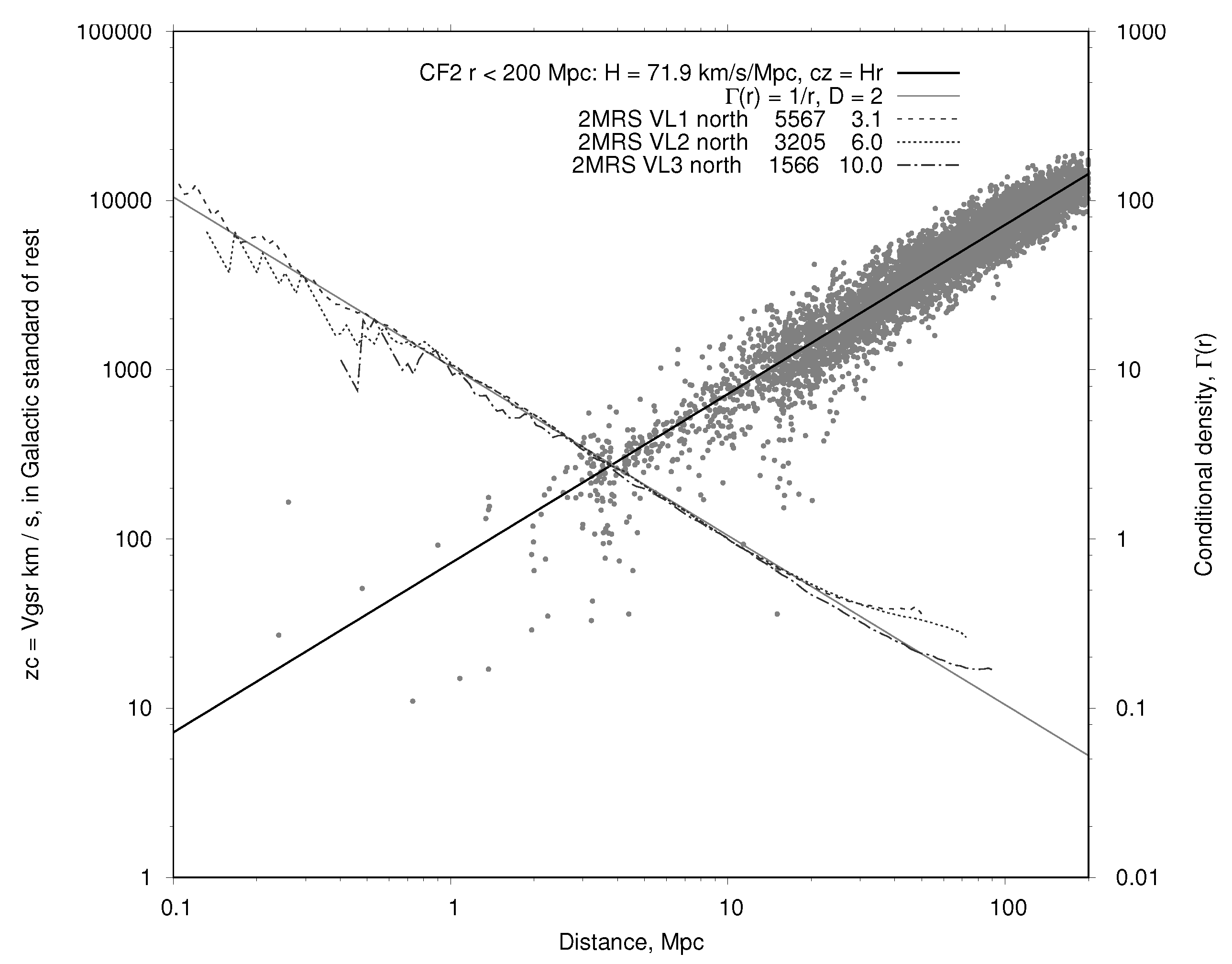
In addition, there are number of observational and conceptual difficulties of LCDM scenario, which discussed in the contemporary literature. Among them, the discovery of strong inhomogeneous galaxy distribution and galaxy flows in the Local Universe, which include such super-large structures as Great Wall, Sloan Wall, South Pole Wall, and others, with sizes up to 400 Mpc Pomarede et al., 2020 [48], Tully et al., 2019 [49], Hoffman et al., 2017 [50], and Tully et al., 2014 [51]. The size 400 Mpc is much more than the 120 Mpc of the baryon acoustic oscillations, where galaxy correlation function of the standard LCDM model must crosses zero level. Complex walls-filament-void structures was discovered by means of distance measurements independent on redshifts in real space for CosmicFlows-2 catalog (Courtois et al., 2013 [52]) and power-law correlation function in redshift space for 2MRS catalog (Tekhanovich & Baryshev 2016 [53]). Additionally, such problems are discussed: the cold dark matter crisis on galactic and sub-galactic scales (Kroupa 2012 [54]); the LCDM crisis at super-large scales (Sylos Labini 2011 [55], Clowes et al., 2013 [56], Horvath et al., 2015 [57]; Shirokov et al., 2016 [58]), existence at high redshifts the old galaxies and the supermassive quasars [59,60,61].
1.1.4. Conceptual Problems of the Gravity Physics
Direct detection (localization) of the gravitational waves by LIGO-Virgo antennas raises the conceptual problem of the GW energy localization in geometrical gravity theory. For the GRT, it is a consequence of the equivalence principle in the metric gravity theories: “...This corresponds completely to the fact that by a suitable choice of coordinates, we can ’annihilate’ the gravitational field in a given volume element, in which case, from what has been said, the pseudotensor also vanishes in this volume element” [27] (§101, p. 307). Note that there is no such problem in electrodynamics and Feynman’s quantum-field gravitation theory, where the field energy-momentum tensor exists and GW energy density in classical limit is well-defined in each point of the Minkowski space.
Conceptual obstacles of GRT, which are directly related to these observations, include well-known “energy-momentum pseudo-tensor” and “horizon” problems. The energy localization problem is that, within GRT, there is no tensor characteristics of the energy-momentum for the gravity field [26,27,28,65,66,67,68]. Landau & Lifshitz 1971 [27] called this quantity pseudo-tensor of energy-momentum and noted that covariant divergence of the total energy-momentum tensor (right side of the Einstein’s field equations Equation (22)) does not express the energy-momentum conservation for matter plus gravity field. The “pseudo-tensor”(meaning non-tensor) character of the gravitational energy-momentum in GRT has been discussed from time-to-time for a century (see a review Baryshev 2008a [65]), causing surprises for each new generation of physicists. However, rejecting the Minkowski space inevitably leads (according to Noether theorem) to deep difficulties with the definition and conservation of the energy-momentum for the gravitational field (see Section 1.3 and Section 2.5).
There are several paradoxes that are related to the concept of black hole horizon, which were emphasized by Einstein 1939 [69]. The information paradox was recently discussed by Hawking 2014 [70], 2015 [71], ’t Hooft 2015 [72], and the incompatibility of classical and quantum concepts of the BH horizon was considered by Chowdhury & Krauss 2014 [73]. The infinite time formation of the classical BH event horizon (in the distant observer’s coordinates) and finite time of BH quantum evaporation means that a BH should evaporate before its formation [73]. Stephen Hawking claimed in [70] that “There would be no event horizons and no firewalls. The absence of event horizons mean that there are no black holes - in the sense of regimes from which light can’t escape to infinity”. Although there is no escape from a black hole in classical theory, but, in quantum theory, energy and information can escape from a black hole. It means that an explanation of the gravity physics requires a theory that successfully merges gravity with the quantum fields of other fundamental forces of nature (actually this is the goal of the field gravitation theory, as we discussed below).
The theory of internal structure of the neutron stars is based on the Tolman–Oppenheimer–Volkov GRT equation of hydrostatic equilibrium for the high-density equation of state. Importantly, first radius-mass measurements of several neutron stars, discovered that there is no reasonable equations of state, which is able to describe the observed parameters of the pulsars, e.g., millisecond pulsar PSR J0030+0451 observed by NICER (Miller et al., 2019 [74]). Additionally, difficulties arise for coalescence of two neutron stars in the event GW170817/GRB170817A giving the resulting mass (2.73–3.07) Abbott et al., 2020 [75].
Additional conceptual problem of the BH physics arises when one considers the process of BH formation from coalesces of two neutron stars or two black holes. The point is that the any binary system of relativistic compact objects has finite binding energy, equals the work against the gravity force needed for destruction of the binary system. However, after the coalescence to one black hole, we get at the classical level the ”infinite binding energy”, because of impossibility to destroy the BH.
For cosmological solutions of GRT equations, there are several conceptual questions discussed in the literature: the Newtonian character of the exact Friedmann equation (Baryshev 2008c [76], 2015 [77]); violation of the energy-momentum conservation within any comoving local volume (Harrison 1995 [78], Baryshev 2008c [76], 2015 [77]); violation of the velocity of light by space expansion velocity for galaxies observed at high redshifts (Harrison 1993 [79], 2000 [80], Baryshev & Teerikorpi 2012 [8] Baryshev 2015 [77]).
So all, mentioned above, recently discussed the observational and theoretical problems of gravitation theory and cosmology point to need for reanalysis of alternative possibilities for construction of the theory of gravitational interaction.
1.2. The Quest for Unification of of the Gravity with Other Fundamental Forces
The success of the Standard Model of electromagnetic, weak, and strong interactions was achieved on the way of unification of the fundamental physical forces in the frame of the quantum field theory (QFT). Now, it has reached a respectable status as an accurate and well-studied description of sub-atomic forces and particles, though difficult conceptual and technical problems remain to be solved (Bogolubov & Shirkov 1993 [81]; Wilczek 1999 [82], 2015a [83], 2015b [84]; Blagojevich 1999 [85]; Pavsic 2002 [86]; ’t Hooft 2004 [87]; Maggiore 2005 [88]; and, “Approaches to Fundamental Physics” 2007 [89]).
Especially important that the unification of gravitational interaction with general quantum physics includes all fundamental principles of modern quantum theory, such as particle-wave duality, quantum uncertainty, amplitude probability for exchange by energy quanta, and, in particular, recently studied irreversibility, non-locality, and quantum entanglement (Kadomtsev 2003 [90], Rauch et al., 2018 [91], Erhard, Krenn & Zeilinger 2020 [92]).
1.2.1. Future Unified Theory
It is expected that future “Core Theory” of physics will unify all fundamental forces (electromagnetic, weak, strong and gravitation) and also deliver unification of forces (bosons) and substances (fermions) via transformations of supersymmetry (Wilczek 2012, 2015a [83,93]).
There is an important obstacle for the unification of fundamental forces with the geometrical gravitation theory (general relativity theory—GRT): the conceptual basis of GRT is principally different from the Standard Model (Ehlers 2007 [66]; Approaches to Fundamental Physics 2007 [89]). Gravity in the frame of GRT is not a force (de Sitter 1916 [94]) and has no generally covariant EMT, so quantization is applied to the curved Riemannian space-time (Rovelli 2004 [89,95]). However the concept of gravitation energy quanta cannot be properly (tensorial) defined in a theory, where the energy of gravitational field is not localized (Ehlers 2007 [66]).
The QFT reconciled Quantum Mechanics with the Relativistic Field Theory by construction of interacting substances via material fields that does obey the laws of Lorentz invariance, gauge invariance, and causality. The concept of a field energy has crucial meaning in the QFT, because the energy in a quantized field comes in quantized energy packages, which, in all respects, behave like elementary particles. The association of forces (or, more generally, interactions) with exchange of particles is a general feature of quantum field theory [89]. Electric and magnetic forces between charged particles are explained as due to one particle acting as a source for electric and magnetic fields, which then influence others. With the correspondence of fields and particles, as it arises in quantum field theory, Maxwell’s ED corresponds to the existence of photons, and the generation of forces by intermediary fields via the exchange of real and virtual photons.
1.2.2. Quantum Electrodynamics as the Paradigmatic Theory
The first step for constructing quantum electrodynamics (QED) is to develop the classical electrodynamics (ED)—the relativistic classical vector field (). In this paper, the ED theory will be used as a primary example for preparation of the classical part of the QFT. Accordingly, below, I emphasize the crucial points of ED (Landau & Lifshitz 1971 [27]), 3 which will be compared with geometrical and field gravitation theories. The second step is to unite the relativistic classical field with quantum mechanical principles.
Classical electrodynamics. As the basic principles of ED one may consider following items:
- the inertial reference frames;
- the flat Minkowski space-time;
- the relativistic vector field ;
- the Least (Stationary) Action Principle;
- the conservation of charges;
- the gauge invariance principle;
- the localizable positive energy density () of the field.
The action S for the system, containing electromagnetic field with charged particles, must consist of three parts:
The notations (f), (int), and (m) refer to the actions for the electromagnetic field, the interaction, and the particles. The physical dimension of each part of the action is
meaning that the definition of energy density of the field must exist within the conceptual bases of the principle of stationary action, -four-current, -four-potential, and -electromagnetic field tensor
From the Least Action Principle () by means of the variation of four-potentials for the case of fixed sources we get field equations with conserved sources
Following Schwinger’s ”source theory” [96,97] in ED the electromagnetic field source is 4-current , which together with the Lorentz invariant law of charge conservation (scalar restriction ) excludes the scalar source of the four-vector field, i.e., the scalar photons. In fact the logic of spin 0 particle exclusion is following:
The left side of the field equations Equation (3) allows for the gauge invariance in the form:
which allows for it to use the Lorentz gauge condition
and the final field equations has ordinary wave equation form
The gauge invariance Equation (5) is consistent with the conservation of the source of the field Equation (3) and with the deleting of the “scalar” photons. Indeed, the four-vector field (four components) can be decomposed into (3 + 1) components [98,99]. Four-potential has four independent components, which correspond to one spin-1 () and one spin-0 () particles, then current conservation law allows for excluding the source of the spin 0 particles, so only photon with spin 1 is real:
The canonical energy-momentum tensor (EMT) of the electromagnetic field, after symmetrization, has the form:
which has following important features:
- -symmetry condition;
- - localizable field energy density, positive for both static and wave field, corresponding to the positive photon energy ;
- -trace of the EMT is zero; for mass-less particles (photons);
- the EMT from action S is defined not uniquely; and,
- the EMT is gauge invariant.
The localization and positiveness of the energy density of the electromagnetic field means that the 00-component of the energy-momentum tensor is defined for any point of the Minkowski space-time and it can be transformed (localized) in the kinetic energy of charged particles (e.g., detection of an electromagnetic wave).
Considering in action S variation the trajectory of a moving charge particle for the case of the fixed four-potential gives the four-equations of motion for charged particle:
or in 3-d form it gives the Lorentz force () and its work ():
and
Thus, in ED, the fundamental role plays the concept of force, work produced by force, positive energy density of the field, and its localization.
Quantum extension of electrodynamics. Adding to ED the quantum physical requirements— the uncertainty principle, probability amplitudes, the principle of superposition, quanta of the field energy as mediators of force, and others, the quantum electrodynamics (QED) was constructed in the frame of QFT and then unified into electro-weak theory and grand unified theory. The canonical quantization and Feynman’s functional integral quantum field theory are presented in general textbooks on QFT (e.g., Bogolubov & Shirkov 1982 [81], Ryder 1984 [100], Sadovskii 2019 [101]).
The QED uses the concept of “force-mediating quantum particles” for describing the electromagnetic force. The virtual-particle description of static force explains the inverse-square behavior of the Coulomb law and predict the repulsive force between the charges with the same signs.
In the path integral formulation of the QED, from the Lagrangians in action Equation (1), while taking into account the field Equation (7), together with the Lorentz invariant law of current conservation (scalar restriction ), one can get the amplitude of particles exchange in the form , where the photon propagator is .
The quantum current-current interaction amplitude, in the case of exchange of one particle having four-momentum , can be written in the form (Feynman et al., 1995 [17]):
where the frequency dependent part of the amplitude Equation (13) gives electromagnetic radiation.
The instantaneous part of the amplitude Equation (13) corresponds to the Poisson equation for electrostatic potential
which, now, has the quantum nature. Thus, the Coulomb law for the electrostatic force is explained through the probability amplitude, which gives the energy of interaction
and corresponds to the repulsion for similar signs and to the attraction of opposite sings of charges.
Note that, in the case of massive photon (Proca mass term), the propagator can be written in the form ). As a result, the exchange amplitude between two conserved sources is the same in the limit , no matter whether the vector field is intrinsically massive (propagates three degrees of freedom) or if it is massless (propagates two degrees of freedom). Therefore, it is impossible to probe the difference between an exactly massive vector field and a massive one with arbitrarily small mass [6].
1.3. Einstein’s Geometrical and Feynman’s Quantum-Field Gravitation Physics
1.3.1. Two Ways in Gravity Physics
Since the beginning of the 20th century two really alternative approaches were put forward for the description of the gravitational interaction in theoretical physics.
The first approach is the geometrical Einstein’s general relativity theory (GRT), which is based on the geometrical concept of curved Riemannian (actually pseudo-Riemannian) space and rejects the ordinary physical concept of force in application to gravitation. GRT was founded by Einstein 1915 [13]; 1916a [102]; and, Hilbert 1915 [14], and it gives an example of geometrical way in construction of gravity theory. GRT operates with such concepts as metric tensor , geodesics, curvature, equivalence of the free fall to the inertial motion. Wheeler termed this approach geometrodynamics, underlining the fact that geometry is not a passive background but becomes a dynamical physical entity that may be deformed, stretched and even spread in the form of gravitational waves. Geometrical gravity treats the gravitational interaction as the curvature of space and it has a singular position among other physical interactions, which are based on the physical concept of the force caused by the exchange of the field quanta in Minkowski space.
During one hundred years, GRT was developed and successfully applied to many gravity phenomena in the Solar System, galactic, and extragalactic astronomy (Debono & Smoot 2016 [5], Will 2014 [15]; Straumann 2013 [67]; Kopeikin, Efroimsky, Kaplan 2011 [103]; Schuts 2009 [104]; Brumberg 1991 [105]; Misner, Thorne & Wheeler 1973 [28]; Weinberg 1972 [106], 2008 [107]; Landau & Lifshitz 1971 [27]; and, Zeldovich & Novikov 1984 [108]). However, general relativity is not a quantum theory and many attempts to construct geometrical quantum gravity theory have not yet brought generally accepted convincing solution of the “Quantum theory’s last challenge” (Amelino-Camelia 2000 [109]; Approaches to Fundamental Physics 2007 [89]; Wilczek 2015a,b [83,84]).
The second approach for alternative understanding gravity was already suggested by Poincaré, who considered gravitation as a fundamental force in relativistic space-time. As early as 1905, Poincaré in his work “On the dynamics of the electron” put forward an idea about relativistic theory for all physical interactions, including gravity, in flat 4-d space-time (now called Minkowski space). He pointed out that analogously to electrodynamics, gravitation should propagate with the velocity of light, and there should exist mediators of the interaction—gravitational waves, l’ onde gravifique, as he called them (Poincaré 1905 [110]; 1906 [111]). A few years later in his lecture on “New concepts of matter” Poincaré wrote about inclusion Planck’s discovery of the quantum nature of electromagnetic radiation into the framework of future physics for all fundamental interactions. Poincaré, thus, could be rightfully regarded as the visionary of that approach to gravity that describes gravitation as the relativistic quantum field in Minkowski space.
According to Feynman’s Lectures on Gravitation (1971 [16], 1995 [17]) (Caltech lectures in 1962–1963) the field gravitation theory (FGT) must be relativistic and quantum, which is described by symmetric second rank tensor field in Minkowski spacetime. Accordingly, as in the theory of electromagnetic interaction we have electrodynamics (ED) and quantum electrodynamics (QED), in the case of FGT we should consider “gravidynamics” (GD) and quantum-field gravitation theory (QFGT)—“quantum gravidynamics” (QGD). Within QFGT, as in QED, general concepts of force and localizable positive field energy density naturally exist, and QFGT should be included in the list of the field theories of fundamental physical interactions.
Because of the great success of general relativity in explanation of existing experimental and observational facts in gravity physics, the field gravitation theory up to now has been outside general attention. However the field approach to gravitation was partly developed by number of famous physicists, among them Birkhoff 1944 [112]; Moshinsky 1950 [113]; Thirring 1961 [18]; and, Kalman 1961 [114]. Attempts for a field-theoretical description of the gravitational field quantization were made by Bronstein 1936 [115]; Fierz & Pauli 1939 [116]; Ivanenko & Sokolov 1947 [117]; Gupta 1952a,b [118,119]; Feynman 1963 [120]; 1971 [16]; Weinberg 1965 [121]; Zakharov 1965 [122]; Ogievetsky & Polubarinov 1965 [123], Blagojevich 1999 [85], Maggiore 2008 [26]; and, others.
It is important to note that in Feynman’s Lectures on Gravitation the gravitational field is initially described as the reducible symmetric second rang tensor , which can be presented as a direct sum of three irreducible representations of the Poincare group: four-tensor (traceless), four-vector, and four-scalar (5 + 4 + 1 = 10 components). Gauge invariance (and corresponding EMT conservation) only excludes four components (four-vector) and, hence, leaves direct sum of two irreducible representations: spin-2 and spin-0 parts (i.e., six independent components). The irreducible spin-2 representation describes the attractive force and Feynman (as many other authors of the spin-2 derivations of GRT equations) tried to construct gravitation theory based on the spin-2 field only, so excluding spin-0 field.
The fundamental role of the 4-scalar spin-0 component (the trace ), which is the second irreducible part of the gauged total reducible symmetric tensor potential , was found and developed by Sokolov and Baryshev [19,20,65,124,125,126,127,128,129]. Intriguingly this irreducible intrinsic 4-scalar field corresponds to the repulsive dynamical field, which in the sum with the pure spin-2 field gives the Newtonian gravity force and also all classical relativistic gravity effects. As a result, a consistent field gravity theory (FGT) has been developed, where the central role belongs to the inertial frames, Minkowski space and localizable positive energy of the gravitational field, including its scalar part. Although many important questions are waiting for further work.
The relation between GRT and FGT was discussed in the literature with a very wide spectrum of opinions. There is a statement about the identity of the field gravity to the general relativity, so they are “just different languages” leading to the same experimental predictions, and after “repairing” the spin-2 approach becomes GRT (Misner, Thorne, Wheeler 1973 [28]). Additionally, there is the claim, that the metric gravity theory is the only possible way to construct the correct gravitation theory (Misner, Thorne, Wheeler 1973 [28]; Straumann 2013 [67]). Let us consider the real state of art of the problem.
1.3.2. Special Features of the Geometrical Approach
Within a geometrical approach, the gravitational interaction is described as a curvature of space-time with the metric . A deep analysis of the GRT basic principles was done by Ehlers 2007 [66] and Straumann 2013 [67]. Here, I emphasize that GRT is a non-quantum relativistic theory of the gravitational interaction and based on the following fundamental concepts:
- the non-inertial reference frames;
- the equivalence principle and geometrization of gravity;
- the curved Riemannian space-time with metric ;
- the geodesic motion of matter and light;
- the general covariance; and,
- the geometrical extension of Stationary Action Principle.
Note that the equivalence principle (EP) played an important role in the history of the general relativity formulation. EP has many forms—from non-relativistic to philosophical, which are not equivalent and difficult to test. Actually in experiment one tests the universality of the free fall, which is expected to be independent on the structure and motion of a test body (also known as the effacing principle [67,103]). Another form of the EP is the geometrization principle, i.e., the metric representation of gravitational potentials and geodesic motion in Riemannian space, which now is considered to be the primary initial assumption of the geometrical approach (Ehlers 2007 [66]). However, the geometrical quantum gravity approach predicts violation of the EP and Lorentz invariance (Amelino-Camelia et al., 2005 [130]; Bertolami et al., 2006 [131]).
On the bases of its initial principles, general relativity was developed and successfully applied to the number of experiments and observations in the weak gravity conditions ([15,67]). Strong gravity GR predictions, like gravitational collapse to singularity, black hole existence, and global space expansion, may only be observed within astrophysical conditions, where the interpretation of the data allows for different possibilities due to specific passive character of the astronomical observations and the dominance of distortion and selection effects which influence real astronomical data. So, in spite of many claims about proved existence of black holes and space expansion, up to now there is no direct experimental/observational proof of the GRT strong gravity effects, which are still hypothetical models for the observed astrophysical phenomena (see discussion in Section 4 and Section 5).
In conditions of the weak gravity general relativity is a well verified theory. It has passed all available tests in the Solar System and binary pulsars. Nevertheless, more accurate and conceptually new tests in the weak-field regime are still needed, as well as tests of strong-gravity effects (Fabian 2015 [37]; Wilkins 2015 [38]; Baryshev 2015 [77]; Sokolov 2015 [128]; Will 2014 [15]; Doeleman 2009 [31]; Baryshev 2008b [132]; and, Bertolami et al., 2006 [131]).
1.3.3. Problem of the Gravitational Field Energy-Momentum in GRT
The most puzzling feature of general relativity is the absence of the tensor character of the “energy-momentum tensor” for the gravity “field”. This was clearly exposed already by Einstein 1918 [133,134]; Schrödinger 1918 [135]; Bauer 1918 [136], and more recently discussed by Landau & Lifshitz 1971 [27]; Misner, Thorne & Wheeler 1973 [28]; Logunov & Folomeshkin 1977 [137]; Strauman 2000 [138], 2013 [67]; Pitts & Schieve 2001 [139]; Xulu 2003 [140]; Ehlers 2007 [66]; and, Baryshev 2008a [65].
The problem of the energy of the gravity field in general relativity has a long history, it was, in fact, born together with Einstein’s equations. Hilbert 1917 [141] was the first who noted that “I contended … in general relativity … no equations of energy … corresponding to those in orthogonally invariant theories”. Here, “orthogonal invariance” refers to theories in the flat Minkowski space. Emmy Noether 1918 [142], a pupil of Hilbert, proved that the symmetry of Minkowski space is the cause of the conservation of the energy-momentum tensor of all physical fields. Many results of modern relativistic quantum field theory are based on this theorem. Accordingly, the “prior geometry” of the Minkowski space in the field theories has the advantage of guarantee the tensor character of the energy-momentum, its localization and its conservation for the fields. However, in GRT, there is no global Minkowski space, so there is no EMT of the gravitation field and its conservation.
In fact, Einstein & Grossmann 1913 [143] came close to Noether’s result when they wrote: “remarkably the conservation laws allow one to give a physical definition of the straight line, though, in our theory, there is no object or process modeling the straight line, like a light beam in ordinary relativity theory”. In other words, they stated that the existence of conservation laws implies the flat Minkowski geometry. In the same article, Einstein & Grossmann also emphasized that the gravity field must have an energy-momentum tensor as all other physical fields. However, in the final version of general relativity, Einstein rejected this requirement in order to have a generally covariant gravity theory with no prior Minkowski geometry.
Schrodinger 1918 [135] showed that the mathematical object suggested by Einstein in his final general relativity for describing the energy-momentum of the gravity field may be made vanish by a coordinate transformation for the Schwarzschild solution if that solution is transformed to Cartesian coordinates. Bauer 1918 [136] pointed out that Einstein’s energy-momentum object, when calculated for a flat space-time, but in a curvilinear system of coordinates, leads to a nonzero result. In other words, can be zero when it should not be, and it can be nonzero when it should (this also emphasized by Landau & Lifshitz 1971 [27] (§101, p. 307)).
Einstein 1918a [133] replied that already Nordstrom informed him about this problem with . Einstein noted that in his theory is not a tensor and also it is not symmetric. He also withdrew his previous demand of the necessity to have an energy-momentum tensor: “there may very well be gravitational fields without stress and energy density”.
The “pseudo-tensor” (meaning “non-tensor”) character of the gravity field in GR has simple mathematical cause. As emphasized by Landau & Lifshitz 1971 [27] (§101, p. 304) due to Bianchi identity the covariant divergence of the right part of Einstein’s equation (which is the EMT of matter ) is equal to zero, i.e., . However, for conserved quantity one should have the ordinary partial divergence: . Accordingly, Landau & Lifshitz suggested to consider pseudo-tensor (non-tensor) of energy-momentum of gravitational field which should be added to the EMT of matter and allow to fulfill the needed equation .
There are many different expressions for pseudo-tensors, but the problem of coordinate dependent (non-physical) definition of the gravity energy-momentum still exists at fundamental level—gravitational field is not a matter within GRT. This also demonstrates that rejecting the Minkowski space inevitably leads to deep difficulties with the definition and conservation of the energy-momentum for the gravity field.
1.3.4. Attempts to Resolve the Gravitational Energy-Momentum Problem in Geometrical Approach
The main question of the gravity physics is the role of the global Minkowski space in the gravitation theory. Within the geometrical approach Minkowski space is a tangent space at each point of curved space (the local Lorentz invariance). The field approach utilizes the global Minkowski space to describe all four fundamental physical interactions as material fields in space.
According to Noether’s theorem in the relativistic field theory, the conservation of the energy-momentum relates to the flat global Minkowski space. However, in general relativity there are no conservation laws for the energy-momentum of the matter plus gravity field, just because of the absence of the global Minkowski space. The energy problem has deep roots in the geometrical approach, which uses curved space and non-inertial reference frames, while the field approach based on the Minkowski space with inertial reference frames naturally contains local EMT for the gravity field.
Note that, in GRT, there is a suggestion for consideration of observable gravity effects without using the general covariant concept of the gravitational energy (Strauman 2013 [67]; Maggiore 2008 [26]). Also in GRT there are attempts to construct of a “quasi-local” energy-momentum and angular momentum to save the physical concept of the energy for the gravity “field” (Szabados 2009 [144]). There are also several suggestions how to overcome the energy-momentum problem by a modification of general relativity, or by postulating additional constraints on the metric of the Riemannian space, or by introducing Minkowski and Riemannian metrics together. This has led to different “field-geometrical” gravity theories (which actually belong to metric gravity theories) having different equations and predictions (e.g., Logunov 2002 [145]; Logunov & Mestvirishvili 1989 [146], 2001 [147]; Yilmaz 1992 [148]; Babak & Grishchuk 2000 [149]; Pitts & Schieve 2001 [139]; and, Xulu 2003 [140]).
All these theories are geometrical (they use geometrization principle) and they predict some differences with GRT only in the case of the strong gravity field, which is not directly observed yet. However, as we shall show below, the results of the consistent Poincare–Feynman field approach has led to predictions that differ from GRT, even in the weak field conditions, which, in principle, can be tested by experiments in the Earth laboratories and by observations while using terrestrial and space observatories.
1.3.5. Special Features of the Feynman Approach
Feynman discussed the strategy of the QFGT and suggested constructing “theory of gravitation as the 31st field to be discovered” [17] (p. 15). He analyzed basic principles of the QFGT and emphasized, that “geometrical interpretation is not really necessary or essential for physics” [17] (p. 113).
Accordingly, the natural relativistic quantum field approach to gravitational interaction should be developed on the way where other fundamental interactions already have been constructed. Feynman emphasized that the “world cannot be one-half quantum and one-half classical” and “it should be impossible to destroy the quantum nature of fields” [17] (p. 12).
Modern physics deals with four presently known fundamental interactions: the electromagnetic, the weak, the strong, and the gravitational. The first three interactions are described by using Lagrangian formalism of the relativistic quantum field theory in Minkowski space. The QFGT theory also should be based on the same Lagrangian concepts, also including specific scalar-tensor character of the gravitational field:
- the inertial reference frames;
- the flat Minkowski space-time wih metric ;
- the reducible symmetric tensor potentials with trace ;
- the universality of gravitational interaction;
- the Stationary Action Principle (Lagrangian formalism);
- the conservation law of energy-momentum tensor;
- the gauge invariance principle;
- the localizable positive energy density of the gravitational field;
- the gravitational field energy quanta as mediators of the gravity force; and
- the uncertainty principle and other quantum postulates.
In Section 3, we discuss how to construct the consistent Poincare–Feynman field gravity theory based on these initial principles. The energy of the gravitational field should play the central role in a reasonable theory of gravitational interaction. Feynman’s notorious words in a letter to his wife “Remind me not to come to any more gravity conferences” ([17] Foreword p. xxvii) are related to this very issue, he did not wish to discuss the question of whether there is energy of the gravitational field. For him, gravitons were particles carrying the energy-momentum of the field: “the situation is exactly analogous to electrodynamics—and in the quantum interpretation, every radiated graviton carries away an amount of energy ” [17] (p. 220).
Nowadays, when the Nobel Prize in Physics (1993) was given for the discovery of the binary pulsar PSR 1913+16, which is emitting positive energy of gravitational radiation, and the Advanced LIGO gw-antennas have detected the gravitational waves (i.e., have localized positive gw-energy), it is clear that Feynman was right when insisting on the necessity to have proper concept of the energy density of the gravitational field.
1.3.6. Why Is QFGT Principally Different from GRT?
The history of the field gravity approach is characterized by many controversial opinions and misleading claims (a review in [150]). From time to time at a gravity conference, a physicist appeared who announced that he ultimately had just derived the full non-linear Einstein’s equations from the spin 2 field approach and he will demonstrate it at the next conference. However, at the next conference the situation was repeated.
The incompatibility of geometrical (GRT) and quantum field (FGT) approaches exists on the level of the adopted initial conceptual principles (Ehlers 2007 [66]), which we have considered above. The most important difference is the geometrization principle in GRT (gravitational potentials are described by the metric tensor of the Riemannian space), while in FGT gravitational potential is the material field in Minkowski space with metric . Accoridngly, the gauge transformation in FGT is related to potentials in a fixed inertial frame, while in GRT the gauge transformation is the change of coordinates. In the field gravity approach there is usual localizable energy-momentum tensor (EMT) of the gravitation field, while, in the geometrical approach, there is no tensor quantity for the gravitational energy-momentum (problem of pseudo-tensor).
In the frame of QFGT, the symmetric tensor potential actually corresponds to the reducible representation of the Lorentz group, which can be decomposed to the direct sum of three irreducible representations: traceless four-tensor, four-vector, and four-scalar (5 + 4 + 1 = 10 components). 4 After the four gauge conditions, one excludes four-vector field (spin-1 and spin-0 particles: four components), so the initial reducible tensor field will only contain two irreducible representations corresponding to spin-2 and spin-0 particles ( components). The gauge freedom is also consistent with the four conditions from conservation of the field source, so that the two types of particles have corresponding parts of the source, and the final field equations describe two real dynamical fields.
Accordingly, according to Wigner’s theorem [151], the QFGT is the scalar-tensor field gravitation theory. Note that the intrinsic scalar part of the symmetric tensor field (trace ) is an observable part of the classical gravity experiments (see Section 3). The most radical difference of QFGT from GRT is that the field approach works with the two parts of the gravity physics - the traceless spin-2 attraction field and the intrinsic scalar spin-0 repulsion field (the trace of the tensor potential). This fact demonstrates the principal incompatibility of FGT and GRT, though there is common region of applicability of geometrical and field approaches (coincident predictions for classical relativistic gravity effects in the weak field regime).
However, up to now, there are attempts to “prove of identity” of GRT and FGT approaches by using two opposite ways, so called “top-down” and “down-top” argumentations.
The top-down approach starts from the “top” full non-linear Einstein equations and goes to the “down”—linear weak field approximation, where the metric tensor of the Riemannian space only slightly differs from the metric tensor of the Minkowski space. Accordingly, metric tensor is defined by the relation (first suggested by Einstein 1916b [152]):
where the quantities , and the rigorous identities must be fulfilled for the metric tensor of any Riemannian space:
In this weak field approximation, the Einstein’s field equations are equivalent to the field equations of the relativistic symmetric second rank tensor field in Minkowski space with metric . Working with the linear approximation of the Einstein’s equations, one usually uses the convention that indices are rased and lowered by the flat metric . However strictly speaking in the frame of the geometrical approach such procedure is “illegal”, because it violates the general covariance principle ( and are not tensors of the initial curved space). For the rasing and lowering indices, one should use the sum (Equation (16)), which must obey the strict identities (Equation (17)). As Schuts 2009 [104] (p. 199) emphasized: “Thus —is not the deviation of from flatness”.
Subsequently, in fact using the field-theoretical approach in Minkowski space, one can calculate the retarded potentials and emission of gravitational waves, which corresponds to the field quanta—spin 2 massless particles, together with additional condition (TT-gauge): (Bronstein 1936 [115]; Fierz & Pauli 1939 [116]; Ivanenko & Sokolov 1947 [117]; Gupta 1952a,b [118,119]; Feynman 1963 [120]; Zakharov 1965 [122]; Maggiore 2008 [26]; and, Straumann 2013 [67]).
It is clear that such “derivation” does not prove an “identity” of GRT and FGT. The Equation (16) means that the geometrization principle is given up because quantities and are not tensors of the Riemannian space, but they are tensors only for the Minkowski space. Here one meets the point where the initial principles of general relativity are replaced by the initial principles of the field gravitation theory.
The down-top approach starts from the “down” linear equations for material symmetric tensor potentials in Minkowski space and goes to a derivation of the “top” nonlinear Einstein’s equations for the “effective metric tensor” of the Riemannian space (Weinberg 1965 [121]), Ogievetsky & Polubarinov 1965 [123]; Deser 1970 [153]; Feynman 1971 [16]; Feynman 1995 [17]; Misner, Thorne, Wheeler 1973 [28]). However, there are fundamental obstacles of such transformation of material tensor field of Minkowski space into non-material metric .
First, the strict properties of the metric tensor of the Riemannian space Equation (17) and the general tensor rules for physical quantities in Minkowski space demand that for the sum of two quantities and , one gets the following expressions (correct to the first order of and ):
As we see from Equation (18), there is essential difference between the geometrical approach and the field approach. The consistent field approach demands that the sum of two tensors must be a tensor of Minkowski space. Indeed the trace of the “effective metric” is a function of space-time , due to the trace of the gravitational potentials , i.e., . Hence, tensor can not be the metric tensor of a Riemannian space and, in the geometrical approach, the scalar part of the symmetric tensor field is lost.
From Equation (18), we see that a tensor of Riemannian space is presented by the sum of two non-tensor quantities and . For example, in the third identity of Equation (18) the components strictly speaking must be zero . The different signs of the quantities for covariant and contravariant components of the metric tensor are caused by the exact identity valid for the trace of the metric tensor of any Riemannian four-space. In the frame of FGT, the tensor cannot be a metric tensor of a Riemannian space (the ), so the field approach cannot be identical to a metric gravity theory.
Feynman, in his lectures on gravitation, also tried to derive the full nonlinear Einstein’s Lagrangian by iterating the Lagrangian of the spin 2 field. Misner, Thorne & Wheeler [28] (Chapter 7, p. 178) wrote that “tensor theory in flat spacetime is internally inconsistent; when repaired, it becomes general relativity”. They refereed to papers by Feynman [120], Weinberg [121], and Deser [153] on a “field” derivation of Einstein’s equations. However, this “repairing” means replacing the field-theoretical approach in Minkowski space by the geometrization principle of the geometrical approach.
Note that, in all such derivations as the first step, they get the “spin-2” field equations (i.e., FGT linear approximation including the scalar part), and they are equivalent to Einstein’s equations in the linear approximation (which also include the scalar part—the trace ). To perform the next step to obtain nonlinear equations, one needs to fix the EMT of the gravitational field (which is the basic concept in the consistent field approach). At this step, one should use the physical concept of the gravitational field EMT, which is not uniquely defined by Lagrangian formalism and it must include additional physically necessary properties, such as localizability, positiveness for both static and variable field and zero trace (for massless gravitons). However, these crucial features of the gravitational field disappear in the “top” non-linear Einstein’s equations (generating the problem of non-localizability of the energy-momentum pseudotensor in GRT). Just this crucial step is still a controversial subject. This is why many physicists feel a tenuity of such derivation and try to get his personal derivation of the geometry from field approach, although, as we demonstrated above, it is impossible on the conceptual level.
1.3.7. Conceptual Tensions between Quantum Mechanics and General Relativity
According to Wigner’s theorem [151], quantum physical particles are the irreducible unitary representations of the Poincare (inhomogeneous Lorentz) group and, hence, demand the existence of the total symmetry of the Minkowski spacetime. Conceptual tensions between geometrical and quantum-field approaches to gravitation theory were noted by some physicists (Wigner 1997 [154]; Feynman 1995 [17]; Amelino-Camelia 2000 [109]; Chiao 2003 [155]; and, Ehlers 2007 [66]). The most pressing problem in present-day theoretical physics is how to unify quantum theory with gravitation, i.e., “quantum gravity problem”. The standard scheme of quantization applied to general relativity gives a theory that is not renormalizable (i.e., leads to infinities in physical quantities), though, in principle, non-renormalizability is a temporary technical obstacle. Quantization of space-time is now also under construction [89,95], including the string/M theory, canonical/loop quantum gravity, non-commutative geometry, and other [86]. However the difficulties on this way so large that after all attempts there is still no quantum geometrical gravity theory (Amelino-Camelia 2000 [109]; Amelino-Camelia et al., 2005 [130]).
Note that, if in a physical theory, the energy-momentum tensor of the field is not defined, then also the energy of the field quanta can not be defined properly. General relativity is not quantizable in ordinary physical sense because it has no energy-momentum tensor for the gravity field. Additionally, it is important that properly defined energy of the gravity field also excludes an appearance of singularity and horizon (Section 4.2).
Additional inconsistencies of attempts to derive Einstein’s equations from the spin 2 field theory, was noted by Straumann 2000 [138] (p. 16), who pointed out that:
- general relativity having black hole solutions violates the simple topological structure of the Minkowski space of the quantum field theory;
- general relativity has lost the energy-momentum tensor of the gravity field together with the conservation laws, while in the Standard Model the EMT and its conservation is the direct consequences of the global symmetry of the Minkowski space.
Padmanabhan 2004 [156] gave a comprehensive review of all such attempts and demonstrated that all derivations of general relativity from a spin 2 field are based on some additional assumptions that are equivalent to the geometrization of the gravitational interaction.
Indeed, as we noted above, general relativity and field gravity rest on incompatible physical principles, such as non-inertial frames and the Riemann geometry of curved space on the one side, and material tensor field in inertial frames with Minkowski geometry of flat space on the other side. Geometrical approach eliminates the gravity force, as already noted by de Sitter [94]: “Gravitation is thus, properly speaking, not a ’force’ in the new theory”. This however leads to the problem of energy just because the work done by force changes the energy.
Within the quantum-field approach the gravity force is directly defined in an ordinary sense as the fourth interaction and has quantum nature (Feynman [16,17]). The question may be formulated, as following, which is more general description of gravitation: geometry of curved space (so a property of space-time itself) or relativistic quantum field (so a kind of matter) in space?
1.3.8. Astrophysical Tests of the Nature of Gravitational Interaction
The relation between GRT and QFGT is still an open question. Intriguingly, due to different predictions for observations, this question can be answered by means of astrophysical observations and lab experiments, so to test which theory has a wider region of applicability?
In physics, any mathematical theory has restricted region of applicability, i.e., exact mathematical equations and it’s solutions actually have only approximative physical sense. This is why in physics the last word belong to experiments, and especially to the crucial experiments and observations, when rival theories predict different results for certain clearly stated experiment. The geometrical and field approaches are not equivalent experimentally, though the classical relativistic gravity effects in the weak field are identical in both theories. Because of the common region of experimentally tested effects, it is possible that geometrical approach can be an approximation of the true quantum field gravity or vise verse.
Geometrical approach of the classical general relativity predicts such specific objects as singularities, black holes, and expanding space of Friedmann cosmological model.
The consistent field approach predicts that the gravity force has an ordinary quantum nature. Actually, the gravity force is the sum of the attraction (spin-2) and repulsion (spin-0) (as will be shown in Section 3 and Section 4). This prediction of the QFGT theory opens up possibilities for novel type of experiments in gravity physics. Spin-2 plus spin-0 contribution to the gravity force, scalar gravitational waves, the translational motion of rotating bodies, the atmosphere and the magnetic field of the relativistic compact objects in “black hole candidates” are specific effects of the field gravity that may distinguish QFGT from general relativity. In cosmology within the frame of QFGT, there is a possibility of infinite flat static Minkowski space filled by evolving baryonic and non-baryonic matter and having linear Hubble law of cosmological redshift as the global gravitational redshift effect (see Section 5).
It is a remarkable result of our considerations that the choice between two conceptually different gravity theories may be founded on the results of experiments/observations in a physical laboratory. For example, the problem of gravity quantization is directly linked to the choice of the nature of gravitational interaction. Indeed, if gravity is geometrical in nature (a property of curved space), then one should develop methods of space-time quantization [89,95]. However, if gravity is a force that is mediated by gravitons (quanta of the tensor relativistic field), then one should find methods based on the concept of the energy of the gravity field and develops new principles for overcoming the non-renormalizability problem. It will be shown below that future astrophysical observations of the compact relativistic objects, space experiments in the Solar System, and cosmologically relevant observations of the Local and High Redshift Universe may distinguish between these two cardinally different (though having similar predictions within common region of applications) approaches to the theory of gravitational interaction.
2. Einstein’s Geometrical Gravitation Theory
The final mathematical formulation of the main equations of general relativity was done by Einstein [13,102] and derived by Hilbert [14] from geometrical extension of the stationary action principle. It is a mathematically exact non-linear theory without any inner limitations to its physical applications and this is why in GRT singularities and black holes exist. Below, we shortly consider the basic steps in construction GRT and its main predictions for experiments/observations, which we shall compare with corresponding equations and predictions of the QFGT. We use designations as in the textbook by Landau & Lifshitz [27]. The fundamental physical constants are explicitly used because they are important parts of the gravity physics.
2.1. Basic Principles of GRT
2.1.1. The Principle of Geometrization
General relativity is based on the principle of geometrization, which states that all gravitational phenomena can be described by the metric of the Riemannian space (Ehlers 2007 [66]). This means that Einstein’s gravity theory has no “prior geometry”, such as the flat Minkowski space in other fundamental interaction theories. Gravity is not a material field in space, but it is a property of the curved space itself. The role of the gravitational “potential” is played by the metric tensor which determines the four-interval of the corresponding Riemannian space:
A test particle moves along a geodesic line of the Riemannian space.
Note that geodesic motion is a form of the equivalence principle, which actually has many “non-equivalent” formulations like universality of free fall or philosophical equivalence of the inertial reference frames to the reference frames accelerated by homogeneous gravity field. Equivalence principle played an important role when general relativity was born, while, now, the basic principle is the principle of geometrization, having clear physical and mathematical formulation. The most clear and concise presentation of GR is the textbook by Landau & Lifshitz [27]. The most comprehensive description of the geometrical view on gravity is the textbooks Misner, Thorne & Wheeler [28] and Straumann 2013 [67].
2.1.2. The Principle of Least Action
Einstein’s field equations are obtained from the principle of least (stationary) action by the variation of the metric tensor in the action S of the system matter + gravitational field. It is very important to note that instead of the three parts (field-interaction-matter) of the total action in ordinary field theory, in the GRT the total action contains only two parts (there is no interaction Lagrangian), because gravitation is not a matter in GRT (while other fields contain the interaction part , see Equations (1) and (39)). So the GRT action is:
where and are the actions for the matter and gravitational field, is the Lagrangian for the matter, and the Lagrangian for the field is
Here, ℜ is the scalar curvature of the Riemannian space.
2.2. Basic Equations of General Relativity
2.2.1. Einstein’s Field Equations
Variation , with restriction gives from the following field equations:
where is the Ricci tensor. is the energy-momentum tensor (EMT) of the matter, which includes all kinds of material substances, such as particles, fields, radiation, and dark energy, including the vacuum (where is the Einstein’s cosmological constant).
Note that does not contain the energy-momentum tensor of the gravity field itself, because gravitation is not a material field in general relativity (as was discussed in Introduction).
2.2.2. The Equation of Motion of Test Particles
A mathematical consequence of the field Equation (22) is that, due to Bianchi identity, the covariant derivative of the left side equals zero, so for the right side we also have
This continuity equation also gives the equations of motion for a considered matter. 5 It implies the geodesic equation of motion for a test particle:
is the four-velocity of the particle and is the Christoffel symbol.
2.3. The Weak Field Approximation
All of the relativistic gravity effects that have been actually tested by observations, relate to the weak field, where the Newtonian potential . This is why the weak field approximation has an important role in gravity physics.
2.3.1. The Metric Tensor
In the case of a weak gravity field, the metric tensor usually is expressed in the form
As we discussed above, such a presentation of the metric tensor Equation (25) means that a tensor of Riemannian space is presented by the sum of two non-tensor quantities, because and are not tensors of the curved space. e.g., in the third identity of Equation (25) the components must be (though usually the convention is used that and ). The different signs of the quantities for covariant and contravariant components of the metric tensor are caused by the exact identity valid for the trace of the metric tensor of any Riemannian four-space:
As we shall see below, this is an essential difference with the consistent field approach, where the sum of two tensors is a tensor of Minkowski space.
2.3.2. The Field Equations
In the linear GRT approximation, it is assumed that the metric tensor is (Equation (25)) where , so the Einstein’s Equation (22) becomes [26,67]:
The gauge freedom of the Equation (27) allows for one to put four additional conditions on the potentials, in particular a Lorentz invariant gauge—the Hilbert-Lorentz gauge 6 [26,67]:
With the gauge (28), the field equations get the form of the wave equation:
For the important case of a static spherically symmetric weak gravitational field, the solution of these equations gives the metric tensor, expressed in isotropic coordinates:
where is the Newtonian potential. Note that is not a tensor quantity (see Equation (18)).
2.3.3. The Equation of Motion in the Weak Field
The post-Newtonian approximation of the weak field takes all terms of order and into account. PN-geodesic equations are frequently used in relativistic celestial mechanics. The three-acceleration of a test particle in the static spherically symmetric weak gravity field (e.g., a planet around the Sun) is given by equation (Brumberg 1991 [105]; Kopeikin et al., 2011 [103]):
where , , and . An important quantity here is the parameter . It is determined by the choice of the coordinate system: for the Painleve coordinates, for the Schwarzschild coordinates, and for harmonic and isotropic coordinates. Hence orbit of a particle will depend on the chosen coordinates. To avoid this non-physical result it is suggested that observable physical quantities should not depend on the coordinate parameter by taking into account an ad hoc procedure of measuring quantities involved in the orbital motion phenomenon. 7
It should be emphasized that directly from equation of motion (31) follows the dependence of gravitational acceleration from the value and direction of the test particle velocity. Accordingly, this result contradicts that form of the equivalence principle, where one asserts the independence of the free fall on the velocity of a test particles.
2.4. Major Predictions for Experiments/Observations
The number of predictions of general relativity for both weak and strong fields were derived from Einstein’s field equations and the equations of motion. The triumph of GR in physics and astronomy is caused by the experimental and observational confirmation of Einstein’s equations with high accuracy. The application of GR to cosmology will be considered in Section 5.
2.4.1. The Classical Relativistic Gravity Effects in the Weak Field
The classical weak gravity effects have been tested with an accuracy of about % (Will [15]; Kopeikin et al. [103]). Among these experimentally verified effects are:
- universality of free fall for non-rotating bodies,
- the deflection of light by massive bodies,
- gravitational frequency-shift,
- the time delay of light signals,
- the perihelion shift of a planet,
- the Lense–Thirring effect,
- the geodetic precession of a gyroscope, and
- the emission and detection of the quadrupole gravitational waves.
In the next sections, we shall show that all these effects can be explained also within the field gravity approach with the same formulas for the observed quantities; hence, they can not distinct between GRT and QFGT. However, in FGT, there are additional weak gravity effects that can be used as crucial tests for GR and FG theories: e.g., free fall of rotating bodies, attraction, and repulsion components of the gravitational force, and additional scalar gravitational radiation. Recently detected GW signals by Advanced LIGO antennas are also disccussed in Section 4.2.
2.4.2. Strong Gravity Effects in GRT: Schwarzschild Metric
General relativity predictions for the strong gravity considered in many books, which contain many exact solutions of the full non-linear Einstein’s equations (e.g., Landau & Lifshitz [27], Misner, Thorne & Wheeler [28], and Straumann 2013 [67]). Some observable constrains on strong gravity effects was considered by Taylor et al. 1992 [157].
One of the basic exact solution of Einstein’s Equation (22) for any centrally symmetric mass distribution is called the Schwarzschild metric. It has the following form for the four-interval in the Schwarzschild system of coordinates :
In other coordinate systems, this interval has a different form for the singular term. The metric in Equation (32) only depends on the total mass M of the gravitating body. The quantity is called the Schwarzschild radius for the mass M, where the event horizon exist:
This metric shows that, at , the 00-component is equal to zero and the 11-component is infinite. They say that the gravity “force” becomes so strong that nothing, not even light, can escape a body whose whole mass M is inside (a definition of the black hole). For an extremely rotating Kerr BH, the event horizon radius can be two times less.
An external observer within a static system of coordinates will see matter collapsing eternally on the black hole (infinite time formation of a BH). However, if one chooses a non-static free-falling system of coordinates, one finds that a co-falling matter will cross the gravitational radius in a finite (and rather short) proper time, so the matter inevitably falls into the center of the field (), the true singularity of the metric. This demonstrates the crucial role of coordinate transformations in general relativity, because it leads to a paradox of the “death before birth” due to finite time of BH evaporation (via Hawking radiation), while, for a distant observer, the BH has not yet formed (Chowudhury and Krauss 2014 [73]).
2.4.3. Tolman-Oppenheimer-Volkoff Equation
Another important exact result within general relativity is the equation of hydrostatic equilibrium:
According to this Tolman–Oppenheimer–Volkoff equation, the factor leads to an infinite pressure gradient for . This has a deep consequence: there is an upper limit for the mass of static compact relativistic stars, around 2–3 . According to the standard GR, compact objects with larger masses may only exist as black holes.
2.5. Modifications of GRT to Aviod Field Energy Problem
In spite of the great success of the geometrical approach for the description of existing experiments/observations in gravitation physics, there are some conceptual problems of GRT, which already were discussed in the Introduction. Among them the most important are:
- the physical sense of the energy-momentum of the space curvature,
- the physical sense of the black hole horizon and singularity, and
- the physical sense of the space creation in the expanding Universe.
2.5.1. Geometrical Approach without Black Holes?
In recent literature there is intriguing discussion regarding the physical impossibility of black holes, horizons, and singularities. Logunov 2002 [145]; Logunov & Mestvirishvili [146,147]; Kisilev et al. [158]; Mitra [159]; and, Gershtein et al. [160] emphasized the important role of additional physical conditions that should be used for a physically reasonable solution of Einstein’s equations. For example, the Hilbert’s causality principle leads to the elimination of horizons and singularities [160].
A re-analysis of the physical meaning of the coordinate transformation in general relativity led Mitra [159,161] to the conclusion that a black hole should have zero mass. Considering both the four-velocity and the physical three-velocity of a co-moving observer he concluded that instead of genuine black holes there is a solution of Einstein’s equations describing an “eternally collapsing object” (ECO) with a size close to and all of the time radiating energy, so that an event horizon never originates.
Robertson & Leiter [162] introduced the strong principle of equivalence requiring that “special relativity must hold locally for all time-like observers in all of space-time”. They found solutions of Einstein’s equations that satisfy the requirement for time-like world line completeness and introduced “magnetospheric eternally collapsing objects”. Such MECOs possess an intrinsic magnetic moment and they do not have any event horizon and curvature singularity.
If a substance has an unusual equation of state , like that of the physical vacuum and dark energy, it is possible to obtain non-singular static GR solutions for arbitrary large masses, which are stable and have no singularity, no event horizon, and no information paradox (Dymnikova [163]; Mazur & Mottola [164]; and, Chapline [165]).
These works show that additional conditions on the equation of state or the coordinate transformations or the metric tensor of Riemannian space can change the physical contents of the geometrical gravity theory.
2.5.2. The Energy-Momentum of the Space Curvature?
As we already mentioned, together with Einstein’s equations, the conceptual problem of the energy of the gravitational field was born. The “pseudo-tensor” (actually non-tensor) character of the EMT of the gravity “field” in GRT has been discussed in many papers, where different ways to avoid this obstacle were suggested.
A mathematical consequence of the Einstein’s Equation (22) is that the covariant divergence of the matter energy–momentum tensor equals zero:
One is tempted to see in this expression a usual conservation law, but let us cite the famous, but often ignored statement by Landau & Lifshitz [27] (sect.101, p. 304): “however, this equation does not generally express any conservation law whatever. This is related to the fact that in a gravitational field the four-momentum of the matter alone must not be conserved, but rather the four-momentum of matter plus gravitational field; the latter is not included in the expression for ”. 8
To define a conserved total four-momentum for a gravitational field plus the matter within it, Landau & Lifshitz [27] suggested the expression
Here, is called the energy-momentum pseudo-tensor (EMPT). It is important that does not constitute a tensor, i.e., it is not a generally covariant quantity. There are many variants of the expressions suggested for the pseudo-tensor, among them Einstein’s (non-symmetric) and Landau & Lifshitz’s (symmetric) pseudo-tensors. Unfortunately, existing expressions for EMPT do not satisfy to the all necessary field-theoretical conditions for EMT of a massless boson field (symmetry, positive localizable energy density, zero trace).
Moreover, this way of introducing the energy for the geometrized gravity field within GRT is conceptually inconsistent, as discussed, in detail, by Logunov 2002 [145]; Logunov & Folomeshkin (1977) [137] and Logunov & Mestvirishvili (1989) [146]. Additionally, Yilmaz (1992) [148] has shown that for any pseudo-tensor due to the Freud identity one has , which leads to a difficulty with the definition of the gravitational acceleration.
2.5.3. Non-Localizability of the Gravitation Field Energy in GRT
The localizability of the field energy is a necessary feature of the fundamental physical interaction theory. It means that the energy–momentum tensor of a field is a definite function of the Minkowski space, i.e., at the classical level, can be measured (detected) at each point of the space.
For example, in electrodynamics, there is localizable positive energy density of the electromagnetic field − for the relativistic vector field the energy density is localizable and positive for both static and variable field (see Section 1.2).
However in GRT, due to pseudo-tensor character of the energy-momentum of the gravity field [27] (§101, p. 307): “...By choosing a coordinate system which is inertial in a given volume element, we can make all the vanish at any point in space-time (since then all the vanish). On the other hand, we can obtain values of the different from zero in flat space, i.e., in the absence of a gravitational field, if we simply use curvilinear coordinates instead of cartesian. Thus, in any case, it has no meaning to speak of a definite localization of the energy of the gravitational field in space”.
Misner, Thorne & Wheeler wrote about the energy of gravitational field [28] (p. 467): “It is not localizable. The equivalence principle forbids.” They also noted the following properties of the pseudo-tensor: “There is no unique formula for it, …, ’local gravitational energy-momentum’ has no weight. It does not curve space. It does not serve as a source term … It does not produce any relative geodesic deviation of two nearby world lines … It is not observable". The problem is also clearly seen in the case of the gravitational wave detection (as will be discussed in Section 4.2). Accordingly, the actual cause of the absence of the gravity field energy (i.e., the pseudo-tensor character of the EMT of the gravitational field in general relativity) is the principle of geometrization. Note that there is no such problem in electrodynamics and Feynman’s field gravitation theory. The LIGO detector’s mirror has localized the GW energy well inside the GW wavelength, which is consistent with the classical limit of the QFGT.
Attempts to Overcome the Energy Problem by Using Simultaneously Minkowski and Riemannian Spaces
In the literature, there are attempts to construct a gravity theory which based on both flat and curved spaces by accepting some Lorentz-covariant properties of Minkowski space in “effective” Riemannian space (this is comprehensively reviewed by Pitts & Schieve [139]). As an example of such works, we mention three “field-geometrical” theories developed by Logunov, Yilmaz, Grishchuk and their collaborators.
Logunov 2002 [145]; Logunov & Mestvirishvili [146,147] developed a field-geometrical gravity theory, called the relativistic theory of gravitation (RTG), where they accept “geometrization principle” for matter, while conserve Minkowski flat space for gravitation field. They introduce the metric tensor of the effective Riemann space, and also accept a “causality principle” as an additional restriction on . Due to these assumptions, there is no black hole solution in RTG. The scalar part of gravitational tensor potentials exists only in a static field and can not be radiated. The cosmological solution is the Friedmann expanding space with the critical matter density. A recent development of the RTG also includes non-zero rest mass of the gravity field.
Yilmaz [148] constructed a field-geometrical theory where the right-hand side of the field equation contains the EMT of the gravity field in the effective Riemann space with the background Minkowski space. The metric of the effective Riemann space has an exponential form and it excludes the event horizon and singularity. The existence of the EMT of the gravity field allows for one to consider N-body solutions in this theory.
Baback & Grishchuk [149] claimed that they constructed a field approach which is completely identical to general relativity: “GR may be formulated as a strict non-linear field theory in flat space-time. This is a different formulation of the theory, not a different theory”. They introduce the metric tensor of a curved space-time via the field variables in the form with the condition . Hence the tensor of Riemannian space is presented as a sum of two non-tensors, because the Minkowski metric is not a tensor of curved space. They developed a Lagrangian theory, where they introduced an energy-momentum tensor of the gravitational field (close to LL-pseudotensor) and then got black holes, quadrupole radiation, and expanding space of Friedmann’s cosmology.
However, the internal inconsistency of this approach follows from incompatibility of the initial principles of the geometrical and field theories, which we have discussed above in detail. Additionally, the expanding space of GR violates energy conservation, which is forbidden for the field-theoretical approach in Minkowski space.
Absence of the Required EMT Physical Properties in the Metric Gravity Theories
Besides the true tensor character of the EMT, there are additional properties of the energy-momentum tensor known from the quantum relativistic field theories of other physical interactions. For example, the EMT of the boson fields must have the following features:
- symmetry, ;
- positive localizable energy density, ; and,
- zero trace for massless fields, .
e.g., in the case of a static electric field, its energy density is given by the expression:
According to Equation (37), the definite positive energy of the field exists in each point and it can be transformed (localized) in other forms of energy.
The attempts to introduce EMT of the gravity field within geometrical and effective “field” approaches, though could obey the symmetry condition, but they do not possess the other two necessary features of the EMT, i.e., a positive localizable energy density and zero trace. These properties of EMT should be fulfilled within the consistent field approach for both static and free fields, as in the case of the electromagnetic field (Section 1.2).
The energy problem can be demonstrated with the simplest case of a spherically symmetric weak static gravity field. Indeed, for this case, like in a terrestrial laboratory, one can easily calculate the predicted value of the energy density of the gravitational field for different energy-momentum pseudo-tensors (EMPTs). For instance, in harmonic coordinates, the Landau–Lifshiz symmetric pseudotensor gives a negative energy density of the static spherically symmetric gravity field
The “final” energy-momentum tensor of the gravity field, which was derived by Grishchuk, Petrov & Popova [166], has a negative energy density of the weak static field: , while Einstein’s pseudo-tensor gives .
Hence, according to the LL-pseudo-tensor and the GPP-tensor, the energy density of the static gravitational field is negative, which conflicts with the quantum field theories of other fundamental interactions. Additionally, the traces of all these EMPTs do not vanish for static fields.
2.5.4. The Physical Sense of the Space/Vacuum Creation in the Expanding Universe
In cosmology, GRT predicts that the homogeneous matter distribution expands together with space. The linear Hubble law of the space-expansion velocity is the strict consequence of the matter homogeneity. The physics of the space/vacuum expansion (increasing scale factor for distances between galaxies with increasing time) contains several paradoxes.
Harrison [78,79,80] demonstrated that the cooling of homogeneous hot gas (including photon gas of CMBR) in the standard cosmological model (SCM) actually means the violation of energy conservation in the expanding space. In modern version of SCM, the term “space expansion” actually means continuous creation of vacuum, something that leads to conceptual problems. Recent discussion by Francis et al. [167] on the physical sense of the increasing distance to a receding galaxy without motion of the galaxy is just a particular consequence of the arising paradoxes [77]. In Friedmann’s cosmology, the absence of the static Minkowski space leads to the paradox of continuous creation/annihilation of matter within any finite comoving volume of the expanding space.
In Section 5, we present analysis of the conceptual problems of the SCM: the violation of energy conservation for local comoving volumes, the exact Newtonian form of the Friedmann equation (no direct relativistic effects of expanding substances, e.g., the absence of an upper limit on the receding velocity of galaxies which can be greater than the speed of light), and the presence of the linear Hubble law deeply inside very inhomogeneous large scale galaxy distribution of the Local Universe.
2.5.5. Conclusions
The above discussion demonstrates that all “effective field-geometrical” theories that introduce a metric of an “effective” Riemannian space in the form must obey an exact equalities and and so exactly eliminate the internal scalar part—the trace of the true tensor potential. Hence, such metric gravity theories lose some essential properties of the field approach and receive some nonphysical properties of the geometrical approach, e.g., non-tensor character of the gravity field energy, the negative energy of the static field, the event horizon and singularity, etc.
Accordingly, one can conclude that all attempts to derive “geometry” from “gravitons” explicitly or implicitly contain propositions that reduce the field approach to geometrical one [66,138,156]. Hence, the question is: how can one construct a consistent field gravitation theory (quantum gravidynamics) based on relativistic quantum principles and which, only as an approximation to reality, contains geometrical interpretation, like geometrical optics in electrodynamics.
3. Feynman’s Quantum-Field Approach to Gravitation Theory
In Section 1.3.1, we have emphasized that the field gravitation theory has its roots in papers by Poincaré, Fierz, Pauli, Birkhoff, Moshinsky, Thirring, Kalman, Feynman, Maggiore, and other eminent physicists. The field approach offers a natural solution to the energy problem, because Minkowski space implies the invariance under the Poincaré group transformation and, hence, the usual definition of the energy-momentum tensor of the gravitational field and conservation laws, as it follows from the Noether’s theorem.
We stress that the construction of the quantum-field gravity theory has not yet completed and important questions are still open. Especially the problem of renormalization in the quantum field theory deals with infinities of such basic quantities as the electromagnetic mass of the electron in QED. In the standard model the renormalization is a mathematical procedure, which allows for excluding divergent terms in measurable quantities (e.g., Bogolubov & Shirkov 1982 [81], Ryder 1984 [100], and Sadovskii 2019 [101]). Quantum electrodynamics is a renormalizable theory, but general relativity is a nonrenormalizable theory. In the frame of QFGT, there are new types of physical arguments for divergences cancellation. For example, one must take the conservation of the gravitational field energy and the finiteness of the gravity force into account, which can help to overcome the problem of nonrenormalizability of the gravitational interaction. The main strategy of the consistent field approach is not to write down the final non-linear exact equations, but to control each step of the iteration and understand the physical sense of the energy-momentum of the gravitational field in the description of the gravitational interaction.
The field-theoretical approach for the analysis of the gravitational interaction was considered in many works (e.g., Fierz & Pauli 1939 [116]; Birkhoff 1944 [112]; Moshinsky 1950 [113]; Thirring 1961 [18]; Kalman 1961 [114]; Feynman 1971, 1995 [16,17]; Bowler 1976 [168]; and, Maggiore 2008 [26] (Chapter 2)). In the frame of the field gravitation theory, the crucial role of the intrinsic scalar part (the trace ) of the reducible symmetric tensor potentials was discovered and studied by Sokolov and Baryshev [19,20,65,126,127,128,129,132,150]. Up to now, within the quantum-field gravitation theory (QFGT) the weak field approximation at the post-Newtonian level has been studied in detail, although some results for strong field regime also exist. The modern development of QFGT is enough to show the feasibility of the field approach and to give predictions, which can distinguish between QFGT and GRT. Hence, in contrast to many claims, the quantum-field gravity theory is experimentally different from the geometrical general relativity.
3.1. Initial Principles
3.1.1. The Unity of the Fundamental Interactions
As Feynman [17] emphasized, the gravitational interaction can be described as a non-metric quantum relativistic symmetric second rank tensor field in Minkowski space, which is based on the Lagrangian formalism of the field theory. He discussed a quantum field approach to the gravity just as the next fundamental physical interaction and claimed that “the geometrical interpretation is not really necessary or essential to physics” [17] (p. 113).
The QFGT is constructed on the common basis with other fundamental physical interactions, which includes the Poincare symmetry group of the Minkowski space, the Noether’s conservation of fields energy-momentum tensor, and Wigner’s classification of quantum particles. There are also several additional features that are specific for gravitational interaction. As we noted in Section 1.3, these basic principles include:
- the inertial reference frames and Minkowski space with metric ;
- the reducible symmetric second rank tensor potential ;
- two irreducible parts which correspond to spin-2 and spin-0 (trace) fields;
- the Lagrangian formalism and Stationary Action principle;
- the principle of consistent iterations;
- the universality of gravitational interaction;
- the conservation law of the energy-momentum;
- the gauge invariance of the linear field equations;
- the positive localizable energy density and zero trace of the gravity field EMT;
- the quanta of the field energy as the mediators of the gravity force; and,
- the uncertainty principle and other quantum postulates.
These elements are the basis of the consistent field approach to gravitation and form a natural starting point for understanding the physics of gravity phenomenon similarly to other fundamental forces.
3.1.2. The Principle of Consistent Iterations
The gravity field has a positive energy density and this energy, in turn, becomes a new source of an additional gravity field and so on. This non-linearity is taken into account by the iteration procedure. It is usual in physics to first consider a linear approximation and then add non-linearity by means of iterations.
The field gravity theory is constructed step by step using an iteration procedure, so that at each step all physical properties of the EMT of the gravity field are under control. Each step of iteration is described by linear gauge-invariant field equations with fixed sources in the right-hand side, as it is assumed in the derivation of field equations from the stationary action principle. An important outcome of this procedure is that the superposition principle also can be reconciled with the non-linearity of the gravity field.
3.1.3. The Principle of Stationary Action
The mathematical tool is the Lagrangian formalism of the relativistic field theory. To derive the equations of motion for the gravity field and for the matter, one uses the principle of stationary action, which states that for the true dynamical behaviour of the field and matter the variation of the action .
The action integral for the whole system of a gravitational field plus particles (matter) consists of the three parts (instead of two parts in GRT Equation (20)):
The notations (g), (int), (m) refer to the actions for the gravity field, the interaction, and the matter (particles or other sources), . The physical dimension of each part of the action is [S] = [energy density]×[volume]×[time], which means that the concept of energy density of the field should be defined in the theory at conceptual level. In general relativity the action integral Equation (20) has only two parts and . There is no interaction part in GR, because of the principle of geometrization.
3.1.4. Lagrangian for the Gravitational Field
Within the Feynman’s field approach, the gravity field is presented by the reducible symmetric second rank tensor potentials in Minkowski space with metric , and is its trace. The Lagrangian for the gravitational field, related to considered fixed source in total action (39), we take in the form [26,116,129]:
This differs from Thirring’s [18] choice by a divergent term, which does not change the field equations, but ir has the advantage that the canonical energy momentum tensor is symmetric. Here, is the ordinary partial derivative of the symmetric second rank tensor potential.
An important property of the Lagrangian (40) is that a gauge transformation of the potentials (54) leads to the addition of only divergent terms, which does not change the field equations. This gauge freedom allows for one to choose gauge conditions in the Hilbert–Lorentz form , then take into account the irreducible representation of the initial potential
we can present the Lagrangian (40), as
where the irreducible fields, bound to the source, satisfy the gauge condition .
The different signs for the spin-2 and spin-0 fields in the Lagrangian (42) demonstrate that the irreducible trace-free tensor potential corresponds to attraction, while the irreducible 4-scalar field (the trace ) corresponds to the repulsion force; however, the coupling constant is the same—the Newtonian gravitational constant G. Note that it does not mean the negative energy of the scalar field, but it means that the repulsive force by the spin-0 field compensates the attractive force by the spin-2 traceless tensor field. Both attrative and repulsive components have positive energy density for free fields, but they are generated by the common source and this explains the different signs in action S.
3.1.5. Lagrangian for Matter
The Lagrangian for matter depends on the physical problem in question (particles, fields, fluid, or gas). Gravity is also a kind of matter and at each iteration step it is considered as a source fixed by the preceding step.
For relativistic point (structureless) particles, the Lagrangian is
where is the EMT of the particles
Here are the rest mass, 3-velocity, and 4-velocity of a particle. For a relativistic macroscopic body, the EMT is
where and p are the energy density and pressure of a comoving volume element.
3.1.6. The Principle of Universality and Lagrangian for Interaction
In the field approach, the principle of universality states that the gravitational field interacts with all kinds of matter via their energy-momentum tensor , so the Lagrangian for the interaction has the form [26,113,129]:
The principle of universality, Equation (46), was introduced by Moshinsky 1950 [113]. It replaces the equivalence principle that is used in the geometrical approach. From the principle of universality of gravitational interaction (UGI) and the stationary action principle one can derive those consequences of the equivalence principle, which do not create paradoxes. As will be shown below, according to UGI, the free fall acceleration of a body does not depend on its total mass, but it does depend on the direction and value of its velocity.
An interesting aspect of the UGI is the composition structure of the interaction Lagrangian for the irreducible representation of the symmetric tensor potential
and symmetric EMT of matter
where , , and , . So the interaction Lagrangian will have the form
According to Equation (49), the gravitational interaction is essentially different for massive (non-zero EMT trace) and massless (zero EMT trace) particles/fields.
Note that the equivalence principle of GRT cannot be a basis of the field gravity, because it eliminates the gravity force and accepts the equivalence between the inertial motion and the accelerated motion. For example, the equivalence principle creates a puzzle in a gedanken experiment with the electric charge resting in the gravity field on a laboratory table (which was debated in the literature for a long time). In the frame of GRT, due to the equivalence of the laboratory frame (with gravity) and the accelerated free falling frame with “”, the charge at rest on the table is equivalent with an accelerated free falling charge. However, a charge with a constant acceleration “a” should radiate energy according to the relation ergs/s while resting charge in the lab has , so radiated energy P should be zero. 9
In the field gravity theory, the charge at rest on the table does not radiate and the free falling charge does radiate, just because the inertial frame is not equivalent to the accelerated frame. The concept of an inertial frame is fundamental for all physical interactions and it is preserved in the field gravity theory.
Instead of the equivalence principle, QFGT is based on the principle of universality of gravitational interaction, according to which gravity “see” only the energy momentum tensor of any matter. This point is also different from all “effective geometry” theories, where the universality of gravity is understood as geodesic motion in Riemannian space.
3.2. Basic Equations of the Quantum-Field Gravity Theory
3.2.1. Field Equations
Using the variation principle to obtain the field equations from the action (39), one must assume that the sources of the field are fixed (or the motion of the matter given) and only vary the potentials (serving as the coordinates of the system). On the other hand, to find the equations of motion of the matter in the field, one should assume the field to be given and vary the trajectory of the particle (matter). Accordingly, keeping the total EMT of matter in (46) fixed and varying in (39), we get the following field equations [16,18,26,116,129]:
The trace of the field Equation (50) gives the scalar equation for generating the scalar part of the symmetric second rank tensor—its trace , in the form
Note that the sign of the source term presented in Equation (51) is negative, while the source’s sign in Equation (50) is positive (the d’Alembertian operator has the same sign). This means that the scalar part of the symmetric tensor field gives repulsion instead of attraction for the traceless tensor field.
The field Equation (50) is similar to the linear approximation of Einstein’s field equations, and that is why there are many similarities between GRT and QFGT in the weak field regime. However, as we discussed in Section 1.3 (see Equation (18)), there is an important difference between QFGT and GRT, which is that and (both and their sum too) are true tensors of the Minkowski space and the trace is a true scalar of the Minkowski space. However, in GRT, the quantities and are not tensors of a general Riemannian space. In consistent geometrical approach these quantities should obey the following relations: , and due to the exact relation for the trace of any metric tensor. Strictly speaking, it means that in GRT the scalar part of the symmetric tensor potential is lost.
In QFGT, the second rang symmetric tensor obeys other relations for their components: , and , and , where the four-scalar trace is a function of coordinates (not a constant). Accordingly, the scalar part of the symmetric tensor potential plays fundamental role in the gravity physics.
3.2.2. Remarkable Features of the Field Equations
First, the divergence of the left side of the field Equation (50) is zero, which implies the conservation law
which corresponds to considered approximation for the related step in the iteration procedure. It is important to note that the conservation law (52) does not restricts the trace of the energy-momentum tensor, which means that there is the scalar part of the symmetric EMT as a real source of the scalar gravitons.
In the zero approximation, the equation of energy-momentum conservation (52) does not include the EMT of the gravity field and the interaction. The first iteration takes into account the total source EMT, including the gravity field of the zero approximation. In the first (post-Newtonian) approximation the total EMT of the self-gravitating system is equal to the sum of the EMT for the matter, interaction and gravity field (Kalman [114]; Thirring [18]; and, Baryshev [125]):
The divergence of the EMT (53) expresses the conservation laws of the first approximation, which gives the equations of motion at the post-Newtonian level.
Second, Equation (50) (and its consequence (51)) is gauge invariant, i.e., it is not changed under the following transformation of the potentials:
and the corresponding transformation of the trace
The four arbitrary functions are consistent with the four restrictions on the source EMT due to energy-momentum conservation. Note that conservation law (52) is a strict consequence of the field Equation (50), which does not depend on the choice of a gauge transformation. Additionally, the conservation law (52) does not restrict the Equation (51) for the scalar part of the source, while it restricts the Equation (50) for the tensor part of the source.
An important conceptual difference between the coordinates transformation in GRT and the gauge transformation of the gravitational potentials in QFGT is that the (54) (and its consequence (55)) are performed in a fixed inertial reference frame. 10 The gauge freedom (54) and (55) allows for one to put four additional conditions on the potentials, in particular a Lorentz invariant gauge—the Hilbert-Lorentz gauge 11 [18]:
With the gauge (56), the field equations get the form of wave equations:
and, for the trace component, this gives the field equation for the scalar part of the gravitational potentials:
Note that the opposite signs in the right-hand sides of Equations (57) and (58). This corresponds to the important fact that the pure tensor part of the field corresponds to attraction, while the scalar part gives repulsion. This result is caused by the fact that in the Lagrangian (40) the tensor and scalar parts have opposite signs, which does not mean negative energy of the scalar field, but it reflects the opposite signs of the pure tensor and pure scalar forces.
3.2.3. Scalar and Traceless Tensor Are Dynamical Fields in QFGT
The analysis of multi-component structure of different fields is one of the most important parts of the quantum field theory [88,89]. Especially, the Poincare symmetry plays a very important role in QFT. The representations of the Poincare group allow to consider scalar, vector, and tensor fields in Minkowski space and provide the Wigner’s classification of the elementary particles [151].
In the frame of the Feynman’s QFGT, the basic field describing gravity phenomena is the symmetric tensor having 10 independent components (degrees of freedom—dofs). According to representation theory (Fronsdal [99]; Barnes [98]; and, Maggiore [88]), the symmetric 2nd rank tensor is a reducible representation, which can be decomposed under the inhomogeneous Lorentz (Poincare) group into a direct sum of irreducible representations: traceless 4-tensor, 4-vector, and 4-scalar fieds. In terms of spins, these fields correspond to the direct sum of subspaces: one spin-2, one spin-1, and two spin-0 representations. 12 Accordingly, it corresponds to the decomposition of the reducible symmetric tensor into the component (dofs) of the traceless part plus 1 component (dof), which is a diagonal-trace part. The single diagonal component subspace is the spin-0 representation of the Poincare 4-scalar—the trace of the initial symmetric tensor .
The relation between the number of independent components n and value of the spin s is , so the symmetric tensor contains independent components. In the spin-symbolic form, we have:
The four gauge conditions (56) exclude four independent components (dofs) of the symmetric potential which corresponds to deleting the irreducible four-vector field ( components. Hence, the initial reducible symmetric tensor potential will only contain two irreducible parts corresponding to spin-2 tensor field (5 dofs) and spin-0 scalar field (1 dof):
The same decomposition can be done for the source of the total symmetric gravitational potential —i.e., the symmetric energy-momentum tensor of matter , which initially has 10 independent components:
and after four restrictions from the conservation laws (52) of the energy-momentum tensor, which delete four source components corresponding to particles with spin-1 and spin-0’, we get
Following to the Schwinger’s source approach [96], the real particles corresponds to the source components after taking into account conservation laws (four additional conditions to delete the four source components). Hence, the field Equation (50) will describe only two real sources of the gravitational potentials as the mixture of two fields with spin-2 and spin-0 (there is no restriction on the trace component). Therefore, the matter EMT as the source of the gravitational field generates two corresponding parts of the potentials:
Now, we can present the EMT of the source and the symmetric tensor potentials as the sum of pure tensor spin-2 and spin-0 (4-scalar) parts:
where , , , and , .
Both Equations (50) and (51) are gauge invariant; hence, for the Hilbert–Lorentz gauge (56), they can be written in the form
and
where the gauge conditions were used in the form
This means that the field gravity theory is actually a scalar-tensor theory, where the intrinsic scalar part of the field is simply the trace of the tensor potentials generated by the trace of the energy-momentum tensor of the matter . According to the wave Equations (66) and (67) for spin-2 and spin-0 fields, both kinds of gravitons are massless particles, moving with velocity of light (Sokolov & Baryshev [129]).
Zakharov 1965 [122] noted that the interacting gravitational field in Equation (50) describes spin-2 and spin-0 gravitons. However, the absence of the scalar part of the metric in geometric gravity theory ( and absence of the scalar waves in GRT) led him to rejection of the longitudinal scalar part of the gravitational propagator. However, in the frame of QFGT, one should take into account both quadrupole tensor and monopole scalar gravitational radiation. The conservation law (52) does not restrict the scalar part of the source, and this is why the spin-0 field is real and not a constraint field. 13
The source of the scalar wave is the variable trace of the EMT source, e.g., for particles and variation of the particles kinetic energy will generate the scalar gravitational radiation, e.g., via spherical pulsations of a gravitating system. The radiated scalar gravitational wave is monopole and it has a longitudinal character in the sense that a test particle in the wave moves along the direction of the wave propagation (GWs are considered in Section 4.2).
3.2.4. The Energy-Momentum Tensor of the Gravity Field
The standard Lagrangian formalism and the Lagrangian of the gravity field (40) give the following expression for the canonical energy-momentum tensor:
Several important remarks should be made regarding this expression.
First, the canonical EMT of the gravitational field is a symstric tensor of the Minkowski space and so it is conceptually well defined. However, the Lagrangian formalism cannot give a unique expression for an EMT of any field (e.g., Bogolyubov & Shirkov [81]; Landau & Lifshitz [27]), because a term with zero divergence can always be added to the Lagrangian, which does not change the field equations, but will change the expression for the EMT. For the final determination of the EMT of the field, some additional physical requirements can be used to obey such EMT properties as the positive energy density, the symmetry, zero value for the trace in the case of a massless field.
Second, the expression (69) can be written in the form, where the tensor is presented as the sum of irreducible pure spin-2 () and 4-scalar spin-0 () parts (65):
The two terms in the canonical gravity EMT (70)) have opposite signs and relate to the sources of the two parts of the symmetric tensor potential—pure tensor attractive field and scalar repulsive field, which are determined by the total Lagrangian (40). Because the spin-2 attraction force has opposite sign relative to the spin-0 repulsion force, the canonical symmetric gravity EMT (70) of the field may be presented as the difference between to positive EMTs of the spin-2 and spin-0 fields:
The negative sign of the scalar part (the 2nd term in (71)) does not mean that the spin-0 field has negative energy. It reflects the repulsive character of the force produced by the scalar field, which compensates the attraction force and, hence, decreases the effective total energy of the composite field. For the symmetric tensor field “tied” to the source, the spin-2 and spin-0 fields interconnect through the source (via gauge conditions (68)). Note that the Lagrangian’s freedom can be also used to obtain zero trace of both and .
Third, for the free field the energy is positive for both the pure tensor (spin-2) and scalar (spin-0) components. Indeed, the total Lagrangian (40) of the total gravity field can be divided into two independent parts (in linear approximation) that correspond to two independent particles with spin 2 () and spin 0 (). Thus, we have two following free field Lagrangians
Both of the signs are positive due to the positive energy density condition for interger spin free particles. Corresponding EMTs for the tensor and scalar free fields are
These EMTs are symmetric, have a positive energy density, and a zero trace for the case of plane monochromatic waves.
3.2.5. The Retarded Potentials
In the frame of FGT, the solution of the field Equation (57) for the case of the weak field and slow motion can be presented in the form of retarded potentials:
where - is the radius vector from the volume element to the point , the source has the form in corresponding approximation, is the free field solution.
There is important exact solution of the scalar field Equation (58), which (in the case of zero trace of the field and interaction EMTs) has the form:
where is the trace of the matter EMT, and is the solution of Equation (58) without the right-hand side. In particular, for the case of a moving test particle along trajectory , having the trace of EMT in the form
one gets from Equation (75)
where —in the particle point at the moment , and —the relativistic Doppler-factor.
3.3. Equations of Motion for Test Particles
Let us consider the motion of a relativistic test particle with rest-mass , four-velocity , three-velocity in the gravitational field described by the symmetric tensor potential in the flat Minkowski space-time, where the Cartesian coordinates always exist and the metric tensor is .
3.3.1. Derivation from Stationary Action Principle
In order to derive the equation of motion in QFGT, we use the stationary action principle in the form of the sum of the free particles and the interaction parts:
where is the element of four-volume and the variation of the action is made with respect to the particle trajectories for fixed gravitational potential . The free particle Lagrangian is
and the interaction Lagrangian in accordance with principle of universality of the gravitational interaction Equation (46) is
It is important to note that the Lagrangian of the particles in gravitational field in (78) can be written as
where quantity is usually called as a metric of the effective Riemannian space. However, the cannot be a metric tensor because its trace does not equal to four ( see (18)). Accordingly, consistent QFGT cannot be a metric theory of gravitation. Demanding that the is the metric tensor, equivalent to the “geometrization principle”.
Taking the energy-momentum tensor of the point particle in the form
and using Landau & Lifshitz [27] method of four=coordinates variation one can derive the equation of motion. Inserting Equations (80) and (82) into Equation (78) and taking into account that , we get
Performing the variation and integrating by parts, and taking into account that the variation is made for the fixed values of the integration limits, we find
Also consider that
finally we obtain the following equation of motion for test particles in the field gravity theory (Baryshev [124]):
where is the four-momentum of the particle, and
Equation (85) is identical to the equation of motion that is derived by Kalman [114] in another way, by considering the relativistic Lagrange function L defined as and relativistic Euler equation:
Inserting in Equation (88), the expression for the relativistic Lagrange function
one gets Kalman’s equations of motion (Kalman [114]), which may also be presented in the form of Equation (85).
3.3.2. Static Spherically Symmetric Weak Field
For a spherically symmetric static weak field of a body with mass density and total mass M, the zero (Newtonian) approximation of the total EMT equals that of the matter
and the field equations (Equation (57)) is
so, its solution, for fixed boundary conditions, is the Birkhoff’s [112] potential
where is the Newtonian potential outside the SSS gravitating body. We again note that is a true tensor quantity in Minkowski space.
According to Equation (65), the Birkhoff’s gravitational potential (92) can be expressed as the sum of the pure tensor and scalar parts , so that
This corresponds to attraction by spin-2 and repulsion by spin-0 parts of the Birkhoff potential. Indeed, inserting potential (93) to the equation of motion (85) in the considered approximation we obtain expression for 3-force in the form:
Hence, the Newton force of gravity is the sum of attraction due to the spin-2 tensor field and repulsion due to the spin-0 scalar field. Thus, QFGT is a scalar-tensor theory.
It is important to note that, according to the scalar-tensor Brans–Dicke theory (e.g., Capozziello & Faraoni 2011 [171]), the Lagrangin includes the additional scalar field , which has a new coupling constant . The modern observational restrictions on this parameter is , so the Brans–Dicke scalar can only give a small correction to GRT observable effects.
In contrast, according to QFGT, the scalar field is the essential intrinsic part of the reducible symmetric tensor potential , i.e., its trace , and it has the common universal coupling constant—gravitational constant G.
3.3.3. The Role of the Scalar Part of the Field
The scalar is an intrinsic part of the gravitational tensor potential and does not relate to the extra scalar fields introduced in the Jordan–Brans–Dicke theory. Accordingly, the observational constraints existing for this extra scalar field do not restrict the scalar part of the tensor field . Moreover, without the scalar it is impossible to explain the Newtonian gravity and the classical relativistic gravity effects.
Inserting the scalar part of the gravitational potential (in the form ) to the equation of motion (85), we obtain the equation of motion of a test particle in the scalar gravity field , as
In the case of a weak field (), this equation gives, for spatial components (), the expression for the gravity three-force
In the case of the weak static field (92), the trace of the tensor gravitational potential is equal to , hence we get for the gravity 3-force
This means that the scalar spin-0 part of the tensor field leads to a repulsive force and only together with the attractive force from the pure tensor spin 2 part the result is the Newtonian force (94).
The most intriguing consequence of the quantum-field gravity theory is that the scalar part (spin-0) corresponds to a repulsive force, while the pure tensor part (spin-2) corresponds to attraction. This explains the “wrong” sign for the scalar part in the EMT of the gravity field (70), because total Lagrangian (40) is a part of the total action (39) for the system gravity plus sources and describes simultaneously attractive and repulsive parts of the total field tired to the source part of the action.
3.4. Poincaré Force and Poincaré Acceleration in PN Approximation
3.4.1. The EMT Source in PN-Approximation
In the first (post-Newtonian) approximation, the total EMT of the system is equal to the sum of the EMT for the matter, interaction, and gravity field (Kalman [114]; Thirring [18]; and, Baryshev [125]):
Taking into account (Equation (92) for Birkhoff’s potential and accepting the following expressions for the interaction EMT
and the EMT of the gravity field
we find the total energy density for the system gas + gravity in the form
Here, () gives the rest mass and kinetic (or thermal) energy densities, is the negative interaction energy density and is the positive and localizable energy density of the gravitational field (equals to from (69)).
3.4.2. Relativistic Physical Sense of the Potential Energy
The total energy of the system in PN approximation will be
where is the rest-mass energy, is the kinetic energy and is the classical potential energy that equals the sum of the interaction and gravitational field energies:
3.4.3. The PN Correction Due to the Energy of the Gravity Field
In the quantum-field approach, a gravitating body is surrounded by a coat of virtual gravitons, i.e., a material gravitational field whose mass-energy density is given by the 00-component of the EMT of the gravity field in Equation (100):
In the PN approximation, this corresponds to a nonlinear correction for the gravitational potential.
When considering the energy density of the gravitational field (the last term in Equation (101)) as the source in the field equation of the second order, we obtain a nonlinear addition to Birkhoff’s potential outside the SSS gravitating body:
where component is given by
where . Corrections to other components do not influence the motion of particles in this approximation.
3.4.4. Post-Newtonian Equations of Motion
In the PN approximation, we keep terms down to an order of in Equation (85). For the PN accuracy we need calculations of the component with the same order, while other components of the tensor gravitational potential can be calculated in the linear approximation.
From the () component of Equation (85), under these assumptions, we get the expression for the PN 3-dimensional gravity force (that we shall call the Poincaré gravity force remembering his pioneer work in 1905 on the relativistic gravity force in flat space-time):
where , . Taking into account the relativistic relation between three-force and three-acceleration
we obtain the corresponding Poincare three-acceleration of the test particle:
From the () component of Equation (85), we get the expression for the work of the Poincaré force:
An important particular case is the static spherically symmetric weak gravitational field for which , , ; hence, the PN 3-acceleration will have the simple form:
From the equation of motion (111), it is clear that the acceleration of a test particle depends on the value and the direction of its velocity, and gravitational potential.
Importantly, all of these equations are coordinate independent and they correctly describe correctly all of the observationally tested PN relativistic gravity effect. In particular, there are certain predictions for the difference between accelerations in tangential and radial motion. Accordingly, for the circular orbit, where , the PN 3-acceleration is
and for radial motion, where , the PN 3-acceleration is given by
In GRT, as we noted above, the PN equation of motion Equation (31) is dependent on the choice of a coordinate system (due to parameter ). In QFGT, the equation of motion (111) is valid for all coordinate systems in inertial frames, related to the center of mass of the main gravitating body. This allows for one in FGT to calculate the observable effects from coordinate independent Equations (107) and (111).
3.4.5. Lagrange Function in Post-Newtonian Approximation
According to expression (39), for the action in the case of a gravitating test particle the Lagrange function has the form
where Taking into account small parameters (), we get
For a system of N gravitationally interacting particles, we get
where is the unite vector in direction ().
The corresponding Euler–Lagrange PN equation of motion, for a-th particle in the gravitational field of other N point masses, are the Einstein–Infeld–Hoffmann equation [67]:
Note that this Lagrange function in the frame of QFGT does not depends on coordinate system. It coincides with the corresponding expression in GRT, just because, in the frame of GRT, the harmonic coordinates were used to derive Equation (116). This coincidence also explains many similarities in predictions of QFGT and GRT, including two-body problem.
3.5. Quantum Nature of the Gravity Force
The quantum electrodynamics uses virtual-particle description of the electromagnetic forces, as we discussed in Section 1.2.2. For the case of static forces, QED explains the inverse-square behavior of the Coulomb law and predict the repulsive force between charges with the same signs and attractive force for charges with opposite signs.
Feynman considered the quantum-field approach to the gravitational interaction, where the gravity force is also explained by the exchange of the massless spin-2 gravitons [16,17,120]. In the limit of static weak field, he got Newtonian gravity law, which is an attraction between positive masses, and he also demonstrated that there is radiation of the gravitons carrying positive energy .
In classical papers, van Dam & Veltman 1970 [172] and Zakharov 1970 [173] studied a massive spin-2 field in the flat Minkowski space, which couples to matter as the . They showed that, at distances much smaller than the Compton wavelength of the massive graviton, one recovers Newton’s law by an appropriate choice of the spin-2 coupling constant. However, in the small-mass limit, the bending angle of light by a massive body approaches 3/4 of the Einstein result of general relativity theory (GRT). This is the van Dam-Veltman-Zakharov (vDVZ) discontinuity paradox, which means that one must take the exact zero mass for the spin-2 graviton in the Fierz-Pauli type (Fierz & Pauli 1939 [116], Veltman 1976 [174]) quantum field theories having GRT as the weak field approximation. In modern literature, there are several non-linear solutions of this massive gravity paradox (review in [6]).
In a recent paper [175], it was demonstrated that, in the frame of the Feynman’s Poincare-covariant quantum-field gravitation theory, the problem of linear vDVZ mass discontinuity can be naturally solved, if one takes into account the composite structure of the symmetric tensor field and its conserved source—the matter energy-momentum tensor .
3.5.1. Propagators for Spin-2 and Spin-0 Massive Fields
In the frame of QFGT, three basic principles are fulfilled: Poincare symmetry of the Minkowski spacetime, Noether’s conserved EMT of the field, and Wigner’s irreducible representations for quantum fields. According to our consideration of the QFGT Lagrangians and the main equations (Section 3), the source of the gravity and tensor field can be presented as the sum of two irreducible parts (corresponding to spin-2 and spin-0) by Equations (64) and (65). Here, the conservation of the EMT (Equation (52)) and Hilbert-Lorentz gauge condition (Equation (68)) are fulfilled.
Let us now compute the gravitational exchange amplitude between two sources in both the massive and massless fields cases. For this we rewrite Lagrangian and the field equations by using the Hilbert–Lorentz gauge conditions (Equation (68)) and presenting of the field and source , according to (Equations (64)) and (65). Subsequently, the total composite Lagrangian (Equation (42)) for the massive fields will be the difference between spin-2 and spin-0 free field Lagrangians:
where the sign minus between Larangians means that the scalar spin-0 part corresponds to the repulsive force, which compensate the attractive force of the spin-2 field, so decreases the total energy of composite field. Note that the negative sign of a Lagrangian of a free field does not mean the negative energy of the free field.
The interaction Lagrangian () has the form :
Corresponding field equation for the traceless spin-2 field is:
The field equation for the scalar part will be:
where is the d’Alembertian: .
The sum of the field Equations (120) and (121) gives the composite field Equation (57) in the form:
In the massless limit, the field Equation (122) were used by Feynman for the graviton’s propagator calculation ([17], Equation 3.7.9). In particular, for the Feynman’s “bar operator”, there are two relations:
and
Hence, our decomposition (Equations (64)) and (65) onto irreducible traceless tensor and trace scalar components gives a physical explanation of the Feynman’s bar operator appearance due to the composite gravity source in Equation (57) as the combination of the traceless attractive (gravitons) and trace repulsive (repulsons) forces.
In the weak field limit, the interaction energy is determined by the single graviton exchange amplitude between two sources, and , which takes the form
where is the corresponding propagator. For the massless symmetric tensor field (without decomposition), the amplitude of the spin-2 particle exchange is [17,26,85,122]:
with graviton propagator
However, the reducible massless symmetric tensor field cannot be smoothly extended to the massive case, which is the vDVZ problem.
In the irreducible decomposition picture, where the potentials and the source is presented by the irreducible traceless tensor plus scalar components, there is natural possibility for the transition to smooth massive case for both partial fields. Indeed, for massive traceless symmetric tensor field (exclude extra degrees of freedom) and scalar field , there are simple Lagrangians (Equation (118)) and equations of motion (Equations (120) and (121)) that have a smooth limit to the massless case.
Amplitudes for graviton and repulson exchange between vertexes having conserved EMTs () (up to terms that vanish when contracted with a conserved tensor):
where the total propagator is the difference between the traceless massive graviton and massive scalar repulson propagators:
The amplitudes for each field contain two parts − instantaneous () and retarded (), which describe static and radiated fields. In the massless limit , we get smooth transition to massless fields; hence, there is no mass discontinuity problem in QFGT.
We should emphasize that gravitons and repulsons have united source through which they related according to Hilbert–Lorentz gauge conditions and describe combination of the attractive and repulsive forces. While outside the source for free fields, they are independent, having helicity-2 and helicity-0 modes with positive localizable energy density.
3.5.2. Composite Structure of the Quantum Newtonian Gravity Force
The quantum interpretation of the classical Newtonian gravity force and testable relativistic gravity effects is based on the amplitude calculation for the corresponding EMT of gravity sources (Equation (128)). In the QFGT linear weak field approximation, the Newtonian gravity is generated by a point particle EMT (Equation (44)).
For the decomposed symmetric tensor field the interaction energy due to exchange by graviton and repulson between two particles and can be calculated using propagator Equation (129) and corresponding normalization of the amplitude Equation (128). For static massive traceless spin-2 field, the interaction energy is:
For static massive spin-0 repulson, we get:
The total interaction energy (attraction plus repulsion) will be given by the sum , which gives, for the massless limit ( 0), the Newtonian gravitational potential and total tensor potential in Birkhoff’s form:
Equations of motion for particles in Birkhoff’s gravitational potential and calculations of classical relativistic gravity effects were considered in Section 3.3.
For a photon (energy density ) interacting with the Sun (), we have exchange by only spin-2 gravitons (trace of the electromagnetic EMT equals zero). Accordingly, the interaction energy for the massless limit ( 0) will be:
which corresponds to the observed bending angle by the Sun.
The retarded part of the amplitude Equation (128) corresponds to gravitational wave radiation for both 4-traceless tensor and 4-trace scalar irreducible parts of the source EMT. The amplitude of the transversal helicity-2 GW is the same in GRT and QFGT. Both tensor (helicity-2) and scalar (helicity-0) waves have localizable positive energy density. The dynamical longitudinal mode (helicity-0 repulson) obeys the wave Equation (121), which, in the massless limit, is:
so, it allows to perform an observational test by measuring sky localization, signal amplitudes, and polarizations of GW while using modern LIGO-Virgo facilities [3,176,177,178].
Accordingly, in the quantum interpretation, the Newtonian gravity force is a result of the exchange by two kinds of virtual particles—spin-2 gravitons (universal attraction) and spin-0 repulsons (universal repulsion). Experimental/observational testing of these predictions of the QFGT is achievable with advanced LIGO-Virgo gravitational wave detectors.
The decomposition of the general symmetric second rank tensor field onto the irreducible spin-2 and spin-0 parts (under the Poincare group) is the central point of the consistent quantum-field gravitation theory. In order to understand the physical sense of the different signs of the spin-2 and spin-0 fields in the composite Lagrangian (or Hamiltonian) for the free composite field (Equations (40) and (42)) one needs to consider the composite structure of the source of the gravity field. Indeed, the source is the energy-momentum tensor of the matter and it also has the composite structure (Equation (61)) and generates spin-2 and spin-0 real dynamical fields simultaneously. For example, in electrodynamics, the source is the 4-vector (4-current) only, which generates one real dynamical spin-1 field.
In the gravity physics, we have a new situation when one source generates two real dynamical spin-2 and spin-0 fields (actually the symmetric second rank tensor contains three irreducible parts, but conservation laws and gauge invariance delete the additional 4-vector field). Hence, in the total action (Equation (39)), the interaction Lagrangian contains the composite tensor potential (Equation (47)), where both of the fields enter with the same sign.
In the frame of the QFGT, the central basic concept is the gravity force (gradient of the potential) acting between particles via quanta of the gravity field. The spin-2 field corresponds to the attracting force, while the spin-0 field corresponds to the repulsive force. This gives physical explanation why the negative sign of the spin-0 field (in the free field Lagrangian) does not mean the negative energy of this field. To mathematically construct the gauge invariant field equations, one has to choose the structure of the total free field Lagrangian in the form Equation (40), which has different signs for spin-2 and spin-0 fields.
The gauge invariance, which is consistent with the EMT conservation, uniquely defines the field equations and equations of test particles motion, which demonstrate that the tensor spin-2 field gives attractive force, while the scalar spin-0 field gives repulsive force. Hence, the composite force acting between masses will be less than the sum of the absolute values of the spin-2 and spin-0 forces. This is why the energy (Hamiltonian) of the composite field will be less than the sum of energies of the spin-2 plus spin-0 fields considered separately.
In conclusion, this is why the spin-2 and spin-0 fields in QFGT is the real dynamical fields (wave Equations (66) and (67)) with positive localizable energy density (Equation (73)). For the case of the free field, the spin-2 and spin-0 particles are independent and the sign of corresponding parts of the free Lagrangian can be taken independently, so giving the energy (Hamiltonian) positive.
The Boulware–Deser scalar ghost field with negative energy was introduced, because they did not take the composite structure of the gravity source into account, which generates repulsive force by the trace of the real matter energy-momentum tensor. The Fierz–Pauli scalar ghost field violates the general relativity normalization onto the Newtonian limit. However, for QFGT, the intrinsic scalar field is absolutely necessary for an explanation of the Newtonian limit and other relativistic gravity experiments.
4. Relativistic Gravity Experiments/Observations in QFGT
4.1. Classical Relativistic Gravity Effects
The field Equation (57) and equations of motion (85), which, in the frame of QFGT, is contained in the expression of the conservation of the total energy-momentum in corresponding iteration, lead to various observable consequences of the field gravity. It is important that the classical weak-field relativistic gravity effects are the same in both FG and GR theories; hence, they cannot distinguish between GRT and QFGT. These common predictions are following:
- universality of free fall for non-rotating bodies,
- the deflection of light by massive bodies,
- gravitational frequency-shift,
- the time delay of light signals,
- the perihelion shift of a planet,
- the Lense–Thirring effect,
- the geodetic precession of a gyroscope, and
- the quadrupole gravitational radiation.
4.1.1. Universality of Free Fall
The rest mass of a structureless test particle appears in both sides of the equation of motion (85); hence, it is canceled off. This demonstrate that, within QFGT, the universality of the free fall is a direct consequence of the principles of stationary action and universality of gravitational interaction. Hence, the universality of free fall is not a new “principle of equivalence” but is a particular case of the old stationary action principle. The motion of a test particle in the gravity field of a massive body does not depend on the rest mass of the test particle and, in fact, it checks the universality of the rest mass of a particle.
For the case of an macroscopic extended body, when one probes the free fall of a real body, which includes internal structure and contributions from all interactions, contribution from thermal energy and pressure, and also rotation of a body, should be analyzed separately (this will be done below).
4.1.2. Light in the Gravity Field
Within the field gravity theory, the deflection of light and the time delay of light signals are consequences of the interaction Lagrangian , taken in the form that corresponds to the universality of gravitational interaction (UGI). This gives the “effective” refraction index in the PN approximation [18,113]:
Hence, the velocity of a light signal will have the value
so the direction of light ray is changed and the time delay appears, both with the same amount as actually observed.
For a photon moving at the impact distance b from a point mass M, in the weak field approximation, the asymptotic deflection angle is:
where is the Newtonian deflection angle. One of the most spectacular success of the GRT was the observed value of the light bending for the Sun, which, according to Equation (137), equals . The same value of light bending QFGT unambiguously predicts.
Interestingly, while using a lift analogy (equivalence principle), Einstein 1911 [179] first derived, for the deflection angle, a value that was a half of really observed value, i.e., Newtonian result . Later, it was claimed that, in GRT, an additional contribution from the curvature of space should be taken into account in order to obtain the observed value of the light bending.
In the frame of QFGT, the bending of light is the direct consequence of the universality of gravitational interaction principle. In quantum interpretation, the bending of light in two times larger than the Newtonian value because the mass-less particles have two times larger interaction energy.
From the equation of motion (111), one gets that a particle passing with velocity v the central mass M at the impact distance b, will experience a small deflection angle:
hence, for the particle velocity one gets the same result as Equation (137), and there is a smooth transition from massive to massless particles.
4.1.3. The Time Delay of Light Signals
In the frame of FGT, the time delay phenomenon, or the Shapiro effect, is caused by the change of velocity of light according to Equation (136). If an emitter at a distance sends a light signal to a mirror at a distance from a gravitating mass, and R is the distance between the emitter and the mirror, then the additional travel time is
For the case of the Sun, the value of is about 20 s.
Though the time delay has the same value for both QFGT and GRT, but the physical interpretation of this effect in the field gravity theory has a different explanation without geometrical space-time properties. Again, in the frame of QFGT, this effect does not depend on the coordinates.
4.1.4. Atom in Gravity Field and Gravitational Frequency Shift
The gravitational redshift of spectral lines in the frame of QFGT is a consequence of the shift of atomic levels. It is universal, because gravitation changes the total energy and all energy levels of an atomic system. In the PN approximation, and hence .
Moshinsky [113] was the first to consider the interaction Lagrangian (Equation (46)) for the case of the interaction between the gravity field and the spinor and electromagnetic fields of a hydrogen atom. A spectral line with frequency that is radiated by an atom at the distance r from the surface of a massive body with radius R and mass M will be observed at infinity from the body to have a frequency . This gravitational redshift in the weak field approximation () is given by
For the Sun, the value of is . A more general formula for the gravitational redshift (obtained by [113] method) is:
where , which gives the correct PN result . As it will be shown in the next section, the limiting value can only be achieved in the center of a gravitating body having infinite radius (cosmological solution). Hence, all finite bodies have a finite gravitational redshift.
In GRT, the observed frequency shift is due to the clock that runs slower when it is closer to the gravitating body. GRT general relation is , so the Einstein’s gravitational redshift is
Note that, in GRT, there is an acute discussion regarding a correct interpretation of the gravitational redshift. According to Will [180] and Okun, Selivanov & Telegdi [181,182] the energy and frequency of the photon does not change during its radial motion in the gravity field, i.e., the photon does not lose or gain energy. Some times, the gravitational redshift effect is considered to be a foundation of the strong equivalence principle of GRT [15]. However it is actually a “Schiff’s hypothesis” about strong equivalence principles, which belongs to the geometrization principle.
4.1.5. The Pericenter Shift and Positive Energy Density of Gravity Field
It is well-known in celestial mechanics [103,105] that additional terms to Newtonian equation of motion in the form of the Equation (111) leads to the formula for the rate of the pericenter shift of the orbit of a test particle (planet), having semi-major axis a, eccentricity e and period P, in the form:
This effect is derived in the frame of the QFGT as an analysis of the small terms of the equation of motion (111) using ordinary mechanics without geometrical concepts of GRT. For Mercury, this gives 43/century, while, for the binary pulsar PSR1913+16, the effect is much larger, approximately /year.
The formula (143) is the same as in GRT, but the interpretation is different. e.g., the nonlinear contribution (the second term in Equation (106)) due to provides 16.7% of the total value (143). Therefore, in the field gravity theory the pericenter shift directly contains the positive energy density of the gravity field, which makes this physical quantity experimentally measurable.
4.1.6. The Lense-Thirring Effect
The Lense–Thirring (LT) precession is a direct consequence of the ordinary mechanics for the system having additional terms in corresponding Lagrangian without the geometrical concept of “dragging of inertial frames”.
In the frame of QFGT, the LT effect is a direct consequence of the Lagrange Function (115). An elliptical orbit of a non-rotating test particle, moving in the field of a central massive rotating body, will revolve as a whole about the direction of the rotation axis of the central body with the rate [27]
where , , and aew the orbital angular momentum of the particle, and is the angular momentum of the central body.
The recent Gravity Probe B experiment [183] confirmed that for an Earth-orbiting satellite LT effect is about 0.1/year, meaning that the orbit will make a whole rotation in about 13 million years. In the case of pulsars in binary systems and accreting RCO, this precession is much larger.
4.1.7. The Relativistic Precession of a Gyroscope
The rate of precession of a gyroscope orbiting a rotating massive body is the sum of two independent parts, one due to the gravitational potential of the central body, effectively non-Newtonian (the Weyl-effect), and the second due to its rotation (the Schiff-effect). This effect can be calculated as the contribution from the Lagrange function of the system of gravitating point masses in the second approximation (Equation (116)). It does not contain any reference on the geometrical concepts (see [27] §106) Because this Lagrange function is the same for GRT and QFGT, the result is also the same:
Here, is the radius vector of the center of inertia of the gyroscope, , is the orbital velocity, and M are the angular momentum and the mass of the central body, and .
For a gyroscope orbiting the Earth over the poles, this precession amounts to approximately 7”/year. Recent measurement of the precession effects using the drag-free satellite Gravity Probe B [184] gave the value of the gyroscope precession, which is the same in GRT and QFGT and cannot distinguish between them.
4.1.8. The Quadrupole Gravitational Radiation
The gravitational radiation is a natural consequence of the Quantum-Field Gravity approach, because relativistic gravitational field obeys the wave Equation (57). In the weak field approximation by means of the usual retarded potentials solution (74) of the wave field equations one can infer [20] that a system of moving bodies will radiate energy in the form of tensor (spin 2) gravitational waves.
Let us consider the generation of gravitational wave by means of a system of gravitating bodies, which have slow motion (). In the wave zone (), where the distance R to the field point much larger than the size b of the system (), the retarded potentials (74) can be presented in the form of series
The standard calculations, which takes into account the traceless character of the pure tensor free wave , gives
where is the reduced tensor of quadrupole mass moment. Accordingly, the tensor gravitational radiation (spin 2 field) is quadrupole (the third term in (146)).
According to Equation (73), the positive and localizable energy density of the tensor quadrupole gravitational wave is
The total radiation in all directions gives the quadrupole luminosity :
The tensor gravitational waves in the frame of QFGT are transversal and correspond to a particle with spin-2. The quadrupole luminosity (149) is identical to the corresponding formula in GRT. A binary system will lose orbital energy via quadrupole gravitational radiation with luminosity an order ergs/s. is the mass of a component, a is the semi-major axis. 14
4.2. New QFGT Predictions Different from GRT
4.2.1. The Quantum Nature of the Gravity Force
Existing variants of quantum geometry predict the violation of the equivalence principle, possible violation of the Lorentz invariance, and time-varying fundamental physical constants at such a level that their detection may be realistic in the near future (Amelino-Camelia et al. [130]; Bertolami et al. [131]).
However, up to now, increasingly strong limits have been derived on variations of fundamental constants (Uzan [9]; Pit’eva & Pit’ev [185,186]). Additionally, the first observations of sharp images of a very distant supernova did not confirm the predicted quantum structure of space-time at Planck scales (Ragazzoni et al. [187]). There is also no deflection from the Newtonian gravity law at distances down to m scales (Nesvizhevsky & Protasov [188], and even to nm scales Klimchitskaya, Kuusk & Mostepanenko [189]).
Evidence on the similarity of the gravity force to other physical forces was obtained in recent experiments by Nesvizhevsky et al. [190,191]. Using freely falling ultra-cold neutrons, they showed that the gravity force acts similarly to the usual electric force producing quantum energy levels for the micro-particles moving in the gravity field (Westphal at al. [192]).
As we derived above from the equation of motion (85) for the case of a test particle in the symmetric tensor potential , the Newtonian limit gives the usual Newtonian force as the sum of the attractive (spin-2 part) and the repulsive (spin-0 part) force (see Equation (94)):
This new understanding of the Newtonian force and potential opens new ways for experiments on the nature of the gravitational interaction, e.g., to measure the scalar “antigravity”, even in weak-field laboratory conditions. A change of balance between the scalar and tensor parts of the gravitational potential could in principle explain the (debated) gravity-shielding experiments with high-critical-temperature ceramic superconductors reported by Podkletnov & Nieminen [193] and Podkletnov [194]. Modanese [195] concluded that there is no convincing physical understanding of the experiments. Recently, an analogous effect of a small change in the weight of a rotating superconducting disc was detected by Tajmar et al. [196].
4.2.2. Translational Motion of Rotating Test Body
The gravity force that was acting on a rotating test body was considered by Baryshev [197,198] in the frame of QFGT. From Equation (107), in the case of a gyroscope motion in a static spherically symmetric gravitational field, it follows the expression for the elementary Poincaré force acting on each elementary mass of the gyroscope:
For a rotating rigid body, the total gravity force is the sum of elementary forces acting on elementary masses:
Taking into account that the velocity of an element may be presented in the form
where is the translational velocity of the body, is the angular velocity, and is the radius vector of an element relative to its center of inertia, so that .
Inserting Equation (153) into Equations (151) and (152), we get
where is the total rest mass of the body and I is its moment of inertia. Note that the assumption of rigid rotation of the test body Equation (153) is used by Landau & Lifshitz [27] (p. 331) for a post-Newtonian derivation of rotational relativistic effects in GR. The non-rigidity of a body does not play an important role in our case.
The relativistic relation between force acting on a body and momentum of the body is:
where is the inertial mass of the body and is the translational velocity of the body. From this relation, it follows that the three-acceleration is given by:
The inertial mass of the rigidly rotating test body may be found from the relation
where is the 00-component of the energy momentum tensor of the rotating body, is its rest mass, and the last equality is obtained using Equation (82) for energy momentum tensor of particles comprising the body. For rigidly rotating ball . Note that, in the general case of a self-gravitating macroscopic body, the energy density is , which also gives the correct contribution from classical potential energy (see Thirring [18]; Baryshev [125]).
Under the gravity force Equation (154) the rotating body will get the three-acceleration according to the general relation of Equation (156) where the inertial mass is given by Equation (157). Hence, the acceleration may be written in the form:
The Equation (158) of motion of a small rotating body having the angular velocity and the rest mass around of the central mass M shows that the translational orbital velocity of the body will have additional perturbations due to its rotation. Note that one should also add conditions of energy and angular momentum conservation of the rotating body. The last term in Equation (158) depends on the direction and value of the angular velocity of the body and it has an order of magnitude . In principle, this effect may be measured in laboratory experiments and astronomical observations, including Lunar Laser Ranging and pulsars in binary systems [197,198].
4.2.3. Testing the Equivalence and Effacing Principles
Important conceptual problem in discussion of the equivalence principle (EP) is how to give proper relativistic definitions for inertial and gravitational masses without referring to the non-relativistic Newtonian equation of motion and without non-verifiable statements (Bertolami, Paramos & Turyshev 2006 [131], Unzicker 2007 [199]).
In the frame of general relativity the definition of the weak equivalence principle(WEP) based on consideration of an inertial frame of Newtonian dynamics and the test body equation of motion in Newtonian gravity field :
where is the inertial mass and is the gravitational (passive) mass of the body and is the Newtonian acceleration of the body under the action of the Newtonian gravity force . The ratio
is not generally restricted by Newtonian mechanics, and the statement that is called the weak equivalence principle or universality of free fall (UFF).
An additional assumption of GRT is that the Newtonian equation of motion (Equation (159)) can also be applied to an extended body (up to tidal force). It is called the “effacing principle”, which claims that, for the test body parameter , and the acceleration under gravity force does not depend on the velocity and internal structure of the body.
The Lunar Laser Ranging experiment gives the value Williams et al. 2009 [200]. From modern tests, which use non-rotating test bodies having different compositions, the achieved precision in the inferred equality of the inertial and gravitational masses is , according to the first MACROSCOPE mission data (Touboul et al., 2019 [201]).
Within the quantum-field gravity theory, the basic concept is the universality of gravitational interaction (UGI), which is determined by the relativistic interaction Lagrangian (Equation (46)), from which a certain form of equations of motion is derived and can be tested by experiment/observations.
In QFGT, according to the relativistic PN equation of motion (111) for a test body in the spherically symmetric static field, the three-acceleration is
where is the velocity of the test body, is the Newtonian gravitational potential. In the right side of Equation (161), the rest mass of the body is canceled due to the same energy-momentum tensor in both (interaction and free particle) Lagrangian. Hence, the gravitational acceleration of the test body
- does not depend on the rest mass of the test body, and
- does depend on its velocity (both on value and direction) and on the value of the gravitational potential at the location of the body.
Hence, in the Newtonian limit (), we get that the inertial and gravitational masses equal to rest mass of the particle . However, already in PN approximation, the relation between the force and acceleration is more complex. This means that there are different ways in relativistic regime to define the inertial and the gravitational masses, which open new possibilities for neperformingw kinds of experiments/observations for testing the principle of UGI (Equation (46)) in QFGT.
For example, in the case of rotating test body, according to GRT equivalence principle, the free fall acceleration of a body does not depend on its internal structure (effacing principle). Hence, differently rotating bodies will have the same gravitational acceleration [180] (if one neglects the tidal effect).
However in QFGT, according to the equation of translational motion of rotating body (158) there is an orientation-dependent contribution in the free fall acceleration. Hence, rotating the body can give new tests of possible violation of EP due to orientation and magnitude of the linear velocities in rotating test body. For example, rotating spherical body has and deflection from EP will be at the level of which for radius and angular velocity is
The most straightforward application of Equation (158) is to perform a “Galileo-2000” experiment (which is an improved 21st century version of the famous Stevinus-Grotius-Galileo experiment with freely falling bodies in the Earth’s gravity field) just taking into account the rotation of the bodies. Instead of the Newtonian equation of motion Equation (159), in frame of QFGT we have Equation (158) and the motion of a rotating body differs from that of non-rotating one [197].
Indeed, let us consider three balls on the top of a tower (like the 110-m Drop Tower of the Bremen University). The first ball is non-rotating and, according to Equation (158), its free fall acceleration is:
Let the rotation axis of the second ball be parallel to the gravity force, i.e., ; hence, its free fall acceleration is:
where one takes into account that, for a homogeneous ball with radius and mass , the moment of inertia is .
Let the rotation axis of the third ball be orthogonal to the gravity force, i.e., ; hence, its free fall acceleration is:
Equations (163)–(165) imply that the considered three balls will reach the ground at different moments. True, the difference is very small, for example, if the radius of the ball is cm and its angular velocity rad/sec, then the expected difference in the falling time from 110 m tower will be s.
For NASA’s Gravity Probe-B experiment [184] with the drag-free gyroscope orbiting the Earth, the expected in QFGT perturbation of the acceleration of the translational orbital motion of the gyroscope (having radius 2 cm and rotational speed about 80 Hz) is about , which is yet too small for detecting the signal in this experiment.
Another type of laboratory experiment, for direct testing the velocity dependence of the Poincaré gravity force Equation (154), is to weigh the rotating bodies. If two bodies are at the balance and at a moment they start to rotate with different orientations of the rotation axes then the balance will be violated and, hence, measured by a scale. The expected difference in forces is again regarding the value given by Equation (162).
In these laboratory experiments, there are no problems with choosing a coordinate system at all. The height of a tower and the moments of the contact of the rotating bodies with the ground, and also the readings of a balance scales are directly measurable quantities. Hence, the equation of motion Equation (111) in the field gravity theory gives a uniquely defined value for these laboratory experiments. Note that, at the microscopic level, the spin orientation dependence of the gravity force also should be tested. Materials that are composed with regularly oriented spins of particles or regularly directed internal motion of particles can have different free fall accelerations, which, in principle, may be tested by experiments.
4.2.4. Scalar and Tensor Gravitational Radiation
Gravitational field Equations (66) and (67) describe the radiation of two types—pure tensor (traceless, spin-2) “gravitons“ and scalar (trace of the tensor potential, spin-0) “repulsons” (or “levitons”) 15.
In the frame of QFGT, the scalar wave generation can be calculated from the Equation (75) for retarded potentials, which gives in the case of the wave zone approximation the following expression [19,20,202]:
where , , , . Taking the derivative of (166) over time (at fixed point r) and excluding non-contributing terms, we get following equation for the time derivative of the scalar potential:
It means that the scalar gravitational radiation is the second order monopole radiation, and there is no first order monopole radiation (due to mass conservation). Additionally, dipole and quadrupole scalar radiation are absent. Using the expression Equation (73) for the energy density in the scalar wave, we obtain
The energy flux is , so the additional loss of energy (in steradian) due to the scalar monopole radiation [176] is
so the scalar gravitational (actually “anti-gravitational”) radiation has the same order as the tensor quadrupole radiation.
Binary pulsar systems offer a test of the validity of the gravitational radiation formulae. For a binary system the loss of energy due to the pure tensor gravitational radiation is given by the quadrupole luminosity Equation (149) (which is the same in QFGT and GRT) (ergs/sec), where is the quadrupole moment of the system. The quadrupole tensor (spin-2) gravitational wave in the frame of QFGT is transversal and it has localizable positive energy.
For a binary star system, the quadrupole luminosity is
here are masses of the two stars, a is the semimajor axis and e is the eccentricity of the relative orbit. For the binary system, the orbital additional energy loss via scalar waves (Equation (169)) will be:
Hence, the ratio of the scalar to tensor luminosity is given by relation:
The value of this ratio lies in the interval %, depending on the value of the eccentricity e, e.g., for the circular orbit it equals zero. However for a pulsating spherically symmetric body there is no quadrupole radiation, so the scalar radiation becomes dominating.
4.2.5. The Binary NS System with Pulsar PSR1913+16
According to Weisberg et al., 2003 [203], 2010 [204], 2016 [29] the observed rate of change of the PSR1913+16 binary system orbital period was measured more and more precisely. The main result of the observations is the time derivative of the orbital period [29]:
The GRT and QFGT predict for the corresponding change of binary period, due to positive energy loss in quadrupole gravitational waves the very precise value [29]:
A comparison of the observed value Equation (173) with theoretically predicted value Equation (174) shows hat the observed excess of energy loss (relative to quadrupole radiation) is
Accordingly, the observational fact is that (at the level of 1%) the energy radiated by the PSR1913+16 binary system larger than the predicted value of the energy radiated by pure tensor gravitational waves.
The orbit of the binary pulsar PSR1913+16 has an eccentricity ; hence, the expected additional energy loss due to scalar gravitational radiation (Equation (172)) is [176]:
Hence, after taking into account the additional scalar waves luminosity, the remain observed excess relative to the sum of spin-2 plus spin-0 gravitational radiation will be only
It has been shown by Damour & Taylor 1991 [205] that the observed rate of the orbital period change includes the kinematic “Galactic effect” of the relative acceleration of the pulsar and the Sun in the Galaxy. In the model of the planar circular motion of the Sun and the pulsar, the Galactic contribution is given by the relation [205]:
where , are the circular velocities at the Sun’s and the pulsar’s positions in the Galaxy, is the pulsar’s galactic longitude, is the proper motion of the pulsar, d is the distance to the pulsar, and c is the velocity of light.
However, there is large uncertainty in the Galactic effect due to the adopted model of the Sun-pulsar relative motion, adopted distance to the pulsar, and errors in the proper motion of the pulsar. The distance d to the pulsar PSR1913+16 and proper motion are critical parameters in the calculation of the Galactic effect. Unfortunately, the line of sight to the pulsar passes through a complex region of our Galaxy, and one must be very careful when deriving the value of the distance to the pulsar from the dispersion measure.
Intriguingly, in the PSR1913+16 analysis the adopted values for these crucial parameters were essentially changed from paper-to-paper. For example, according to Weisberg et al., 2003 [203] the distance to the pulsar is kpc and the proper motion is mas/yr. While Weisberg et al., 2016 [29] adopted kpc and the proper motion mas/yr. It is possible to choose such Galaxy model parameters, which allow for compensating the observed energy loss excess (175) and claim the perfect coincidence between observations and pure quadrupole radiation.
Accordingly, the distance to the pulsar PSR1913+16 requires further careful determination using different methods. 16 A direct determination of the pulsar distance, together with the more accurate proper motion, may be regarded as a test of fundamental physics, related to the nature of the gravitation. Additionally, distances to other binary pulsars will be crucial for gravity physics. According to [29], now the rate of orbital period change has been measured for other eight binary pulsars with accuracy about 5% so in the near future the scalar GW contribution will be tested more reliably.
4.2.6. Detection of GW Signals by Advanced LIGO-Virgo Antennas
The recent detection of GW signals by Advanced LIGO-Virgo antennas [21,23,75] was a breakthrough discovery, which had opened new possibility for study the fundamental physics of the gravitational interaction 17.
The LIGO Scientific Collaboration and the Virgo Collaboration team presents the interpretation of the detected GW events as the binary black hole merger signals [206]. They used models of the waveform covering the inspiral, merger and ringdown phases based on combining post-Newtonian theory, the effective-one-body formalism, and numerical relativity simulations. Consequently, they found that the observed GW signals corresponds to coalescence of the RCO binaries with masses from 7 to 100 , at distances about 1000 Mpc.
Up to now from observations of 50 events, only one reliable optical (and other electromagnetic bands) identification was done for GW170817 event, which coincides with the short gamma-ray burst GRB170817A in the galaxy NGC4993 [75]. Interesting suggestion for the explanation of small number of optical identifications was done by Broadhurst, Diego, and Smoot 2020 [207]. They demonstrated that gravitational lensing plays important role in the detections of GW events. It allows for the detection of binary black hole candidates (BBHC) at cosmological distances with chirp masses that appear to be enhanced by 1 + z in the range 1 < z < 4, in good agreement with the BBHC masses observed in our Galaxy.
An important application of the GW observations is the testing of alternative gravitation theories [178]. As was discussed in Introduction, in the frame of the GRT, there is an important conceptual obstacle that forbids the localization of the GW energy due to the pseudo-tensor character of the energy-momentum of the gravitational field. According to (Trautman 1966 [68]), Landau & Lifshitz 1971 [27], and Misner, Thorne, and Wheeler 1973 [28] the energy of the gravitational field cannot be localized inside the gw-wavelength because of the equivalence principle. However, the LIGO gw-detectors have localized the gw-energy by measuring the oscillating wave-form of the gw-signal well inside the gw-wavelength.
In the QFGT the energy-momentum of the gravitational field is the true tensor, so the GW energy is localizable and carries positive energy, which is given by Equation (73). Hence, the detection of the GW signals can be considered as a new confirmation of the Feynman’s field gravitation theory, which is based on the fundamental concept of localizable positive energy of the gravitational field.
The radiation of the quadrupole GW is given by the same formulas in both QFGT and GRT, so the observation of the oscillating form of the LIGO-Virgo signals has the same interpretation as the coalescence of the binary Relativistic Compact Objects (or Black Hole Candidates). However, in QFGT additional scalar radiation exists and this can be tested in the near future by means of modern GW detectors. The scalar gw-radiation arises from the spherical pulsations of the collapsing bodies (in massive core collapse SN) and can also be detected and identified by related optical SN explosion [19,20,178].
According to Equation (73), the flux of the gw-energy in the flat monochromatic scalar GW is given by
where is the dimensionless gravitational potential A of the wave. Let us consider the “standard” gw-puls that was introduced by Amaldi & Pizzella 1979 [208], which is a sinusoidal wave with amplitude , frequency and duration . For the scalar GW, the amplitude of the signal on the Earth due to the gw-puls that occurs at a distance r, with total energy is
The expected rate of gravitational wave signals from core collapse SN explosions and binary RCO coalescence within inhomogeneous Local Universe ( Mpc) was considered by Bayshev & Paturel 2001 [177]. Sensitivity is enough for the detection of such gw-events from the Virgo galaxy cluster and the Great Attractor.
Interaction of gravitational wave with gw-antenna has different physics in QFGT and GRT [176,177]. If we substitute the expression for the scalar plane monochromatic gravitational wave, which propagates along the x-direction (, ),
into Equation (95) and leave the main terms, we get the following equations of motion of test particle in scalar wave
and the equation for the work that is produced by the scalar wave ( in Equation (95)):
so the kinetic energy of the test particle in the scalar wave is
Hence, according to Equations (182)–(184), the scalar wave accelerates the test particle and the gravitational force produces the work that changes the kinetic energy of the particle.
Additionally, the scalar wave is longitudinal in the sense, that the test particle oscillates along the direction of the wave propagation (around an initial position) with the velocity amplitude and the distance amplitude
For two test particles at a distance along x-axis, we get the dimensionless amplitude of oscillation in the form .
It is important to note that scalar gravitational wave does not interact with the electromagnetic field, because the interaction Lagrangian equals zero
It means that the detection of the scalar wave can be achieved by means of laser interferometric antenna, because the GW only affects the test masses and has no action on the photon beam. Additionally, it is very important to take into account the position of the GW source on the sky for testing the longitudinal and transversal character of the GW [178]. This is why the optical-x-ray-gamma identification of GW at the sky plays the crucial role for the physical interpretation of the GW radiation. As it was demonstrated many times in the history of astronomy (e.g., radio sources, x-ray sources, gamma bursts), it is impossible to obtain the correct model of radiation process without the identification of source at least in several different wave-bands (multimessenger observations)—too many concurrent models are possible. In the near future, the next runs of the several GW antennas will start to operate and the localization of the GW sources by means of optical identification of this violent astrophysical event will be possible with accuracy about 1 arcsec. Only after such multimessenger identifications can one can speak about correct understanding the GW events that are detected by gw-antennas.
The observed transversal GW events due to black hole candidates coalescence can only describe part of physical processes of GW radiation. For example, two orbiting relativistic compact objects (RCO) (possible in QFGT) can emit scalar gravitational waves during the late inspiral, merger and pulsations of the resulting RCO. The oscillating decay form of the GW signal is possible during the late merging state of coalescent binary RCO and for the core pulsations during supernova collapse. Even the debated detection of GW signal from SN1987A by resonance GEOGRAV bar-antenna can be explained by the scalar gravitational waves from spherical pulsations of collapsing SN core [209].
4.2.7. The Riddle of Core Collapse Supernova Explosion
The problem of supernova explosion is one of the most intriguing in modern relativistic astrophysics [210,211,212,213]. The expected amplitudes and forms of gravitational wave (GW) signals from supernovae explosions detected on the Earth by gravitational antennas essentially depend on the adopted scenario of core-collapsed explosion of massive stars and relativistic gravity theory. This is why the expected detections of GW signals from SN will give, for the first time, experimental limits on possible theoretical models of gravitational collapse, including the strong field regime and even the quantum nature of the gravity force. For the estimates of the energy, frequency, and duration of supernova GW emission, one needs a realistic theory of SN explosion which can explain the observed ejection of massive envelope. Unfortunately, for the case of the massive core-collapse supernovae explosion, such a reliable theory does not exist now, though first three-dimensional (3D) supercomputer’s calculations has recently been performed [211]. However, as was sadly noted by Paczynski 1999 [213], if there were no observations of SNII, then it would be impossible to predict them from the first principles.
Modern theories of the core collapse supernova are able to explain all stages of evolution of a massive star before and after the explosion. However, the theory of the explosion itself, which includes the relativistic stage of collapse, where a relativistic gravity theory should be applied for the calculation of gravitational radiation, is still controversial and unable to explain the mechanism by which the accretion shock is revitalized into a supernova explosion (see discussion by Burrows 2013 [210], Imshennik 2010 [212], and recent [211]).
Burrows [210] in his review “Perspectives on Core-Collapse Supernova Theory” emphasized that one of the most important, yet frustrating, astronomical question is “What is the mechanism of core-collapse supernova explosions?” Fifty-years history of CCSN theory, which uses advanced hydrodynamics and shock physics, convection theory, radiative transfer, nuclear physics, neutrino physics, particle physics, statistical physics, thermodynamics, and gravitational physics have not definitively answered that question. Intriguingly, up to now, there is no theoretical understanding how to extract such energy from the relativistic collapse of the iron core and produce observed kinetic energy of the expanding stellar envelope [210,212,214]. Recent 3D FORNAX simulations reveal large variety of model behaviour, even for a fixed initial mass of the collapsing star, so the conclusion was that the explosion strongly depended on the combination of many complex theoretical suggestions [211].
According to the review [210] for all trustworthy models of the core-collapse SN (CCSN), the energy of the explosion is never higher than a few tenths of Bethe (1 Bethe ergs), which is not enough for overcoming the gravitational binding energy of the “canonical” neutron star mass ∼. For many years theorists have been presented with a stalled accretion shock at a radius near ∼100–200 km and have been trying to revive it (a review of the literature see [210,212]). This bounce shock should be the CCSN explosion. However, both simple theory and detailed numerical simulations universally indicate that, due to neutrino burst and photodissociation of the in-falling nuclei, debilitate the shock wave into accretion within ∼5 milliseconds of bounce. What is more, if the shock is not revived and continues to accrete, all cores will collapse to black holes, which contradict observations of NS in SN remnants. Modern neutrino-driven mechanism in 3D simulations of the proto-neutron star can produce, in some cases, the needed explosion. However, there is still no universal basic principle for CCSN explosion, which can produce observed massive neutron stars in the frame of GRT, because of infinite gravity near black hole horizon.
Rapid rotation with magnetic fields (e.g., [215]) and 3D MGD simulations taking different instabilities into account need to be studied more carefully in future. The true model should also explain such observational properties of the CCSN as two stage collapse and simultaneous burst of gravitational waves and neutrino burst [212] (as it was in the case of SN1987A [216]). However, up to now, athough many different revival mechanisms were considered, there has been no successful model yet, because the problem of CCSN explosion exists at a very fundamental level of the gravity theory. Note that in the frame of QFGT there is a new possibility for CCSN explosion because of finite gravity force.
A possibility to revive the bounce shock essentially depends on the gravity force acting within the pre-neutron star (PNS), where at least post-Newtonian relativistic gravity effects should be taken into account [217].
According to QFGT, the general physical concepts of force, energy-momentum, and energy-quanta are working as in other theories of fundamental physical interactions. Accordingly, the finite gravity force and positive energy density of the gravitational field exist inside and outside a collapsing massive body. An important new element of the QFGT is the principal role of the scalar part of the symmetric tensor field (generated by the matter EMT trace). It presents the repulsive force, which was missed in Feynman’s lectures on gravitation [16,17].
Within the field approach to gravitation besides the tensor (spin-2) waves, there is the scalar (spin-0) ones. Though in the field gravity theory, there is no detailed calculations of the relativistic stages of the massive core collapse, but, in principle, the repulsive scalar part of gravitational potential could lead to revive the bounce shock. The released energy of the scalar GW during spherically symmetric pulsations/collapse, may reach values up to one solar rest mass, with characteristic frequency 100–1000 Hz and durations up to several seconds (Baryshev [209]; Baryshev & Paturel [177]).
The CCSN explosion within QFGT has essentially different scenario than in GRT. Post-Newtonian equations of relativistic hydrodynamics in the frame of QFGT were derived in Baryshev [125], according to which the gravity force essentially depends on the value and direction of the gas flow velocity.
This gives the possibility for pulsation of the inner core of the pre-NS star and the formation of main explosion shock wave together with jet-like outflow along the rotation axis of collapsing star.
The powerful relativistic jets are common phenomenon in the physics of relativistic compact objects (SN explosions, galactic BHC, gamma-ray bursts, active galactic nuclei, quasars). The AGN relativistic jets transfer matter from the central energy machine, having size about 1 a.e.( cm), to the very large distances up to 100 kpc( cm) with kinetic power about ergs/sec (see the example of M87 jet in [218]). Note that GRMGD simulations of the M87* EHT observations give maximal possible jet power less than erg/s [32].
In the frame of the QFGT, there is the possibility for additional “gravitational” origin and the collimation of jets from rotating relativistic compact objects, due to the strong dependence of the gravity force acting on particles moving in transversal and radial directions [19,124,197]. According to PN equations for Poincare force and Poincare acceleration Equations (107) and (111), for a test particle there is the critical value of the radial velocity . For the radial gravitational force goes to zero and radiation pressure can accelerate particles along the RCO rotation axis.
4.2.8. Self-Gravitating Gas Configurations
The PN equations of the self-gravitating gas motion was analyzed in [19,20,125] from the conservation laws of the total energy-momentum, which is fulfilled for the system gas plus the gravitational field considered in the first iteration:
From Equation (188) we obain the equation of gas motion:
where are the velocity, rest mass density, internal energy of the gas element, and gravitational potentials , .
For the static configuration, the gas velocity and post-Newtonian equation of hydrostatic equilibrium of a spherically symmetric body in QFGT will be:
where
The most important difference between equation Equation (190) of hydrostatic equilibrium in QFGT and the Tolman–Oppenheimer–Volkoff equation (Equation (34)) in GRT, is that, within FGT, the relativistic gravity corrections lead to a decrease of the gravitating mass (and so gravitational force) relative to its Newtonian value (due to the negative value of the gravitational potential ()). According to Equation (190), a hydrostatic equilibrium is possible for any large mass. Another important prediction of the QFGT is that the supermassive stars (suggested as a possible source of energy in quasars) are stable to small adiabatic pulsations ([219,220]).
Core-collapse supernova explosions, gamma-bursts, neutrino, and gravitational bursts have a common origin. Hence, a direct test of the strong gravity effects would be the detection of a gravity wave signal from the relativistic collapse. The absence of black holes in the QFGT makes dramatic changes in the physics of supernova explosions. The collapse of the iron core of massive pre-supernovae stars will have a pulsation character and leads to long duration gravitational signals, comparable with neutrino signals and gamma ray bursts, i.e., several seconds. The relation of the gamma-ray-burst (GRB) phenomenon to relativistic core-collapse supernovae has become a generally accepted interpretation of the GRBs (Paczynski [213], Sokolov [221]). If the compact GRB model that was suggested by Sokolov et al. [222] obtains further confirmation, then there should be a correlation of the gamma-x-ray signal with neutrino and gravitational bursts. First, the detection of the GW170817/GRB170817A gravitational-gamma event from the galaxy NGC4993 [75] is consistent with such scenario.
Note that the gravitational antenna GEOGRAV observed a signal from SN1987A together with the neutrino signal observed by the Mont Blanc Underground Neutrino Observatory (Amaldi et al., 1987 [223]; Aglietta et al., 1987 [224], Imshennik 2010 [212], and Galeotti & Pizzella 2016 [216]). This has been interpreted by Baryshev 1997 [209] as a possible detection of the scalar gravitational radiation (if the bar changes its length) from the spherical core-collapse of the supernova. Another possibility to explain the gw-signal from SN1987A in metallic bar antenna (fixed to the ground) is to take the relative difference in motion of free electrons and proton lattice under the action of the scalar GW into account.
An observational strategy to distinct between scalar and tensor gravitational waves using sidereal time analysis was considered in [177,178]. There is an evidence for possible detections of gravitational signals by Nautilus and Explorer antennas (Astone et al., 2002 [225]). Though they was not confirmed by later observations (after “improving” sensitivity, which actually excluded resonance), it is needed to develop detectors of GW signals that are based on principles compatible with QFGT.
4.2.9. Relativistic Compact Objects Instead of Black Holes
In the case of strong gravity, QFGT and GRT predictions diverge dramatically, mainly because of the positive localizable energy density of the gravitational field and the crucial role of the scalar potential component (trace of the symmetric tensor potential) generated by the trace of EMT of the gravitational field sources. The scalar field is repulsion and only in combination with pure tensor part (which is attraction) gives the classical Newtonian gravitation.
In QFGT, there is no black holes, horizons and singularities, and no such limit as the Oppenheimer-Volkoff mass. This means that compact massive objects in binary star systems and active galactic nuclei are good candidates for testing GRT and QFGT. According to QFGT for a static weak field conditions, the positive energy density of the gravitational field around an object with mass M and radius R is given by component of the EMT gravity field:
Accordingly, around a neutron star, there is a “coat” of gravitational field with mass density
It is positive, localizable and does not depend on a choice of the coordinate system. On the surface of a neutron star, the mass density of the gravity field is about the same as the mass density of the nuclear matter.
A very general mass-energy argument shows that in QFGT there is the limiting radius of any self-gravitating body and there is no singularities. This argument is a precise analogue to that of the classical radius of electron. Indeed, the total mass-energy of the gravitational field existing around a body is given by
This energy should be less than the rest mass-energy of the body, which includes the energy of the gravity field. From this condition, it follows that:
If one takes into account the non-linearity of the gravity field and the internal energy-part inside the object, then the value of the limiting radius further increases, because “the energy of the field energy” should be added. As the limiting gravitational radius for any massive body in the field gravity, we define the radius, where mass-energy of the gravitational field equals to half of its mass-energy measured at infinity, so:
As we have discussed in Introduction, very recent surprising observational fact is that the estimated radius of the inner edge () of the accretion disk around black hole candidates has sizes around (Fabian 2015 [37], Wilkins & Gallo 2015 [38], King et al., 2013 [39]). This points to a suggestion that, instead of a Kerr BH rotating with velocity about 0.998c, we observe ordinary RCO having a radius close to its limiting QFGT value (Equation (197)).
Additionally, VLBI observations, using submm wavelength Event Horizon Telescope (EHT), will have a unique angular resolution that will achieve event-horizon-scale structure in the supermassive black hole candidate at the Galactic Centre (SgrA*) and M87. The first results of EHT SgrA* observations at 1.3mm surprisingly point to the absence of the light ring at radius (Doeleman 2008 [33]). Recent EHT observations of RCO M87* [30,32] discover the radiation from a ring, which is interpreted as a combination of the BH light ring plus radiation of the accretion disk. However, the angular resolution is not enough for distinction between them, so this observations is also consistent with the existence of an accretion disk around the limiting QFGT RCO having finite gravity force, which does not produce light ring.
Observations of the stellar mass BH candidates surprisingly discovered a preferred value of RCO mass approximately [128]. Intriguingly a quantum consideration of the macroscopic limiting high density quark-gluon bag gives self-gravitating configurations with preferred mass and a radius 10 km [127]. Accordingly, quantum gravidynamics predicts two peaks in the mass distribution of the stellar-mass relativistic compact objects: for neutron stars and for quark stars.
An important consequence of the positive energy density of the gravitational field is the existence of the limiting gravity force for objects having limiting size [19,20,176]. The static spherically symmetric massive gravitating body has the coat of gravitational energy around it. Let us consider two cases: (1) positive energy density of the gravity field (as predicted in QFGT), and (2) negative energy density , as predicted by GRT pseudotensor.
For static spherically symmetric body at distances outside the body (where ), the field Equation (57) gives the equation for the -component
The solution of this non-linear equation, with condition for , will be
where the first term in the series is the Newtonian potential and the second term is the PN addition, which is really measured by the observations of the relativistic pericenter shift (Equations (106), (111) and (143)). The potential gradient and absolute value of the gravity force predicted by QFGT is
hence, for the gravity force decreases relative to its Newtonian value. Accordingly, for
where the last inequality is written for the case m = M. Importantly, in the frame of FGT, the supermassive RCO have very small gravitational acceleration (and force for unite mass m) at their surface, so excluding singularities.
In the case of a negative energy density of the gravitational field , the corresponding field equation is
the solution of Equation (202) gives gravitational potential in the form
and the gravity force will be
This gives the infinite gravity force at finite radius , as it happens in GRT (at Schwarzschild radius). Hence, the origin of BH is related to the negative energy density of the gravitational field.
Let us consider the case of SSS ball having radius and constant rest-mass density in order to illustrate the role of the interaction energy in the internal structure of relativistic compact objects. The gravitation field equation for the component will be
To see the action of the interaction energy density and taking into account Equation (103), we consider linear field equation (neglecting the last term in Equation (205)) in the form
The solution of this equation inside the ball () gives the gravitational potential and gravity force in the form [226]:
where , , and .
The important property of the QFGT potential Equation (207) inside the body is its finite lower limit in the center of the ball , where the gravity force equals zero and also finite value of the gravity force at the surface of the ball (no singularities).
5. Cosmology in GRT and QFGT
Modern physics considers the observable Universe as a part of “the cosmic laboratory”, herew all basic principles and main physical fundamental laws must be tested with increasing accuracy. In particular, in the spirit of modern theoretical physics, such cosmological basis as the constancy of fundamental constants, the equivalence principle, the Lorentz invariance, the cosmological principle, the general relativity and its alternatives, the space expansion paradigm must be tested in the cosmic laboratory [2,3,5,6,7,8,9,11,43,63,64,77,227,228,229].
In fact, in the beginning of the 21st century, a New Cosmology emerges and a new set of questions arises. In particular, the famous Turner’s list of new cosmological problems contains the following puzzles: what is the physics of underlying inflation? How was the baryon asymmetry produced? What is the nature of the nonbaryonic dark matter particles? Why is the composition of our Universe so “absurd” relative to the lab physics? What is the nature of the dark energy? Answering these questions will reveal deep connections between fundamental physics and cosmology: “There may even be some big surprises – time variation of the constants or a new theory of gravity that eliminates the need for dark matter and dark energy” Turner 2002 [229].
In number of recent papers, the problem of tension between the observed parameters in the Local and Global Universe was raised [40,41,42,43,44,45]. They conclude that either LCDM needs to be replaced by a drastically different model, or else there are significant, but still undetected, systematics. The new theoretical suggestions call for new observations and stimulate the investigation of alternative theoretical models and solutions in cosmology.
5.1. General Principles of Cosmology
5.1.1. Practical Cosmology
Cosmology is a science on the infinite spatial matter distribution and its evolution in time. Cosmology as a physical science is based on observations, experiments, and theoretical interpretations. Sandage 1997 [62] used the term “Practical Cosmology” in order to denote the observational study of the largest achievable scales of the Universe and the search for the world model that best describes observations. Our understanding the Universe is growing with gradually deepening sample of its observable part that delivers possibilities for testing alternative hypotheses in the bases of cosmological models.
Allan Sandage, in his famous lecture “Astronomical problems for the next three decades” [62], formulated 23 primary astronomical problems for the period 1995–2025 yrs, whose solution seem possible. Intriguingly, the first problem in the Class C (The Universe, practical cosmology) was named: “Is the expansion real?”. Actually, this problem has not solved yet because observed cosmological redshift could have the nature different from Lemaitre’s “space expansion”. e.g., global gravitational redshift by cosmologically distributed matter also has properties that are similar to the Doppler effect. The problem is how to measure the distance and its increasing with time between galaxies without using the cosmological redshifts.
Sandage [230] suggested the test of measuring the change of redshift with time , which can distinguish between expansion (accelerated) and non-expansion, which is a task for ELT [231,232]). In the near future, additional samples of the Local Universe galaxies will also be available thanks to the projects Cosmicflows [49] and WALLABY [233].
Baryshev & Teerikorpi 2012 [8] presented the “practical cosmology” as a meta-science of testing alternative cosmological models. In fact, the main task of practical cosmology is to develop different methods that aimed for testing the initial assumptions and basic observable predictions of alternative world models. The application of the Sandage’s practical cosmology approach to forthcoming observations of the high redshift gamma-ray bursters was done by Shirokov et al., 2020a,b [63,64].
5.1.2. Empirical and Theoretical Laws
Cosmology deals with a number of empirical facts, among which one hopes to find fundamental laws. This process is complicated by great limitations and even under the paradigmatic grip of any current standard cosmology. One should distinguish between two kinds of cosmological laws:
- experimentally measured empirical laws, and
- logically inferred theoretical laws.
The major empirical steps in modern cosmology are connected with advances in instrumentation during the 20th century. The logically inferred theoretical laws (theoretical interpretations) are made on the basis of an accepted cosmological model, e.g., the standard or an alternative cosmological model. Three fundamental cosmological empirical laws were then unveiled:
- the cosmological redshift-distance law ,
- the thermal law of isotropic cosmic background radiation , and
- the power-law correlation of galaxy clustering. .
The empirical laws, which are based on repeatable observations, are independent of existing or future cosmological models. The theoretical laws are valid only in the frame of a specific model. A good example is the empirical Hubble’s redshift-distance () law (Hubble 1929 [234], Sandage et al., 2010 [235], Paturel et al., 2017 [236]) and the corresponding Lemaitre’s theoretical linear space expansion velocity-distance () law within the Friedmann model (Lemaitre 1927 [237], Peebles 1993 [238]).
5.1.3. Global Inertial Rest Frame Relative to Isotropic CMB
The discovery of cosmic microwave background radiation is a breakthrough event in cosmology; it was marked by the Nobel Prize in Physics 2006 to John C. Mather and George F. Smoot “for their discovery of the blackbody form and anisotropy of the cosmic microwave background radiation”.
In cosmology, the usual lab suggestion regarding the isolation of a local system is not valid at all, because there is no external empty space. In the infinite mass distribution, all problems are internal and division on local and global physics should be studied carefully. New specific physical relativistic quantum effects can appear at cosmological distances and time scales—it is called Feynman’s principle of the “responding Universe” (Kim [239]).
For example, the definition of a fundamental inertial reference frame in cosmology can be made on the basis of the Holtsmark theorem of exact cancellation of all external gravity forces in the infinite Poisson’s mass distribution (see e.g., [8]). Additionally, in the frame of the quantum-field gravitation theory, the global gravitational potential equals constant, so global cosmological force is zero (Section 5.3).
A practical realization of such globally rest inertial frame can be based on the observation of the cosmic microwave background radiation isotropy. Hence, in cosmology inside the infinite mass distribution of the Universe there is well defined global inertial rest frame (GIR). Very important that relative to this GIR reference frame it is possible to measure both the velocity and acceleration of any body in the Universe. If a two bodies are at rest relative to CMBR (i.e., they see isotropic global background radiation), then they are at rest relative to each other (for non-expanding space-vacuum). This fact delivers new relativistic and quantum physical situation in the 21st century cosmology and, in general, physics too.
5.1.4. Gravitation Theory as the Basis of Cosmological Models
A particular cosmological model always starts with the application of adopted gravitation theory to the cosmologically distributed matter. This is why the physics of gravitational interaction lies in the heart of cosmology and, in fact, it determines the structure and all main predictions for observations. A comparison of initial principles and main predictions for some alternative cosmological models, based on alternative gravitation theories, is presented in Milgrom 2020 [240], Debono & Smoot 2016 [5], Baryshev & Teerikorpi 2012 [8], Clifton et al., 2012 [7], and Pavsic 1975 [241].
For example, the Friedmann’s equation is the direct consequence of the GRT and it is the basis of the standard cosmological model, together with homogeneity of matter distribution (Peebles 1993 [238]), Straumann 2013 [67]. Accordingly, this is why the gravity theory and observations of cosmologically distributed matter both are principally important for testing possible cosmological models.
Modern elementary particles theoretical and experimental physics also tests the foundations of the Standard Cosmological Model (SCM). In particular, the modified theories of gravity change the study of cosmic structure formation (Slosar et al., 2019 [242], Bartelmann et al., 2019 [243], Ishak 2018 [2], and Clifton et al., 2012 [7]).
5.2. Friedmann’s Homogeneous Model as the Basis of the SCM
5.2.1. Initial Assumptions: General Relativity, Homogeneity, Expanding Space
The geometrical approach of general relativity leads to the Friedmann cosmological model, the frame for modern cosmological research. The expanding homogeneous universe explains the available data, although there are some problems and paradoxes, which are discussed in the next section.
Nowadays, the expanding Big Bang cosmological model is generally accepted as the standard cosmological model (SCM) for the description of the structure and evolution of the physical Universe (Peebles [238], Weinberg [107], and Baryshev & Teerikorpi [8]). SCM is based on the geometrical gravity theory (general relativity) and it uses the description of all physical processes in expanding space. The fundamental assumptions of the SCM are:
- General relativity can be applied to the whole Universe (; ; ).
- Homogeneity and isotropy of matter distribution in the expanding Universe (; ).
- Laboratory physics works in the expanding space.
- Inflation in the early universe is needed for explanation of the flatness, isotropy and initial conditions of large scale structure formation.
The fundamental basic element of the SCM is the Einstein’s Cosmological Principle, which states that the matter distribution is spatially homogeneous and isotropic at “enough large scales”. The term “enough large scales” relates to the fact that the universe is obviously inhomogeneous at scales of galaxies, clusters and superclusters of galaxies [8]. 18 The hypothesis of homogeneity and isotropy of the matter distribution in space means that starting from certain scale , for all scales , we can consider the total energy density and the total pressure p as a function of time only, i.e., and . Here, the total energy density and the total pressure are the sum of the energy densities for matter and dark energy: , and .
An ideal fluid equation of state is usually considered for cosmological fluid, where matter and dark energy have following partial equations of state: with , and with . Recently, values were also considered for description the “fantom” energy.
An important consequence of homogeneity and isotropy is that the line element may be presented in the Friedmann–Lemaitre–Robertson–Walker (FLRW) form:
where are the “spherical” comoving space coordinates, t is synchronous time coordinate, and , corresponding to curvature constant values , respectively. is the scale factor, which determines the time dependence of the metric.
The expanding space paradigm states that the proper (internal) metric distance r to a galaxy with fixed co-moving coordinate from the observer is given by relation and increases with time t as the scale factor . Note that physical dimension of metric distance [r] = cm, hence, if physical dimension [S] = cm, then is the dimensionless comoving coordinate distance. In direct mathematical sense is the spherical angle and S(t) is the radius of the sphere (or pseudosphere) embedded in the four-dimensional Euclidean space. It means that the “cm” (the measuring rod) itself is defined as unchangeable unit of length in the embedding 4-d Euclidean space.
It is important to point out that the hypothesis of homogeneity and isotropy of space implies that, for a given galaxy, the expansion (recession) velocity is proportional to distance (exact linear velocity-distance relation for all FLRW metrics Equation (208)):
where is the Hubble constant (also is a function of time) and is the Hubble distance at the time t. Note that, for , one gets expansion velocity more than velocity of light (Harrison 1993, 2000 [79,80]).
5.2.2. Friedmann’s Equations for Dark Energy and Matter
In SCM, the dark energy is included in the Einstein’s field equations in the form:
where is the Ricci tensor, is the energy-momentum tensor (EMT) of the matter, which includes all kinds of material substances, such as particles, fields, radiation, and is the EMT of dark energy, in particular, the cosmological vacuum is described by , where is Einstein’s cosmological constant. Usually, and are considered to be independent quantities, qlthough there are models with interacting matter and dark energy [244].
Note that does not contain the energy-momentum tensor of the gravity field itself (problem of pseudotensor), because gravitation, in general relativity, is a property of space and gravity is not a material field. A mathematical consequence of the field equations (Equation (210)) is that the covariant divergence of the left side equals zero (due to Bianchi identity), so, for the right side, we also have
The continuity equation (Equation (211)) also gives the consistency relation with other equations. As we discussed in Section 2, this equation leads to the “pseudotensor paradox” of the geometrical gravity theory.
In comoving coordinates, the total EMT has the form and, for the case of unbounded homogeneous matter distribution given by metric Equation (208), the Einstein’s equations (Equation (210)) are directly reduced to the Friedmann’s equations (FLRW – model). From the initial set of 16 equations, we only have two independent equations for the (0,0) and (1,1) components, to which we must add the continuity equation (Equation (211)), which has the form
Using the definition of the Hubble constant , the Friedmann’s equations get the form:
and
where , , and , and are the total quantities, i.e., the sum of corresponding components for matter and dark energy.
Note that the Friedmann’s equations Equations (212) and (213), in terms of the metric distance , obtain the exact Newtonian form:
where is the gravitating mass of a comoving ball with radius . Solving the Friedmann’s equations, one finds the dependence on time the scale factor or the metric distance , which is the mathematical presentation of the space expansion.
The fundamental conclusions of the SCM include many explained astrophysical phenomena, such as cosmological redshift of distant objects, cosmic microwave background radiation, Big Bang nucleosynthesis of light elements, large scale structure formation, chemical composition of matter, and other. The main conclusions of the LCDM cosmological model are:
- Cosmological redshift is the Lemaitre effect and the linear expansion velocity-distance relation is the consequence of the space expansion of the homogeneous Universe.
- Cosmic microwave background radiation is the result of the photon gas cooling in the expanding space and the CMBR temperature is .
- Small anisotropy of the CMBR is determined by the initial spectrum of density fluctuations which are the source of the large scale structure of the Universe.
- The physics of the expanding Universe is described by the LCDM model which predicts the following matter budget at present epoch: 70% of unobservable in lab dark energy, 25% unknown nonbaryonic cold dark matter, 5% ordinary matter. Visible galaxies contribution is less than 0.5%.
5.2.3. Observational and Conceptual Puzzles of the SCM
Although the successes of the LCDM is generally known, there are also some deep observational and conceptual problems for the basis of the SCM. We emphasize here several such observational puzzles that were recently discussed in the literature:
- Absurd Universe. The visible matter of the Universe, the part which we can actually observe, is a surprisingly small (about 0.5%) piece of the predicted matter content and this looks like an “Absurd Universe” [246]. What is more, about 95% of the cosmological matter density, which determine the dynamics of the whole Universe has unknown physical nature. Turner [229] emphasized that modern SCM predicts with high precision the values for dark energy and nonbaryonic cold dark matter, but “we have to make sense to all this”.
- The cosmological constant problem. One of the most serious problem of the LCDM model is that the observed value of the cosmological constant Λ is about 120 orders of magnitude smaller than the expectation from the physical vacuum (as discussed by Weinberg [247] and Clifton et al. [7]). In fact, the critical density of the universe is g/cm3, while the Planck vacuum has g/cm3.
- The cold dark matter crisis on galactic and subgalactic scales. There are number of problems with predicting behavior of baryonic and nonbaryonic matter within galaxies. It was discussed by Kroupa [54] that there are discrepancies between observed and predicted galaxy density profiles (the cusp problem), small number of observed satellites galaxies (missing satellites problem), and observed tight correlation between dark matter and baryons in galaxies, which is not expected within LCDM galaxy formation theory.
- The LCDM crisis at super-large scales. The most recent observational facts which contradict the LCDM picture of the large scale structure formation, come from: the 2MASS, 2dF, and SDSS galaxy redshift surveys (Sylos Labini [55]), problems with observations of baryon acoustic oscillations (Sylos Labini et al. [245]), existence of structures with sizes ∼ 400 Mpc/h in the local Universe (Gott et al. [248], Tully et al. [51], and Pomarede et al. [48]) and ∼1000 Mpc/h structures in the spatial distribution of distant galaxies, quasars, and gamma-ray bursts (Nabokov & Baryshev [249], Clowes et al. [56], Einasto et al. [250], and Horvath et al. [57]), existence of old galaxies, and supermassive black holes in quasars at redshift up to (Dolgov [60], Yang et al. [61], alternative interpretation of the shape of the CMBR correlation function (Lopez-Corredoira & Gabrielli [251]), lack of CMBR power at angular scales larger 60 degrees and correlation of CMBR quadrupole with ecliptic plain (Copi et al. [252]).
These observational puzzles in the SCM interpretations of the astrophysical data give rise to the question: Does the contemporary standard cosmological model present the ultimate physical picture of the Universe? As was emphasized by Turner [229], for making new cosmology one has to answer a new set of questions and the future world model will reveal deep connection between fundamental physics and cosmology. There may even be some big surprises, such as time variation of the constants or a new theory of gravity that eliminates the need for dark matter and dark energy [229]. Intriguingly, besides the above-mentioned observational puzzles, there are several deep conceptual problems in the foundation of the SCM. Their solution could open the door to construction future cosmology free of these paradoxes.
The most intriguing conceptual puzzle of the SCM is the question about the physical sense of the mathematical space expansion . Surprisingly, almost one-hundred years after Lemaıtre’s interpretation of cosmological redshifts as the effect of the space expansion, the acute discussion again raised in professional cosmological literature about physical nature of the cosmological redshift and relation between mathematical geometrical concept of metric (dimensionless) and astronomical distance (measured in physical unit “cm”): Harrison 1993, 1995, 2000 [78,79,80], Francis et al., 2007 [167], Baryshev 2008c, 2015 [76,77], Kaiser 2014 [253], Lopez-Corredoira 2014 [254], Davis 2004, 2010 [255,256], Abramowicz 2007, 2009 [257,258], and Peacock 1999, 2008 [259,260].
The fundamental cosmological observational fact, as discovered by Hubble 1929 [234], is the linear (for the Local Universe) relation between observed redshift z of the spectral lines and the distance (“cm”) to a galaxy, i.e., the observed Hubble Law is the linear redshift–distance relation. To determine the distance r to a galaxy, Hubble used the concept of the “standard candle”, i.e., an object with an apriori known luminosity. Note that Hubble called the observed redshift “an apparent velocity” (in units of c) because he measured the distance r to a galaxy through the flux measurement of the standard candle. So, he did not measure the physical velocity of a galaxy as the change of distance with time. Hubble & Tolman 1935 [261] suggested several observational tests for tesing the nature of the cosmological redshift.
The expanding space paradigm of the Standard Cosmological Model is the theoretical interpretation of the redshift as the Lemaıtre effect in the expanding Friedmann homogeneous universe, where the space expansion velocity is identified with the spectroscopic-ally measured the spectral lines shift . Note that Hubble did not discover the “expansion of the Universe”, but found the linear redshift-distance relation in the Local Universe [262].
Below, we present several conceptual difficulties/paradoxes of the SCM, which already have been discussed in the literature:
- Vacuum energy paradox: in the framework of the Einstein’s geometrical gravity theory (GRT) there is the paradox of too small value of the Lambda term, considered as the physical vacuum [247].
- 1st Harrison’s paradox (“energy-momentum non-conservation”): physics of space expansion contains such puzzling phenomena as continuous creation of vacuum and violation of energy-momentum conservation for matter in any comoving volume, including photon gas of cosmic background radiation [8,76,77,78,80].
- 2nd Harrison’s paradox (“motion without motion”): a galaxy cosmological velocity is conceptually different from the galaxy peculiar velocity, in particular, the cosmological redshift in expanding space is not the Doppler effect, but the Lemaitre effect is applicable to a receding galaxy, which can have velocity larger than the velocity of light (so cosmological redshift is a new physical phenomenon, which also includes the global gravitational cosmological redshift) [8,76,77,79,80].
- Hubble-deVaucouleurs’ paradox (“Hubble law is not a consequence of homogeneity”): in the expanding space the linear Hubble law is the fundamental consequence of the assumed homogeneity, however modern observations reveal existence of strongly inhomogeneous (power-law correlated) large-scale galaxy distribution at interval of scales Mpc, where the linear Hubble law is firmly established, i.e., just inside inhomogeneous spatial galaxy distribution of the Local Universe [8,77,262,263,264].
In the spirit of Sandage’s practical cosmology, in order to avoid the cosmological paradoxes, one must to find observational tests that could confirm or reject the basic assumptions of the considered model. For example, theoretical Hubble Diagram for different cosmological models incorporates the directly observed fluxes, luminosity distances and redshifts for a particular class of standard candles. Recently, the observations of high-redshift gamma-ray bursts Hubble Diagram was suggested as a test of basic theoretical relations for alternative cosmological models [63,64].
As discussed in Baryshev 2015 [77], on the verge of modern technology there are possibilities to perform direct observational tests of the physical nature of the cosmological redshift. First crucial test of the reality of the space expansion was suggested by Sandage 1962 [230], who noted that the observed redshift of a distant object (e.g., quasar) in accelerated expanding space must be changing with time, according to relation . In terms of measured radial velocity, the predicted change is about cm/s/yr, which is within the reach of the forthcoming ELT observations [231,265].
Recently, Kopeikin 2012, 2015 [266,267] suggested a test for testing the space expansion in the Solar System. He noted that the equations of light propagation used by Space Navigation Centers contain measurable terms which include the Hubble constant . Future space missions can measure this effect of the global cosmological expansion within the Solar System. The predicted frequency drift in the Doppler-tracking observations has magnitude (/70km/s/Mpc)(), where is the Hubble constant and is the time interval of observations. For the non-expanding Universe, the frequency drift equals zero.
5.3. Possible Fractal Cosmological Model in the Frame of QFGT
As we discussed above, the gravity theory is the true basis of any cosmological models. Accordingly, in the frame of the quantum-field gravitation theory, there is the possibility to construct a cosmological model, which is based on the physical principles that are common with other fundamental quantum interactions. The Poincare symmetry of the Minkowski spacetime, Noether’s theorem on existence conceived energy-momentum tensor of the gravitational field, Wigner’s classification of elementary particles, and Feynman’s path integral for gravity quantization are assumed to be applicable in QFGT cosmology. Especially, such principles of the quantum physics as quantum entanglement, non-locality, and irreversibility, are working in quantum cosmology that is based on QFGT.
The Standard Cosmological Model (LCDM) has been developing for more than 30 years by many physicists before it gets the modern form with many important results. However, the possible cosmological models in the frame of QFGT have not been sufficiently developed yet. This is because of the absence of general interest to the Feynman’s quantum-field approach to gravitation, existing misleading claims on fatal internal contradictions of the field approach, and small astrophysical data that are relevant to cosmology.
As we have demonstrated in preceding sections, the modern situation in theoretical physics and observational astrophysics is now dramatically changed, and QFGT based cosmology started developing. The field gravity fractal (FGF) cosmological model now has preliminary qualitative character, but it also contains several quantitative results, which can be tested. The modern status of FGF cosmology allows one to formulate the really crucial observational tests of those basic interpretations of fundamental cosmological facts, such as the quantum nature and linearity of cosmological redshifts, together with the strong inhomogeneity of large scale spatial galaxy distribution at distances less than 400 Mpc (), where super-large galaxy clusters and filaments exist. Correlation analysis of the 2MRS all sky IR redshift survey demonstrates that the observed spatial galaxy distribution has power-law complete correlation function, which is consistent with stochastic fractal structure having fractal dimension in the scales interval Mpc [53]. Hence, it is a good starting point for FGF cosmology.
5.3.1. Initial Assumptions of the FGF Model
A Field Gravity Fractal (FGF) cosmological model was suggested by Baryshev 1981 [268] and further developed in Baryshev 2008d [269] and Baryshev & Teerikorpi 2012 [8]. Crucial astrophysical tests of the FGF model by means of high-redshift gamma-ray bursts observations was recently considered in Shirokov et al., 2020a, 2020b [63,64]. The FGF model is based on the two assumptions:
- the gravitational interaction is described by the Poincare covariant Feynman’s quantum-field gravitation theory in Minkowski spacetime; and,
- the total baryonic matter distribution (visible and dark) in the Local Universe is described by the stochastic fractal density law with critical fractal dimension .
Within the FGF framework, a new qualitative picture of the Universe could be developed, with some quantitative results that may be tested by current and forthcoming observations. The field gravity theory allows one to consider infinite matter distribution in Minkowski space without the gravitational potential paradox. A global evolution of matter is possible without space expansion and initial singularity. Cosmological redshift has global gravitational origin and relativistic quantum nature. The global inertial rest frame is defined relative to the cosmic microwave background radiation by measuring the isotropic distribution of the CMBR for a given reference frame in the Universe. The observed small galaxy velocity dispersion (around the linear Hubble law) corresponds the global quietness of the matter in the fractal Universe. The motion of galaxies (at different hierarchical levels of the large-scale structure) in many opposite directions compensate each other. The energy-momentum tensor of the interaction plays the role of an effective cosmological Lambda-term.
Instead of assumed in SCM homogeneous non-baryonic dark matter and dark energy, it is assumed that the fractal distribution of baryonic matter from the scales of galactic halos up to the radius of the Local Universe (∼400 Mpc) has the fractal dimension of the total (luminous and dark) matter close to and explains the observed linear Hubble law as the global gravitational redshift in the Local Universe.
5.3.2. Universal Cosmological Solution and Global Gravitational Redshift
A specific feature of the QFGT is that the gravitational potential is restricted by the constant (Section 4.2.9). In particular, this is important in the cosmological problem, where we can obtain some quantitative results even using the generalized post-Newtonian equations. In the case of a static spherically symmetric dust-like () ball with finite radius , we got from the field Equations (57), the Equation (205) for the component in the form
This field equation can be used for both cases of finite (existing the center of mass) and infinite (no center of mass) radius . The crucial ters in mthe left-hand side of the Equation (215) appear due to the negative interaction mass density () and positive mass density of the gravitational field. The main relativistic contribution to the Equation (215) belongs to the negative interaction energy part, so, at the first step, we can delete the non-linear term, and consider the case of large mass, when the gravity force goes to zero. Hence, we obtain the simple equation
Note that Equation (216) is similar to the Einstein’s cosmological equation [270], if the Lmbda-term equals to . For the infinite radius () of the mass distribution , the cosmological solution of Equation (216) will be
which means that the net gravity force from the infinite mass distribution equals zero for any place in the Universe. This gives a natural solution of the infinite potential paradox of Newtonian gravity, which forbids pure Newtonian cosmology.
If we consider two mass-points (galaxies) at a finite distance between them, within the constant mass density infinitely distributed in space, then a new quantum gravity cosmological effect must be taken into account. In this case, there is no preferred center of mass and around each point we can select a mass-ball with radius having center in the point under consideration. Due to isotropy of the mass distribution there is no global gravity force acting on the point from the global mass-ball selected around point having radius equals to the distance between these points (). However in the quantum theory, there is exchange of virtual gravitons between the mass-point at the surface of the ball with all points in the ball. Hence, this is the difference between the local and global gravity.
Ordinary local mass density fluctuations produce local fluctuations of the gravitational potential for finite distances . However, for large distances in a homogeneous mass distribution, the average value of the local gravitational potentials goes to zero ( for ). However, in the quantum theory of the gravitational interaction, besides the local gravitational potentials (defined for preferred centers of mass fluctuations) one must consider also the difference of of global gravitational potential between the surface () and the center (r=0) of the mass-balls around each mass-point.
For large distances (large radius of the ball), the global gravitational potential goes to finite value ( for ). It means that, besides the ordinary local gravitational frequency shift (), due to local density fluctuations there is cosmological gravitational redshift () due to global mass distribution around each points in the Universe. Importantly, the local gravitational spectral shift can be both redshift and blueshift, corresponding to the motion from the center and to the center of the local density fluctuation. While the global gravitational spectral shift is only the redshift, corresponding to the mass-point where photon was emitted.
For the strictly homogeneous mass distribution , the local density fluctuations equal zero (), so the local part of the gravitational spectral shift also equals zero. However, the global part of the gravitational redshift can be obtained from Equations (141) and (207), though the net gravity force equals zero (no preferred center). The values of the global potential in the center () and in the surface () of the ball, we obtain from Equation (207):
where , and . Parameter a in this cosmological solution determines the Hubble radius and the Hubble time .
Let us consider the event of the photon emission from the source at the center of the ball having radius equals to the distance between the source and detector/observer. Accordingly, possible paths in the functional integral contain the whole ball of radius . The observed at the surface cosmological global gravitational redshift we get from Equation (141) in the form:
where the last approximation is related to the small distances . Note that according to Equation (219) in homogeneous universe the gravitational cosmological redshift has quadratic law .
Why does the cosmological gravitational effect give the redshift? From the causality principle, the event of emission of a photon by the source marks the centre of the ball, so it must precede the event of detection of the photon by an observer. The latter event marks the spherical edge where all potential observers are situated after the transition time . Therefore, to calculate the cosmological gravitational shift within the cosmologically distributed matter, one should consider the mass-ball with the center in the source and with the radius of the ball equal to the distance r between the source and an observer. Hence, the cosmological gravitational shift is the redshift.
Note that, in textbooks by Peacock 1999 [259] and Zeldovich & Novikov 1984 [108], the global cosmological gravitational shift was considered at classical level. They put the observer to the center of the ball and so got the “blueshift”. However in papers by de Sitter 1916 [94] and Bondi 1948 [271] they put the light source to the center of the ball and hence got the cosmological global gravitational “redshift”. In fact, the contradiction appears due to consideration of the classical GRT and Newtonian gravity.
The quantum interpretation of the cosmological gravitational redshift allows for one to solve the classical theory paradox of uncertain sign of the spectral shift. Indeed, the considered process start from the emission of photon in the center of the ball, and finished with the photon detection on its surface. Accordingly, the quantum paths in the functional integral contain the whole ball of radius .
Cosmological global gravitational redshift can be considered as a quantum non-local entanglement effect in the QFGT. The collapse of the detected photon’s wave function contains information regarding the total mass of the ball having radius . The non-locality and entanglement of the quantum mechanics is the experimentally verified fact and it is related to the basic concepts of modern quantum physics (see e.g., Kadomtsev 2003 [90], Rauch et al., 2018 [91], and Erhard, Krenn & Zeilinger 2020 [92]).
Let us consider the case of the fractal cosmologically distributed matter. The stochastic fractal galaxy distribution was introduced by Mandelbrot 1982 [272] as a model that describe the power-law slope () of Peebles’s two point correlation functions. At that time the slope was estimated as , which corresponded to the fractal dimension of the observed luminous galaxy distribution at scales 10 kpc ÷ 10 Mpc. Modern data on the Local Universe (2MRS sample) demonstrate that the visible galaxy distribution has fractal dimension at scales 100 kpc ÷ 100 Mpc [53,273].
Accordingly, we start from the stochastic fractal model of galaxy distribution having fractal dimension , hence the fractal rest mass density law will be given by relation [272,273]:
where conditional density is defined as average mass within balls of radius r centered in each mass-point of the fractal structure, constant is related to the zero level of hierarchy. For the case of the finite fractal ball having radius , the solution of Equation (216) inside the ball () has the form
where and ) is the Hubble radius for the fractal universe, constant is the new fundamental constant of the theory, and are the modified Bessel functions. The observed at the mass-ball surface cosmological global gravitational redshift:
where , and is the Hubble radius and the Hubble time is . The last relation corresponds to the small distances .
From Equation (222), in the case of small distances between galaxies , we see that the global cosmological gravitational potential is a linear function of distance between a source and observer ; hence, the cosmological gravitational redshift will be
From Equation (223), the expression for the gravitational Hubble constant is given by relation:
For a structure with fractal dimension the constant may be actually viewed as a new fundamental physical constant that determines the value of the gravitational Hubble constant. If the value of the fractal constant is g/cm2, as it happens for an ordinary galaxy, where e.g., one can take (g/cm3 and kpc, then (km/s)/Mpc.
5.3.3. The Structure and Evolution of the Field-Gravity Fractal Universe
From complete correlation function analysis, the first observational evidence on the fractal structure of the galaxy Universe was presented by Pietronero 1987 [274] and developed by his team in [55,275,276,277,278]. Especially, the crucial role of different selection effects on the correlation function analysis was discussed 19. Modern observational data on the Local Universe () demonstrate that the galaxy spatial distribution has the power-law complete correlation function with slope at scales of up to 100 Mpc, which corresponds to the stochastic fractal distribution with fractal dimension [8,53,273]. There are also observations of super-large structures (galaxies, gamma-ray bursts, quasars) having sizes up to 1000 Mpc, so inhomogeneity continues to very large scales [48,51,55,56,57,245,248,249,250].
According to Equation (223) for the global gravitational potential, the mass of the fractal structure within distances is given by the relation
where the fractal constant equals . Equation (225) gives a reasonable values for the mass that are close to a total galaxy mass (including dark matter) within the radius r about 10 kpc, and also to the value of the total mass of the Universe within the Hubble radius .
However, a problem appears from the estimation of the gravitating mass using Equation (225). To produce the gravitational Hubble law on scales of about 10 Mpc the total mass within such balls should be . Such values much exceed the mass of the luminous matter and this is why the FGF model is compelled to assume that a sufficient amount of dark matter has the fractal distribution with . Additionally, to have sufficiently small fluctuations in the Hubble law in different directions around an observer, the fractal should be a special class: isotropic with small lacunarity.
The observed distribution of luminous matter (galaxies) on scales from 10 kpc up to 100 Mpc is well approximated by a fractal distribution with ([8,53,55]). This means that, within the FGF model, both dark and luminous matter is similarly distributed on these scales. The nature of the fractal dark matter has to be determined from future observations. The current restrictions on possible dark matter candidates include dead stars, neutron and quark stars, Jupiters, planet size objects, asteroids and comets, Pfeniger’s hydrogen cloudlets, and also macroscopic quark dust [281,282].
For large distances (), the total gravitating mass is for both and fractal structures. For scales that are close to the fractal dimension of dark matter may become , corresponding to a homogeneous distribution. Hence, it may be a transition zone from scales about 100 Mpc (where fractal dimension ) to scales about 1000 Mpc, where mass distribution becomes homogeneous.
Intriguingly, for the general fractal matter distribution with fractal dimension , the mass density—radius relation Equation (225) gives g/cm2 and looks universal, starting from the elementary particles scales ( g/cm3; cm) and continues at galactic scale ( g/cm3; cm) and holds up to the Hubble radius ( g/cm3; cm). Accordingly, the universal linear gravitational redshift law within the fractal structure with would have deep roots in the fundamental physics and can be expressed as a combination of fundamental constants of microphysics via expressions and for nuclear matter ([283,284]). To understand the global gravitational cosmological redshift, one needs to develop Ghc gravitation theory on the common basis with modern quantum physics.
The evolution of the fractal Universe can be considered to be a process of dynamical and chemical evolution in static Minkowski spacetime. In the space, filled by matter and cosmic background radiation, there is a special frame of reference, namely the one where the matter is at rest on average relative to the CMBR. This frame of reference also allows for one to speak about a universal time and the arrow of time is determined by the growth of the local entropy. Initial fluctuations in the homogeneous gas of primordial hydrogen exponentially grow into large scale structures according to the classical scenarios by Jeans 1929 [285] and Hoyle 1953 [286]. The fractal structure of matter distribution with could naturally originate as the result of the evolution of the initial fluctuations within the explosion scenario (Schulman & Seiden 1986 [287]). The fractal structure with critical dimension is also preferred in the dynamical evolution of self-gravitating N-body system (Perdang 1990 [288]; de Vega et al., 1996 [289]; 1998 [290]).
The time-scale of the largest structures evolution is determined by the characteristic Hubble time: years. The total evolution time of the Universe may be several orders of magnitude larger, which could be tested by observations at high redshifts and numerical simulations of the large-scale structure and galaxy formation in static space, but dynamically evolving matter.
According to the classical argument by Hoyle (1982 [291], 1991 [292]), the cosmic microwave background radiation could be a remnant of the evolution of stars because the CMBR energy density equals to the energy released by the nuclear reactions in stars of all generations during the Hubble time. The optical photons that are radiated by stars could be thermalized by scattering and gravitational deflections by structures of different masses and scales. The fractal dark matter is also a product of the process of stellar evolution and large scale structure formation. Hence, in the frame of the FGF cosmological model all three phenomena—the cosmic background radiation, the fractal large scale structure, and the Hubble law—could be consequences of a unique evolution process of the initially homogeneous matter (e.g., cold hydrogen gas).
5.3.4. Crucial Cosmological Tests of the Fractal Model
The philosophical, methodological, and sociological aspects of the development of the science on the whole Universe was recently analyzed by Lopez-Corredoira [254], who emphasized the important role of alternative ideas in modern cosmology. The mathematical and physical basis for the construction of alternative cosmological models was discussed by Baryshev & Teerikorpi [8]. An alternative cosmological model must be consistent with the firmly established results of theoretical and experimental physics, and with contemporary astrophysical observations. Moreover, it should be sufficiently developed to predict the crucial observational tests, which can distinct between the standard and proposed model.
The field gravity fractal cosmological model satisfies the above demands. FGF is based on modern physics and existing cosmologically relevant observations. The fractality of large-scale galaxy distribution is consistent with the correlation analysis of large galaxy redshift surveys, such as 2MASS, 2dF and SDSS (e.g., [53,55,262,278,293]). Accordingly, at least for the interval of scales Mpc, there is a power law relation between the average galaxy number density and the radius R of test spheres R, in the form (see reviews by Sylos Labini [55], Baryshev & Teerikorpi [8], Baryshev [262]). Such power law behavior of the galaxy clustering is known as the de Vaucouleurs law [294,295]. Note that the power law correlation function is the characteristic feature of the discrete stochastic fractal structures in general physics (phase transitions, strange attractors, dynamical chaos, structure growth) and it has clear mathematical presentation (e.g., Gabrielli et al. [273]).
The observed linearity of the redshift-distance relation, i.e., the Hubble law [234] in the Local Universe (see Figure 1), was confirmed by modern studies that were based on Cepheid distances to local galaxies, supernova distances, Tully-Fisher distances, and other distance indicators. It was demonstrated that at the very small distances around our Galaxy () Mpc the linear Hubble law is well established (Ekholm et al. [296], Karachentsev et al. [297]). It is remarkable, that the dispersion of the galaxy peculiar velocities relative to the linear Hubble law is about 30 km/s. Within the whole Local Universe, from 1 Mpc up to 200 Mpc, the linear Hubble law was firmly established by Sandage [235], Tully, Courtois & Sorce [298].
A puzzling conclusion is that the Hubble law, i.e., the strictly linear redshift-distance relation, is observed just inside strongly inhomogeneous galaxy distribution, i.e., deeply inside fractal structure at scales Mpc (see Figure 1). This empirical fact, called “Hubble-deVaucouleurs paradox” (Baryshev & Teerikorpi [8], Baryshev [262]), presents a profound challenge to the standard model where the homogeneity is the basic explanation of the Hubble law, and “the connection between homogeneity and Hubble’s law was the first success of the expanding world model” (Peebles et al. [299]).
However, contrary to this expectation, modern data show a good linear Hubble law within very inhomogeneous spatial distribution of the Local Universe galaxies (Figure 1) in common interval of scales ( Mpc). It leads to the conceptual problem for the standard model (based on homogeneity), because observations demonstrate that the linear Hubble law is not a consequence of the homogeneity of spatial galaxy distribution (as it was believed during long time). Actually, this is a crucial test for the FGF model, which predicts the linear Hubble law within fractal matter distribution having fractal dimension two, as it is observed for luminous matter. The problem of the dark matter still exists for FGF model. As we emphasized above, according to Equations (223) and 225), giving the value of the gravitational Hubble constant and the corresponding gravitating mass within the fractal ball, there should be sufficient amount of dark matter, which have the same fractal dimension as the luminous galaxies.
The second crucial test of the FGF cosmological model at high redshifts was recently suggested by Shirokov et al. [63]. They analyzed the prospects of using the high-redshift long gamma-ray bursts Hubble diagram as a test of the basic cosmological principles. Analysis of the Hubble diagram allows for one to test several fundamental cosmological principles while using the directly observed flux–distance–redshift relation. In the frame of the FGF model the redshift–distance relation is given by the Equation (222), where the radius is the distance to a galaxy. Future THESEUS space observations of GRBs [300] and accompanying multimessenger ground-based studies will be a powerful tool for testing the basic cosmological principles.
6. Conclusions
The whole observable Universe is the cosmic laboratory where fundamental physical laws are tested using modern multimessenger astronomy facilities. Especially deep problems of the theory of gravitational interaction can be tested by modern astronomical observations. Modern theoretical physics delivers two main approaches for description of gravity phenomena—Einstein’s general relativity theory (GRT) and Feynman’s quantum field gravitation theory (QFGT). Both of the approaches have important successes and also open problems, which were reviewed above.
The Quantum-Field Gravitation Theory can be constructed on the common basis with modern quantum physics, which includes such fundamental quantum physics principles as: particle-wave duality, uncertainty principle, probability amplitude, superposition of quantum states, quantum entanglement, Poincare symmetry of Minkowski spacetime, and Lagrangian formalism of the quantum field theory.
The quantum nature of the gravitational interaction requires different approach to the gravity physics than the Riemannian geometry of the General Relativity Theory. Although GRT can be reconciled with the pure spin-2 quantum field theory, there are clear conceptual tensions between geometrical and quantum approaches.
First, the common bases for all fundamental physical interactions is the principal role of the total symmetry of the Minkowski spacetime (Poincare group), which must be accepted in the quantum-field approach to gravitation. It is the necessary condition for unification of gravitational interaction with other physical fundamental forces. Hence, the Minkowski spacetime is not an “arbitrary apriori geometry”, but, according to Noether theorem, it is the necessary and sufficient condition for the existence and conservation of the energy-momentum tensor of the gravitational field. In fact, the Minkowski spacetime guarantee the positive localizable energy density of the gravitational waves.
Second, the Wigner classification of the elementary particles/fields is also based on the Poincare group. In particular, the source of the gravity field—Energy-Momentum Tensor of matter—in accordance with irreducible representations of the Poincare group, generates two kinds of quantum particles/fields having spin-2 and spin-0. The conservation of the source EMT and the gauge invariance of the field equation allows to delete four (from 10) degrees of freedom of the symmetric second rank tensor potential. Hence, the remaining six dofs correspond to spin-2 (five dofs) plus spin-0 (1 dof) real dynamical fields. The trace of the source EMT () is the source of the scalar spin-0 field, in addition to the traceless spin-2 field.
The third, all of the classical relativistic gravity effects are explained by the QFGT, when one takes the composite structure (spin-2 plus spin-0 fields) of the symmetric second rank tensor potential, generated by the matter EMT, into account. Moreover, the QFGT opens new ways for performing the experiments/observations in gravity physics for testing the existence of internal repulsive scalar field, generated by the trace of the matter EMT.
In cosmology, GRT is the basis of the standard cosmological model together with cosmological principle of matter homogeneity and space expanding paradigm. In the frame of QFGT, there are new possibilities for constructing cosmological models on the basis of non-expanding Minkowski space with dynamical and chemical matter evolution. The field gravity fractal cosmological model delivers new interpretation of the observed linear redshift-distance relation in the Local Universe, as the global quantum gravitational redshift effect.
Importantly, the quantum understanding of the gravity physics can be tested by laboratory and solar system experiments, by observations of relativistic compact objects, gravitational waves, large-scale structure, and high redshift objects while using modern multi-messenger astronomy.
Funding
This research received no external funding.
Acknowledgments
I thank for many discussions and collaborative works V.V. Sokolov, S.A. Oschepkov, P. Teerikorpi, L. Pietronero, F. Sylos Labini, G. Paturel, S.I. Shirokov, D.I. Nagirner, N.A. Topchilo, A.A. Raikov, and A.A. Tron’. Also I grateful to M.K. Babadzhanyntz, V.V. Ivanov, Yu.N. Parijskij, V.V. Vitkovskij and V.L. Gorokhov for support during performing this work.
Conflicts of Interest
Author declares no conflict of interest.
Abbreviations
The following abbreviations are used in this manuscript:
| GRT | general relativity theory |
| QFGT | quantum-field gravitation theory |
| EMT | energy momentum tensor |
| SCM | standard cosmological model |
| CMBR | cosmic microwave background radiation |
| LCDM | lambda cold dark matter (model) |
| UGI | The principle of universality of gravitational interaction |
| RCO | relativistic compact objects |
| BH | black hole |
| FGF | field gravity fractal (model) |
| HdeV | Hubble−de Vaucouleurs (paradox) |
| vDVZ | van Dam-Veltman-Zakharov (paradox) |
References
- Cardoso, V.; Pani, P. Testing the nature of dark compact objects: A status report. arXiv 2019, arXiv:1904.05363. [Google Scholar] [CrossRef] [Green Version]
- Ishak, M. Testing general relativity in cosmology. Living Rev. Relativ. 2018, 22, 1. [Google Scholar] [CrossRef] [PubMed] [Green Version]
- De Rham, C.; Deskins, J.T.; Tolley, A.J.; Zhou, S.-Y. Graviton mass bounds. Rev. Mod. Phys. 2017, 89, 025004. [Google Scholar] [CrossRef] [Green Version]
- Giddings, S.B. Astronomical tests for quantum black hole structure. Nat. Astron. 2017, 1, 67. [Google Scholar] [CrossRef] [Green Version]
- Debono, I.; Smoot, G.F. General Relativity and Cosmology: Unsolved Questions and Future Directions. Universe 2016, 2, 23. [Google Scholar] [CrossRef]
- De Rham, C. Massive Gravity. Living Rev. Relativ. 2014, 17, 7. [Google Scholar] [CrossRef] [Green Version]
- Clifton, T.; Ferreira, P.G.; Padilla, A.; Skordis, C. Modified gravity and cosmology. Phys. Rep. 2012, 513, 1–189. [Google Scholar] [CrossRef] [Green Version]
- Baryshev, Y.V.; Teerikorpi, P. Fundamental Questions of Practical Cosmology: Exploring the Realm of Galaxies; Astrophysics and Space Science Library—Springer: Berlin/Heidelberg, Germany, 2012; Volume 383, ISBN 978-94-007-2378-8. [Google Scholar]
- Uzan, J.-P. Varying constants, Gravitation and Cosmology. arXiv 2010, arXiv:1009.5514. [Google Scholar] [CrossRef] [Green Version]
- Rubakov, V.A.; Tinyakov, P.G. Infrared-modified gravities and massive gravitons. Phys. Uspekhi. 2008, 51, 759–792. [Google Scholar] [CrossRef]
- Uzan, J.-P. The fundamental constants and their variation: Observational status and the- oretical motivations. Rev. Mod. Phys. 2003, 75, 403. [Google Scholar] [CrossRef] [Green Version]
- Hoyle, F.; Fowler, W.; Burbidge, G.; Burbidge, E. On Relativistic Astrophysics. Astrophys. J. 1964, 139, 909. [Google Scholar] [CrossRef]
- Einstein, A. Die Feldgleichungen der Gravitation. Preuss. Akad. Wiss. Berlin Sitzber. 1915, 25, 844–847. [Google Scholar]
- Hilbert, D. Die Grundlagen der Physik. Nachrichten Ges. Wiss. GöTtingen-Math.-Phys. Kl. 1915, 1915, 395–407. [Google Scholar]
- Will, C.M. The confrontation between general relativity and experiment. Living Rev. Relativ. 2014, 17, 4. [Google Scholar] [CrossRef] [PubMed] [Green Version]
- Feynman, R. Feynman Lectures on Gravitation; California Institute of Technology: Pasadena, CA, USA, 1971. [Google Scholar]
- Feynman, R.; Morinigo, F.; Wagner, W. Feynman Lectures on Gravitation; Addison-Wesley Publishing Company: Boston, MA, USA, 1995. [Google Scholar]
- Thirring, W.E. An alternative approach to the theory of gravitation. Ann. Phys. 1961, 16, 96–117. [Google Scholar] [CrossRef]
- Baryshev, Y.V. Introduction to the Tensor Field Gravitation Theory; Unpublished Lectures; Saint Petersburg State University: St. Petersburg, Russia, 1990; p. 313. (In Russian) [Google Scholar]
- Baryshev, Y.V. Spatial Distribution of Galaxies and Tests of the Relativistic Cosmology. Ph.D. Thesis, Saint Petersburg State University, St. Petersburg, Russia, 2003. (In Russian). [Google Scholar]
- Abbott, B.; Jawahar, S.; Lockerbie, N.; Tokmakov, K.; [LIGO Scientific Collaboration and Virgo Collaboration]. GW150914: First results from the search for binary black hole coalescence with Advanced LIGO. Phys. Rev. D 2016, 93, 122003. [Google Scholar] [CrossRef] [Green Version]
- Abbott, B.; Jawahar, S.; Lockerbie, N.; Tokmakov, K.; [LIGO Scientific Collaboration and Virgo Collaboration]. Publications of the LIGO Scientific Collaboration and Virgo Collaboration. Available online: https://pnp.ligo.org/ppcomm/Papers.html (accessed on 15 November 2020).
- Abbott, B.; Jawahar, S.; Lockerbie, N.; Tokmakov, K.; [LIGO Scientific Collaboration and Virgo Collaboration]. Gravitational Waves and Gamma-Rays from a Binary Neutron Star Merger: GW170817 and GRB 170817A. Astrophys. J. Lett. 2017, 848, L13. [Google Scholar] [CrossRef]
- Cervantes-Cota, J.; Galindo-Uribarri, S.; Smoot, G. A Brief History of Gravitational Waves. Universe 2016, 2, 22. [Google Scholar] [CrossRef] [Green Version]
- Chen, C.M.; Nester, J.M.; Ni, W.T. A brief history of gravitational wave research. Chin. J. Phys. 2016, arXiv:1610.08803. [Google Scholar] [CrossRef] [Green Version]
- Maggiore, M. Gravitational Waves; Oxford University Press: Oxford, UK, 2008. [Google Scholar]
- Landau, L.D.; Lifshitz, E.M. The Classical Theory of Fields; Pergamon: Oxford, UK, 1971. [Google Scholar]
- Misner, C.; Thorne, K.; Wheeler, J. Gravitation; Freeman: San Francisco, CA, USA, 1973. [Google Scholar]
- Weisberg, J.M.; Huang, Y. Relativistic Measurements from Timing the Binary Pulsar PSR B1913+16. Astrophys. J. 2016, 829, 55. [Google Scholar] [CrossRef] [Green Version]
- Akiyama, K.; Alberdi, A.; Alef, W.; Asada, K.; Azulay, R.; Baczko, A.K.; Ball, D.; Baloković, M.; Barrett, J.; Bintley, D.; [The Event Horizon Telescope Collaboration]. First M87 Event Horizon Telescope Results. I. The Shadow of the Supermassive Black Hole. Astrophys. J. Lett. 2019, 875, L1. [Google Scholar]
- Doeleman, S.; Agol, E.; Backer, D.; Baganoff, F.; Bower, G.C.; Broderick, A.; Fabian, A.; Fish, V.; Gammie, C.; Ho, P.; et al. Imaging an Event Horizon: Submm-VLBI of a Super Massive Black Hole, Science White Paper submitted to the ASTRO2010 Decadal Review Panels. arXiv 2009, arXiv:0906.3899. [Google Scholar]
- Akiyama, K.; Alberdi, A.; Alef, W.; Asada, K.; Azulay, R.; Baczko, A.K.; Ball, D.; Baloković, M.; Barrett, J.; Bintley, D.; [The Event Horizon Telescope Collaboration]. First M87 Event Horizon Telescope Results. V. Physical Origin of the Asymmetric Ring. Astrophys. J. Lett. 2019, 875, L5. [Google Scholar]
- Doeleman, S.S.; Weintroub, J.; Rogers, A.E.; Plambeck, R.; Freund, R.; Tilanus, R.P.J.; Friberg, P.; Ziurys, L.M.; Moran, J.M.; Corey, B.; et al. Event-horizon-scale structure in the supermassive black hole candidate at the Galactic Centre. Nature 2008, 455, 78–80. [Google Scholar] [CrossRef] [PubMed]
- Doeleman, S.S.; Fish, V.L.; Schenck, D.E.; Beaudoin, C.; Blundell, R.; Bower, G.C.; Broderick, A.E.; Chamberlin, R.; Freund, R.; Friberg, P.; et al. Jet Launching Structure Resolved Near the Supermassive Black Hole in M87. Science 2012, 338, 355–358. [Google Scholar] [CrossRef] [PubMed] [Green Version]
- Falcke, H.; Markoff, S. Toward the event horizon—The supermassive black hole in the Galactic Center. Class. Quantum Gravity 2013, 30, 244003. [Google Scholar] [CrossRef] [Green Version]
- Johannsen, T.; Broderick, A.E.; Plewa, P.M.; Chatzopoulos, S.; Doeleman, S.S.; Eisenhauer, F.; Fish, V.L.; Genzel, R.; Gerhard, O.; Johnson, M.D. Testing general relativity with the shadow size of Sgr A*. arXiv 2015, arXiv:1512.02640. [Google Scholar]
- Fabian, A. The Innermost Extremes of Black Hole Accretion. arXiv 2015, arXiv:1511.08596. [Google Scholar] [CrossRef] [Green Version]
- Wilkins, D.; Gallo, L. Driving extreme variability: The evolving corona and evidence for jet launching in Markarian 335. MNRAS 2015, 454, 4440. [Google Scholar] [CrossRef] [Green Version]
- King, A.L.; Miller, J.M.; Gültekin, K.; Walton, D.J.; Fabian, A.C.; Reynolds, C.S.; Nandra, K. What is on Tap? The Role of Spin in Compact Objects and Relativistic Jets. Astrophys. J. 2013, 771, 84. [Google Scholar] [CrossRef] [Green Version]
- Verde, L.; Treu, T.; Riess, A. Tensions between the early and late Universe. Nat. Astron. 2019, 3, 891–895. [Google Scholar] [CrossRef]
- Di Valentino, E.; Melchiorri, A.; Silk, J. Planck evidence for a closed Universe and a pos- sible crisis for cosmology. Nat. Astron. 2020, 4, 196–203. [Google Scholar] [CrossRef] [Green Version]
- Di Valentino, E.; Melchiorri, A.; Silk, J. Cosmic Discordance: Planck and luminos- ity distance data exclude LCDM. arXiv 2020, arXiv:2003.04935. [Google Scholar]
- Riess, A.G. The Expansion of the Universe is Faster than Expected. Nat. Rev. Phys. 2020, 2, 10–12. [Google Scholar] [CrossRef] [Green Version]
- Lin, W.; Mack, K.J.; Hou, L. Investigating the Hubble Constant Tension—Two Numbers in the Standard Cosmological Model. arXiv 2019, arXiv:1910.02978. [Google Scholar]
- Handley, W. Curvature tension: Evidence for a closed universe. arXiv 2019, arXiv:1908.09139. [Google Scholar]
- Peebles, P.J.E. Formation of the Large Nearby Galaxies. arXiv 2005, arXiv:2005.07588. [Google Scholar] [CrossRef]
- Benhaiem, D.; Sylos Labini, F.; Joyce, M. Long-lived transient structure in collisionless self-gravitating systems. Phys. Rev. E 2019, 99, 022125. [Google Scholar] [CrossRef] [Green Version]
- Pomarède, D.; Tully, R.B.; Graziani, R.; Courtois, H.M.; Hoffman, Y.; Lezmy, J. Cosmicflows-3: The South Pole Wall. arXiv 2020, arXiv:2007.04414. [Google Scholar]
- Tully, R.B.; Pomarède, D.; Graziani, R.; Courtois, H.M.; Hoffman, Y.; Shaya, E.J. Cosmicflows-3: Cosmography of the Local Void. Astrophys. J. 2019, 880, 24. [Google Scholar] [CrossRef]
- Hoffman, Y.; Pomarede, D.; Tully, R.B.; Courtois, H. The dipole repeller. Nat. Astron. 2017, 1, 1–5. [Google Scholar] [CrossRef] [Green Version]
- Tully, R.B.; Courtois, H.; Hoffman, Y.; Pomarède, D. The Laniakea supercluster of galaxies. Nature 2014, 513, 71–73. [Google Scholar] [CrossRef] [PubMed] [Green Version]
- Courtois, H.M.; Pomarede, D.; Tully, R.B.; Hoffman, Y.; Courtois, D. Cosmography of the Local Universe. Astron. J. 2013, 146, 69. [Google Scholar] [CrossRef] [Green Version]
- Tekhanovich, D.I.; Baryshev, Y.V. Global Structure of the Local Universe according to 2MRS Survey. Astrophys. Bull. 2016, 71, 155–164. [Google Scholar] [CrossRef] [Green Version]
- Kroupa, P.; Pawlowski, M.; Milgrom, M. The Failures of the Standard Model of Cosmology Require a New Paradigm. Int. J. Mod. Phys. D 2012, 21, 1230003. [Google Scholar] [CrossRef] [Green Version]
- Sylos Labini, F. Inhomogeneous Universe. Class. Quantum Gravity 2011, 28, 164003. [Google Scholar] [CrossRef]
- Clowes, R.G.; Harris, K.A.; Raghunathan, S.; Campusano, L.E.; Söchting, I.K.; Graham, M.J. A structure in the early Universe at z 1.3 that exceeds the homogeneity scale of the R-W concordance cosmology. Month. Not. R. Astron. Soc. 2013, 429, 2910–2916. [Google Scholar] [CrossRef] [Green Version]
- Horvath, I.; Bagoly, Z.; Hakkila, J.; Tóth, L.V. New data support the existence of the Hercules-Corona Borealis Great Wall. Astron. Astrophys. 2015, 584, A48. [Google Scholar] [CrossRef] [Green Version]
- Shirokov, S.I.; Lovyagin, N.Y.; Baryshev, Y.V.; Gorokhov, V.L. Large-Scale Fluctuations in the Number Density of Galaxies in Independent Surveys of Deep Fields. Astron. Rep. 2016, 60, 563–578. [Google Scholar] [CrossRef] [Green Version]
- Dolgov, A.D. Massive Primordial Black Holes. In Proceedings of the Multifrequency Behaviour of High Energy Cosmic Sources—XIII-MULTIF2019, Palermo, Italy, 3–8 June 2019. [Google Scholar]
- Dolgov, A.D. Massive and supermassive black holes in the contemporary and early Universe and problems in cosmology and astrophysics. Phys. Uspekhi 2018, 61, 115. [Google Scholar] [CrossRef] [Green Version]
- Yang, J.; Wang, F.; Fan, X.; Hennawi, J.F.; Davies, F.B.; Yue, M.; Banados, E.; Wu, X.B.; Venemans, B.; Barth, A.; et al. Pōniuā’ena: A Luminous z = 7.5 Quasar Hosting a 1.5 Billion Solar Mass Black Hole. Astrophys. J. Lett. 2020, 897, L14. [Google Scholar] [CrossRef]
- Sandage, A. Astronomical problems for the next three decades. In The Universe at Large: Key Issues in Astronomy and Cosmology; Munch, G., Mampaso, A., Sanchez, F., Eds.; Cambridge University Press: Cambridge, UK, 1997; pp. 1–63. [Google Scholar]
- Shirokov, S.I.; Sokolov, I.V.; Lovyagin, N.Y.; Amati, L.; Baryshev, Y.V.; Sokolov, V.V.; Gorokhov, V.L. High Redshift Long Gamma-Ray Bursts Hubble Diagram as a Test of Basic Cosmological Relations. Mon. Not. R. Astron. Soc. 2020, 496, 1530–1544. [Google Scholar] [CrossRef]
- Shirokov, S.I.; Sokolov, I.V.; Vlasyuk, V.V.; Amati, L.; Sokolov, V.V.; Baryshev, Y.V. THESEUS–BTA cosmological crucial tests using Multimessenger Gamma-Ray Bursts observations. Astrophys. Bull. 2020, 73, N3. [Google Scholar] [CrossRef]
- Baryshev, Y.V. Energy-momentum of the gravitational field: Crucial point for gravitation physics and cosmology. In Proceedings of the International Conference “Problems of Practical Cosmology”, St. Petersburg, Russia, 23–27 June 2008; Volume 1, p. 276. [Google Scholar]
- Ehlers, J. General Relativity; Lecture Notes in Physics; Springer: Berlin/Heidelberg, Germany, 2007; Volume 721, pp. 91–104. [Google Scholar]
- Straumann, N. General Relativity; Springer: Berlin/Heidelberg, Germany, 2013. [Google Scholar]
- Trautman, A. General Relativity Theory. Sov. Phys. Uspekhi 1966, 9, 319–339. [Google Scholar] [CrossRef]
- Einstein, A. On a stationary system with spherical symmetry Consisting of many gravitating masses. Ann. Phys. 1939, 40, 922–936. [Google Scholar] [CrossRef]
- Hawking, S. Information Preservation and Weather Forecasting for Black Holes. arXiv 2014, arXiv:1401.5761. [Google Scholar]
- Hawking, S. The Information Paradox for Black Holes. arXiv 2015, arXiv:1509.01147. [Google Scholar]
- ’t Hooft, G. Singularities, horizons, firewalls, and local conformal symmetry. In 2nd Karl Schwarzschild Meeting on Gravitational Physics; Springer: Berlin/Heidelberg, Germany, 2015. [Google Scholar]
- Chowdhury, B.; Krauss, L. Hawking Evaporation is Inconsistent with a Classical Event Horizon at r = 2 M. arXiv 2014, arXiv:1409.0187. [Google Scholar]
- Miller, M.C.; Lamb, F.K.; Dittmann, A.J.; Bogdanov, S.; Arzoumanian, Z.; Gendreau, K.C.; Guillot, S.; Harding, A.K.; Ho, W.C.G.; Lattimer, J.M.; et al. PSR J0030+0451 Mass and Radius from NICER Data and Implications for the Properties of Neutron Star Matter. Astrophys. J. Lett. 2019, 887, L24. [Google Scholar] [CrossRef] [Green Version]
- Abbott, B.; Jawahar, S.; Lockerbie, N.; Tokmakov, K.; [LIGO Scientific Collaboration and Virgo Collaboration]. Model comparison from LIGO-Virgo data on GW170817’s binary components and consequences for the merger remnant. Class. Quantum Gravity 2020, 37, 045006. [Google Scholar] [CrossRef]
- Baryshev, Y.V. Expanding space: The root of conceptual problems of the cosmological physics. In Proceedings of the International Conference “Problems of Practical Cosmolog”, St. Petersburg, Russia, 23–27 June 2008; Volume 2, p. 20. [Google Scholar]
- Baryshev, Y.V. Paradoxes of the Cosmological Physics in the Beginning of the 21st Century. In Proceedings of the High Energy Physics—Particle and Astroparticle Physics, Gravitation and Cosmology-Predictions, Observations and New Projects, Moscow, Russia, 23–27 June 2014; p. 297. [Google Scholar]
- Harrison, E.R. Mining energy in an expanding universe. Astrophys. J. 1995, 446, 63–66. [Google Scholar] [CrossRef]
- Harrison, E.R. The redshift-distance and velocity-distance laws. Astrophys. J. 1993, 403, 28–31. [Google Scholar] [CrossRef]
- Harrison, E.R. Cosmology: The Science of the Universe, 2nd ed.; Cambridge University Press: Cambridge, UK, 2000. [Google Scholar]
- Bogolubov, N.N.; Shirkov, D.V. Quantum Fields; Addison-Wesley: New York, NY, USA, 1982. [Google Scholar]
- Wilczek, F. Quantum Field Theory. Rev. Mod. Phys. 1999, 71, S85–S95. [Google Scholar] [CrossRef] [Green Version]
- Wilczek, F. Physics in 100 Years. arXiv 2015, arXiv:1503.07735. [Google Scholar] [CrossRef] [Green Version]
- Wilczek, F. Unification of Force and Substance. arXiv 2015, arXiv:1512.02094. [Google Scholar] [CrossRef] [Green Version]
- Blagojevic, M. Gravitation and Gauge Symmetries; CRC Press: Belgrade, Serbia, 1999. [Google Scholar]
- Pavsic, M. The Landscape of Theoretical Physics: A Global View; Springer: Berlin/Heidelberg, Germany, 2002. [Google Scholar]
- ’t Hooft, G. The conceptual basis of quantum field theory. In Handbook of the Philosophy of Science; Elsevier: Amsterdam, The Netherlands, 2004. [Google Scholar]
- Maggiore, M. A Modern Introduction to Quantum Field Theory; Oxford University Press: Oxford, UK, 2005. [Google Scholar]
- Stamatescu, I.-O.; Seiler, E. (Eds.) Approaches to Fundamental Physics; Lecture Notes in Physics; Springer: Berlin/Heidelberg, Germany, 2007; Volume 721, 415p. [Google Scholar]
- Kadomtsev, B.B. Irreversibility in quantum mechanics. Phys. Uspekhi 2003, 46, 1183. [Google Scholar] [CrossRef]
- Rauch, D.; Handsteiner, J.; Hochrainer, A.; Gallicchio, J.; Friedman, A.S.; Leung, C.; Liu, B.; Bulla, L.; Ecker, S.; Steinlechner, F.; et al. Cosmic Bell Test using Random Measurement Settings from High-Redshift Quasars. Phys. Rev. Lett. 2018, 121, 080403. [Google Scholar] [CrossRef] [Green Version]
- Erhard, M.; Krenn, M.; Zeilinger, A. Advances in high-dimensional quantum entanglement. Nat. Rev. Phys. 2020, 2, 365–381. [Google Scholar] [CrossRef]
- Wilczek, F. Origins of Mass. Cent. Eur. J. Phys. 2012, 10, 1021–1037. [Google Scholar] [CrossRef] [Green Version]
- De Sitter, W. On Einstein’s Theory of Gravitation and its Astronomical Consequences. I. Mon. Not. R. Astron. Soc. 1916, 76, 155–184. [Google Scholar] [CrossRef] [Green Version]
- Rovelli, C. Quantum Gravity; Cambridge Monographs on Mathematical Physics; Cambridge University Press: Cambridge, UK; New York, NY, USA, 2004. [Google Scholar]
- Schwinger, J. Particles, Sources and Fields; Addison-Wesley: Boston, MA, USA, 1973. [Google Scholar]
- Schwinger, J. Gravitons and photons: The methodological unification of the source theory. GRG 1976, 7, 251. [Google Scholar] [CrossRef]
- Barnes, K.J. Lagrangian theory for the second-rank-tensor field. J. Math. Phys. 1965, 6, 788. [Google Scholar] [CrossRef]
- Fronsdal, C. On the theory of higher spin fields. Nuovo C. 1958, 9, 416–443. [Google Scholar] [CrossRef]
- Ryder, L. Quantum Field Theory; University Kent Canterbury: Canterbury, UK, 1984. [Google Scholar]
- Sadovskii, M.V. Quantum Field Theory; Texts and Monographs in Theoretical Physics; De Gruyter: Berlin, Germany, 2019. [Google Scholar]
- Einstein, A. Die Grundlagen der allgemeinen Relativitätstheorie. Ann. Phys. 1916, 49, 769. [Google Scholar] [CrossRef] [Green Version]
- Kopeikin, S.; Efroimsky, M.; Kaplan, G. Relativistic Celestial Mechanics of the Solar System; WILEY-VCH Verlag GmbH & Co. KGaA: Weinheim, Germany, 2011. [Google Scholar]
- Schuts, B. A First Course in General Relativity; Cambridge University Press: Cambridge, UK, 2009. [Google Scholar]
- Brumberg, V.A. Essential Relativistic Celestial Mechanics; Adam Hildger IOP Publ. Ltd.: New York NY, USA, 1991. [Google Scholar]
- Weinberg, S.E. Gravitation and Cosmology; Wiley: New York, NY, USA, 1972. [Google Scholar]
- Weinberg, S. Cosmology; Oxford University Press Inc.: New York, NY, USA, 2008. [Google Scholar]
- Zeldovich, Y.B.; Novikov, I.D. Relativistic Astrophysics; University Chicago Press: Chicago, IL, USA, 1984; Volumes 1, 2. [Google Scholar]
- Amelino-Camelia, G. Quantum theory’s last challenge. Nature 2000, 408, 661–664. [Google Scholar] [CrossRef] [Green Version]
- Poincarè, H. Sur la dynamique de l’èlectron. Comptes Rendus de l’Acadèmie des Sciences 140. 1905, pp. 1504–1508. Available online: https://www.google.com.hk/url?sa=t&rct=j&q=&esrc=s&source=web&cd=&cad=rja&uact=8&ved=2ahUKEwj36t6RtfzsAhUqyYsBHYmMCXEQFjAAegQIBBAC&url=https%3A%2F%2Fwww.academie-sciences.fr%2Fpdf%2Fdossiers%2FPoincare%2FPoincare_pdf%2FPoincare_CR1905.pdf&usg=AOvVaw1LXKEvgWuitDhH_h6z15Zr (accessed on 12 November 2020).
- Poincarè, H. Sur la dynamique de l’èlectron. Rendiconti del Circolo matematico di Palermo 21. 1906, p. 129. Available online: https://www.sophiararebooks.com/pages/books/4926/henri-poincare/sur-la-dynamique-de-l-electron-offprint-from-rendiconti-del-circolo-matematico-di-palermo-vol-21-no (accessed on 12 November 2020).
- Birkhoff, G.D. Flat space-time and gravitation. Proc. Nat. Acad. Sci. USA 1944, 30, 324–334. [Google Scholar] [CrossRef] [Green Version]
- Moshinsky, M. On the interacting Birkhoff’s gravitational field with the electromagnetic and pair fields. Phys. Rev. 1950, 80, 514–519. [Google Scholar] [CrossRef]
- Kalman, G. Lagrangian formalism in relativistic dynamics. Phys. Rev. 1961, 123, 384. [Google Scholar] [CrossRef]
- Bronstein, M.D. Quantization of gravitational waves. J. Exp.Theor. Phys. 1936, 6, 195. [Google Scholar]
- Fierz, M.; Pauli, W. On relativistic wave equations for particles of arbitrary spin in an electromagnetic field. Proc. R. Soc. 1939, 173, 211–232. [Google Scholar]
- Ivanenko, D.D.; Sokolov, A. Quantum Gravitation Theory. Trans. Moscow University 1947, 8, 103. (In Russian) [Google Scholar]
- Gupta, S. Quantization of gravitational field. I. Proc. Phys. Soc. 1952, A65, 161. [Google Scholar] [CrossRef]
- Gupta, S. Quantization of gravitational field. II. Proc. Phys. Soc. 1952, A65, 608. [Google Scholar] [CrossRef]
- Feynman, R. Quantum theory of gravitation. Acta Phys. Pol. 1963, 24, 697–722. [Google Scholar]
- Weinberg, S. Photons and gravitons in perturbation theory: Derivation of Maxwell’s and Einstein’s equations. Phys. Rev. B 1965, 138, 988. [Google Scholar] [CrossRef] [Green Version]
- Zakharov, V.I. Spin of virtual gravitons. Zh. Eksp. Teor. Fiz. 1965, 48, 303–309. [Google Scholar]
- Ogievetsky, V.I.; Polubarinov, I.V. Interacting Field of Spin 2 and the Einstein Equations. Ann. Phys. 1965, 35, 167–208. [Google Scholar] [CrossRef]
- Baryshev, Y.V. Equations of motion of test particles in Lorentz-covariant tensor theory of gravity. Vestnik Len. Gos. University 1986, 4, 113–118. (In Russian) [Google Scholar]
- Baryshev, Y.V. Conservation laws and equations of motion in the field gravitation theory. Vestnik Len. Gos. University 1988, 2, 80–85. (In Russian) [Google Scholar]
- Baryshev, Y.V.; Sokolov, V.V. Antigravitation in gravidynamics. Hyperfine Interact. 1997, 109, 95–104. [Google Scholar] [CrossRef]
- Sokolov, V.V. Gravidynamics and Quarks; URSS: Moscow, Russia, 2019. [Google Scholar]
- Sokolov, V.V. On the Observed Mass Distribution of Compact Stellar Remnants in Close Binary Systems and Localizability of Gravitational Energy. Int. J. Astron. Astrophys. Space Sci. 2015, 2, 51–58. [Google Scholar]
- Sokolov, V.V.; Baryshev, Y.V. Field-theoretical approach to gravitation: Energy-momentum tensor of the field. Gravitatsiya Teor. Otnositel’nosti. 1980, 17, 34–42. (In Russian) [Google Scholar]
- Amelino-Camelia, G.; Lammerzahl, C.; Macias, A.; Muller, H. The search for quantum gravity signals. AIP Conf. Proc. Am. Inst. Phys. 2005, 758, 30–80. [Google Scholar]
- Bertolami, O.; Paramos, J.; Turyshev, S. General theory of relativity: Will it survive the next decade? In Lasers, Clocks and Drag-Free Control; Springer: Berlin/Heidelberg, Germany, 2006. [Google Scholar]
- Baryshev, Y.V. New possibilities for observational distinction between geometrical and field gravity theories. In Proceedings of the International Conference “Problems of Practical Cosmology”, St. Petersburg, Russia, 23–27 June 2008; Volume 1, p. 347. [Google Scholar]
- Einstein, A. On Gravitational Waves. Preuss. Akad. Wiss. Berlin Sitzber. 1918, 154. Available online: https://web.archive.org/web/20160115224321/http://einstein-annalen.mpiwg-berlin.mpg.de/related_texts/sitzungsberichte (accessed on 15 November 2020).
- Einstein, A. Note on E.Schrodinger paper. Phys. Z. 1918, 19, 115. [Google Scholar]
- Schrödinger, E. The energy components of the gravitational field. Phys. Z. 1918, 19, 4. [Google Scholar]
- Bauer, H. On the energy components of the gravitational field. Phys. Z. 1918, 19, 163. [Google Scholar]
- Logunov, A.A.; Folomeshkin, V.N. Problem of energy-momentum and gravity theory. Theor. Math. Phys. 1977, 32, 291. [Google Scholar]
- Straumann, N. Reflections on gravity. arXiv 2000, arXiv:astro-ph/0006423. [Google Scholar]
- Pitts, J.B.; Schieve, W.C. Null cones in Lorentz-covariant general relativity. arXiv 2001, arXiv:gr-qc/0111004. [Google Scholar]
- Xulu, S.S. The Energy-Momentum Problem in General Relativity. arXiv 2003, arXiv:hep-th/0308070. [Google Scholar]
- Hilbert, D. Gottingen Nachrichten. 1917, 4, 21. [Google Scholar]
- Noether, E. Invariante Variationsprobleme. KöNiglich Ges. Wiss. GöTtingen Nachrichten-Math.-Phys. Kl. 1918, 2, 235–267. [Google Scholar]
- Einstein, A.; Grossmann, M. Entwerf einer verallgemeinerten Relativitatstheorie und einer Theorie der Gravitation. Zeit. Math. Phys. 1913, 62, 225–244. [Google Scholar]
- Szabados, L.B. Quasi-Local Energy-Momentum and Angular Momentum in General Relativity. Living Rev. Relativ. 2009, 12, 4. [Google Scholar] [CrossRef] [PubMed] [Green Version]
- Logunov, A.A. The Theory of Gravitation. arXiv 2002, arXiv:gr-qc 021005. [Google Scholar]
- Logunov, A.A.; Mestvirishvili, M.A. The Relativistic Theory of Gravitation; Mir: Moscow, Russia, 1989. [Google Scholar]
- Logunov, A.A.; Mestvirishvili, M.A. The causality principle in the field theory of gravitation. arXiv 2001, arXiv:gr-qc/0106055. [Google Scholar]
- Yilmaz, H. Toward a field theory of gravitation. Nuovo C. 1992, 107, 941–960. [Google Scholar] [CrossRef]
- Babak, S.V.; Grishchuk, L.P. The energy-momentum tensor for the gravitational field. Phys. Rev. D 2000, 61, 024038. [Google Scholar] [CrossRef] [Green Version]
- Baryshev, Y.V. Field theory of gravitation: Desire and reality. Gravitation 1996, 2, 69–81. [Google Scholar]
- Wigner, E. On unitary representations of the inhomogeneous lorentz group. Ann. Math. 1939, 40, 149. [Google Scholar] [CrossRef]
- Einstein, A. Approximative Integration of the Field Equations of Gravitation. Preuss. Akad. Wiss. Berlin Sitzber. 1916, 688–696. Available online: https://ui.adsabs.harvard.edu/abs/1916SPAW.......688E (accessed on 12 November 2020).
- Deser, S. Self-interaction and gauge invariance. Gen. Relativ. Gravit. 1970, 1, 9–18. [Google Scholar] [CrossRef]
- Wigner, E. The Basic Conflict Between the Concepts of General Relativity and of Quantum Mechanics. In Part I: Particles and Fields. Part II: Foundations of Quantum Mechanics; Wightman, A.S., Ed.; The Scientific Papers; Springer: Berlin/Heidelberg, Germany, 1997; Volume A/3. [Google Scholar]
- Chiao, R. Conceptual tensions between quantum mechanics and general relativity: Are there experimental consequences? arXiv 2003, arXiv:gr-qc/0303100. [Google Scholar]
- Padmanabhan, T. From gravitons to gravity: Myth and reality. arXiv 2004, arXiv:gr-qc/0409089. [Google Scholar] [CrossRef] [Green Version]
- Taylor, J.H.; Wolszzan, A.; Damour, T.; Weisberg, J.M. Experimental constraints on strong-field relativistic gravity. Nature 1992, 355, 132–136. [Google Scholar] [CrossRef]
- Kiselev, V.V.; Logunov, A.A.; Mestvirishvili, M.A. The physical inconsistency of the Schwarzschild and Kerr solutions. Theor. Math. Phys. 2010, 164, 972–975. [Google Scholar] [CrossRef]
- Mitra, A. On the Final State of Spherical Gravitational Collapse. Found. Phys. Lett. 2002, 15, 439–471. [Google Scholar] [CrossRef]
- Gershtein, S.S.; Logunov, A.A.; Mestvirishvili, M.A. Hilbert’s causality principle and the impossibility of gravitational collapse of a nonstatic spherical body. Dokl. Phys. 2011, 56, 65–66. [Google Scholar] [CrossRef]
- Mitra, A. Radiation pressure supported stars in Einstein gravity: Eternally collapsing objects. MNRAS 2006, 369, 492–496. [Google Scholar] [CrossRef] [Green Version]
- Robertson, S.L.; Leiter, D.J. The magnetospheric eternally collapsing object (MECO) model of galactic black hole candidates and active galactic nuclei. In New Developments in Black Hole Reseach; Kreitler, P.V., Ed.; Nova Science Publisher: New York, NY, USA, 2005. [Google Scholar]
- Dymnikova, I. The cosmological term as a source of mass. Class. Quantum Gravity 2002, 19, 725–740. [Google Scholar] [CrossRef] [Green Version]
- Mazur, P.; Mottola, E. Gravitational vacuum condensate stars. Proc. Nat. Acad. Sci. USA 2004, 111, 9545–9550. [Google Scholar] [CrossRef] [PubMed] [Green Version]
- Chapline, G. Dark energy stars. arXiv 2005, arXiv:astro-ph/0503200. [Google Scholar]
- Grischuk, L.P.; Petrov, A.N.; Popova, A.D. Exact theory of the (Einstein) gravitational field in an arbitrary background space-time. Commun. Math. Phys. 1984, 94, 379–396. [Google Scholar] [CrossRef]
- Francis, M.J.; Barnes, L.A.; James, J.B.; Lewis, G.F. Expanding Space: The Root of all Evil? Publ. Astron. Soc. Aust. 2007, 24, 95–102. [Google Scholar] [CrossRef] [Green Version]
- Bowler, M.G. Gravitation and Relativity; Pergamon Press: Oxford, UK, 1976. [Google Scholar]
- Logunov, A.A.; Mestvirishvili, M.A.; Chugreev, Y.V. On incorrect formulations of the equivalence principle. Phys. Uspekhi. 1996, 39, 73. [Google Scholar] [CrossRef]
- Ginzburg, V.L.; Frolov, V.P. Vacuum in a homogeneous gravitational field and excitation of a uniformly accelerated detector. Sov. Phys. Uspekhi 1987, 30, 1073–1095. [Google Scholar] [CrossRef]
- Capozziello, S.; Faraoni, V. Beyond Einstein Gravity— A Survey of Gravitational Theories for Cosmology and Astrophysics; Springer: Berlin/Heidelberg, Germany, 2011. [Google Scholar]
- Van Dam, H.; Veltman, M.J.G. Massive and massless Yang-Mills and gravitational fields. Nucl. Phys. 1970, 22, 397–411. [Google Scholar] [CrossRef] [Green Version]
- Zakharov, V.I. Linearized gravitation theory and the graviton mass. JETP Lett. 1970, 12, 312. [Google Scholar]
- Veltman, M. Quantum Theory of Gravitation; Balian, R., Zinn-Justin, J., Eds.; LesHouches, Session XXVIII, 1975-Methodes en Theories des Champs/Methods in Field Theory; North-Holland Publishing Company: Amsterdam, The Netherlands, 1976. [Google Scholar]
- Baryshev, Y.V.; Oschepkov, A. A solution of the van Dam-Veltman-Zakharov discontinuity problem in the frame of the Poincare-covariant field gravitation theory. arXiv 2019, arXiv:1906.07014. [Google Scholar]
- Baryshev, Y.V. On a possibility of scalar gravitational wave detection from the binary pulsar PSR1913+16. In Proceedings of the First Amaldi Conference on Gravitational Wave Experiments; Coccia, E., Pizzella, G., Ronga, F., Eds.; World Scientific Publishing Co.: Singapore, 1995; p. 251. [Google Scholar]
- Baryshev, Y.V.; Paturel, G. Statistics of the detection rates for tensor and scalar gravitational waves from the local galaxy Universe. Astron. Astrophys. 2001, 371, 378–392. [Google Scholar] [CrossRef]
- Fesik, L.E.; Baryshev, Y.V.; Sokolov, V.V.; Paturel, G. LIGO-Virgo events localization as a test of gravitational wave polarization state. arXiv 2017, arXiv:1702.03440. [Google Scholar]
- Einstein, A. Über den Einfluss der Schwerkraft auf die Ausbreitung des Lichtes. Ann. Phys. 1911, 35, 898–908. [Google Scholar] [CrossRef] [Green Version]
- Will, C.M. Theory and Experiment in Gravitational Physics; Cambridge University Press: Cambridge, UK, 1993. [Google Scholar]
- Okun, L.B.; Selivanov, K.G.; Telegdi, V.L. Gravitation, photons, clocks. Phys. Uspekhi 1999, 42, 1045–1050. [Google Scholar] [CrossRef]
- Okun, L.B.; Selivanov, K.G.; Telegdi, V.L. On the interpretation of the redshift in a static gravitational field. Am. J. Phys. 2000, 68, 15–21. [Google Scholar] [CrossRef] [Green Version]
- Stanford University. Gravity Probe B: Testing Einstein’s Universe, Project Homepage. Available online: Http://einstein.stanford.edu/ (accessed on 1 June 2014).
- Everitt, C.F.; DeBra, D.B.; Parkinson, B.W.; Turneaure, J.P.; Conklin, J.W.; Heifetz, M.I.; Keiser, G.M.; Silbergleit, A.S.; Holmes, T.; Kolodziejczak, J.; et al. Gravity Probe B: Final Results of a Space Experiment to Test General Relativity. Phys. Rev. Lett. 2011, 106, 221101. [Google Scholar] [CrossRef]
- Pitjeva, E.V.; Pitjev, N.P. Changes in the Sun’s mass and gravitational constant estimated using modern observations of planets and spacecraft. Sol. Syst. Res. 2012, 46, 78–87. [Google Scholar] [CrossRef]
- Pitjeva, E.V.; Pitjev, N.P. Relativistic effects and dark matter in the Solar system from observations of planets and spacecraft. Mon. Not. R. Astron. Soc. 2013, 432, 3431–3437. [Google Scholar] [CrossRef] [Green Version]
- Ragazzoni, R.; Turatto, M.; Gaessler, W. Lack of observational evidence for quantum structure of space-time at Plank scales. Astrophys. J. 2003, 587, L1–L4. [Google Scholar] [CrossRef]
- Nesvizhevsky, V.V.; Protasov, K.V. Constrains on non-Newtonian gravity from the experiment on neutron quantum states in the Earth’s gravitational field. Class. Quantum Gravity 2004, 21, 4557–4566. [Google Scholar] [CrossRef] [Green Version]
- Klimchitskaya, G.L.; Kuusk, P.; Mostepanenko, V.M. Constraints on non-Newtonian gravity and axionlike particles from measuring the Casimir force in nanometer separation range. Phys. Rev. 2020, 101, 056013. [Google Scholar] [CrossRef] [Green Version]
- Nesvizhevsky, V.V.; Börner, H.G.; Petukhov, A.K.; Abele, H.; Baeßler, S.; Rueß, F.J.; Stöferle, T.; Westphal, A.; Gagarski, A.M.; Petrov, G.A.; et al. Quantum states of neutrons in the Earth’s gravitational field. Nature 2002, 415, 297–299. [Google Scholar] [CrossRef] [PubMed]
- Nesvizhevsky, V.V.; Petukhov, A.K.; Börner, H.G.; Baranova, T.A.; Gagarski, A.M.; Petrov, G.A.; Protasov, K.V.; Voronin, A.Y.; Baeßler, S.; Abele, H.; et al. Study of the neutron quantum states in the gravity field. Eur. Phys. J. 2005, 40, 479–491. [Google Scholar] [CrossRef]
- Westphal, A.; Abele, H.; Baeßler, S.; Nesvizhevsky, V.V.; Protasov, K.V.; Voronin, A.Y. A quantum mechanical description of the experiment on the observation of gravitationally bound states. Eur. Phys. J. C 2007, 51, 367–375. [Google Scholar] [CrossRef]
- Podkletnov, E.; Nieminen, R. A possibility of gravitational force shielding by bulk YBa2Cu3O7-x superconductor. Physica C 1992, 203, 441–444. [Google Scholar] [CrossRef]
- Podkletnov, E. Weak gravitational shielding properties of composite bulk YBa2Cu3O7-x superconductor below 70K under e.m. field. arXiv 1997, arXiv:cond-mat/9701074. [Google Scholar]
- Modanese, G. Gravitational anomalies by HTC superconductors: A 1999 theoretical status report. arXiv 1999, arXiv:physics/9901011. [Google Scholar]
- Tajmar, M.; Plesescu, F.; Marhold, K.; de Matos, C.J. Experimental detection of the gravitomagnetic London moment. arXiv 2006, arXiv:gr-qc/0603033. [Google Scholar]
- Baryshev, Y.V. Translational motion of rotating bodies and tests of the equivalence principle. Gravit. Cosmol. 2002, 8, 232. [Google Scholar]
- Baryshev, Y.V. Generalized Nordtvedt Effect and Tests of the Equivalence Principle for Rotating Bodies. 2002. Available online: http://iaaras.ru/library/paper/306/ (accessed on 15 November 2020).
- Unzicker, A. Why do we Still Believe in Newton’s Law? Facts, Myths and Methods in Gravitational Physics. arXiv 2007, arXiv:gr/qc 0702009. [Google Scholar]
- Williams, J.G.; Turyshev, S.G.; Boggs, D.H. Lunar Laser Ranging Tests of the Equivalence Principle with the Earth and Moon. Int. J. Mod. Phys. D 2009, 18, 1129–1175. [Google Scholar] [CrossRef] [Green Version]
- Touboul, P.; Métris, G.; Rodrigues, M.; André, Y.; Baghi, Q.; Berge, J.; Boulanger, D.; Bremer, S.; Chhun, R.; Christophe, B.; et al. Space test of the Equivalence Principle: First results of the MICROSCOPE mission. Class. Quantum Gravity 2019, 36, 225006. [Google Scholar] [CrossRef] [Green Version]
- Baryshev, Y.V. On the gravitational radiation of the binary system with the pulsar PSR1913+16. Astrophysics 1982, 18, 93. [Google Scholar]
- Weisberg, J.M.; Taylor, J.H. The Relativistic Binary Pulsar B1913+16. ASP Conf. Proc. 2003, 302, 93. [Google Scholar]
- Weisberg, J.M.; Nice, D.J.; Taylor, J.H. Timing measurements of the relativistic binary pulsar PSR B1913+16. Astrophys. J. 2010, 722, 1030–1034. [Google Scholar] [CrossRef]
- Damour, T.; Taylor, J. On the orbital period change of the binary pulsar PSR 1913+16. Astrophys. J. 1991, 366, 501–511. [Google Scholar] [CrossRef]
- Abbott, B.; Jawahar, S.; Lockerbie, N.; Tokmakov, K.; [LIGO Scientific Collaboration and Virgo Collaboration]. The basic physics of the binary black hole merger GW150914. Ann. Phys. 2017, 529, 1600209. [Google Scholar]
- Broadhurst, T.; Diego, J.M.; Smoot, G.F. Interpreting LIGO/Virgo “Mass-Gap” events as lensed Neutron Star-Black Hole binaries. arXiv 2020, arXiv:2006.13219. [Google Scholar]
- Amaldi, E.; Pizzella, G. The search for gravitational waves. In Relativity, Quanta and Cosmology in the Development of the Scientific thought of Albert Einstein; Academic Press: Cambridge, MA, USA, 1979; p. 241. [Google Scholar]
- Baryshev, Y.V. Signals from SN1987A in Amaldi-Weber antennas as Possible detection of scalar gravitational waves. Astrophysics 1997, 40, 377. [Google Scholar] [CrossRef]
- Burrows, A. Colloquium: Perspectives on core-collapse supernova theory. Rev. Mod. Phys. 2013, 85, 245. [Google Scholar] [CrossRef] [Green Version]
- Burrows, A.; Radice, D.; Vartanyan, D.; Nagakura, H.; Skinner, M.A.; Dolence, J.C. The overarching framework of core-collapse supernova explosions as revealed by 3D FORNAX simulations. Mon. Not. R. Astron. Soc. 2020, 491, 2715–2735. [Google Scholar] [CrossRef]
- Imshennik, V.S. Rotational explosion mechanism for collapsing supernovae and the two-stage neutrino signal from supernova 1987A in the Large Magellanic Cloud. Phys. Uspekhi 2010, 53, 1121. [Google Scholar] [CrossRef]
- Paczynski, B. Gamma-Ray Burst - Supernova Relation. In Supernovae and Gamma-Ray Bursts: The Greatest Explosions Since the Big Bang; Livio, M., Panagia, N., Sahu, K., Eds.; Cambridge University Press: Cambridge, UK, 2001; p. 1. [Google Scholar]
- Dolence, J.; Burrows, A.; Zhang, W. Two-dimensional core-collapse supernova models with multi-dimensional transport. Astrophys. J. 2015, 800, 10. [Google Scholar] [CrossRef]
- Bisnovatyi-Kogan, G.S.; Moiseenko, S.G.; Ardeljan, N.V. Magnetorotational explosions of core-collapse supernovae. arXiv 2014, arXiv:1408.2395. [Google Scholar] [CrossRef] [Green Version]
- Galeotti, P.; Pizzella, G. New analysis for the correlation between gravitational wave and neutrino detectors during SN1987A. Eur. Phys. J. C 2016, 76, 426. [Google Scholar] [CrossRef] [Green Version]
- Wallace, J.; Burrows, A.; Dolence, J. Detecting the Supernova Breakout Burst in Terrestrial Neutrino Detectors. Astrophys. J. 2016, 817, 182. [Google Scholar] [CrossRef] [Green Version]
- Goddi, C.; Crew, G.; Impellizzeri, V.; Martí-Vidal, I.; Matthews, L.D.; Messias, H.; Rottmann, H.; Alef, W.; Blackburn, L.; Bronzwaer, T.; et al. First M87 Event Horizon Telescope Results and the Role of ALMA. Messenger 2019, 177, 25. [Google Scholar]
- Baryshev, Y.V. Pulsation of supermassive star in the tensor field Gravitation theory. In Variability of Blazars; Cambridge University Press: Cambridge, UK, 1992; p. 52. [Google Scholar]
- Oshepkov, S.A.; Raikov, A.A. Post-Newtonian Politrops in Alternative Gravitation Theories, Gravitation, V.1, N.1. 1995. Available online: astro.okis.ru/files/1/7/2/172962/05_oshepkov_raikov_en.pdf (accessed on 12 November 2020).
- Sokolov, V.V. The gamma-ray bursts and core-collapse supernovae-global star forming rate peaks at large redshifts. In Proceedings of the XXIX International Workshop on High Energy Physics: New Results and Actual Problems in Particle & Astroparticle Physics and Cosmology (HEPFT2013), Moscow, Russia, 26–28 June 2013. [Google Scholar]
- Sokolov, V.V.; Bisnovatyi-Kogan, G.S.; Kurt, V.G.; Gnedin, Yu.N.; Baryshev, Y.V. Observational Constraints on the Angular and Spectral Distributions of Photons in Gamma-Ray Burst Sources. Astron. Rep. 2006, 50, 612. [Google Scholar] [CrossRef] [Green Version]
- Amaldi, E.; Bonifazi, P.; Castellano, M.G.; Coccia, E.; Cosmelli, C.; Frasca, S.; Gabellieri, M.; Modena, I.; Pallottino, G.V.; Pizzella, G. Data recorded by the Rome room temperature gravitational wave antenna, during the supernova SN 1987a in the Large Magellanic Cloud. Europhys. Lett. 1987, 3, 1325–1330. [Google Scholar] [CrossRef]
- Aglietta, M.; Badino, G.; Bologna, G.; Castagnoli, C.; Castellina, A.; Dadykin, V.L.; Fulgione, W.; Galeotti, P.; Kalchukov, F.F.; Kortchaguin, B.; et al. On the event observed in the Mont Blanc Underground Neutrino Observatory during the occurrence of supernova 1987a. Europhys. Lett. 1987, 3, 1315–1320. [Google Scholar] [CrossRef]
- Astone, P.; Babusci, D.; Bassan, M.; Bonifazi, P.; Carelli, P.; Cavallari, G.; Coccia, E.; Cosmelli, C.; D’Antonio, S.; Fafone, V. Study of the coincidences between the gravitational wave detectors EXPLORER and NAUTILUS in the year 2001. Class. Quantum Gravity. 2002, 19, 5449–5463. [Google Scholar] [CrossRef]
- Baryshev, Y.V.; Kovalevski, M.A. Homogeneous ball in the field gravitation theory. Vestnik Len. Gos. University Ser.1 1990, 1, 86. (In Russian) [Google Scholar]
- Lusso, E.; Piedipalumbo, E.; Risaliti, G.; Paolillo, M.; Bisogni, S.; Nardini, E.; Amati, L. Tension with the flat LCDM model from a high redshift Hubble Diagram of supernovae, quasars and gamma-ray bursts. Astron. Astrophys. 2019, 628, L4. [Google Scholar] [CrossRef]
- Perivolaropoulos, L.; Kazantzidis, L. Hints of Modified Gravity in Cosmos and in the Lab? Int. J. Mod. Phys. D 2019, 28, 1942001. [Google Scholar] [CrossRef] [Green Version]
- Turner, M. Making sense of the new cosmology. Int. J. Mod. Phys. A 2002, 17, 180–196. [Google Scholar] [CrossRef] [Green Version]
- Sandage, A. The change of redshift and apparent luminosity of galaxies due to the deceleration of the expanding universes. Astrophys. J. 1962, 136, 319. [Google Scholar] [CrossRef]
- Liske, J.; Grazian, A.; Vanzella, E.; Dessauges, M.; Viel, M.; Pasquini, L.; Haehnelt, M.; Cristiani, S.; Pepe, F.; Avila, G.; et al. Cosmic dynamics in the era of extremely large telescopes. Mon. Not. R. Astron. Soc. 2008, 386, 1192–1218. [Google Scholar] [CrossRef] [Green Version]
- Pasquini, L.; Cristiani, S.; Dekker, H.; Haehnelt, M.; Molaro, P.; Pepe, F.; Avila, G.; Delabre, B.; D’Odorico, S.; Liske, J.; et al. CODEX: Measuring the expansion of the Universe. Messenger 2005, 122, 10. [Google Scholar]
- Koribalski, B.S.; Staveley-Smith, L.; Westmeier, T.; Serra, P.; Spekkens, K.; Wong, O.I.; Lagos, C.D.P.; Obreschkow, D.; Ryan-Weber, E.V.; Zwaan, M.; et al. WALLABY—An SKA Pathfinder HI Survey. arXiv 2020, arXiv:2002.07311. [Google Scholar]
- Hubble, E. A relation between distance and radial velocity among extra-galactic nebulae. Proc. Natl. Acad. Sci. USA 1929, 15, 168–173. [Google Scholar] [CrossRef] [Green Version]
- Sandage, A.; Reindl, B.; Tammann, G. The Linearity of the Cosmic Expansion Field from 300 to 30,000 km s-1 and the Bulk Motion of the Local Supercluster with Respect to the Cosmic Microwave Background. Astrophys. J. 2010, 714, 1441–1459. [Google Scholar] [CrossRef] [Green Version]
- Paturel, G.; Teerikorpi, P.; Baryshev, Y. Hubble law: Measure and interpretation. Found. Phys. 2017, 47, 1208–1228. [Google Scholar] [CrossRef] [Green Version]
- Lemaître, G. Un Univers homogène de masse constante et de rayon croissant rendant compte de la vitesse radiale des nébuleuses extra-galactiques. Ann. Soc. Sci. Brux. 1927, 47, 49. [Google Scholar]
- Peebles, P.J.E. Principles of Physical Cosmology; Princeton University Press: Princeton, USA, 1993. [Google Scholar]
- Kim, J.S. Feynman’s Current Agenda. 2020. Available online: http://www2.physics.umd.edu/~yskim/feynman/index.html (accessed on 15 November 2020).
- Milgrom, M. MOND vs. dark matter in light of historical parallels. Stud. Hist. Philos. Mod. Phys. 2020, 71, 170–195. [Google Scholar] [CrossRef] [Green Version]
- Pavsic, M. An Attempt to Resolve the Astrophysical Puzzles by Postulating Scale Degree of Freedom. Int. J. Theor. Phys. 1975, 14, 299–311. [Google Scholar] [CrossRef]
- Slosar, A.; Davis, T.; Eisenstein, D.; Hložek, R.; Ishak-Boushaki, M.; Mandelbaum, R.; Marshall, P.; Sakstein, J.; White, M. Dark Energy and Modified Gravity, Astro2020: Decadal Survey on Astronomy and Astrophysics. Science White Papers, No. 97. arXiv 2019, arXiv:1903.12016. [Google Scholar]
- Bartelmann, M.; Kozlikin, E.; Lilow, R.; Littek, C.; Fabis, F.; Kostyuk, I.; Viermann, C.; Heisenberg, L.; Konrad, S.; Geiss, D. Cosmic Structure Formation with Kinetic Field Theory. arXiv 2019, arXiv:1905.01179. [Google Scholar] [CrossRef] [Green Version]
- Gromov, A.; Baryshev, Y.; Teerikorpi, P. Two-fluid matter-quintessence FLRW models: Energy transfer and the equation of state of the universe. Astron. Astrophys. 2004, 415, 813–820. [Google Scholar] [CrossRef] [Green Version]
- Sylos Labini, F.; Vasilyev, N.L.; Baryshev, Y.V.; López-Corredoira, M. Absence of anti-correlations and of baryon acoustic oscillations in the galaxy correlation function from the Sloan Digital Sky Survey data release 7. Astron. Astrophys. 2009, 505, 981–990. [Google Scholar] [CrossRef] [Green Version]
- Turner, M. Absurd Universe. Astronomy 2003, 31, 44. [Google Scholar]
- Weinberg, S.E. The cosmological constant problem. Rev. Mod. Phys. 1989, 61, 1. [Google Scholar] [CrossRef]
- Gott, J.R., III; Jurić, M.; Schlegel, D.; Hoyle, F.; Vogeley, M.; Tegmark, M.; Bahcall, N.; Brinkmann, J. A map of the universe. Astrophys. J. 2005, 624, 463. [Google Scholar] [CrossRef]
- Nabokov, N.; Baryshev, Y. Method for analyzing the spatial distribution of galaxies on gigaparsec scales. II. Application to a grid of the HUDF-FDF-COSMOS-HDF surveys. Astrophysics 2010, 53, 101–111. [Google Scholar] [CrossRef]
- Einasto, M.; Tago, E.; Lietzen, H.; Park, C.; Heinämäki, P.; Saar, E.; Song, H.; Liivamägi, L.J.; Einasto, J. Tracing a high redshift cosmic web with quasar systems. Astron. Astrophys. 2014, 568, 46. [Google Scholar] [CrossRef] [Green Version]
- Lopez-Corredoira, M.; Gabrielli, A. Peaks in the CMBR power spectrum. I. Mathematical analysis of the associated real space structures. Physica A 2013, 392, 474–484. [Google Scholar] [CrossRef] [Green Version]
- Copi, C.J.; Huterer, D.; Schwarz, D.J.; Starkman, G.D. Large-Angle Anomalies in the CMB. Adv. Astron. 2010, 2010, 847541. [Google Scholar] [CrossRef]
- Kaiser, N. Astronomical redshifts and the expansion of space. Mon. Not. R. Astron. Soc. 2014, 438, 2456–2465. [Google Scholar] [CrossRef] [Green Version]
- Lopez-Corredoira, M. Non-standard models and the sociology of cosmology. Stud. Hist. Philos. Mod. Phys. 2014, 46, 86–96. [Google Scholar] [CrossRef] [Green Version]
- Davis, T. Expanding Confusion: Com- mon Misconceptions of Cosmological Horizons and the Superluminal Expansion of the Universe. Publ. Astron. Soc. Aust. 2004, 21, 97–109. [Google Scholar] [CrossRef] [Green Version]
- Davis, T. Is the Universe leaking energy? Sci. Am. 2010, 303, 38–47. [Google Scholar] [CrossRef]
- Abramowicz, M.A.; Bajtlik, S.; Lasota, J.-P.; Moudens, A. Eppur si espande. Acta Astrophys. 2007, 57, 139. [Google Scholar]
- Abramowicz, M.A. A short answer to critics of our article “Eppur si espande”. Acta Astrophys. 2009, 59, 131. [Google Scholar]
- Peacock, J.A. Cosmological Physics; Cambridge University Press: Cambridge, UK, 1999. [Google Scholar]
- Peacock, J.A. A diatribe on expanding space. arXiv 2008, arXiv:astro-ph/0809.4573. [Google Scholar]
- Hubble, E.; Tolman, R.C. Two methods of investigating the nature of the nebular red-shift. Astrophys. J. 1935, 82, 302–337. [Google Scholar] [CrossRef]
- Baryshev, Y.V. Two fundamental cosmological laws of the Local Universe. In Cosmology on Small Scales; Krizek, M., Yurii Dumin, Y., Eds.; Institute of Mathematics CAS: Prague, Czech Republic, 2016; p. 9. [Google Scholar]
- Baryshev, Y.V.; Sylos-Labini, F.; Montuori, M.; Pietronero, L. Facts and Ideas in Modern Cosmology. Vistas Astron. 1994, 38, 419–500. [Google Scholar] [CrossRef] [Green Version]
- Baryshev, Y.V.; Sylos Labini, F.; Montuori, M.; Pietronero, L.; Teerikorpi, P. On the fractal structure of galaxy distribution and its implications for cosmology. Fractals 1998, 6, 231–243. [Google Scholar] [CrossRef] [Green Version]
- Probst, R.A.; Milaković, D.; Toledo-Padrón, B.; Curto, G.L.; Avila, G.; Brucalassi, A.; Canto Martins, B.L.; de Castro Leão, I.; Esposito, M.; Hernández, J.I.G.; et al. A crucial test for astronomical spectrograph calibration with frequency combs. arXiv 2020, arXiv:2002.08868. [Google Scholar] [CrossRef] [Green Version]
- Kopeikin, S. Celestial Ephemerides in an Expanding Universe. Phys. Rev. D 2012, 86, 064004. [Google Scholar] [CrossRef] [Green Version]
- Kopeikin, S. Local gravitational physics of the Hubble expansion. Eur. Phys. J. Plus 2015, 130, 11. [Google Scholar] [CrossRef] [Green Version]
- Baryshev, Y.V. The Hierarchical Structure of Metagalaxy—A Review of Problems. Rep.SAO Rus. Acad. Sci. 1981, 14, 24. [Google Scholar]
- Baryshev, Y.V. Field fractal cosmological model as an example of practical cosmology approach. In Proceedings of the International Conference “Problems of Practical Cosmology”, St. Petersburg, Russia, 23–27 June 2008; Volume 2, p. 60. [Google Scholar]
- Einstein, A. Kosmologiche Betrachtungen zur Allgemeinen Relativitatstheorie; Sitzungsberichte der Königlich Preußischen Akademie der Wissenschaften: Berlin, Germany, 1917; Volume 1, p. 142. [Google Scholar]
- Bondi, H. Spherically symmetrical models in general relativity. Mon. Not. R. Astron. Soc. 1947, 107, 410–425. [Google Scholar] [CrossRef] [Green Version]
- Mandelbrot, B.B. The Fractal Geometry of Nature; W.H. Freeman: New York, NY, USA, 1982. [Google Scholar]
- Gabrielli, A.; Sylos Labini, F.; Joyce, M.; Pietronero, L. Statistical Physics for Cosmic Structures; Springer: Berlin, Germany, 2005. [Google Scholar]
- Pietronero, L. The fractal structure of the Universe: Correlations of galaxies and clusters and the average mass density. Physica A 1987, 144, 257–284. [Google Scholar] [CrossRef]
- Pietronero, L.; Kuper, R. Stochastic approach to large scale clustering of matter in the universe. In Fractals in Physics; Pietronero, L., Tosatti, E., Eds.; Elsevier: Amsterdam, The Netherlands, 1986; p. 319. [Google Scholar]
- Pietronero, L.; Sylos Labini, F. Cosmological principle and the debate about large-scale structures distribution. In Birth of the Universe and Fundamental Physics; Lecture Notes in Physics; Springer: Berlin/Heidelberg, Germany, 1995; Volume 455, pp. 17–24. [Google Scholar]
- Pietronero, L.; Montuori, M.; Sylos Labini, F. On the fractal structure of the visible universe. In Critical Dialogues in Cosmology; Turok, N., Ed.; World Scientific: Singapore, 1997; p. 24. [Google Scholar]
- Sylos Labini, F.; Montuori, M.; Pietronero, L. Scale-invariance of galaxy clustering. Phys. Rep. 1998, 293, 61–226. [Google Scholar] [CrossRef] [Green Version]
- Baryshev, Y.V.; Teerikorpi, P. Discovery of Cosmic Fractals; World Scientific: Singapore, 2002. [Google Scholar]
- Baryshev, Y.V.; Teerikorpi, P. The fractal analysis of the large-scale galaxy distribution. Bull. Spec. Astrophys. Obs. 2006, 59, 92. [Google Scholar]
- Del Popolo, A. Non-Baryonic Dark Matter in Cosmology. Int. J. Mod. Phys. D 2014, 23, 1430005. [Google Scholar] [CrossRef]
- Jacobs, D.; Starkman, G.; Lynn, B. Macro Dark Matter. MNRAS 2015, 450, 3418–3430. [Google Scholar] [CrossRef] [Green Version]
- Baryshev, Y.V.; Raikov, A.A. Note on characteristic quantities in cosmology. Astrofizika 1988, 28, 689 (rus). [Google Scholar]
- Baryshev, Y.V.; Raikov, A.A.; Sergeev, A.G.; Tron, A.A. A new approach to the large cosmological numbers coincidences. Astron. Astrophys. Trans. 1994, 5, 27–29. [Google Scholar] [CrossRef]
- Jeans, J. Astronomy and Cosmogony; Cambridge University Press: Cambridge, UK, 1929. [Google Scholar]
- Hoyle, F. On the Fragmentation of Gas Clouds Into Galaxies and Stars. Astrophys. J. 1953, 118, 513. [Google Scholar] [CrossRef]
- Schulman, L.S.; Seiden, P.E. Hierarchical structure in the distribution of galaxies. Astrophys. J. 1986, 311, 1. [Google Scholar] [CrossRef]
- Perdang, J. Self-gravitational fractal configuration. Vistas Astron. 1990, 33, 371. [Google Scholar] [CrossRef]
- De Vega, H.; S’anches, N.; Combes, F. Self-gravity as an explanation of the fractal structure of the interstellar medium. Nature 1996, 383, 56–58. [Google Scholar] [CrossRef] [Green Version]
- De Vega, H.; S’anches, N.; Combes, F. The fractal structure of the universe: A new field theory approach. Astrophys. J. 1998, 500, 8. [Google Scholar] [CrossRef] [Green Version]
- Hoyle, F. The Universe: Past and present reflections. Ann. Rev. Astron. Astrophys. 1982, 20, 1–35. [Google Scholar] [CrossRef] [Green Version]
- Hoyle, F. Modern Cosmology in Retrospect; Cambridge University Press: Cambridge, UK, 1991; p. 221. [Google Scholar]
- Sylos Labini, F.; Tekhanovich, D.; Baryshev, Y. Spatial density fluctuations and selection effects in galaxy redshift surveys. J. Cosmol. Astropart. Phys. 2014, 7, 35. [Google Scholar] [CrossRef] [Green Version]
- De Vaucouleurs, G. The case for a hierarchical cosmology. Science 1970, 167, 1203–1212. [Google Scholar] [CrossRef]
- De Vaucouleurs, G. The large-scale distribution of galaxies and clusters of galaxies. Publ. Astron. Soc. Pac. 1971, 83, 113. [Google Scholar] [CrossRef]
- Ekholm, T.; Baryshev, Yu.; Teerikorpi, P.; Hanski, M.; Paturel, G. On the quiescence of the Hubble flow in the vicinity of the local group: A study using galaxies with distances from the Cepheid PL-relation. Astron. Astrophys. 2001, 368, L17–L20. [Google Scholar] [CrossRef]
- Karachentsev, I.D.; Makarov, D.I.; Sharina, M.E.; Dolphin, A.E.; Grebel, E.K.; Geisler, D.; Guhathakurta, P.; Hodge, P.W.; Karachentseva, V.E.; Sarajedini, A.; et al. Local galaxy flows within 5 Mpc. Astron. Astrophys. 2003, 398, 479–491. [Google Scholar] [CrossRef] [Green Version]
- Tully, R.B.; Courtois, H.M.; Sorce, J.G. Cosmicflows-3. Astron. J. 2016, 152, 50. [Google Scholar] [CrossRef] [Green Version]
- Peebles, P.J.E.; Schramm, D.N.; Turner, E.L.; Kron, R.G. The case for the relativistic hot big bang cosmology. Nature 1991, 352, 769–776. [Google Scholar] [CrossRef]
- Amati, L.; O’Brien, P.; Götz, D.; Bozzo, E.; Tenzer, C.; Frontera, F.; Ghirlanda, G.; Labanti, C.; Osborne, J.P.; Stratta, S.; et al. The THESEUS space mission concept: Science case, design and expected per- formances. Adv. Space Res. 2018, 62, 191–244. [Google Scholar] [CrossRef] [Green Version]
| 1 | |
| 2 | R.A. Hulse and J.H. Taylor won in 1993 Nobel Prize in physics for this discovery. |
| 3 | We use main definitions and notations similar to Landau & Lifshitz [27], so the Minkowski metric has signature , 4-dimensional tensor indices are denoted by Latin letters which take on the values 0, 1, 2, 3, and Greek letters take the values 1,2,3. |
| 4 | |
| 5 | |
| 6 | Also called as the de Donder gauge. |
| 7 | The problem of the physical meaning of coordinates in general relativity has been debated for a long time and up to now there are many opinions on the physical interpretation of the coordinate transformations in GRT. E.g., Misner, Thorne & Wheeler 1973 [28] (p. 1097) wrote that Schwarzschild coordinates are “wrong” because “physicists, astronomers and other celestial mechanics have adopted the fairly standard convention of using ’isotropic coordinates’ rather than ’Schwarzschild coordinates’ when analyzing the solar system”. |
| 8 | Mathematically this is because the integral is conserved only if the condition is fulfilled, while Equation (35) gives relation . |
| 9 | |
| 10 | The gage transformation (54) of the gravitational potentials can also be written as which however does not change the number of arbitrary functions because the arbitrary function can be included in 4 arbitrary new functions . |
| 11 | Also called as the de Donder gauge. |
| 12 | The decomposition and the appropriate projection operators are exhibited explicitly e.g., in Barnes [98]. |
| 13 | In the case of electrodynamics the conservation of 4-current lead to exclusion of 1 dof of the source of the 4-vector potentials (3), so there is no source of the scalar photons. The conservation law of EMT in QFGT restrict only four components and leaves 6 independent dofs − pure tensor and trace-scalar dynamical fields. In the metric gravity theories there is an additional condition that the trace of the metric tensor equals to constant, so the 4-scalar wave is absent. |
| 14 | It is important to note that to calculate the loss of energy (149) one should use in GRT an expression for the energy-momentum “pseudotensor” of the gravitational field, ill-defined in general relativity. This difficulty originated a long-time discussion about the reality of gravitational waves in GRT (Trautman 1966 [68], Cervantes-Cota et al., 2016 [24], Chen et al., 2016 [25]). |
| 15 | The name “leviton” was suggested by V.V. Sokolov for spin-0 scalar gravitons which corresponds to the repulsive force. |
| 16 | If the distance to the pulsar PSR 1913+16 has the critical value kpc, then the second term in Equation (178) equals zero. For distances this term even changes its sign. |
| 17 | The list of LIGO-Virgo publications see [22]. |
| 18 | There is more general Mandelbrot’s Cosmological Principle which states the fractality of matter distribution together with isotropy. Fractal cosmological models can be build on the basis of MCP also in the frame of GRT. |
| 19 |
Figure 1.
Presentation of the Hubble-deVaucouleurs (HdeV) paradox in the Local Universe [262]. The Hubble linear redshift law () [298] and the fractal de Vaucouleurs density law with [53], coexist at the common length-scale interval 1÷100 Mpc. While, in the frame of the SCM, the linear redshift-distance relation is the strict consequence of homogeneity [299].

Publisher’s Note: MDPI stays neutral with regard to jurisdictional claims in published maps and institutional affiliations. |
© 2020 by the author. Licensee MDPI, Basel, Switzerland. This article is an open access article distributed under the terms and conditions of the Creative Commons Attribution (CC BY) license (http://creativecommons.org/licenses/by/4.0/).
Share and Cite
MDPI and ACS Style
Baryshev, Y. Einstein’s Geometrical versus Feynman’s Quantum-Field Approaches to Gravity Physics: Testing by Modern Multimessenger Astronomy. Universe 2020, 6, 212. https://doi.org/10.3390/universe6110212
AMA Style
Baryshev Y. Einstein’s Geometrical versus Feynman’s Quantum-Field Approaches to Gravity Physics: Testing by Modern Multimessenger Astronomy. Universe. 2020; 6(11):212. https://doi.org/10.3390/universe6110212
Chicago/Turabian StyleBaryshev, Yurij. 2020. "Einstein’s Geometrical versus Feynman’s Quantum-Field Approaches to Gravity Physics: Testing by Modern Multimessenger Astronomy" Universe 6, no. 11: 212. https://doi.org/10.3390/universe6110212
Note that from the first issue of 2016, this journal uses article numbers instead of page numbers. See further details here.