the Creative Commons Attribution 4.0 License.
the Creative Commons Attribution 4.0 License.
 | 18 Nov 2020
Global climate response to idealized deforestation in CMIP6 models
Victor Brovkin
Julia Pongratz
David M. Lawrence
Peter Lawrence
Nicolas Vuichard
Philippe Peylin
Spencer Liddicoat
Tomohiro Hajima
Yanwu Zhang
Matthias Rocher
Christine Delire
Roland Séférian
Vivek K. Arora
Lars Nieradzik
Peter Anthoni
Wim Thiery
Marysa M. Laguë
Deborah Lawrence
Min-Hui Lo
Changes in forest cover have a strong effect on climate through the alteration of surface biogeophysical and biogeochemical properties that affect energy, water and carbon exchange with the atmosphere. To quantify biogeophysical and biogeochemical effects of deforestation in a consistent setup, nine Earth system models (ESMs) carried out an idealized experiment in the framework of the Coupled Model Intercomparison Project, phase 6 (CMIP6). Starting from their pre-industrial state, models linearly replace 20×106 km2 of forest area in densely forested regions with grasslands over a period of 50 years followed by a stabilization period of 30 years. Most of the deforested area is in the tropics, with a secondary peak in the boreal region. The effect on global annual near-surface temperature ranges from no significant change to a cooling by 0.55 ∘C, with a multi-model mean of ∘C. Five models simulate a temperature increase over deforested land in the tropics and a cooling over deforested boreal land. In these models, the latitude at which the temperature response changes sign ranges from 11 to 43∘ N, with a multi-model mean of 23∘ N. A multi-ensemble analysis reveals that the detection of near-surface temperature changes even under such a strong deforestation scenario may take decades and thus longer than current policy horizons. The observed changes emerge first in the centre of deforestation in tropical regions and propagate edges, indicating the influence of non-local effects. The biogeochemical effect of deforestation are land carbon losses of 259±80 PgC that emerge already within the first decade. Based on the transient climate response to cumulative emissions (TCRE) this would yield a warming by 0.46 ± 0.22 ∘C, suggesting a net warming effect of deforestation. Lastly, this study introduces the “forest sensitivity” (as a measure of climate or carbon change per fraction or area of deforestation), which has the potential to provide lookup tables for deforestation–climate emulators in the absence of strong non-local climate feedbacks. While there is general agreement across models in their response to deforestation in terms of change in global temperatures and land carbon pools, the underlying changes in energy and carbon fluxes diverge substantially across models and geographical regions. Future analyses of the global deforestation experiments could further explore the effect on changes in seasonality of the climate response as well as large-scale circulation changes to advance our understanding and quantification of deforestation effects in the ESM frameworks.
- Article
(7967 KB) -
Supplement
(16227 KB) - BibTeX
- EndNote


Forests cover about 32×106 km2, or about a quarter of the ice-free land surface (Hansen et al., 2010). There are about 3 trillion trees on the Earth, most of them in the tropical and subtropical regions (Crowther et al., 2015). On local to global scales, tree-dominated ecosystems strongly affect land–atmosphere fluxes of water, energy, momentum (biogeophysical effects) and greenhouse gases (biogeochemical effects). A dominant driver of climate change effects is deforestation, as forest replacement with crops and pastures has a strong influence on land surface albedo (reflectivity) and transpiration, and it leads to carbon losses to the atmosphere. Historical deforestation has amounted to 22 Mkm2 between year 800 and 2015, and future forest losses until the end of the century could almost be that high too (Hurtt et al., 2020) to free land for food or bioenergy production or timber use. Understanding the impact of deforestation on climate and the carbon cycle is of major importance. While the biogeochemical effects of deforestation, associated with release of carbon to the atmosphere, always lead to a warming at the global scale, biogeophysical effects, associated with changes in energy fluxes, differ in direction and magnitude between tropical and boreal regions (Pongratz et al., 2010). In the tropics, a reduction in evapotranspiration after deforestation generally leads to local warming (Claussen et al., 2001; Lejeune et al., 2015). Boreal deforestation generally cools the climate due to increased land surface albedo during the snow season (Bonan, 2008), especially in the spring, when the snow-masking effect of forests strongly affects the net radiation at the surface (Brovkin et al., 2006). Climate consequences of temperate deforestation are intermediate, with possible cooling in spring but warming in summer (Betts, 2000).
Biogeophysical effects of forest cover changes can be studied by using different model setups. As oceans cover most of the planet they dominate the response of the global temperature to any changes in boundary conditions. Experiments with interactive oceans and sea ice (Brovkin et al., 2009; Davin and de Noblet-Ducoudré, 2010) as well as with slab oceans (Laguë et al., 2019) have shown a global response of changes in climate in response to changes in forest cover. The sea-ice–albedo feedback amplifies the response to a given external change, especially for boreal deforestation (Bala et al., 2007). Global effects of tropical deforestation are less certain, with effects of reduced water vapour generally leading to cooling of the atmospheric column (Ganopolski et al., 2001), while remote effects on atmospheric circulation are difficult to track (Lorenz et al., 2016). For example, teleconnections between tropical deforestation and precipitation over temperate North America could operate via the propagation of Rossby waves (Medvigy et al., 2013). An experimental setup with atmosphere-only models in which sea surface temperatures (SSTs) are prescribed allows us to increase the signal-to-noise ratio of models' response to deforestation. In coupled atmosphere–ocean simulations, the cooling of the land surface via enhanced albedo cools and dries the whole troposphere, which in turn transfers this signal via reduced longwave radiation further to the ocean. With prescribed SSTs the mediating effect of the ocean on the land temperatures is missing, resulting in overestimated tropical warming and underestimated boreal cooling over deforested areas (Davin and de Noblet-Ducoudré, 2010).This setup assumes that the effect of large-scale circulation changes is small and can be ignored. Climatic effects of historical land use and land cover changes (LULCCs) studied in this setup show substantial differences among global climate models due to differences in land surface schemes and their implementation of changes in land cover to represent deforestation (Boisier et al., 2012; de Noblet-Ducoudré et al., 2012; Pitman et al., 2009).
Ideally, biogeophysical effects of deforestation are studied using a set of transient coupled simulations by comparing experiments with and without deforestation (Brovkin et al., 2013; Lawrence et al., 2012). These studies require dedicated model experiments that are computationally costly. A less expensive approach is based on the idea of analysing differences in response of neighbouring pairs of model grid cells that are deforested to different extents in the same numerical experiment (e.g. Kumar et al., 2013; Lejeune et al., 2018). This approach is well suited for post-processing results from existing experiments. It is also applied for analysis of remotely sensed data with pairs of grid cells that are affected differently by land cover changes (Alkama and Cescatti, 2016; Duveiller et al., 2018b; Li et al., 2015). Analysis of remote sensed data or any other analysis based on comparing grid cells with different vegetation cover under a similar climate, e.g. upscaled analysis of local fluxes (Bright et al., 2017), leads to different interpretation of the effects of deforestation when compared to results from fully coupled model simulations. Typically, observation-based studies find a global warming in response to deforestation opposed to model simulations in which a global cooling dominates. Winckler et al. (2019a) showed that the reason for this discrepancy lies in the analyses of observation-based effects of deforestation, which eliminate the non-local effects that propagate signals outside the location of deforestation by advection or changes in atmospheric circulation and constitute mostly a cooling for deforestation. Chen and Dirmeyer (2020) confirmed for temperature extremes that accounting for atmospheric feedbacks could reconcile observations and model simulations.
Biogeochemical effects of deforestation are mainly quantified as losses of carbon storage in vegetation biomass and soils, but there can also be contributions from changes in the budgets of other greenhouse gases such as methane. As less above-ground carbon is stored in boreal ecosystems than in the tropics, boreal deforestation leads to less carbon losses per unit area than tropical deforestation. Carbon losses depend also on what replaces the forest, cropland or grassland, and the post-deforestation land management practices such as fertilization and irrigation.
The Land Use Model Intercomparison Project (LUMIP; Lawrence et al., 2016) provides a unique opportunity to compare the sensitivity to deforestation for Earth system models (ESMs) participating in phase 6 of the Coupled Model Intercomparison Project (CMIP6; Eyring et al., 2016). This study focuses on the idealized global deforestation experiment (deforest-glob), an experiment within LUMIP framework, to investigate potential differences in the Earth System response in a setup combining boreal, temperate and tropical deforestation on a scale large enough to yield a significant signal-to-noise ratio. To limit the amount of simulations, the experimental protocol aims to combine both tropical and boreal deforestation in one scenario. As models have different forest cover distributions in the pre-industrial control (piControl) simulation, the approach aims to remove the same amount of forest cover area from the most forested grid cells. Branching off the piControl simulation, 20×106 km2 of forest are removed linearly over a period of 50 years and replaced by grasslands. This is followed by a period of at least 30 years with no changes in forest cover (see Fig. 2 in Lawrence et al., 2016, and Fig. S2 in the Supplement). This setup is unique in that it induces a strong signal, i.e. aiming at robust detection of modelled responses. Similar to the CMIP6 1 % yr−1 increase in the CO2 experiment, the model responses can be evaluated over time in transient simulations. The main advantage, however, is the comparability of the model results due to a fairly simple but harmonized deforestation specification compared to previous studies focusing on more realistic and diverse land cover changes (Boysen et al., 2014; Brovkin et al., 2013).
Here, we analyse the response to this idealized deforestation scenario in nine ESMs participating in CMIP6. We first focus on the biogeophysical effects, which manifest at local and non-local scales. This is underlined by in-depth analyses including the temporal development of climate responses including time of emergence (ToE), a new metric, fraction of emergence (FoE), and land–atmosphere coupling strength (surface energy balance, SEB). Next, we analyse the changes in land carbon pools due to deforestation and provide insights into different model formulations. These results provide insight into LULCC processes that affect climate and their representation in the state-of-the-art models, but also have important implications for areas experiencing rapid deforestation today.
2.1 Simulation setup
The deforest-glob experiment is described in detail in Lawrence et al. (2016) and summarized here briefly. In deforest-glob, land use (land exploited by humans), land management (ways humans exploit the land), CO2 and all other forcings are kept constant at their pre-industrial levels. The selection of grid cells for deforestation is based on the fractional forest cover in a given model's piControl simulation. The top 30 % of grid cells with the highest fractional forest cover are considered for deforestation. Within 50 years, 20 Mkm2 (million square kilometres) of forest area is removed in a linearly increasing manner, at a rate of 400 000 km2 yr−1. After deforestation all above-ground biomass is removed from the system (thus not interfering with atmospheric CO2 concentrations), while below-ground biomass is transferred to litter and soil carbon pools. These areas are then replaced by grassland. To assure permanence of this change, dynamic vegetation modules should be switched off over deforested areas in this experiment. To allow the system to equilibrate, the simulation is run for at least 30 years following the end of deforestation, referred to as the stabilization period.
In combination with the corresponding piControl simulation for each model, we can analyse the biogeophysical effects in this experiment, as only changes in physical land surface properties can impact climate in this model formulation. While the effects of deforestation on the various land carbon pools can be assessed during the deforestation and stabilization period, the carbon released to the atmosphere is not “seen” by the atmosphere and therefore does not affect the climate and vegetation.
2.2 Models
Nine ESMs carried out the deforest-glob experiment: MPI-ESM-1.2.0 (MPI, Mauritsen et al., 2019), IPSL-CM6A (IPSL, Boucher et al., 2020; Lurton et al., 2020), CESM2 (Danabasoglu et al., 2020), CNRM-ESM2-1 (CNRM, Delire et al., 2020; Séférian et al., 2019), CanESM5 (CanESM, Swart et al., 2019), BCC-CSM2-MR (BCC, Li et al., 2019), MIROC-ES2L (MIROC, Hajima et al., 2020), UKESM1-0-LL (UKESM, Sellar et al., 2019) and EC-Earth3-Veg (EC-Earth, Doescher et al., 2020; Hazeleger et al., 2012). A detailed description of the model components and simulation specifications relevant to this are provided in the Sect. S1 and Table S1 in the Supplement. All models simulated the dynamic interactions between the land, the atmosphere and the ocean dynamics while keeping all external forcings except for the deforestation constant. Data from the deforest-glob and the piControl simulations were downloaded from the Earth System Grid Federation (ESGF; https://esgf.nci.org.au, last access: 10 June 2020).
Due to their model structure, some ESMs had to diverge from the simulation protocol as described hereafter. MIROC does not simulate a specific forest fraction and instead implemented the replacement of primary to secondary natural vegetation, which allows for regrowth of forests. EC-Earth implemented the deforestation by introducing primary to secondary land use transitions on the forested natural land area and switched off the dynamic tree establishment in the newly generated secondary land areas. In UKESM deforestation is implemented in a way that woody vegetation comprising trees and shrubs is converted to agricultural grassland. Dynamic vegetation processes continued to allow the trees and shrubs to compete for space in the remaining natural part of the grid cell, but they only allowed C3 and C4 crop and pasture plant functional types (PFTs) to compete within their prescribed areas of the agricultural region. In CanESM above-ground biomass is not removed from the system but is instead transferred to product, litter and soil carbon pools; hence, we only analyse vegetation and not soil and total land carbon changes for CanESM. We further exclude BCC from the analysis of litter, soil and total land carbon pools as root biomass from trees was removed with deforestation and not transferred to the litter carbon pools. In IPSL, deforestation was implemented by selecting the greatest forested areas opposed to the largest forest fractions, shifting the focus to the lower latitudes where grid cell sizes are larger.
While most models provided one realization of the experiment, IPSL and CESM2 conducted three ensemble members and MPI seven. Further, MPI and MIROC continued the simulation for 70 years and CanESM for 10 years beyond the required 30 years after the end of deforestation.
2.3 Methodology
All spatial plots presented in this study show the running mean centred over the last 30 years of the simulation for climate variables (year 50 to year 79) and over the last 10 years for carbon variables (year 70 to year 79), thereby representing conditions at the end of the required stabilization period. Accordingly, the first 30 years for climate and 10 years for carbon variables from the piControl simulation after branching off the deforest-glob simulation were used as a reference period (see Table S1 for the branching year). Only areas with statistically significant changes at the 5 % significance level are shown based on a modified Student's t test accounting for autocorrelation (Lorenz et al., 2016; Zwiers and von Storch, 1995). Contours show the area of deforestation that exceeds 0.001 % of the grid cell until the end of the deforestation period. The analyses are done globally including all land and ocean or limited to the areas of deforestation as shown by the contours in the spatial plots. Zonal means or sums are smoothed by an approximated 10∘ running mean by including as many grid cells as are captured by 10∘ in latitude to avoid geospatial regridding of data.
The surface energy balance (SEB) decomposition approach is used to infer the contribution of changes in energy fluxes to changes in the surface temperature (Tsurf) (e.g. Luyssaert et al., 2014). Through the Stefan–Boltzmann law, changes in longwave radiation emitted from the surface are directly linked to Tsurf. We can therefore analyse by how changes in the net shortwave radiation (Δnet shortwave; incoming minus outgoing, with outgoing being dependent on changes in the surface albedo), changes in the incoming longwave radiation (Δincoming longwave), and changes in the latent (Δlatent) and sensible (Δsensible) heat fluxes contribute to the changes in Tsurf (Eq. 1). Epsilon (ε), the surface emissivity, is assumed to be 0.97 (Hirsch et al., 2018a) and sigma (σ) is the Stefan–Boltzmann constant with W m−2 K−4. Tsurf,piCOntrol is the surface temperature of the piControl simulation. We further assume that the long-term mean ground heat flux is approximately zero (Winckler et al., 2017). This method has been widely used to analyse the biogeophysical effects of land use, land management and land cover changes on the surface fluxes (e.g. Hirsch et al., 2017, 2018a, b; Thiery et al., 2017; Winckler et al., 2017). We also show Tsurf as simulated by the models (Tsurf_model), which is either calculated at the surface (e.g. CNRM, IPSL, EC-Earth, MIROC, BCC) or at a displacement level (defined by the displacement height and roughness length, as in e.g. MPI and CESM2). The difference between both (Tsurf_model and Tsurf) could thus hint to subsurface heat storage, non-negligible ground heat fluxes, or changing emissivity (Broucke et al., 2015) as well as increased variability in Tsurf_model that is not captured by Tsurf.
While the SEB approach concentrates on the surface temperature (Tsurf), we provide zonal means and spatial and temporal plots for changes in near-surface air temperature at 2 m (ΔTas). ΔTas is chosen in accordance with previous multi-model studies to allow for intercomparison. Tas is derived diagnostically by each model by interpolating between the surface temperature and the air temperature of the lowest atmospheric level simulated by the model. In some models this is defined to be at the height of 2 m (CNRM, IPSL, CanESM, EC-Earth) or 1.5 m (UKESM) above the surface, above the canopy (MIROC) or above the displacement level (MPI, CESM2, BCC). Winckler et al. (2019a) point out that ΔTas and ΔTsurf might differ when looking at local responses to deforestation across CMIP5 models.
We use the concept of time of emergence (ToE) to assess in which year the signal of near-surface 2 m temperature (ΔTas), total land carbon (ΔcLand) or gross primary productivity (ΔGPP) becomes robust, i.e. when its change is larger than the noise. This concept has been widely applied by using a variety of methods for calculating both signal and noise (e.g. Abatzoglou et al., 2019; Hawkins and Sutton, 2012). Here we refer to the approach presented by Lombardozzi et al. (2014) and Schlunegger et al. (2019) to capture the ensemble dimension. The signal (defined as the mean of trends from year t0 to ti) and noise (defined as the standard deviation over the trends from year t0 to ti) are computed over the ensemble for every time step ti. ToE is reached when the signal-to-noise ratio exceeds two (SNR ≥ 2). We also adapt the concept to fraction of emergence (FoE), which denotes the deforestation fraction at which ToE of ΔTas, ΔcLand or ΔGPP is reached to provide a time-independent measure. Only three models provided multi-member ensembles with MPI providing seven and IPSL and CESM2 providing results from three ensemble members each.
The transient climate response to cumulative carbon emissions (TCRE, Gillett et al., 2013) identifies the amount of warming (ΔTas, relative to the pre-industrial state) per unit cumulative emissions at the time when atmospheric CO2 concentrations double in the 1 % yr−1 CO2 simulation. These ratios, expressed as ∘C EgC−1 (1 exagram of carbon = 108 gC), have been identified for a range of CMIP6 models by Arora et al. (2020): 1.6 (MPI), 2.24 (IPSL), 2.08 (CESM2), 2.21 (CanESM), 1.64 (CNRM), 1.3 (BCC), 1.32 (MIR) and 2.38 (UKESM) (no data available for EC-Earth). TCRE has been shown to give a good first estimate of ΔTas to ΔcLand changes in previous studies (e.g. Arora et al., 2020; Boysen et al., 2014; Brovkin et al., 2013).
3.1 Deforestation patterns
We retrieved deforestation patterns (Fig. 1) by taking the difference of forest fraction between the deforest-glob at year 80 and the piControl simulation (ΔF), with a few exceptions noted here. Since dynamic vegetation was still switched on outside the deforested areas in UKESM, we considered forest cover changes only until year 50 to exclude forest changes afterwards that originate from outside the study area. For EC-Earth and CNRM a separate file was provided to identify deforestation fractions based on prescribed land cover changes. For BCC and CESM2, we subtracted the first time step from the deforest-glob simulation because the required variable treeFrac was missing in the piControl simulation. MIROC does not simulate specific forest cover and therefore provided a separate deforestation map based on prescribed land cover changes replacing primary with secondary vegetation; regrowth of forest could not be suppressed. We nevertheless analyse results from MIROC to not only demonstrate the effect these different technical realizations of one scenario can have but to also to draw conclusions for improvements in this model.
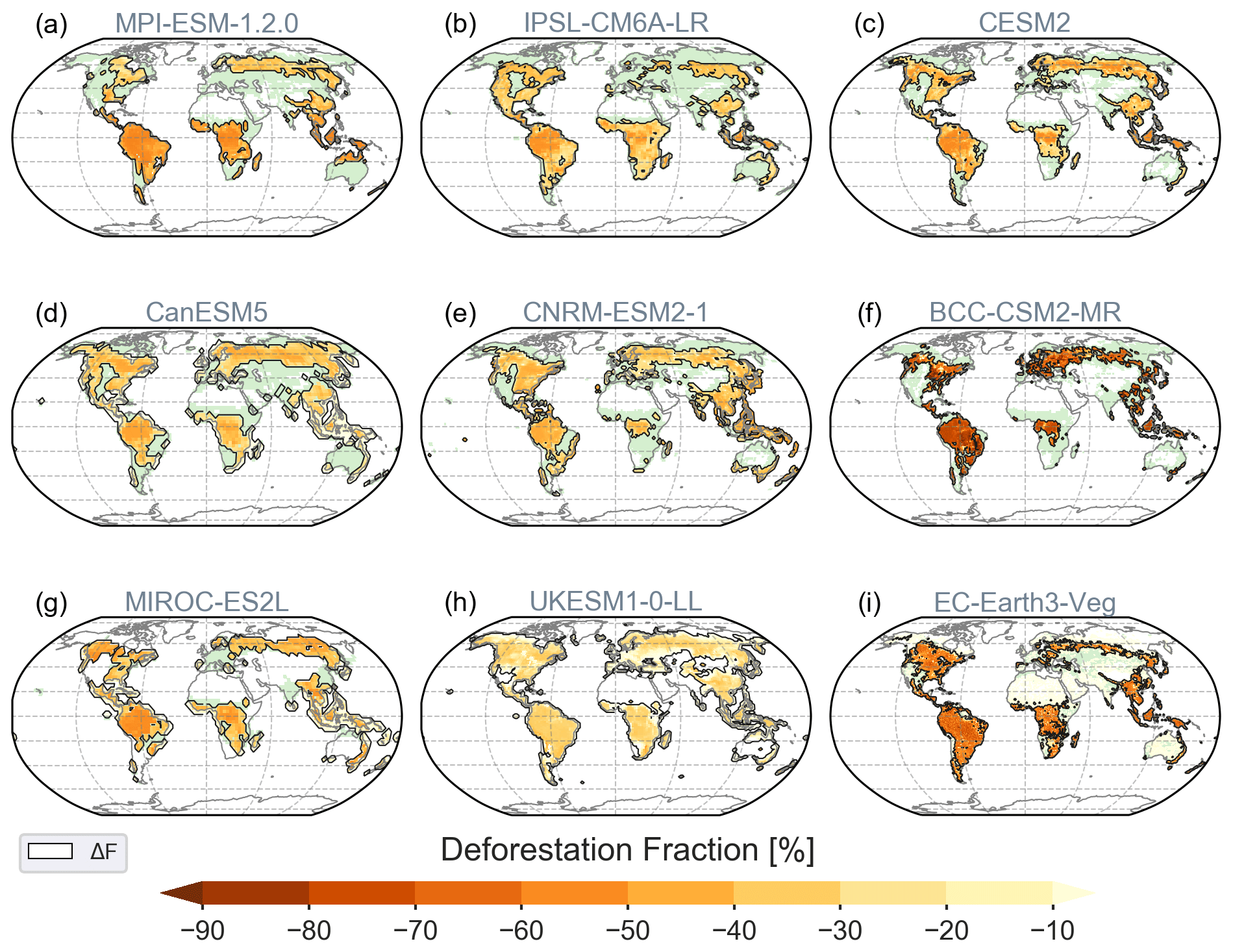
Figure 1Deforestation fractions ΔF in percent (%) of the grid cell area after the forced forest clearing is finished, shown in orange; green colours display the remaining forest extent. A map of the initial forest fractions can be found in the Supplement (Figs. S1 and S2). Contours of the deforestation areas (ΔF) with deforested grid cell fraction exceeding 0.001 % are used in all maps of the analysis.
Deforestation of the top 30 % grid cells with regard to their forested fraction in the piControl simulation of 1850 (see Table 1) leads, as expected, to the largest forest removal in the tropical and boreal zone across all models (Figs. 1 and S2). Regional differences in the spatial pattern of deforestation across models can mainly be attributed to differences in the initial forest cover (36 to 66 Mkm2, Table 1), which is, for instance, almost twice as large in CNRM compared to EC-Earth and BCC. UKESM, CanESM and CESM2 generally remove more than twice as much forest in boreal regions compared to MPI and BCC in North America or IPSL and MIROC in Eurasia. MPI simulates less initial forest cover in temperate regions, in contrast, especially to CanESM, BCC, EC-Earth and CNRM. In EC-Earth, MPI and IPSL, tropical deforestation dominates the global patterns. The spread in initial forest cover highlights the difficulty in implementing any given land use and land cover change scenario (Di Vittorio et al., 2014). Overall, all models successfully perform 20 Mkm2 (range 19.6–21.6 Mkm2) of deforestation after 50 years.
Table 1Changes in the mean state of near-surface temperature (ΔTas), precipitation (ΔPr) and land carbon (ΔcLand) by the end of the deforest-glob simulation globally (both land and oceans) and over areas of deforestation (ΔF) alone. Values in parenthesis denote statistically non-significant values. Values in square brackets for MPI, MIROC and CanESM denote values at the end of simulation (MPI and MIROC at year 150 and CanESM at year 90). Zero-lat denotes the latitude where the change in temperature in response to deforestation turns from temperate/boreal cooling to tropical warming applying an approximated 10∘ running mean. TCRE values (∘C EgC−1) from Arora et al. (2020) applied to global ΔcLand. cLand refers to the sum of cSoil, cVeg and cLitter. Non-significant changes are denoted by “–”.
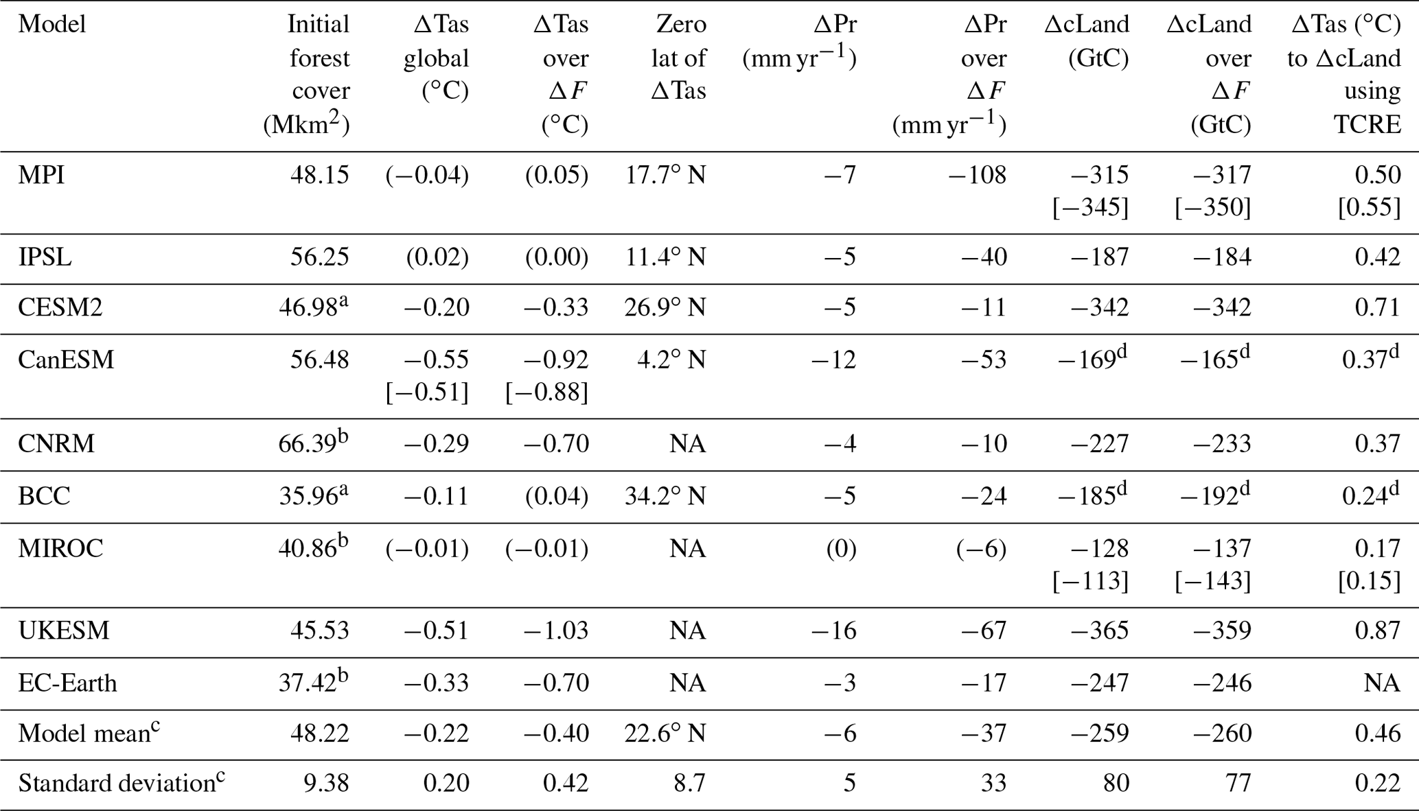
a Based on t0 of the deforest-glob simulation. b Separate file. c Including statistically significant as well as non-significant values. d Only accounting for ΔcVeg in the absence of ΔcLand. NA – not available.
The reconstructed potential forest cover is estimated to be 48.68 Mkm2 in 800 CE or 45.65 Mkm2 in 1700 (Pongratz et al., 2008). The multi-model mean initial forest cover area of 48.22 Mkm2 in Table 1 compares reasonably well with this estimate. The area deforested in the deforest-glob scenario is comparable to the historical deforestation area of 22 Mkm2 between year 800 and 2015, the increase in grazing land from 1850 to 2015 by 20.5 Mkm2, and the projected forest loss of 20.3 Mkm2 between 2015 and 2100 in the land use scenario of SSP5 RCP8.5 (Hurtt et al., 2020). However, in the deforest-glob experiment deforestation occurs over a much shorter period of time, and the geographical locations of deforestation differ.
3.2 Biogeophysical effects
The analysis of biogeophysical effects of deforestation is split into sections on global and regional changes in the mean state by the end of the simulation period and the temporal evolution of the primary energy quantities.
3.2.1 Changes in mean near-surface temperature
Six of the nine models simulate a statistically significant decrease in global near-surface air temperature in response to large-scale deforestation. Results of statistically significant changes (Table 1) range from −0.11 to −0.55 ∘C (multi-model mean −0.33 ∘C) globally as simulated by BCC, UKESM, CanESM, CESM2, CNRM and EC-Earth, while MPI, IPSL and MIROC show no significant changes on the global scale. Over areas of deforestation (ΔTas over ΔF) the cooling is stronger (−0.33 to −1.03 ∘C, multi-model mean −0.40 ± 0.42 ∘C). Globally averaged, BCC simulates the weakest response as a consequence of balancing regional patterns (Fig. 2). Globally and regionally, MIROC shows almost no response of ΔTas to the deforestation forcing since the rapidly regrowing, secondary vegetation is very similar to the original land cover.
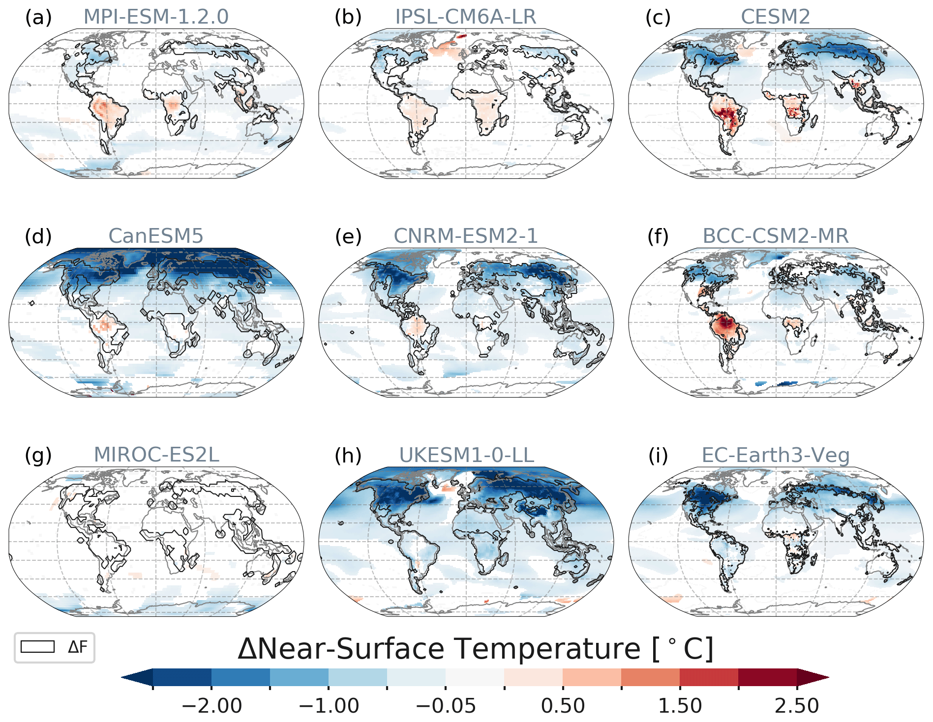
Figure 2Spatial patterns of near-surface air temperature (ΔTas) responses averaged over year 50 to year 79. Only statistically significant changes at the 5 % significance level are shown (modified t test, Zwiers and von Storch, 1995). Contours depict the areas of deforestation (Fig. 1).
The global net decrease in air temperature is dominated by the changes over the oceans and in the Arctic (Fig. 2). Using the surface energy balance (SEB) decomposition approach, we can analyse the contribution of varying energy fluxes to the change in surface temperature (ΔTsurf, Fig. 3f). ΔTsurf is directly related to the balance of surface energy fluxes. However, it might deviate from ΔTas at 2 m height (see also Winckler et al., 2019a) and is therefore shown in Fig. S3 (dashed black lines), which provides a model-wise SEB decomposition. The contributing fluxes are displayed in Fig. S4 (including cloud cover and full and clear-sky longwave radiation).
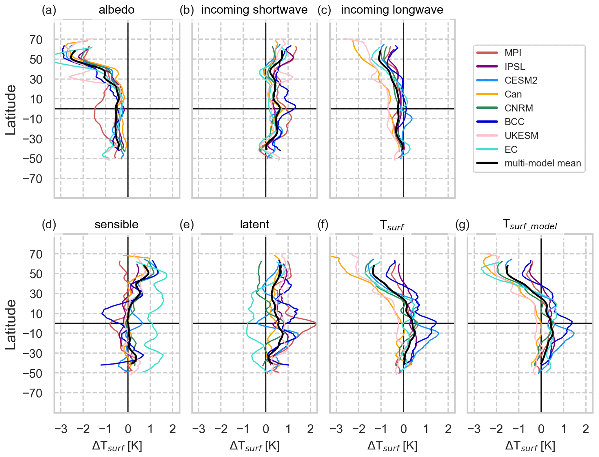
Figure 3Zonally averaged surface energy balance (SEB) decomposition component-wise for every model after deforestation (averaged over year 50 to year 79) including only areas of deforestation (ΔF). Changes in the surface temperature (Tsurf) are expressed as the contribution of changes in available energy (incoming and reflected shortwave and incoming longwave, a to c) and turbulent heat fluxes (latent and sensible, d and e). Tsurf is derived from the SEB decomposition method; Tsurf_model is simulated by each model; The difference of Tsurf_model and Tsurf represents the residual flux accounting for the ground heat flux and subsurface heat storage. An approximated running mean over 10∘ latitude was applied to smooth lines. The multi-model mean is only applied to latitudes at which all models simulate changes. Note that MIROC was not included due to only minor responses to the deforestation signal. A model-wise SEB decomposition including the simulated near-surface temperature (ΔTas) and results from MIROC can be found in Fig. S3.
In the mid- to high northern latitudes all models simulate an increase in albedo in response to deforestation, which induces a cooling (Fig. 3a). This increase in albedo mainly originates from the reduction in snow-masking effect of forests allowing for a denser and longer lasting snow cover towards summer over grasslands that replace forests. Some models even simulate non-local effects: in CESM2, BCC and EC-Earth this effect is carried beyond the geographical regions of deforestation, and in CanESM and UKESM the geographical extent of the cooling is amplified due to a positive sea-ice–albedo feedback over the Arctic Ocean (see Fig. S5). Longwave radiation is reduced across all models northward of 35∘ N mainly as a result of reduced surface temperatures leading to less atmospheric trapping and re-emission of longwave radiation (Zeppetello et al., 2019). This effect dominates over the impact of increasing cloud cover over these latitudes in UKESM, EC-Earth, BCC and CNRM, which contributes with a longwave warming (see Fig. S4 for zonal fluxes, Fig. S6 for total cloud cover and Fig. S7 for downward longwave radiation). UKESM, IPSL and CESM2 produce a “warming blob” in the North Atlantic which in turn enhances sea surface evaporation (Fig. S8) and latent heat fluxes (not shown), possibly due to the increased moisture demand of the atmosphere. This result is in line with the reversed finding by Rahmstorf et al. (2015), who found a “cooling blob” due to the freshwater input from the Greenland ice shield caused by global warming slowing down the meridional overturning circulation.
All models simulate reduction in available energy (due to reduced net shortwave and incoming longwave radiation) over areas of temperate (50 to 23∘ S and 23 to 50∘ N) and boreal (50 to 90∘ N) ΔF (Fig. S4c), which dominate the reduction in temperature response, leading to cooling. The effects of increasing albedo (Figs. 3a and S5) are stronger than the reduction in longwave radiation (Fig. 3c). While net shortwave radiation reduces (Fig. 4c), the incoming shortwave radiation increases north of 40∘ N (Fig. S3b) because the reduced evapotranspiration lowers the atmospheric water vapour content, and this increases the transmissivity of solar radiation through the atmosphere. In the MPI and IPSL models, reductions in cloud cover (Fig. S4f) contribute to enhancement of transmissivity. With less net radiative energy entering the system, less energy is available for the generation of turbulent heat fluxes (latent plus sensible heat, Fig. S4a). At these higher latitudes all models except CNRM simulate decreased latent heat fluxes as not only forests are replaced by less evapotranspirative grassland, but also the atmospheric moisture demand due to the surface cooling and less moisture supply by precipitation reduce this flux. Similarly, most models simulate reduced sensible heat fluxes as a consequence of reduced surface roughness and weaker vertical mixing. Only MPI and MIROC increase the sensible heat flux to balance the greater temperature gradient between the surface and atmosphere following the roughness reduction which is possible as net shortwave radiation is not as much reduced as in other models.
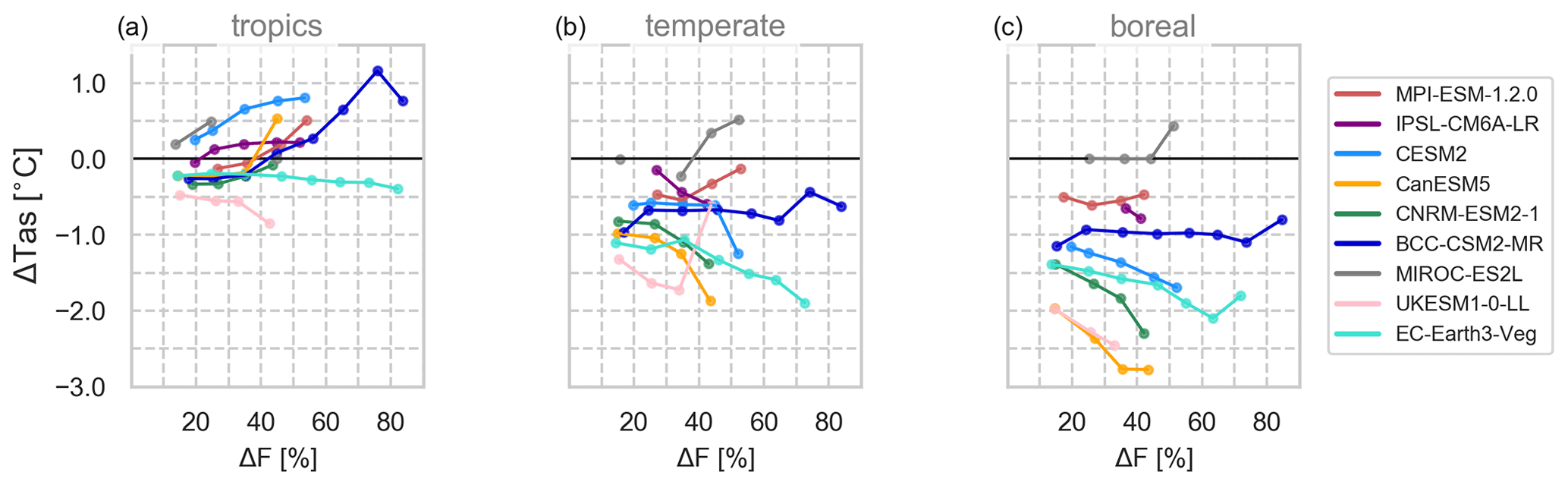
Figure 4Relationship between near-surface temperature changes (ΔTas, averaged over year 50 to year 79) to the final deforestation fraction averaged over all pixels in the (a) tropical (23∘ S to 23∘ N), (b) temperate (50∘ S to 23∘ S and 23 to 50∘ N) and (c) boreal (50 to 90∘ N) region.
The global-scale deforestation-induced cooling is only offset over tropical forests. Here, most models (with the exception of EC-Earth and UKESM) show a warming over ΔF (Fig. 2), since the reduction in evapotranspiration and the decreases in latent heat fluxes dominate the increase in the albedo due to replacement of forests by grasslands (Figs. 3a and S5). However, the geographical patterns differ across models. All models simulate an increase in albedo in the tropics as brighter grasses replaced the darker forests. However, more incoming shortwave radiation (Fig. S3b) due to reduced cloud cover (Figs. S4f and S6) more than compensates for the reduction in incoming shortwave radiation associated with an increase in albedo (Fig. S3a) in IPSL, CanESM, CNRM and BCC. UKESM is the only model that simulates tropical cooling at the surface and at 2 m height, with reduction in incoming shortwave radiation due to increasing albedo more than compensating for the reduction in latent heat and roughness decreases leading to overall cooling. This dominant effect of albedo changes is also observed in HadGEM2-ES, which shares similar model components (Robertson, 2019).
In CESM2, in the equatorial tropics, evaporation increases (Fig. S8). This unintuitive response may be due to the fact that C4 grasses, which were parameterized for dry regions, are overproductive when they replace forests in the moist deep tropics. This cooling effect is balanced by reduced sensible heat fluxes and increased net shortwave radiation due to less cloud cover resulting in a net warming (Figs. 2c and 3c). Similarly, in EC-Earth evaporative cooling (Figs. 3e and S8i) prevails from 30∘ N to 50∘ S since unmanaged grasses show strong increases in leaf area that in turn increase the transfer of soil moisture to the atmosphere. However, this cooling is overcompensated for by the strongest decrease across models and latitudes in sensible heat fluxes (Figs. 3d and S4e) as a consequence of a very low surface roughness of grasses. BCC simulates the strongest temperature increases over the tropical region across all models (Figs. 2f and S3f), leading to a net increase in temperature averaged across all areas of ΔF. In the Amazon region this is mainly caused by an initial surface drying due to reduced evapotranspiration and increased sensible heat flux. This strengthens the circulation over the northern Amazon, supporting increased vertical convection of hot air that in turn causes horizontal advection of moist air from the tropical Atlantic (note that evaporation from the land decreases over the northern Amazon, Fig. S8f) – this behaviour is similar to deforestation responses found in CESM1 (Chen et al., 2019). This leads to increased cloud formation, which increases incoming longwave radiation (with all-sky surface longwave radiation being larger than clear-sky surface longwave radiation, Fig. S7f).
Comparing ΔTas and ΔTsurf (Fig. S3) reveals that there can be large differences among both variables. In CNRM, the surface warming of ΔTsurf, which is dominated by reduced evapotranspiration, is not seen in ΔTas at 2 m height (Fig. S3e). In EC-Earth the effect of reduced sensible heat fluxes causes warming at the surface (Fig. 3i) which is not mixed upwards to the 2 m level (Fig. 2i) where a cooling is observed. MPI and CanESM show the smallest deviations in ΔTas and ΔTsurf.
The SEB approach applied here neglects the ground heat flux on longer averaging periods, subsurface heat storage or changing emissivity. However, inferring the difference between modelled and analytically determined Tsurf we see remaining negative differences in energy fluxes at higher latitudes in IPSL, CNRM and EC-Earth (difference of Tsurf_model and Tsurf, Fig. S3). This deviation from the simplifying assumption of our SEB approach assuming zero changes in the above-mentioned properties and fluxes needs further investigation, which is beyond the scope of this paper. Although the impact of the simulation height of Tsurf_model and calculation height of Tas is done differently across the models (see Sect. 2.3), we cannot coherently attribute the observed gaps between ΔTsurf_model and ΔTsurf or ΔTas and ΔTsurf to this. For example, EC-Earth and CanESM defined Tsurf_model to be at the surface and Tas to be 2 m above the surface, but while EC-Earth simulates clear deviations between these variables and also Tsurf, differences are almost negligible in CanESM (Fig. S3).
In four out of nine models that simulate tropical warming and temperate/boreal cooling in response to deforestation the switch in sign of ΔTas from warming to cooling ranges from 11.4∘ N in IPSL to 34.2∘ N in BCC (multi-model mean 22.6∘ N) if changes in ΔTas over ΔF (Fig. S3, black dashed lines) are zonally averaged (Table 1). This change in sign of the temperature response due to the biogeophysical effect is an important metric which indicates that the biogeophysical effects of re/afforestation would result in cooling south of this latitude, in addition to a global cooling effect due CO2 removal from the atmosphere. Because the other five models show the cooling effect of deforestation at all latitudes due to non-local effects, this estimate is highly uncertain with a standard deviation of at least 10∘ (Table 1).
Overall, the local response over deforested areas is a reduction of available energy (net shortwave plus downwelling longwave radiation, Fig. S4b) across all models at higher latitudes (by −5 to −20 and −0.5 W m−2 in MIROC) due to snow-related albedo feedbacks of brighter grasses versus darker trees. At lower latitudes, the models' response is more diverse mainly due to differences in cloud formation (−5 to +10 W m−2, Fig. S4f). As a result of less energy being available, turbulent heat fluxes reduce across all models and latitudes (by −1 to −12 W m−2, Fig. S4a). Most models simulate decreased latent heat fluxes over less evapotranspirative grasses (Figs. S4d and S8). Only two exceptions were found where grass parameterizations lead to higher latent heat fluxes (CESM2 and EC-Earth). Most models simulate a reduction in sensible heat fluxes over temperate and boreal grasslands which replace forests as roughness over grasses is lower, which weakens vertical mixing. These findings are in line with those of Winckler et al. (2019b), who find a dominating role of surface roughness for local effects of deforestation. MPI and MIROC simulate an increase in sensible heat as net radiation reductions in these models are small and energy is partitioned preferentially towards the sensible heat flux. In the tropical region, stronger sensible heat fluxes are seen everywhere in response to deforestation, where ΔTsurf increases due to a stronger temperature gradient between the surface and the atmosphere. In CanESM, EC-Earth, and locally in CESM2 and BCC, however, the effect of a strongly reduced roughness outweighs the impact of the temperature gradient.
Previous studies on the temperature effects of large-scale or historical deforestation have shown that the locally induced changes in albedo after boreal deforestation are almost balanced by concurrent changing turbulent heat fluxes. However, the increased boreal albedo can also induce a non-local cooling over land and oceans via advection of cooler and dryer air (Chen and Dirmeyer, 2020; Davin and de Noblet-Ducoudré, 2010; Winckler et al., 2019a). Like in other multi-model studies on the biogeophysical effects of deforestation, it is difficult to separate local and non-local effects without further separation experiments. However, we also find a mean cooling across all models globally and locally over the areas of deforestation. Only MPI, IPSL and BCC simulate weaker non-local cooling effects, thus almost balancing global mean temperature effects of tropical warming and boreal cooling.
Still a key question is how models simulate the impact of deforestation on the turbulent heat fluxes (de Noblet-Ducoudré et al., 2012; Pitman et al., 2009), depending not only on the plant-physiological behaviour (e.g. stomatal conductance, growing seasons, leaf area index) but also on parameterizations of surface roughness and the soil hydrology schemes.
3.2.2 Forest sensitivity (FS) of ΔTas
The sensitivity of the models to the imposed deforestation signal by the end of the simulation period can be quantified in terms of the temperature change (ΔTas) per unit fraction of grid cell deforested (Fig. S9) or per unit area of deforestation (Fig. S10). We therefore call it the “forest sensitivity” (FS) to ΔF.
In the temperate and boreal regions, UKESM, CanESM and EC-Earth show temperature changes of more than −20 ∘C frac−1; CESM2, CNRM and BCC of −10 ∘C frac−1; and MPI and IPSL of up to −4 ∘C frac−1 (Note that the colour bar range is limited and extreme values are not shown). Per 103 km2 of deforestation within one grid cell, UKESM and EC-Earth simulate temperature changes of more than −2.5 ∘C; CESM2, CNRM and BCC of more than −1.3 ∘C; and CanESM, MPI and IPSL of less than −0.6 ∘C 103 km−2. In the tropics, BCC and CESM2 show temperature increases of over 4 ∘C frac−1, MPI and IPSL show temperature increases of less than 2 ∘C frac−1, and EC-Earth and UKESM show decreases of up to −2 ∘ frac−1. Per change in 103 km−2 forest area, only BCC and EC-Earth show detectable changes of more than 0.5 ∘C.
However, FS not only reflects local but also the superimposed non-local effects caused by feedback mechanisms. In the tropical region where non-local effects are smaller, we still see some differences in intensity. In particular, CESM2 and BCC and to a smaller degree MPI reveal areas of stronger sensitivity to deforestation in the tropics than elsewhere (up to 8, 6 and 4 ∘C frac−1, respectively). IPSL, CanESM and CNRM show smaller sensitivities and patterns of coupling also due to the superimposed non-local effects in the latter two models.
To draw more broad conclusions, FS is averaged for every 10 % increase in ΔF per climate zone (Fig. 4). Over tropical regions (23∘ S to 23∘ N, Fig. S11), MPI, CanESM, CNRM and BCC reveal increasing warming to increasing ΔF, which weakens and even stagnates in CESM2 and IPSL, respectively. On average these models show a tropical warming response of 0.27 ∘C frac−1(derived from Fig. 4a). UKESM and EC-Earth simulate increasing cooling with a larger deforestation extent of −0.34 ∘C frac−1. At higher latitudes (>50∘ N, Fig. 4c), five models show an increasing cooling with increasing ΔF (mean −1.31 ∘C frac−1), which is increased by polar amplification. However, MPI, MIROC, BCC and EC-Earth show reverse tendencies at higher ΔF. Over temperate regions (Fig. 4b), there is a more widespread cooling (mean −0.78 ∘C frac−1) due to mingling effects of different biomes, climate zones and generally smaller forest areas.
Previous studies have argued that the local temperature response to complete deforestation is stronger the smaller the initial forest cover was, and thus non-linear (Li et al., 2016; Pitman and Lorenz, 2016; Winckler et al., 2017).
Only CESM2 and IPSL seem to produce the suggested non-linear, saturating behaviour over tropical regions where non-local effects are smaller (see Fig. 2), and a clear linear behaviour cannot be found with any of the models.
However, drawing conclusions on the (non-) linearity is difficult. In our setup, ΔF reflects the top 30 % of forested grid cells and thus links to the initial forest cover but without capturing the potential effects of completely cleared grid cells, smaller forest fractions, distinct ecozones or isolation from non-local feedback effects.
At a higher level of spatial precision including climate and ecozones, results like the ones presented here could be used to generate lookup tables for climate responses of each model to a given level of deforestation. These would provide computationally inexpensive tools to draw fast conclusions on the climate effects of deforestation in, for example, future land use scenarios. However, in some models the responses show a non-linear behaviour not only to local coupling mechanisms but also due to climate feedbacks acting at the global scale. This superimposed, non-local signal should be isolated for models with strong Arctic amplifications (here CanESM, CNRM, UKESM, CESM2 and EC-Earth) to derive local climate responses. In addition, it would be preferable to use results from longer simulation periods once the models have equilibrated for such lookup tables.
3.2.3 Temporal analysis of ΔTas
The results presented so far do not take into account whether the models have reached equilibrium by the end of the simulation period. Globally, UKESM, CNRM, CanESM and EC-Earth simulate a linear response to the deforestation signal with CanESM, EC-Earth and CNRM showing a continuing downward trend after the end of deforestation, while UKESM stabilizes over ΔF and globally (Fig. 5a). BCC simulates a more or less constant temperature increase over ΔF dominated by tropical warming, though the global signal is a slight cooling. MIROC drives hardly any change in ΔTas for any level of deforestation. MPI, IPSL and CESM2 show only small responses on the global scale due to balancing signals, but regionally ΔTas scales with the intensity of deforestation. Over South America, BCC, CESM2, MPI and IPSL simulate a linear increase while UKESM, CNRM and EC-Earth simulate decreases in Δtas with ΔF (not shown). In the boreal region, all models but MIROC simulate a linear decrease with ΔF over time, which clearly continues after 50 years in CanESM, EC-Earth and CNRM over North America and CanESM over Eurasia.
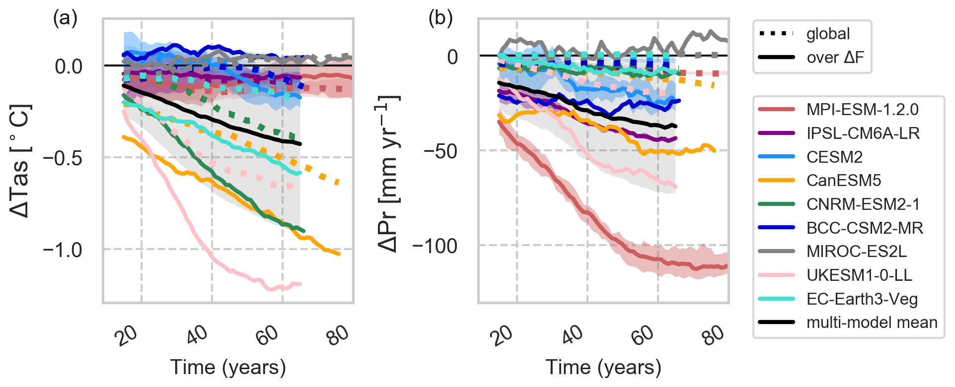
Figure 5Time series of temperature (a) and precipitation changes (b). Solid lines depict changes over areas ΔF, while dotted lines depict global changes. A 30-year moving average is applied. The black line shows the multi-model mean with 1 standard deviation in shaded grey.
The temporal evolution of ΔTas reveals not only the sensitivity of models to large-scale deforestation but also the strength of non-local high-latitude feedbacks. For most models it would have been beneficial to extend the simulation period to allow the climate variables to reach equilibrium. The two models providing 150 years of data, MPI and MIROC, are less sensitive models without strong feedbacks and thus equilibrate quickly. For UKESM, recovering forests in the remaining parts of the deforested grid cells shape the evolution of the signal.
For models that provided several ensemble members of the deforestation experiment (MPI, IPSL and CESM2) we calculated the time of emergence (ToE). In the tropics, near-surface temperature changes emerge over the regions of strongest deforestation before the end of the first 50 years of the simulation (Fig. 6). Interestingly, the signal propagates from the centre of deforestation to the edges in the tropical zone. In the central tropics, the signal becomes robust (that is, exceeds the signal-to-noise ratio (SNR) of 2) with up to 20 % to 35 % of deforestation still left (Fig. S12). This hints at the advection of temperature changes towards the centre of deforested area due to non-local effects. In boreal zones, CESM2, and to a lesser degree in MPI, demonstrates signals propagating westwards starting from the boreal east coasts with about 30 % and 10 % of deforestation, respectively, still left (Fig. S12). The main attributors here are the westerly winds that carry the modified air by deforestation from the west to the east coast of the continent where the signal is therefore strongest and emerges earlier. In CESM2, Arctic amplification further amplifies this process (see Sect. 3.2.1), leading also to responses outside ΔF. In MPI and IPSL, the advection of temperature changes from neighbouring grid cells is limited to areas of ΔF. In the majority of areas, the signal takes more than 50 years to emerge despite the strong imposed deforestation forcing (Fig. 6 green and blue colours).
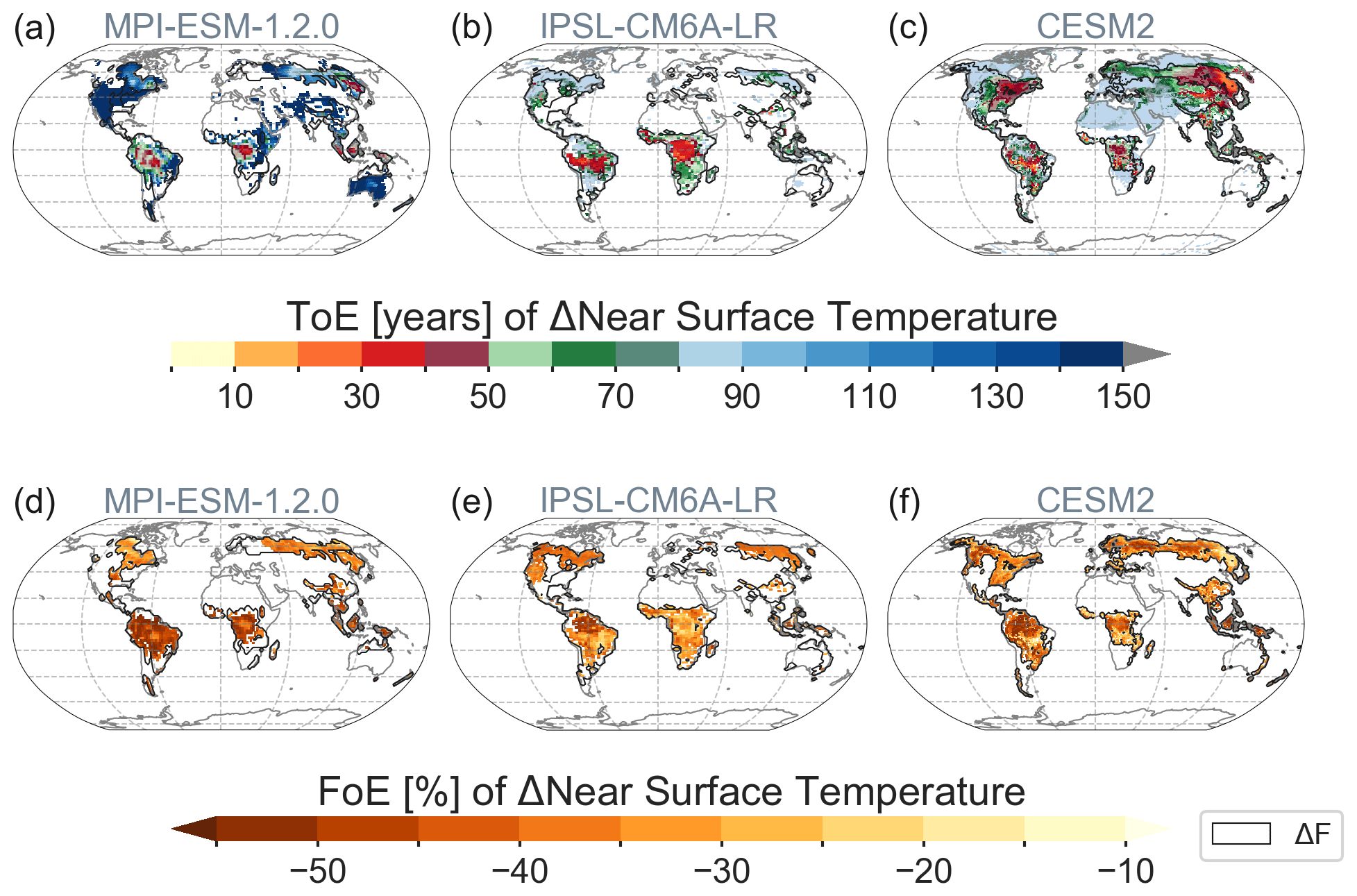
Figure 6(a–c) Time of emergence (ToE) of ΔTas and (d–f) equivalent fraction of emergence (FoE) of ΔTas. Only statistically significant areas as found in Fig. 2 are shown; oceans are masked out.
The results of the ToE analysis have to be treated with caution since only a few ensemble members were available, and thus uncertainty remains high. However, following up on the earlier analysis (Sect. 3.2.1), the observed patterns make sense from a causal perspective. After 30 years, all three models demonstrate a propagation of signals from the centre to the edges of ΔF, and two show a westward propagation across the boreal zone. This emphasizes the importance of non-local biogeophysical effects during and after large-scale deforestation (Chen and Dirmeyer, 2020; Pitman and Lorenz, 2016; Winckler et al., 2019b). FoE is more universally applicable across models as the same amount of deforestation can happen at a different time in each model. Notably, while ToE patterns of ΔTas are very diverse across models, the FoE patterns are more alike, especially in the tropics. These results lead to the conclusion that even after large-scale deforestation of one-third to half of the grid cell's forests, the signal only becomes robustly detectable after a few decades as climate variability and mediating effects from the ocean have to be overcome (Davin and de Noblet-Ducoudré, 2010). The applied method based on ensemble trends gives an optimistic estimate of ToE compared to alternative approaches based on multi-ensemble or temporal means relative to the variability of a reference period (Fig. S13, note that SNR was lowered to 1).
Our results have important implications for ongoing land cover changes and climate policies. Between 2001 to 2018, 3.61 Mkm2 of forests was cleared (Hansen et al., 2013; and http://earthenginepartners.appspot.com/science-2013-global-forest, last access: 18 May 2020); thus the deforestation rate was about 20 % of that applied in this study. Our results suggest that the detection of climate effects of this recent deforestation would possibly take decades. Likewise, climate response times to the reversal of deforestation as a mitigation measure would be long compared to climate policy timescales.
3.2.4 Changes in precipitation
The global net effect of precipitation changes over ΔF is negative across all models ranging from −10 to −108 mm yr−1 (mean −37 ± 33 mm yr−1, Table 1). All models show shifts of atmospheric patterns over the oceans and distinct changes over ΔF (Fig. 7). Again, MIROC is the least sensitive model with only minor increases over South Africa and Alaska.
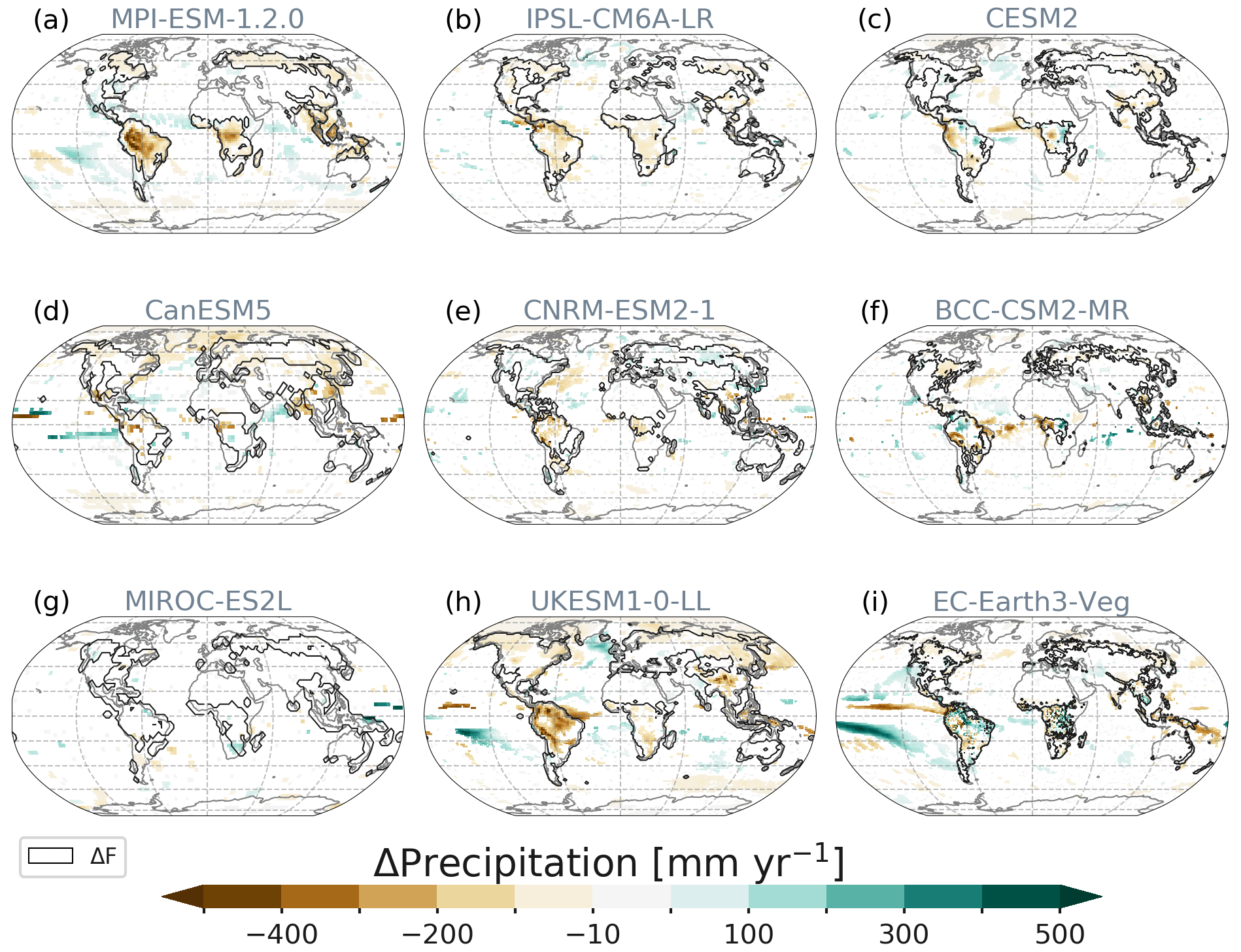
Figure 7Spatial patterns of precipitation responses averaged over year 50 to year 79. Only statistically significant changes shown. Contours depict the areas of deforestation (Fig. 1).
Over time, MPI, UKESM and IPSL simulate linear responses to the deforestation signal with only MPI showing global stabilization after ending forest removal (Fig. 5b). Other models exhibit longer time periods (CanESM and MIROC) of continuing positive or negative changes depending on the region. For example, over North America (not shown), CanESM simulates a downward and MIROC an upward trend in precipitation.
The strongest global mean reduction of moisture transfer to the atmosphere via evapotranspiration (Fig. S8) and resulting precipitation over ΔF is found in MPI, followed by UKESM, CanESM and IPSL. Generally, these decreases result from the replacement of forest by less evapotranspirative grasses. Precipitation increases occur mostly outside deforested regions but also on small scales over areas of ΔF in CESM2, CNRM, BCC and EC-Earth for different reasons: in CESM2, C4 grasses replace forest in tropical regions which are parameterized to be productive under unfavourable climate conditions (e.g. too try or hot) and, hence, are overly productive in tropical zones, leading to transpiration increases. EC-Earth simulates increases in the tropics following increased evapotranspiration (ET) due to a strong increase in leaf area. CNRM is the only model simulating precipitation increases over ΔF at northern latitudes providing moisture for enhanced evapotranspiration during snow-free months. In BCC, local vertical convection in the Amazon region causes horizontal advection of moist air from the Atlantic and west Amazon, which locally increases precipitation there (see Sect. 3.2.1).
Over tropical ΔF, most models show a linear relationship with relative temperature increases correlating with relative precipitation decreases and vice versa (Fig. S14). UKESM shows a linear decrease in ΔPr with a decrease in ΔTas. Due to the above-mentioned model specifications, CESM2 and BCC show a very weak relationship between ΔTas and ΔPr over tropical ΔF, with also positive ΔPr paired with positive ΔTas. Over boreal ΔF, most models simulate decreases in ΔPr correlated with decreases in ΔTas, while in CNRM ΔPr increases despite the cooling air.
Global deforestation affects precipitation by altering circulation patterns and by changing the moisture inputs from the surface to the atmosphere. The SEB analysis (Sect. 3.2.1) demonstrated how new plant types govern the land–atmosphere interaction via turbulent heat fluxes. In most cases we could infer a causal link between changes in turbulent heat fluxes, longwave radiation linked to cloud cover and precipitation, which is in line with previous studies (e.g. Akkermans et al., 2014; Lejeune et al., 2015; Spracklen et al., 2012). While most models simulate moisture decreases as less productive and evapotranspirative grasses replace trees, some models simulate local increases due to advected moisture (e.g. BCC) or favourable parameterizations of grasses (e.g. CESM2 and EC-Earth).
3.3 Biogeochemical changes
3.3.1 Changes in mean and temporal development of carbon pools and fluxes
Land carbon (cLand, the sum of vegetation, soil and litter carbon) losses range from −169 to −338 GtC until the end of the deforest-glob simulation. Note that CanESM and BCC were excluded in this calculation due to a major divergence from the protocol. By the end of the experimental period the spread across models increases to −144 to −350 GtC, with UKESM and MPI simulating continuing declines and MIROC simulating increases. The multi-model mean decreases from −191 GtC after 50 years (mean over year 45 to 54) to −203 GtC after 75 years (mean over year 70 to 79, Table 1) after the start of the simulation. If only models were included that followed the protocol closely (MPI, CNRM and CESM2), the multi-model mean would be −282 GtC after 50 years and −300 GtC after 75 years. The spatial patterns of ΔcLand are displayed in Fig. S15. The spread across models is the result of several factors that make the model behave differently.
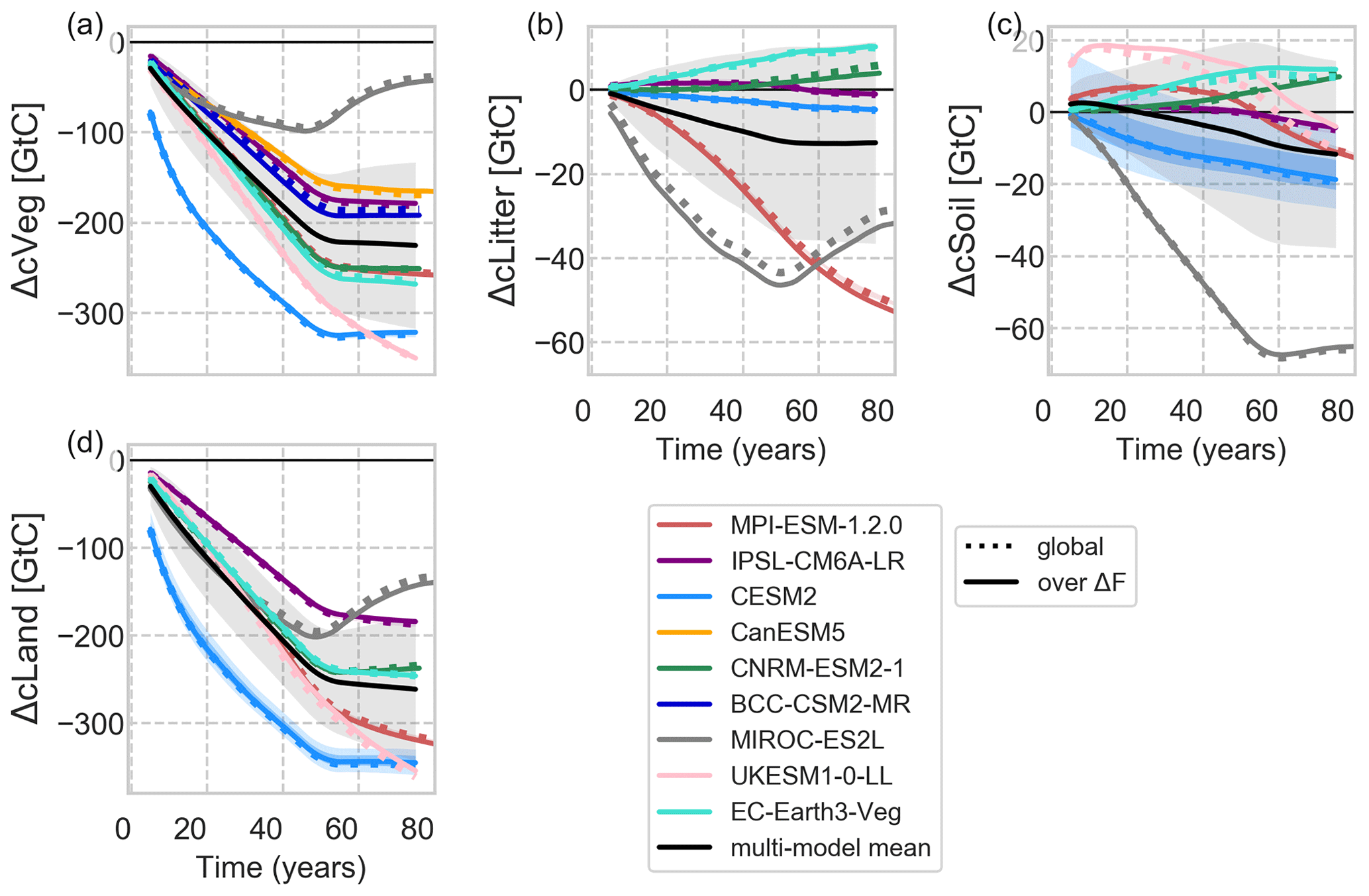
Figure 8Changes in carbon cycle pools over time smoothed by a 10-year moving average. Note that for CanESM and BCC only ΔcVeg could be analysed. ΔcLand refers to the sum of ΔcSoil, ΔcVeg and ΔcLitter. The black line shows the multi-model mean with 1 standard deviation in shaded grey.
For all models but MIROC, it is mainly the changes in vegetation carbon (ΔcVeg) dynamics that dominate changes in cLand followed by changes in litter carbon (ΔcLitter) and soil carbon (ΔcSoil, Fig. 8).
In UKESM dynamic vegetation adjustments in the remaining natural parts of the deforested grid cells drive the continuing decline and weak recovery of ΔcVeg as a consequence of strong cooling followed by stabilizing climate, respectively (Fig. 8a and b). Below-ground carbon is transferred to the fast soil carbon pool (ΔcSoilFast, residence time of a year), which reduces with ongoing deforestation (Fig. S17c). Fast soil carbon decays and thereafter accumulates in the medium soil carbon pool (ΔcSoilMedium, residence time of several decades; Fig. 17b). The development of cLitter and heterotrophic respiration (rh) reductions and the subsequent development of all soil carbon pools correlate with the progression of deforestation and vegetation recovery afterwards. Note that for UKESM below-ground carbon from coarse roots is removed from the system and not transferred to the soil carbon.
In MIROC, because the vegetation type was fixed as woody types in the deforestation, forest recovery started soon after the deforestation process. As a result, the magnitude of ΔGPP is moderately decreasing among the models (Fig. 10a) and ΔcVeg recovers as secondary woody vegetation, leading to the positive large net ecosystem productivity (NEP; Fig. 10d).
CESM2 shows a steep decline in cLand, which is mainly caused by the initial vegetation loss and enhanced fire activity (carbon emissions by fire, ΔfFire) during deforestation of tropical forests due to degradation fires from deforestation (Li and Lawrence, 2017). The sudden initiation of deforestation fires in the Tropics contributes to emissions of 12 GtC yr−1 at the beginning of the deforestation period and levelling off at around 1.7 GtC yr−1 after 50 years (Fig. 10e), with the highest values in the tropics (Fig. S16). These initial deforestation fires cause GPP to drop for the first two decades before the overly productive C4 grasses in CLM5 (Lawrence et al., 2019), especially in the deep tropics (Fig. 9), start to compensate for the carbon losses. ΔcLand saturates around −342 GtC, with a minor negative drift after deforestation stops. The path is slightly non-linear as the tropical grasses lead to recovery in ΔcLand after deforestation stops. In combination with a constant decline of heterotrophic respiration (Fig. 10c), net ecosystem productivity (ΔNEP, Fig. 10d) turns slightly positive by the end of the simulation period.
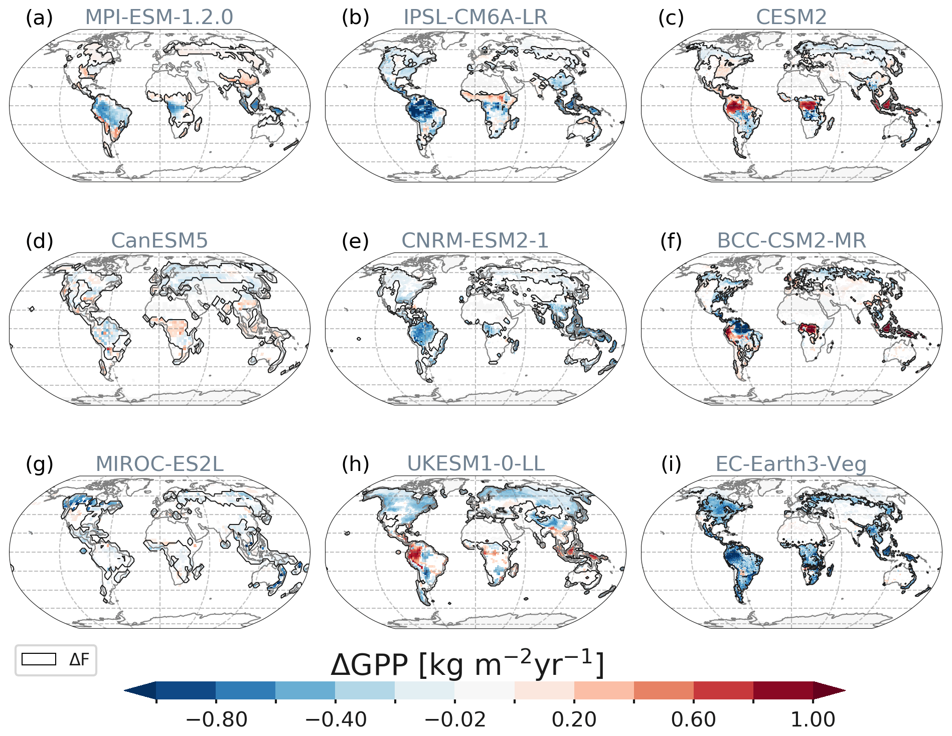
Figure 9Spatial patterns of ΔGPP responses averaged over year 70 to year 79. Only statistically significant changes at the 5 % significance level are shown. Contours depict the areas of deforestation (Fig. 1).
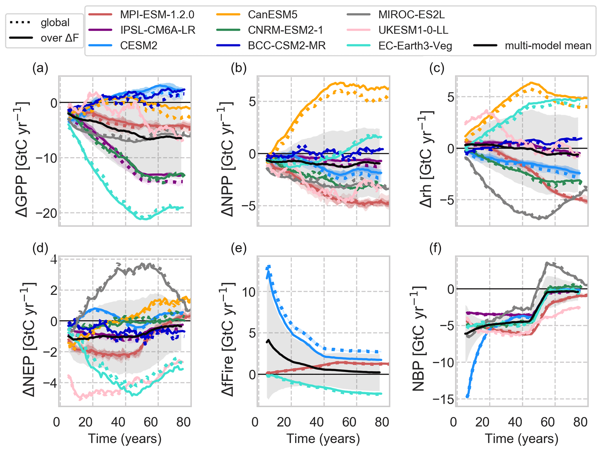
Figure 10Changes in carbon fluxes over time smoothed by a 10-year moving average. GPP and NPP are the gross and net primary productivity, respectively; rh is the heterotrophic respiration; NEP is the net ecosystem productivity; fFire denotes the emissions by fire; and NBP denotes the net biome productivity. NBP is based on year-to-year variations in ΔcLand and thus not provided for CanESM and BCC. The black line shows the multi-model mean with 1 standard deviation in shaded grey.
The slight continuing downward trend of ΔcLand in MPI is dominated by changes in the tropics (not shown). As grasses replace trees, ΔNPP is reduced strongly (Fig. 10b), and consequently litter pools are reduced as well (in fact, MPI has the strongest NPP reduction across models with up to −2.2 GtC yr−1 found in the tropics). Grass litter flux is not only smaller in amount, but also of changed quality, leading to faster decomposition. Like in UKESM, the gain of fast soil carbon pool due to root decomposition during the first 50 years has only a minor effect in the long term (Fig. S17). Fire activity is fostered globally as grasses are more fire-prone than trees. In MPI, fire activity is enhanced because of a warmer tropical and globally drier climate (Fig. 10e), slowly diminishing land carbon pools at a similar rate as in CESM2 (∼1.3 GtC yr−1). Regional precipitation reductions cause heterotrophic respiration to decrease even more strongly than ΔNPP, resulting in positive ΔNEP by the end of the simulation period.
EC-Earth and CNRM seem to behave similarly in terms of ΔcVeg, ΔcLitter and ΔcSoil at the global scale. However, regionally the models show fundamentally different responses. EC-Earth simulates higher deforestation rates in the tropics with subsequent higher cVeg loss than in CNRM and vice versa for higher latitudes. Interestingly, ΔcLitter and ΔcSoil increase in EC-Earth globally and CNRM in higher latitudes. In CNRM, grasses produce more below-ground litter fall than trees (due to a higher root-to-shoot ratio), which accumulate, accompanied by lower overall Δrh fluxes, in all soil carbon pools.
In EC-Earth, increases in cLitter and cSoil are partly caused by the deforestation itself since portions of root and, against protocol, leaves and wood biomass are left on-site for decay. In addition, reductions in autotrophic respiration of grasses more than compensate for GPP losses due to deforestation, leading to a positive ΔNPP and thus more litter. This litter is further contained as fire emissions in this model are reduced compared to the previous forest landscape ( GtC yr−1 globally). Even the substantial heterotrophic respiration increases due to local moisture input combined with mild cooling can therefore not deplete cSoil.
IPSL shows the smallest response in land carbon, which is dominated by cVeg changes and hardly by any changes in soil or litter carbon pools (Fig. 8). The exception is in central Africa, where the higher NPP of grasses increases the litter flux affecting mainly the long-term soil carbon pool (not shown).
In BCC, tropical changes dominate the global average with the highest observed ΔGPP across models, which is, however, diminished by a similarly high soil respiration flux, resulting in a negative global ΔNEP throughout the simulation period (Fig. 10d). Only in the northern Amazon region, GPP is reduced under high temperatures and despite the observed precipitation increase (Fig. 7). BCC is the only model that simulates cVeg increases outside ΔF in the temperate regions where cooling and precipitation increases overlap, leading to a higher ΔGPP.
From CanESM, we only investigate ΔcVeg and carbon fluxes since carbon was not transferred to the atmosphere as requested by the protocol but to a great proportion left on-site for decay. Still, CanESM shows a very interesting behaviour that diverges from the other models: CanESM simulates a uniform global increase in NPP (Fig. 10b) associated with the highly productive C4 grasses, especially in the tropics (Fig. 9d). The increase in NPP is accompanied by almost as strong heterotrophic respiration increases (as a consequence of increased litter and soil carbon pools), resulting in net ecosystem carbon gains. GPP changes are, however, not obviously different with mainly less productive grasses everywhere but in Africa and south-east Asia (Fig. 9d), meaning that autotrophic respiration of grasses decreases more than in all other models after deforestation.
The net biome productivity (ΔNBP = ΔtcLand with Δt referring to the year-to-year changes in cLand, Fig. 10f) summarizes the effect of land carbon fluxes. In that, all models show similar carbon fluxes of −4.45 ± 1.07 GtC yr−1 during deforestation except for CESM2, with dominating influences from ΔfFire. After the end of deforestation, the ΔNBP reduction declines on average to −0.45 ± 1.06 GtC yr−1. The outliers MPI (continuous reductions of rh) and UKESM (recovering ΔNPP) show a positive trend, thus initiating a slowdown of the loss in ΔcLand opposed to MIROC in which Δrh increases with the growth of secondary vegetation.
Land carbon changes emerge as a signal within the first 10 years in most places (Fig. S18). MPI and IPSL show more distinct patterns at the outermost edges of deforestation, where 30 years pass before ToE occurs. In IPSL and CESM2, many patches outside ΔF show ToE of up to 50 years; however, changes are smaller than ± 0.5 kg m−2 in these areas. ToE of ΔGPP (Fig. S19) is more interesting. ΔGPP is uniformly affected by the replacement of trees by grasses but influenced also by the changes in local climate. In MPI and IPSL, the earliest ToE values appear where strong GPP reductions are observed (Fig. 9), while in CESM2 these locations experience strong GPP increases in this time (10–40 years). Changes in climate impose their signal, and thus similar patterns of propagation can be observed as for ToE of ΔTas.
Although forest removal was implemented in a similar way across models, the trajectory and spatial patterns of carbon changes differ strongly. The major part of the land carbon model spread stems from the removal of vegetation carbon based on the differences in initial forest distribution and carbon densities. A similar divergence across multiple models but of lower magnitude was already found for a previous study investigating the effect of future land use and land cover changes on the carbon cycle in CMIP5 models (Brovkin et al., 2013). The changes in ΔcLand (−260 ± 74 GtC) in the deforest-glob simulation are ∼25 % higher than the estimated historical emissions of 205 ± 60 GtC from land use and land cover changes and wood harvest and wood products between 1850 and 2018 (Friedlingstein et al., 2019).
The loss of land carbon follows a similar trajectory at the global scale, with only vegetation recovery (MIROC, UKESM) and grass parameterization (CESM2) causing non-linearities. We find that not only whether fire is represented (MPI, CESM2, EC-Earth) or not can have substantial effects on the NBP and thus overall carbon losses but especially how it is implemented. In CESM2 fire is used as a deforestation tool, while it only depends on litter fluxes in MPI and EC-Earth. In the latter model, fire activity decreases with the expansion of grassland opposed to the other two models. To narrow down the sign and magnitude of fire emissions thus needs further consolidation by incorporating observational data. The protocol allowed models to simulate dynamic vegetation processes outside the deforestation area based on the assumption that the time horizon of the experiment was too short for climate change effects to affect the remaining woody vegetation (Lawrence et al., 2016). UKESM disproves this assumption since forest cover continuously declined in the remaining part of the grid cell. The separation of land carbon pools by land cover type would have therefore been advantageous. Across all models that witness a declining or constant fast soil carbon pool with the onset of deforestation (CESM2, IPSL, MIROC), the fate of below-ground plant materials (roots) remains unclear considering that root biomass is about one-fifth of the above-ground biomass (Lewis et al., 2019).
The analysis of CMIP5 models revealed that substantial uncertainty in model responses was due to implementation differences (i.e. land use patterns, Boysen et al., 2014; Brovkin et al., 2013). Having a very simple experimental protocol of replacing trees with grasses, we now show that the underlying processes themselves also explain large parts of the model spread. Strong or weak model responses may originate from including or not representing certain processes explicitly, e.g. fire activity or soil biochemistry. Our analyses also highlighted the relevance of the comparative response of different vegetation types. While most evaluation is done for total land carbon stocks and fluxes, assessment of land use change requires adequate representation of individual land use/cover types at each location relative to each other. This highlights the need for improving the process understanding of soil carbon dynamics (e.g. Chen et al., 2015; Don et al., 2011; Giardina et al., 2014; Luo et al., 2017), fluxes (Atkin et al., 2015; Huntingford et al., 2017) and biomass carbon stocks (Erb et al., 2017) using observations and field experiments.
3.3.2 Forest sensitivity (FS) of land carbon
Similarly to ΔTas, the FS of ΔcLand is analysed. Across models, MIROC is the most sensitive with local land carbon losses per fraction of deforestation (Fig. S20; note that the extreme values are not shown in the colour bar) of ∼ −95 GtC in boreal North America, followed by UKESM with GtC and other models with −40 to −50 GtC. On average, UKESM, CESM2 and MPI amount to −16 GtC while the other models stay around −9 GtC frac−1 of deforestation. Per 103 km2 of deforestation within one grid cell (Fig. S21), EC-Earth removes on average −2.7 GtC, CESM2 and UKESM remove around −1 GtC, and the other models stay above −0.5 GtC.
The sensitivity of land carbon changes with regard to the deforestation fraction in a grid cell across latitudinal climate zones (Figs. S22 and S23) depends on the initial biomass carbon, soil carbon dynamics, the characteristics of the replacing vegetation and probably even climate.
Most models, except for MIROC and IPSL, show an almost linear decrease in FS in the boreal and temperate region, although the magnitudes vary strongly (Figs. S22 and S23). On average, models decrease cLand by 4.1 and 4.9 kg m−2 frac−1 in the boreal and temperate zone, respectively. In the tropics, IPSL and CNRM (to a lesser degree MPI and UKESM) simulate on average weaker decreases of around 30 % deforestation than with lower and especially larger forest removals (Fig. S22a). These models including EC-Earth remove very similar amounts of carbon per deforestation amount. However, in EC-Earth, cLand changes in the tropical region decrease above 60 % deforestation. CESM2 simulates a strong negative non-linear behaviour (ca. −9 kg m−2 frac−1) dominated by vegetation carbon removal in South America (Fig. S23c). MIROC reveals an increasing non-linearity the further north the forest is removed due to the interplay with forest regrowth. On average, the tropical cLand loss is quantified with 5.1 kg m−2 frac−1.
Although climatic changes affect the carbon cycle negatively via droughts or positively via favourable warming (see also Fig. 9), the main contribution comes from the deforestation itself as also the temporal analysis revealed. Therefore, the carbon response to ΔF is mainly local and almost linear. The FS approach can be used to analyse the effects on land carbon pools in future land use scenarios to derive gross CO2 emissions. The mechanisms behind FS of ΔcLand may differ across models, and non-linear dynamics from vegetation distribution changes at the local scale can influence the results. For models like MIROC and BCC, we would not apply this approach as clearly drivers from climate or parameterization play a role. Also, the effects of changing atmospheric CO2 concentrations on the carbon cycle are not captured in this study.
3.3.3 Estimated changes in temperature due to ΔcLand
Carbon emissions from deforestation in the real world act as a greenhouse gas with a potential warming effect. In absence of varying CO2 concentrations in this experimental setup, we can therefore only approximate the temperature effects of deforestation. The TCRE serves as a good tool to estimate the biogeochemical (BGC) effect on climate from large-scale deforestation (ΔTas in regard to ΔcLand). While the overall biogeophysically (BGP) induced effect of deforestation was a cooling on both the global scale and also over most areas of ΔF, the BGC effect results in an estimated global warming of 0.17 to 0.87 ∘C. For MIROC, IPSL and MPI (0.18 to 0.57 ∘C) this is the main temperature response to ΔF (because BGP-induced effects are non-significant), assuming that the TCRE concept allows us to calculate a significant temperature change from any statistically significant change in land carbon pools. Note that the result for CanESM and BCC is only based on cVeg changes. On the global scale, the BGC warming is at least similarly strong (CNRM, UKESM) or 4 times larger (CESM2) than the BGP cooling. When considering areas of deforestation alone, the robust BGP cooling dominates in CanESM, CNRM and UKESM.
The estimate of ΔTas in regard to ΔcLand depends not only on each model's TCRE but also on the sensitivity of ΔcLand in regard to ΔF (see Sect. 3.3.2). Thus, models with strong carbon losses (e.g. MPI) may still have lower climate sensitivities (e.g. 1.6 ∘C EgC−1) and vice versa, leading to a similar range of results. Although TCRE was shown to be a useful tool regardless of non-CO2 and aerosol forcings, we here ignore the carbon–concentration feedback in the absence of variable CO2 concentrations which could potentially enhance the land carbon sink via CO2 fertilization (Bathiany et al., 2010). Nevertheless, while large-scale deforestation could lead to an overall BGP cooling globally and over ΔF, BGC warming dominates on the global scale with the possibility to balance boreal BGP cooling or enhance tropical BGP warming.
Nine Earth system models carried out the LUMIP global deforestation experiment (deforest-glob) of replacing 20 Mkm2 forest with grassland over 50 years followed by a stabilization period of 30 years. The setup was designed to guarantee as much similarity in implementing a deforestation experiment across models as possible. Nevertheless, model structures differ, leading to varying initial forest covers and thus somewhat different patterns of deforestation.
The biogeophysical effect on mean global near-surface temperatures (ΔTas) across all models is a cooling of −0.41 ± 0.41 ∘C over areas of deforestation (ΔF) and −0.22 ± 0.2 ∘C globally. Non-local effects due to strong Arctic feedbacks (CanESM, CNRM, CESM2 and UKESM) induce this globally dominant cooling which also prevails over ΔF. Regionally, non-local effects may be caused by advection of air (e.g. BCC, MPI, IPSL in the tropics) across grid cells. On average, the switch of sign from tropical warming to extratropical cooling happens around 22.6∘ N. The biogeophysical effects continue to grow through the entire simulation, with most models not having reached a new climate equilibrium by the end of the 30-year stabilization period.
While the biogeochemical effects of large-scale deforestation on total land carbon (ΔcLand) are consistent across most models (mean −269 ± 80 GtC), the contributing fluxes and impacts on specific carbon pools differ strongly across models and regions, particularly because the interplay of vegetation cover, carbon pools, moisture cycling and climate can be substantially different across models. The estimated temperature effect of the released carbon is a warming of 0.46 ± 0.22 ∘C, which dominates globally over the biogeophysically induced cooling and enhances the biogeophysical warming in the tropics (except for UKESM and EC-Earth). Note that possible negative or positive carbon–concentration feedbacks (i.e. CO2 fertilization) are not accounted for in the model configurations used for these simulations.
Non-linear responses with time underline the importance of accounting for amplifying non-local effects, showing for example that the changes in temperature or GPP propagate from the centre to the edges of deforestation in the tropics. The detection of robust climate signals may take decades or require more than 30 %–50 % of a grid cell's forest cover to be removed – a very long time (or large area affected) for climate policies to act. Though these results were found to be causally plausible, they have to be treated with caution due to lack of a sufficiently large ensemble.
The deforest-glob simulations are useful also for generating lookup tables or deforestation–climate emulators to provide quick and cheap analysis tools for deforestation scenarios. The new concept of forest sensitivity allows us to derive good approximations for changes in temperature and atmospheric CO2 from changes in land carbon, if the underlying processes are well understood. However, in the case of strong climate feedbacks such as those found in CanESM or UKESM, this application is limited to areas where non-local effects are small or not superimposed (e.g. tropics). A more detailed analysis on ecoregion and plant functional type level would be necessary to guarantee a good level of representation.
Biogeophysical and biogeochemical model responses differ due to the varying characteristics of the replacing grass (CESM2, EC-Earth) or regrowing vegetation (MIROC and UKESM), soil parameters and dynamics, and altered land–atmosphere coupling responsible – for example, the partitioning of available energy into turbulent fluxes or the moisture transfer. Not only the distribution of initial forest cover but also the inherent carbon stocks differ widely and thus their losses differ as well. Soil carbon and physiological dynamics of trees versus grasses and their dependence on climate need better understanding through incorporating observations and field studies to constrain fluxes like heterotrophic respiration, GPP or autotrophic plant respiration.
Future analyses of the deforest-glob experiments could further focus on the seasonality of vegetation and climate variables (e.g. with regard to large-scale atmospheric circulation changes) to advance the understanding compared to previous studies (Bonan, 2008; Chen and Dirmeyer, 2020; Davin and de Noblet-Ducoudré, 2010; de Noblet-Ducoudré et al., 2012; Pitman et al., 2009). Additionally, the enhanced meridional temperature gradient may alter the large-scale atmospheric circulation that deserves future explorations. The comparison with observational data could refine the non-local responses (Duveiller et al., 2018a) across this wide range of models.
This study provides the first unified multi-model comparison of large-scale deforestation effects on climate and the carbon cycle. By reducing uncertainties from the land cover change implementation itself we showed that the remaining model spread largely stems from model parameterizations and process representation of trees and grasses, which could be improved by incorporating observational data.
Primary data and scripts used in the analysis and other supplementary information that may be useful in reproducing the author's work are archived by the Max Planck Institute for Meteorology and can be obtained at http://hdl.handle.net/21.11116/0000-0007-0A1F-D (Boysen et al., 2020).
The supplement related to this article is available online at: https://doi.org/10.5194/bg-17-5615-2020-supplement.
LRB designed the study, performed all analyses including scripting and plotting, and wrote the manuscript. VB wrote the introduction and the abstract together with LRB. All co-authors contributed with editing the manuscript and giving suggestions on the analyses.
The authors declare that they have no conflict of interest.
Lena R. Boysen, Victor Brovkin and Julia Pongratz thank Thomas Raddatz and Veronika Gayler for setting up the deforestation maps used in MPI and for managing the publication of the simulations. Spencer Liddicoat thanks Eddy Robertson for creating the land use ancillaries and for helpful discussions. This paper contributes to the Land Use Model Intercomparison Project (LUMIP, https://www.cesm.ucar.edu/projects/CMIP6/LUMIP/, last access: 10 November 2020) of the Coupled Model Intercomparison Project Phase 6 (CMIP6). This paper was informed by a 2019 interdisciplinary workshop held by the Aspen Global Change Institute entitled “Impacts of Land Use and Land Management on Earth System Evolution, Biogeochemical Cycles, Extremes and Inter-Sectoral Dynamics”, which was funded by the Department of Energy, NASA, and NOAA, with European travel support from CRESCENDO. We thank the two anonymous reviewers and David Lapola for their detailed comments on our manuscript and the handling editor Alexey V. Eliseev for managing the review process of it.
Lena R. Boysen and Victor Brovkin, Matthias Rocher, Christine Delire and Roland Séférian
received funding from the H2020 CRESCENDO project (grant agreement no. 641816). Lena R. Boysen and Julia Pongratz received funding from the DFG priority program SPP 1689 CE-Land+.
Nicolas Vuichard and Philippe Peylin were supported by the HPC resources of TGCC under the
allocations 2016-A0030107732, 2017-R0040110492 and 2018-R0040110492 (project
gencmip6) provided by GENCI (Grand Éuipement National de Calcul Intensif) to conduct
CMIP6 projects at IPSL. Lars Nieradzik received financial support from the Strategic Research
Area MERGE (Modeling the Regional and Global Earth System – https://www.merge.lu.se, last access: 18 August 2020) and from the Lund University Centre for Climate and Carbon Cycle Studies (LUCCI). Peter Anthony was
funded by the Helmholtz Association through its ATMO programme. EC-Earth simulations
were performed on the Tetralith supercomputer of the Swedish National Infrastructure for
Computing (SNIC) at Linköping University under project SNIC 2018/2-11 (S-CMIP), and data
handling was facilitated under project SNIC 2019/12-18 (SWESTORE), both partially funded by
the Swedish Research Council through grant agreement no. 2016-07213. Simulations were
partially funded by the H2020 CRESCENDO project (grant agreement no. 641816). Marysa M. Laguë received postdoctoral funding support from the James S. McDonnell Foundation. The
CESM project is supported primarily by the National Science Foundation (NSF). This material
is based upon work supported by the National Center for Atmospheric Research, which is a
major facility sponsored by the NSF under Cooperative Agreement no. 1852977. Computing
and data storage resources, including the Cheyenne supercomputer (https://doi.org/10.5065/D6RX99HX),
were provided by the Computational and Information Systems Laboratory (CISL) at NCAR.
David M. Lawrence was supported in part by the RUBISCO Scientific Focus Area (SFA), which
is sponsored by the Regional and Global Climate Modeling (RGCxM) Program in the Climate
and Environmental Sciences Division (CESD) of the Office of Biological and Environmental
Research in the U.S. Department of Energy Office of Science. Min-Hui Lo is supported by the
Ministry of Science and Technology in Taiwan under grant 106-2111-M-002-010-MY4. Spencer Liddicoat was supported by the H2020 CRESCENDO project (grant agreement no. 641816) and
by the Joint UK BEIS/Defra Met Office Hadley Centre Climate Programme (GA01101). Tomohiro
Hajima is supported by the Integrated Research Program for Advancing Climate Models
(TOUGOU program, JPMXD0717935715) from the Ministry of Education, Culture, Sports,
Science and Technology (MEXT), Japan.
The article processing charges for this open-access
publication were covered by the Max Planck Society.
This paper was edited by Alexey V. Eliseev and reviewed by David Lapola and two anonymous referees.
Abatzoglou, J. T., Williams, A. P., and Barbero, R.: Global Emergence of Anthropogenic Climate Change in Fire Weather Indices, Geophys. Res. Lett., 46, 326–336, https://doi.org/10.1029/2018GL080959, 2019.
Akkermans, T., Thiery, W., and Van Lipzig, N. P. M.: The Regional Climate Impact of a Realistic Future Deforestation Scenario in the Congo Basin, J. Climate, 27, 2714–2734, https://doi.org/10.1175/JCLI-D-13-00361.1, 2014.
Alkama, R. and Cescatti, A.: Biophysical climate impacts of recent changes in global forest cover, Science, 351, 600–604, https://doi.org/10.1126/science.aac8083, 2016.
Arora, V. K., Katavouta, A., Williams, R. G., Jones, C. D., Brovkin, V., Friedlingstein, P., Schwinger, J., Bopp, L., Boucher, O., Cadule, P., Chamberlain, M. A., Christian, J. R., Delire, C., Fisher, R. A., Hajima, T., Ilyina, T., Joetzjer, E., Kawamiya, M., Koven, C. D., Krasting, J. P., Law, R. M., Lawrence, D. M., Lenton, A., Lindsay, K., Pongratz, J., Raddatz, T., Séférian, R., Tachiiri, K., Tjiputra, J. F., Wiltshire, A., Wu, T., and Ziehn, T.: Carbon–concentration and carbon–climate feedbacks in CMIP6 models and their comparison to CMIP5 models, Biogeosciences, 17, 4173–4222, https://doi.org/10.5194/bg-17-4173-2020, 2020.
Atkin, O. K., Bloomfield, K. J., Reich, P. B., Tjoelker, M. G., Asner, G. P., Bonal, D., Bönisch, G., Bradford, M. G., Cernusak, L. A., Cosio, E. G., Creek, D., Crous, K. Y., Domingues, T. F., Dukes, J. S., Egerton, J. J. G., Evans, J. R., Farquhar, G. D., Fyllas, N. M., Gauthier, P. P. G., Gloor, E., Gimeno, T. E., Griffin, K. L., Guerrieri, R., Heskel, M. A., Huntingford, C., Ishida, F. Y., Kattge, J., Lambers, H., Liddell, M. J., Lloyd, J., Lusk, C. H., Martin, R. E., Maksimov, A. P., Maximov, T. C., Malhi, Y., Medlyn, B. E., Meir, P., Mercado, L. M., Mirotchnick, N., Ng, D., Niinemets, Ü., O'Sullivan, O. S., Phillips, O. L., Poorter, L., Poot, P., Prentice, I. C., Salinas, N., Rowland, L. M., Ryan, M. G., Sitch, S., Slot, M., Smith, N. G., Turnbull, M. H., VanderWel, M. C., Valladares, F., Veneklaas, E. J., Weerasinghe, L. K., Wirth, C., Wright, I. J., Wythers, K. R., Xiang, J., Xiang, S., and Zaragoza-Castells, J.: Global variability in leaf respiration in relation to climate, plant functional types and leaf traits, New Phytol., 206, 614–636, https://doi.org/10.1111/nph.13253, 2015.
Bala, G., Caldeira, K., Wickett, M., Phillips, T. J., Lobell, D. B., Delire, C., and Mirin, A.: Combined climate and carbon-cycle effects of large-scale deforestation, P. Natl. Acad. Sci. USA, 104, 6550–6555, https://doi.org/10.1073/pnas.0608998104, 2007.
Bathiany, S., Claussen, M., Brovkin, V., Raddatz, T., and Gayler, V.: Combined biogeophysical and biogeochemical effects of large-scale forest cover changes in the MPI earth system model, Biogeosciences, 7, 1383–1399, https://doi.org/10.5194/bg-7-1383-2010, 2010.
Betts, R. A.: Offset of the potential carbon sink from boreal forestation by decreases in surface albedo, Nature, 408, 187–190, https://doi.org/10.1038/35041545, 2000.
Boisier, J. P., de Noblet-Ducoudré, N., Pitman, A. J., Cruz, F. T., Delire, C., van den Hurk, B. J. J. M., van der Molen, M. K., Müller, C., and Voldoire, A.: Attributing the impacts of land-cover changes in temperate regions on surface temperature and heat fluxes to specific causes: Results from the first LUCID set of simulations, J. Geophys. Res., 117, D12116, https://doi.org/10.1029/2011JD017106, 2012.
Bonan, G. B.: Forests and Climate Change: Forcings, Feedbacks, and the Climate Benefits of Forests, Science, 320, 1444–1449, https://doi.org/10.1126/science.1155121, 2008.
Boucher, O., Servonnat, J., Albright, A. L., Aumont, O., Balkanski, Y., Bastrikov, V., Bekki, S., Bonnet, R., Bony, S., Bopp, L., Braconnot, P., Brockmann, P., Cadule, P., Caubel, A., Cheruy, F., Codron, F., Cozic, A., Cugnet, D., D'Andrea, F., Davini, P., Lavergne, C., Denvil, S., Deshayes, J., Devilliers, M., Ducharne, A., Dufresne, J., Dupont, E., Éthé, C., Fairhead, L., Falletti, L., Flavoni, S., Foujols, M., Gardoll, S., Gastineau, G., Ghattas, J., Grandpeix, J., Guenet, B., Guez, L., E., Guilyardi, E., Guimberteau, M., Hauglustaine, D., Hourdin, F., Idelkadi, A., Joussaume, S., Kageyama, M., Khodri, M., Krinner, G., Lebas, N., Levavasseur, G., Lévy, C., Li, L., Lott, F., Lurton, T., Luyssaert, S., Madec, G., Madeleine, J., Maignan, F., Marchand, M., Marti, O., Mellul, L., Meurdesoif, Y., Mignot, J., Musat, I., Ottlé, C., Peylin, P., Planton, Y., Polcher, J., Rio, C., Rochetin, N., Rousset, C., Sepulchre, P., Sima, A., Swingedouw, D., Thiéblemont, R., Traore, A. K., Vancoppenolle, M., Vial, J., Vialard, J., Viovy, N., and Vuichard, N.: Presentation and Evaluation of the IPSL-CM6A-LR Climate Model, J. Adv. Model. Earth Sy., 12, e2019MS002010, https://doi.org/10.1029/2019MS002010, 2020.
Boysen, L., Brovkin, V., Pongratz, J., et al.: Global climate response to idealized deforestation in CMIP6 models, available at: http://hdl.handle.net/21.11116/0000-0007-0A1F-D, last access: 18 August 2020.
Boysen, L. R., Brovkin, V., Arora, V. K., Cadule, P., de Noblet-Ducoudré, N., Kato, E., Pongratz, J., and Gayler, V.: Global and regional effects of land-use change on climate in 21st century simulations with interactive carbon cycle, Earth Syst. Dynam., 5, 309–319, https://doi.org/10.5194/esd-5-309-2014, 2014.
Bright, R. M., Davin, E., O'Halloran, T., Pongratz, J., Zhao, K., and Cescatti, A.: Local temperature response to land cover and management change driven by non-radiative processes, Nat. Clim. Change, 7, 296–302, https://doi.org/10.1038/nclimate3250, 2017.
Broucke, S. V., Luyssaert, S., Davin, E. L., Janssens, I., and Lipzig, N. van: New insights in the capability of climate models to simulate the impact of LUC based on temperature decomposition of paired site observations, J. Geophys. Res.-Atmos., 120, 5417–5436, https://doi.org/10.1002/2015JD023095, 2015.
Brovkin, V., Claussen, M., Driesschaert, E., Fichefet, T., Kicklighter, D., Loutre, M. F., Matthews, H., Ramankutty, N., Schaeffer, M., and Sokolov, A.: Biogeophysical effects of historical land cover changes simulated by six Earth system models of intermediate complexity, Clim. Dynam., 26, 587–600, 2006.
Brovkin, V., Raddatz, T., Reick, C. H., Claussen, M., and Gayler, V.: Global biogeophysical interactions between forest and climate, Geophys. Res. Lett., 36, L07405, https://doi.org/10.1029/2009GL037543, 2009.
Brovkin, V., Boysen, L., Arora, V. K., Boisier, J. P., Cadule, P., Chini, L., Claussen, M., Friedlingstein, P., Gayler, V., van den Hurk, B. J. J. M., Hurtt, G. C., Jones, C. D., Kato, E., de Noblet-Ducoudré, N., Pacifico, F., Pongratz, J., and Weiss, M.: Effect of Anthropogenic Land-Use and Land-Cover Changes on Climate and Land Carbon Storage in CMIP5 Projections for the Twenty-First Century, J. Climate, 26, 6859–6881, https://doi.org/10.1175/JCLI-D-12-00623.1, 2013.
Chen, C.-C., Lo, M.-H., Im, E.-S., Yu, J.-Y., Liang, Y.-C., Chen, W.-T., Tang, I., Lan, C.-W., Wu, R.-J., and Chien, R.-Y.: Thermodynamic and Dynamic Responses to Deforestation in the Maritime Continent: A Modeling Study, J. Climate, 32, 3505–3527, https://doi.org/10.1175/JCLI-D-18-0310.1, 2019.
Chen, L. and Dirmeyer, P. A.: Reconciling the disagreement between observed and simulated temperature responses to deforestation, Nat. Commun., 11, 1–10, https://doi.org/10.1038/s41467-019-14017-0, 2020.
Chen, L., Smith, P., and Yang, Y.: How has soil carbon stock changed over recent decades?, Glob. Change Biol., 21, 3197–3199, https://doi.org/10.1111/gcb.12992, 2015.
Claussen, M., Brovkin, V., and Ganopolski, A.: Biogeophysical versus biogeochemical feedbacks of large-scale land cover change, Geophys. Res. Lett., 28, 1011–1014, 2001.
Crowther, T. W., Glick, H. B., Covey, K. R., Bettigole, C., Maynard, D. S., Thomas, S. M., Smith, J. R., Hintler, G., Duguid, M. C., Amatulli, G., Tuanmu, M.-N., Jetz, W., Salas, C., Stam, C., Piotto, D., Tavani, R., Green, S., Bruce, G., Williams, S. J., Wiser, S. K., Huber, M. O., Hengeveld, G. M., Nabuurs, G.-J., Tikhonova, E., Borchardt, P., Li, C.-F., Powrie, L. W., Fischer, M., Hemp, A., Homeier, J., Cho, P., Vibrans, A. C., Umunay, P. M., Piao, S. L., Rowe, C. W., Ashton, M. S., Crane, P. R., and Bradford, M. A.: Mapping tree density at a global scale, Nature, 525, 201–205, https://doi.org/10.1038/nature14967, 2015.
Danabasoglu, G., Lamarque, J. -F., Bacmeister, J., Bailey, D. A., DuVivier, A. K., Edwards, J., Emmons, L. K., Fasullo, J., Garcia, R., Gettelman, A., Hannay, C., Holland, M. M., Large, W. G., Lauritzen, P. H., Lawrence, D. M., Lenaerts, J. T. M., Lindsay, K., Lipscomb, W. H., Mills, M. J., Neale, R., Oleson, K. W., Otto-Bliesner, B., Phillips, A. S., Sacks, W., Tilmes, S., Kampenhout, L., Vertenstein, M., Bertini, A., Dennis, J., Deser, C., Fischer, C., Fox-Kemper, B., Kay, J. E., Kinnison, D., Kushner, P. J., Larson, V. E., Long, M. C., Mickelson, S., Moore, J. K., Nienhouse, E., Polvani, L., Rasch, P. J., and Strand, W. G.: The Community Earth System Model Version 2 (CESM2), J. Adv. Model. Earth Sy., 12, e2019MS001916, https://doi.org/10.1029/2019MS001916, 2020.
Davin, E. L. and de Noblet-Ducoudré, N.: Climatic Impact of Global-Scale Deforestation: Radiative versus Nonradiative Processes, J. Climate, 23, 97–112, https://doi.org/10.1175/2009JCLI3102.1, 2010.
Delire, C., Séférian, R., Decharme, B., Alkama, R., Calvet, J.-C., Carrer, D., Gibelin, A.-L., Joetzjer, E., Morel, X., Rocher, M., and Tzanos, D.: The global land carbon cycle simulated with ISBA-CTRIP: improvements over the last decade, J. Adv. Model. Earth Sy., 12, e2019MS001886, https://doi.org/10.1029/2019MS001886, 2020.
de Noblet-Ducoudré, N., Boisier, J.-P., Pitman, A., Bonan, G. B., Brovkin, V., Cruz, F., Delire, C., Gayler, V., van den Hurk, B. J. J. M., Lawrence, P. J., van der Molen, M. K., Müller, C., Reick, C. H., Strengers, B. J., and Voldoire, A.: Determining Robust Impacts of Land-Use-Induced Land Cover Changes on Surface Climate over North America and Eurasia: Results from the First Set of LUCID Experiments, J. Climate, 25, 3261–3281, https://doi.org/10.1175/JCLI-D-11-00338.1, 2012.
Di Vittorio, A. V., Chini, L. P., Bond-Lamberty, B., Mao, J., Shi, X., Truesdale, J., Craig, A., Calvin, K., Jones, A., Collins, W. D., Edmonds, J., Hurtt, G. C., Thornton, P., and Thomson, A.: From land use to land cover: restoring the afforestation signal in a coupled integrated assessment–earth system model and the implications for CMIP5 RCP simulations, Biogeosciences, 11, 6435–6450, https://doi.org/10.5194/bg-11-6435-2014, 2014.
Doescher, R., Hardenberg, J. v., Wyser, K., Noije, T. v., le Sager, P., Fladrich, U., Koenigk, T., O'Donnell, D., Miller, P. A., Groeger, M., Willén, U., Ménégoz, M., Carver, G., Bousetta, S., Arneth, A., Caron, L.-P., Bernadello, R., Sicardi, V., Touigny, E., Ortega, P., Arsouze, T., Castrillo, M., Prims, O. T., Echevarria, P., Ramos, A., Moreno-Chamarro, E., Cvijanovic, I., Ruprich-Robert, Y., Uotila, P., Acosta, M., Yepes-Arbós, X., Doblas-Reyes, F. J., Nolan, P., v. d. Oord, G., Reerink, T., Nieradzik, L. P., Bergmann, T., Anthoni, P., Warlind, D., Smith, B., Dekker, E., Davini, P., Serva, F., Catalano, F., Alessandri, A., Madsen, M. S., Yang, S., Wang, S., Schmidt, T., Tian, T., Massonnet, F., Makkonen, R., Ollinaho, P., Schröder, R., Keskinen, J.-P., Rousset, C., and Vancoppenolle, M.: The EC-Earth3 Earth System Model for the Climate Model Intercomparison Project 6, in preparation, 2020.
Don, A., Schumacher, J., and Freibauer, A.: Impact of tropical land-use change on soil organic carbon stocks – a meta-analysis, Glob. Change Biol., 17, 1658–1670, https://doi.org/10.1111/j.1365-2486.2010.02336.x, 2011.
Duveiller, G., Forzieri, G., Robertson, E., Li, W., Georgievski, G., Lawrence, P., Wiltshire, A., Ciais, P., Pongratz, J., Sitch, S., Arneth, A., and Cescatti, A.: Biophysics and vegetation cover change: a process-based evaluation framework for confronting land surface models with satellite observations, Earth Syst. Sci. Data, 10, 1265–1279, https://doi.org/10.5194/essd-10-1265-2018, 2018a.
Duveiller, G., Hooker, J., and Cescatti, A.: The mark of vegetation change on Earth's surface energy balance, Nat. Commun., 9, 679, https://doi.org/10.1038/s41467-017-02810-8, 2018b.
Erb, K.-H., Kastner, T., Plutzar, C., Bais, A. L. S., Carvalhais, N., Fetzel, T., Gingrich, S., Haberl, H., Lauk, C., Niedertscheider, M., Pongratz, J., Thurner, M., and Luyssaert, S.: Unexpectedly large impact of forest management and grazing on global vegetation biomass, Nature, 553, 73–76, https://doi.org/10.1038/nature25138, 2017.
Eyring, V., Bony, S., Meehl, G. A., Senior, C. A., Stevens, B., Stouffer, R. J., and Taylor, K. E.: Overview of the Coupled Model Intercomparison Project Phase 6 (CMIP6) experimental design and organization, Geosci. Model Dev., 9, 1937–1958, https://doi.org/10.5194/gmd-9-1937-2016, 2016.
Friedlingstein, P., Jones, M. W., O'Sullivan, M., Andrew, R. M., Hauck, J., Peters, G. P., Peters, W., Pongratz, J., Sitch, S., Le Quéré, C., Bakker, D. C. E., Canadell, J. G., Ciais, P., Jackson, R. B., Anthoni, P., Barbero, L., Bastos, A., Bastrikov, V., Becker, M., Bopp, L., Buitenhuis, E., Chandra, N., Chevallier, F., Chini, L. P., Currie, K. I., Feely, R. A., Gehlen, M., Gilfillan, D., Gkritzalis, T., Goll, D. S., Gruber, N., Gutekunst, S., Harris, I., Haverd, V., Houghton, R. A., Hurtt, G., Ilyina, T., Jain, A. K., Joetzjer, E., Kaplan, J. O., Kato, E., Klein Goldewijk, K., Korsbakken, J. I., Landschützer, P., Lauvset, S. K., Lefèvre, N., Lenton, A., Lienert, S., Lombardozzi, D., Marland, G., McGuire, P. C., Melton, J. R., Metzl, N., Munro, D. R., Nabel, J. E. M. S., Nakaoka, S.-I., Neill, C., Omar, A. M., Ono, T., Peregon, A., Pierrot, D., Poulter, B., Rehder, G., Resplandy, L., Robertson, E., Rödenbeck, C., Séférian, R., Schwinger, J., Smith, N., Tans, P. P., Tian, H., Tilbrook, B., Tubiello, F. N., van der Werf, G. R., Wiltshire, A. J., and Zaehle, S.: Global Carbon Budget 2019, Earth Syst. Sci. Data, 11, 1783–1838, https://doi.org/10.5194/essd-11-1783-2019, 2019.
Ganopolski, A., Petoukhov, V., Rahmstorf, S., Brovkin, V., Claussen, M., Eliseev, A., and Kubatzki, C.: CLIMBER-2: a climate system model of intermediate complexity. Part II: model sensitivity, Clim. Dynam., 17, 735–751, https://doi.org/10.1007/s003820000144, 2001.
Giardina, C. P., Litton, C. M., Crow, S. E., and Asner, G. P.: Warming-related increases in soil CO2 efflux are explained by increased below-ground carbon flux, Nat. Clim. Change, 4, 822–827, https://doi.org/10.1038/nclimate2322, 2014.
Gillett, N. P., Arora, V. K., Matthews, D., and Allen, M. R.: Constraining the Ratio of Global Warming to Cumulative CO2 Emissions Using CMIP5 Simulations*, J. Climate, 26, 6844–6858, https://doi.org/10.1175/JCLI-D-12-00476.1, 2013.
Hajima, T., Watanabe, M., Yamamoto, A., Tatebe, H., Noguchi, M. A., Abe, M., Ohgaito, R., Ito, A., Yamazaki, D., Okajima, H., Ito, A., Takata, K., Ogochi, K., Watanabe, S., and Kawamiya, M.: Development of the MIROC-ES2L Earth system model and the evaluation of biogeochemical processes and feedbacks, Geosci. Model Dev., 13, 2197–2244, https://doi.org/10.5194/gmd-13-2197-2020, 2020.
Hansen, M. C., Stehman, S. V., and Potapov, P. V.: Quantification of global gross forest cover loss, P. Natl. Acad. Sci. USA, 107, 8650–8655, https://doi.org/10.1073/pnas.0912668107, 2010.
Hansen, M. C., Potapov, P. V., Moore, R., Hancher, M., Turubanova, S. A., Tyukavina, A., Thau, D., Stehman, S. V., Goetz, S. J., Loveland, T. R., Kommareddy, A., Egorov, A., Chini, L., Justice, C. O., and Townshend, J. R. G.: High-Resolution Global Maps of 21st-Century Forest Cover Change, Science, 342, 850–853, https://doi.org/10.1126/science.1244693, 2013.
Hawkins, E. and Sutton, R.: Time of emergence of climate signals, Geophys. Res. Lett., 39, L01702, https://doi.org/10.1029/2011GL050087, 2012.
Hazeleger, W., Wang, X., Severijns, C., Ştefănescu, S., Bintanja, R., Sterl, A., Wyser, K., Semmler, T., Yang, S., van den Hurk, B., van Noije, T., van der Linden, E., and van der Wiel, K.: EC-Earth V2.2: description and validation of a new seamless earth system prediction model, Clim. Dynam., 39, 2611–2629, https://doi.org/10.1007/s00382-011-1228-5, 2012.
Hirsch, A. L., Wilhelm, M., Davin, E. L., Thiery, W., and Seneviratne, S. I.: Can climate-effective land management reduce regional warming?, J. Geophys. Res.-Atmos., 122, 2269–2288, https://doi.org/10.1002/2016JD026125, 2017.
Hirsch, A. L., Guillod, B. P., Seneviratne, S. I., Beyerle, U., Boysen, L. R., Brovkin, V., Davin, E. L., Doelman, J. C., Kim, H., Mitchell, D. M., Nitta, T., Shiogama, H., Sparrow, S., Stehfest, E., Vuuren, D. P. van, and Wilson, S.: Biogeophysical Impacts of Land-Use Change on Climate Extremes in Low-Emission Scenarios: Results From HAPPI-Land, Earth's Future, 6, 396–409, https://doi.org/10.1002/2017EF000744, 2018a.
Hirsch, A. L., Prestele, R., Davin, E. L., Seneviratne, S. I., Thiery, W., and Verburg, P. H.: Modelled biophysical impacts of conservation agriculture on local climates, Glob. Change Biol., 24, 4758–4774, https://doi.org/10.1111/gcb.14362, 2018b.
Huntingford, C., Atkin, O. K., Torre, A. M. la, Mercado, L. M., Heskel, M. A., Harper, A. B., Bloomfield, K. J., O'Sullivan, O. S., Reich, P. B., Wythers, K. R., Butler, E. E., Chen, M., Griffin, K. L., Meir, P., Tjoelker, M. G., Turnbull, M. H., Sitch, S., Wiltshire, A., and Malhi, Y.: Implications of improved representations of plant respiration in a changing climate, Nat. Commun., 8, 1602, https://doi.org/10.1038/s41467-017-01774-z, 2017.
Hurtt, G. C., Chini, L., Sahajpal, R., Frolking, S., Bodirsky, B. L., Calvin, K., Doelman, J. C., Fisk, J., Fujimori, S., Goldewijk, K. K., Hasegawa, T., Havlik, P., Heinimann, A., Humpenöder, F., Jungclaus, J., Kaplan, J., Kennedy, J., Kristzin, T., Lawrence, D., Lawrence, P., Ma, L., Mertz, O., Pongratz, J., Popp, A., Poulter, B., Riahi, K., Shevliakova, E., Stehfest, E., Thornton, P., Tubiello, F. N., van Vuuren, D. P., and Zhang, X.: Harmonization of Global Land-Use Change and Management for the Period 850–2100 (LUH2) for CMIP6, Geosci. Model Dev. Discuss., https://doi.org/10.5194/gmd-2019-360, in review, 2020.
Kumar, S., Dirmeyer, P. A., Merwade, V., DelSole, T., Adams, J. M., and Niyogi, D.: Land use/cover change impacts in CMIP5 climate simulations: A new methodology and 21st century challenges, J. Geophys. Res.-Atmos., 118, 6337–6353, https://doi.org/10.1002/jgrd.50463, 2013.
Laguë, M. M., Bonan, G. B., and Swann, A. L. S.: Separating the Impact of Individual Land Surface Properties on the Terrestrial Surface Energy Budget in both the Coupled and Uncoupled Land–Atmosphere System, J. Climate, 32, 5725–5744, https://doi.org/10.1175/JCLI-D-18-0812.1, 2019.
Lawrence, D. M., Hurtt, G. C., Arneth, A., Brovkin, V., Calvin, K. V., Jones, A. D., Jones, C. D., Lawrence, P. J., de Noblet-Ducoudré, N., Pongratz, J., Seneviratne, S. I., and Shevliakova, E.: The Land Use Model Intercomparison Project (LUMIP) contribution to CMIP6: rationale and experimental design, Geosci. Model Dev., 9, 2973–2998, https://doi.org/10.5194/gmd-9-2973-2016, 2016.
Lawrence, D. M., Fisher, R. A., Koven, C. D., Oleson, K. W., Swenson, S. C., Bonan, G., Collier, N., Ghimire, B., Kampenhout, L., Kennedy, D., Kluzek, E., Lawrence, P. J., Li, F., Li, H., Lombardozzi, D., Riley, W. J., Sacks, W. J., Shi, M., Vertenstein, M., Wieder, W. R., Xu, C., Ali, A. A., Badger, A. M., Bisht, G., Broeke, M., Brunke, M. A., Burns, S. P., Buzan, J., Clark, M., Craig, A., Dahlin, K., Drewniak, B., Fisher, J. B., Flanner, M., Fox, A. M., Gentine, P., Hoffman, F., Keppel-Aleks, G., Knox, R., Kumar, S., Lenaerts, J., Leung, L. R., Lipscomb, W. H., Lu, Y., Pandey, A., Pelletier, J. D., Perket, J., Randerson, J. T., Ricciuto, D. M., Sanderson, B. M., Slater, A., Subin, Z. M., Tang, J., Thomas, R. Q., Val Martin, M., and Zeng, X.: The Community Land Model Version 5: Description of New Features, Benchmarking, and Impact of Forcing Uncertainty, J. Adv. Model. Earth Sy., 11, 4245–4287, https://doi.org/10.1029/2018MS001583, 2019.
Lawrence, P. J., Feddema, J. J., Bonan, G. B., Meehl, G. A., O'Neill, B. C., Oleson, K. W., Levis, S., Lawrence, D. M., Kluzek, E., Lindsay, K., and Thornton, P. E.: Simulating the Biogeochemical and Biogeophysical Impacts of Transient Land Cover Change and Wood Harvest in the Community Climate System Model (CCSM4) from 1850 to 2100, J. Climate, 25, 3071–3095, https://doi.org/10.1175/JCLI-D-11-00256.1, 2012.
Lejeune, Q., Davin, E. L., Guillod, B. P., and Seneviratne, S. I.: Influence of Amazonian deforestation on the future evolution of regional surface fluxes, circulation, surface temperature and precipitation, Clim. Dynam., 44, 2769–2786, https://doi.org/10.1007/s00382-014-2203-8, 2015.
Lejeune, Q., Davin, E. L., Gudmundsson, L., Winckler, J., and Seneviratne, S. I.: Historical deforestation locally increased the intensity of hot days in northern mid-latitudes, Nat. Clim. Change, 8, 386–390, https://doi.org/10.1038/s41558-018-0131-z, 2018.
Lewis, S. L., Wheeler, C. E., Mitchard, E. T. A., and Koch, A.: Restoring natural forests is the best way to remove atmospheric carbon, Nature, 568, 25–28, https://doi.org/10.1038/d41586-019-01026-8, 2019.
Li, F. and Lawrence, D. M.: Role of Fire in the Global Land Water Budget during the Twentieth Century due to Changing Ecosystems, J. Climate, 30, 1893–1908, https://doi.org/10.1175/JCLI-D-16-0460.1, 2017.
Li, W., Zhang, Y., Shi, X., Zhou, W., Huang, A., Mu, M., Qiu, B., and Ji, J.: Development of Land Surface Model BCC_AVIM2.0 and Its Preliminary Performance in LS3MIP/CMIP6, J. Meteorol. Res., 33, 851–869, https://doi.org/10.1007/s13351-019-9016-y, 2019.
Li, Y., Zhao, M., Motesharrei, S., Mu, Q., Kalnay, E., and Li, S.: Local cooling and warming effects of forests based on satellite observations, Nat. Commun., 6, 6603, https://doi.org/10.1038/ncomms7603, 2015.
Li, Y., De Noblet-Ducoudré, N., Davin, E. L., Motesharrei, S., Zeng, N., Li, S., and Kalnay, E.: The role of spatial scale and background climate in the latitudinal temperature response to deforestation, Earth Syst. Dynam., 7, 167–181, https://doi.org/10.5194/esd-7-167-2016, 2016.
Lombardozzi, D., Bonan, G. B., and Nychka, D. W.: The emerging anthropogenic signal in land–atmosphere carbon-cycle coupling, Nat. Clim. Change, 4, 796–800, https://doi.org/10.1038/nclimate2323, 2014.
Lorenz, R., Pitman, A. J., and Sisson, S. A.: Does Amazonian deforestation cause global effects; can we be sure?, J. Geophys. Res.-Atmos., 121, 2015JD024357, https://doi.org/10.1002/2015JD024357, 2016.
Luo, Y., Shi, Z., Lu, X., Xia, J., Liang, J., Jiang, J., Wang, Y., Smith, M. J., Jiang, L., Ahlström, A., Chen, B., Hararuk, O., Hastings, A., Hoffman, F., Medlyn, B., Niu, S., Rasmussen, M., Todd-Brown, K., and Wang, Y.-P.: Transient dynamics of terrestrial carbon storage: mathematical foundation and its applications, Biogeosciences, 14, 145–161, https://doi.org/10.5194/bg-14-145-2017, 2017.
Lurton, T., Balkanski, Y., Bastrikov, V., Bekki, S., Bopp, L., Braconnot, P., Brockmann, P., Cadule, P., Contoux, C., Cozic, A., Cugnet, D., Dufresne, J.-L., Éthé, C., Foujols, M.-A., Ghattas, J., Hauglustaine, D., Hu, R.-M., Kageyama, M., Khodri, M., Lebas, N., Levavasseur, G., Marchand, M., Ottlé, C., Peylin, P., Sima, A., Szopa, S., Thiéblemont, R., Vuichard, N., and Boucher, O.: Implementation of the CMIP6 Forcing Data in the IPSL-CM6A-LR Model, J. Adv. Model. Earth Sy., 12, e2019MS001940, https://doi.org/10.1029/2019MS001940, 2020.
Luyssaert, S., Jammet, M., Stoy, P. C., Estel, S., Pongratz, J., Ceschia, E., Churkina, G., Don, A., Erb, K., Ferlicoq, M., Gielen, B., Grünwald, T., Houghton, R. A., Klumpp, K., Knohl, A., Kolb, T., Kuemmerle, T., Laurila, T., Lohila, A., Loustau, D., McGrath, M. J., Meyfroidt, P., Moors, E. J., Naudts, K., Novick, K., Otto, J., Pilegaard, K., Pio, C. A., Rambal, S., Rebmann, C., Ryder, J., Suyker, A. E., Varlagin, A., Wattenbach, M., and Dolman, A. J.: Land management and land-cover change have impacts of similar magnitude on surface temperature, Nat. Clim. Change, 4, 389–393, https://doi.org/10.1038/nclimate2196, 2014.
Mauritsen, T., Bader, J., Becker, T., Behrens, J., Bittner, M., Brokopf, R., Brovkin, V., Claussen, M., Crueger, T., Esch, M., Fast, I., Fiedler, S., Fläschner, D., Gayler, V., Giorgetta, M., Goll, D. S., Haak, H., Hagemann, S., Hedemann, C., Hohenegger, C., Ilyina, T., Jahns, T., Jimenéz-de-la-Cuesta, D., Jungclaus, J., Kleinen, T., Kloster, S., Kracher, D., Kinne, S., Kleberg, D., Lasslop, G., Kornblueh, L., Marotzke, J., Matei, D., Meraner, K., Mikolajewicz, U., Modali, K., Möbis, B., Müller, W. A., Nabel, J. E. M. S., Nam, C. C. W., Notz, D., Nyawira, S.-S., Paulsen, H., Peters, K., Pincus, R., Pohlmann, H., Pongratz, J., Popp, M., Raddatz, T. J., Rast, S., Redler, R., Reick, C. H., Rohrschneider, T., Schemann, V., Schmidt, H., Schnur, R., Schulzweida, U., Six, K. D., Stein, L., Stemmler, I., Stevens, B., Storch, J.-S. von, Tian, F., Voigt, A., Vrese, P., Wieners, K.-H., Wilkenskjeld, S., Winkler, A., and Roeckner, E.: Developments in the MPI-M Earth System Model version 1.2 (MPI-ESM1.2) and Its Response to Increasing CO2, J. Adv. Model. Earth Sy., 11, 998–1038, https://doi.org/10.1029/2018MS001400, 2019.
Medvigy, D., Walko, R. L., Otte, M. J., and Avissar, R.: Simulated Changes in Northwest U.S. Climate in Response to Amazon Deforestation, J. Climate, 26, 9115–9136, https://doi.org/10.1175/JCLI-D-12-00775.1, 2013.
Pitman, A. J., de Noblet-Ducoudré, N., Cruz, F. T., Davin, E. L., Bonan, G. B., Brovkin, V., Claussen, M., Delire, C., Ganzeveld, L., Gayler, V., van den Hurk, B. J. J. M., Lawrence, P. J., van der Molen, M. K., Müller, C., Reick, C. H., Seneviratne, S. I., Strengers, B. J., and Voldoire, A.: Uncertainties in climate responses to past land cover change: First results from the LUCID intercomparison study, Geophys. Res. Lett., 36, L14814, https://doi.org/10.1029/2009GL039076, 2009.
Pitman, A. J. and Lorenz, R.: Scale dependence of the simulated impact of Amazonian deforestation on regional climate, Environ. Res. Lett., 11, 094025, https://doi.org/10.1088/1748-9326/11/9/094025, 2016.
Pongratz, J., Reick, C., Raddatz, T., and Claussen, M.: A reconstruction of global agricultural areas and land cover for the last millennium, Global Biogeochem. Cy., 22, GB3018, https://doi.org/10.1029/2007GB003153, 2008.
Pongratz, J., Reick, C., Raddatz, T., and Claussen, M.: Biogeophysical versus biogeochemical climate response to historical anthropogenic land cover change, Geophys. Res. Lett., 37, L08702, https://doi.org/10.1029/2010GL043010, 2010.
Rahmstorf, S., Box, J. E., Feulner, G., Mann, M. E., Robinson, A., Rutherford, S., and Schaffernicht, E. J.: Exceptional twentieth-century slowdown in Atlantic Ocean overturning circulation, Nat. Clim. Change, 5, 475–480, https://doi.org/10.1038/nclimate2554, 2015.
Robertson, E.: The Local Biophysical Response to Land-Use Change in HadGEM2-ES, J. Climate, 32, 7611–7627, https://doi.org/10.1175/JCLI-D-18-0738.1, 2019.
Schlunegger, S., Rodgers, K. B., Sarmiento, J. L., Frölicher, T. L., Dunne, J. P., Ishii, M., and Slater, R.: Emergence of anthropogenic signals in the ocean carbon cycle, Nat. Clim. Change, 9, 719–725, https://doi.org/10.1038/s41558-019-0553-2, 2019.
Séférian, R., Nabat, P., Michou, M., Saint-Martin, D., Voldoire, A., Colin, J., Decharme, B., Delire, C., Berthet, S., Chevallier, M., Sénési, S., Franchisteguy, L., Vial, J., Mallet, M., Joetzjer, E., Geoffroy, O., Guérémy, J.-F., Moine, M.-P., Msadek, R., Ribes, A., Rocher, M., Roehrig, R., Salas-y-Mélia, D., Sanchez, E., Terray, L., Valcke, S., Waldman, R., Aumont, O., Bopp, L., Deshayes, J., Éthé, C., and Madec, G.: Evaluation of CNRM Earth System Model, CNRM-ESM2-1: Role of Earth System Processes in Present-Day and Future Climate, J. Adv. Model. Earth Sy., 11, 4182–4227, https://doi.org/10.1029/2019MS001791, 2019.
Sellar, A. A., Jones, C. G., Mulcahy, J. P., Tang, Y., Yool, A., Wiltshire, A., O'Connor, F. M., Stringer, M., Hill, R., Palmieri, J., Woodward, S., Mora, L. de, Kuhlbrodt, T., Rumbold, S. T., Kelley, D. I., Ellis, R., Johnson, C. E., Walton, J., Abraham, N. L., Andrews, M. B., Andrews, T., Archibald, A. T., Berthou, S., Burke, E., Blockley, E., Carslaw, K., Dalvi, M., Edwards, J., Folberth, G. A., Gedney, N., Griffiths, P. T., Harper, A. B., Hendry, M. A., Hewitt, A. J., Johnson, B., Jones, A., Jones, C. D., Keeble, J., Liddicoat, S., Morgenstern, O., Parker, R. J., Predoi, V., Robertson, E., Siahaan, A., Smith, R. S., Swaminathan, R., Woodhouse, M. T., Zeng, G., and Zerroukat, M.: UKESM1: Description and Evaluation of the U.K. Earth System Model, J. Adv. Model. Earth Sy., 11, 4513–4558, https://doi.org/10.1029/2019MS001739, 2019.
Spracklen, D. V., Arnold, S. R., and Taylor, C. M.: Observations of increased tropical rainfall preceded by air passage over forests, Nature, 489, 282–285, https://doi.org/10.1038/nature11390, 2012.
Swart, N. C., Cole, J. N. S., Kharin, V. V., Lazare, M., Scinocca, J. F., Gillett, N. P., Anstey, J., Arora, V., Christian, J. R., Hanna, S., Jiao, Y., Lee, W. G., Majaess, F., Saenko, O. A., Seiler, C., Seinen, C., Shao, A., Sigmond, M., Solheim, L., von Salzen, K., Yang, D., and Winter, B.: The Canadian Earth System Model version 5 (CanESM5.0.3), Geosci. Model Dev., 12, 4823–4873, https://doi.org/10.5194/gmd-12-4823-2019, 2019.
Thiery, W., Davin, E. L., Lawrence, D. M., Hirsch, A. L., Hauser, M., and Seneviratne, S. I.: Present-day irrigation mitigates heat extremes, J. Geophys. Res.-Atmos., 122, 1403–1422, https://doi.org/10.1002/2016JD025740, 2017.
Winckler, J., Reick, C. H., and Pongratz, J.: Robust Identification of Local Biogeophysical Effects of Land-Cover Change in a Global Climate Model, J. Climate, 30, 1159–1176, https://doi.org/10.1175/JCLI-D-16-0067.1, 2017.
Winckler, J., Reick, C. H., Luyssaert, S., Cescatti, A., Stoy, P. C., Lejeune, Q., Raddatz, T., Chlond, A., Heidkamp, M., and Pongratz, J.: Different response of surface temperature and air temperature to deforestation in climate models, Earth Syst. Dynam., 10, 473–484, https://doi.org/10.5194/esd-10-473-2019, 2019a.
Winckler, J., Lejeune, Q., Reick, C. H., and Pongratz, J.: Nonlocal Effects Dominate the Global Mean Surface Temperature Response to the Biogeophysical Effects of Deforestation, Geophys. Res. Lett., 46, 745–755, https://doi.org/10.1029/2018GL080211, 2019b.
Zeppetello, L. R. V., Donohoe, A., and Battisti, D. S.: Does Surface Temperature Respond to or Determine Downwelling Longwave Radiation?, Geophys. Res. Lett., 46, 2781–2789, https://doi.org/10.1029/2019GL082220, 2019.
Zwiers, F. W. and von Storch, H.: Taking Serial Correlation into Account in Tests of the Mean, J. Climate, 8, 336–351, https://doi.org/10.1175/1520-0442(1995)008<0336:TSCIAI>2.0.CO;2, 1995.