the Creative Commons Attribution 4.0 License.
the Creative Commons Attribution 4.0 License.
 | 16 Nov 2020
The baseline wander correction based on the improved ensemble empirical mode decomposition (EEMD) algorithm for grounded electrical source airborne transient electromagnetic signals
Yuan Li
Song Gao
Saimin Zhang
Hu He
Pengfei Xian
Chunmei Yuan
The grounded electrical source airborne transient electromagnetic (GREATEM) system is an important method for obtaining subsurface conductivity distribution as well as outstanding detection efficiency and easy flight control. However, there are the superposition of desired signals and various noises for the GREATEM signal. The baseline wander caused by the receiving coil motion always exists in the process of data acquisition and affects measurement results. The baseline wander is one of the main noise sources, which has its own characteristics such as being low frequency, large amplitude, non-periodic, and non-stationary and so on. Consequently, it is important to correct the GREATEM signal for an inversion explanation. In this paper, we propose improving the method of ensemble empirical mode decomposition (EEMD) by adaptive filtering (EEMD-AF) based on EEMD to suppress baseline wander. Firstly, the EEMD-AF method will decompose the electromagnetic signal into multi-stage intrinsic mode function (IMF) components. Subsequently, the adaptive filter will process higher-index IMF components containing the baseline wander. Lastly, the de-noised signal will be reconstructed. To examine the performance of our introduced method, we processed the simulated and field signal containing the baseline wander by different methods. Through the evaluation of the signal-to-noise ratio (SNR) and mean-square error (MSE), the result indicates that the signal using the EEMD-AF method can get a higher SNR and lower MSE. Comparing correctional data using the EEMD-AF and the wavelet-based method in the anomaly curve profile images of the response signal, it is proved that the EEMD-AF method is practical and effective for the suppression of the baseline wander in the GREATEM signal.


The grounded electrical source airborne transient electromagnetic (GREATEM) system consists of two parts: the ground transmitter and air receiver system. This method takes advantage of the airborne electromagnetic method (AEM) and the magnetotelluric method (MT), which has large detection depth, a higher signal resolution, and outstanding detection efficiency (Mogi, 1998; Smith, 2001).
There are the superposition of desired signals and various noises for the GREATEM signal. The noise may be divided into stationary white noise and non-stationary noise. According to the various noise sources, the noise is usually classified as sferics noise, human electromagnetic noise, and motion-induced noise (Bouchedda et al., 2010; Buselli et al., 1998; Macnae et al., 1984). The sferics noise is mainly caused by the charge–discharge in the atmosphere, and the frequency is within 1 kHz. Human electromagnetic noise is caused by 50 or 60 Hz industrial frequencies and its odd harmonics. Motion-induced noise comes from the receiving coil motion and has its own characteristics, such as being low frequency, large amplitude, non-periodic and non-stationary. The signal baseline wander caused by motion noise is one of the major interferences with the GREATEM signal. This phenomenon always exists in the process of data acquisition and affects the measurement results. Severe baseline wander leads to inferior resistivity image formation and a lower reliability of inversion explanation in the measured response signal. After removing the above noises, the processed data will be stacked and averaged in the next stage.
Because the receiver system is mounted on aircraft such as the rotor-wing unmanned aerial vehicle (UAV) and airship, the GREATEM system is different from AEM. First, during the flight, the amplitude of the mounted coil swing is smaller because the vibration and speed of the aircraft are weaker than the airborne electromagnetic system. Hence, the fake anomalous amplitude of GREATEM caused by baseline wander is smaller than that of the AEM. Second, there is narrower frequency distribution of baseline wander for the GREATEM signal. The frequency distribution of the motion-induced noise is within 1 kHz for the AEM, while the frequency distribution of the baseline is mostly within a few Hertz for GREATEM in the actual measurement. Third, due to the use of miniaturized aircraft for GREATEM, the maximum flight loads are much less than for the AEM. It is impossible to install the complex mechanical structure to suppress baseline wander in the receiver system. Therefore, it is necessary to develop algorithm processing for the suppression of baseline wander.
In the method to suppress baseline wander, on the one hand the mechanical correctional structure and the hardware filter can be installed; on the other hand the digital filter and fitting can be used for data processing. Some studies have focussed on the correctional method to suppress motion-induced noise on the transient electromagnetic system. The Fugro company developed the time domain airborne electromagnetic system, where hardware compensation devices and a notch filter with a centre frequency of 0.5 Hz are installed to correct coil motion in the data acquisition system. Buselli et al. (1998) proposed that a high-pass filter with a cut-off frequency of 10 Hz be used to reduce this noise. Lemire et al. (2001) put forward the spline interpolation and Lagrange optimization method to reject low-frequency noise. Wang et al. (2013) introduced a wavelet-based baseline drift correction method using a sym8 wavelet and 10 decomposition layers. The wavelet-based method is based on multi-resolution decomposition analysis. But because it is difficult for wavelet decomposition to choose an optimal wavelet basis function and layer levels, such methods have poor adaptability. Flandrin et al. (2004) put forward the detrend method based on ensemble empirical mode decomposition (EEMD). This method consists of two steps. First, the trend should be regarded as a baseline estimate which is expected to be captured by intrinsic mode functions (IMFs) of a large index. Second, the reconstructed signal should be amounted to the partial IMFs from lower index to middle index without the higher-index components directly. Liu et al. (2017) focussed on the EEMD method to distinguish and suppress motion-induced noise in a GREATEM system. Because the components containing motion-induced noise are excluded from the reconstructed signal directly, the reconstructed signal was distorted by this EEMD method.
Huang et al. (1998) proposed the empirical mode decomposition (EMD), and then Wu et al. (2009) put forward EEMD. The EMD and EEMD methods are scale-adaptive time-domain methods, which are applied to non-linear and non-stationary signal decomposition. For non-stationary signal processing, it is necessary to propose the short-time Fourier transform (STFT) and wavelet transform generally. The main method of STFT is to divide the signal into short time intervals where the signal is approximately stationary and then to perform the Fourier transform of the signal in each time interval to get the frequency distribution. And the main method of the wavelet transform is to utilize a variable-scale sliding window where the specific data are approximately stationary on signal. The width of the window is variable for the time and frequency domain. However, because it is difficult to choose an optimal wavelet basis function and the layer levels of wavelet decomposition by the signal itself, this method has poor adaptability. Therefore, the requirement of signal characteristics of the above method is stationary in a specific window in the same way as the Fourier transform.
Different from previous methods, the major advantage of the EEMD is that the decomposition is derived from the signal itself. Therefore, the EEMD analysis is an adaptive decomposition in contrast to the traditional methods, where the decomposition functions are fixed in a specific window throughout processing. In addition, the characteristics of the signal itself are not affected in the sifting process.
According to the characteristics of baseline wander for the GREATEM signal, the EEMD adaptive filtering (EEMD-AF) method consists of three steps.
-
The signal is decomposed into the N-level IMF components and the residual component by the EEMD method.
-
It is prudent to use an adaptive low-pass filter for higher-index IMFs to get a baseline wander estimate.
-
The de-noised signal can be obtained by subtracting baseline wander from the noisy signal.
In the later sections, the correctional result shows that, compared with the wavelet-based method and EEMD without the higher-index components, the EEMD-AF method is practical and effective for the suppression of the baseline wander in the GREATEM signal.
2.1 EMD method
The signal S(t) is decomposed into N-level IMF components and a residual component by the EMD method. The EMD involves the adaptive decomposition of signal S(t) by means of the sifting process. The term IMF is adopted because it represents the oscillation mode embedded in the data. The sifting process is defined by the following steps
-
Identify levels of decomposition N, and as residual parameter.
-
Extract IMFj:
- a.
all extrema of rj−1(t);
- b.
interpolate local maxima and minima as the upper and lower envelopes separately by a cubic spline line, and compute “envelope” Emin(t) and Emax(t);
- c.
compute the average component ;
- d.
extract the detail component ;
- e.
iterate steps (a) to step (d) on the detail component D(t) until the stopping criterion satisfies the threshold, dd<ε; once criterion is achieved, the D(t) is regarded as the effective IMFj, which can also be regarded as the zero mean generally; calculate the stopping criterion:
- a.
-
Update the residual: ; the residual is deemed as the input for a new round of iterations.
-
Repeat steps (2) and (3) until the value of j is equal to N; the stopping criterion threshold ε is set to between 0.2 and 0.3; the result of the sifting procedure is that S(t) will be decomposed into IMFj(t), and residual rN(t):
2.2 EEMD method
The EEMD method is an improved method based on the EMD method. Compared with the EMD method, the EEMD method resolves the mode mixing problem and achieves better performance by adding white noise to the original signal (Wu et al., 2009). For the EEMD method, the first step is to produce an ensemble of datasets by adding the finite amplitude σ of Gaussian distribution white noise to the original data. The σ stands for standard deviation of white noise. Then EMD method is applied to each realization of datasets to get IMFi(t) with NE times repeatedly. The next step is that the expected is obtained by averaging the respective components in each realization to compensate for the effect of the addition of Gaussian white noise.
where NE is the ensemble numbers. Finally, the result of the sifting procedure is that S(t) will be decomposed into , and residual rN(t).
where σ is set to between 0.05 and 0.2 and NE is set to between 100 to 400. In this paper, we set σ and NE to 0.1 and 200 respectively.
2.3 EEMD-AF method
The EEMD method is equivalent to a sifting filter which sifts out each IMF component from signal S(t) according to oscillations from fast to slow. The lower-index IMF component mainly contains fast oscillations; meanwhile the higher-index IMF component mainly contains slow oscillations. The baseline wander is expected to be captured by higher-index IMFs. The simple removal of several higher-index IMFs may introduce significant distortions in the reconstructed signal.
Thus, the baseline wander is distributed over the desired components in several higher-index IMFs. To suppress the baseline wander, this method introduces a group of adaptive low-pass filters to process the several higher-index IMFs successively. The sum of the output of these filters is regarded as the reconstructed baseline estimate. Finally, the de-noised signal can be obtained by subtracting an estimated baseline from the noisy signal.
First of all, we suppose the signal S(t) contained severe baseline wander. After processing by EEMD, S(t) will be decomposed into IMFs which be referred to as ak(t).
where N is the number of IMFs. Then, it is important to find out how much IMFs contribute to the baseline wander. Denote this number value as M. The ak(t) is processed from the higher to lower index by low-pass filter hk(t). The output of filter is bk(t).
where ∗ denotes the convolution. The hk(t) is the Butterworth low-pass filter whose cut-off frequency is ωk. As the IMF index decreases, fewer slow-oscillations component, but more signal components, are contained in each IMF. So, we design a group of adaptive low-pass filters whose cut-off frequency is decreased as the IMF index decreases. In other words, the first processing of filters is that the last IMF, aN(t), convolves with the first low-pass filter whose cut-off frequency is ωN(t). And the cut-off frequency decreases along with the k index filter decreases.
where α is set to between 0.1 and 0.99 and . By this means the filter output bk(t) containing low-frequency components are extracted from each IMF. Because the algorithm has to be adaptive, the output can be used to determine the value of M as the condition of the reconstructed signal. According to the analysis of the procedure above, the amplitude of the baseline should gradually decrease as the IMF index decreases on filter output bk(t). As a result, to determine the value of M, we consider using the evaluation coefficient function Pk as a stopping criterion where the SD(bk) stands for standard deviation bk.
where . The operator flip is the flipped function that the data rearrange in the opposite direction. The evaluation coefficient threshold δ is set to between 0.05 and 0.1. If Pk<δ, the value . In this process, we set ωN, α, and δ to 10, 0.9, and 0.01 respectively. The sum of the output of filtered IMFs whose index is from M+1 to N is regarded as the reconstructed baseline estimate.
Finally, to obtain a reconstructed de-noised signal, the baseline estimate is subtracted from the original signal.
3.1 Simulation data
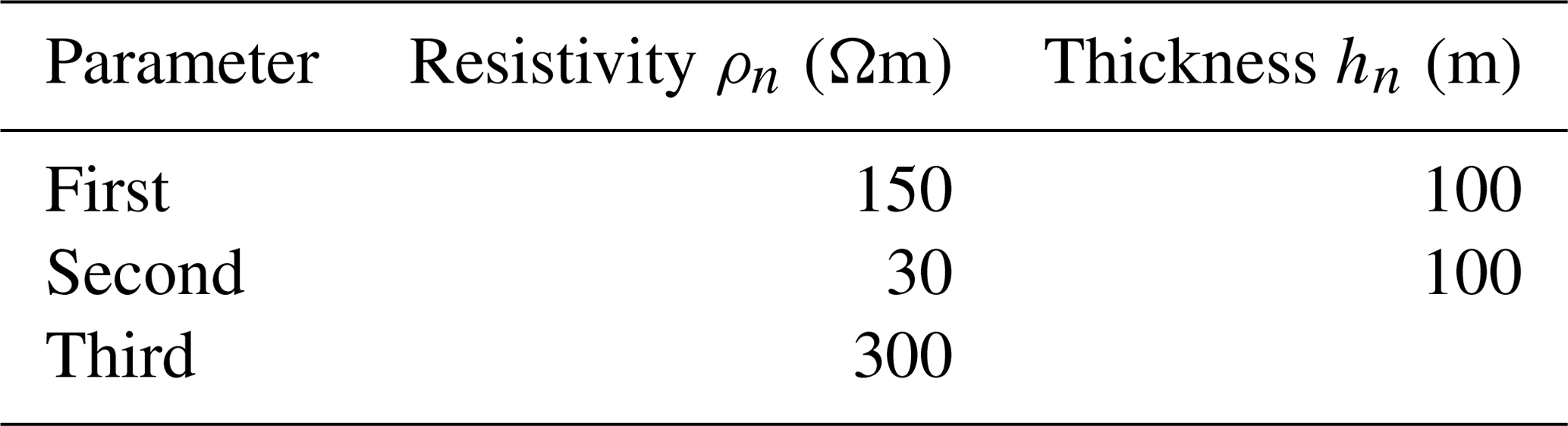
In the GREATEM system, the transmitter injects a bipolar square wave current into the ground; meanwhile the receiver and front-mounted coil were installed on an aircraft in response to the vertical component of the induced electromotive force in a horizontal layered earth model (Nabighian et al., 1988). Response signals are related to the size and depth of the underground conductor, the length and current of transmitter, the equivalent area of receiving coil, the horizontal offset, the flight altitude, and so on. These parameters can be used to calculate the time domain response as a clean signal in the horizontal layer earth model for simulation. In Fig. 1, the model parameters as follows: the length of the transmitter line TX is 1000 m on the ground, the transmitter current is 10 A with 50 % duty cycles at 25 Hz, the equivalent area of receiving coil RX is 1000 m2, the horizontal offset is 50 m, the flight altitude is 35 m, and the sample rate of the receiver is 32 kHz. In this paper, we consider a three-layer earth model where parameters are shown in Table 1. In the end, we calculated the corresponding time domain signal and the vertical response–decay curve on a three-layer earth model.
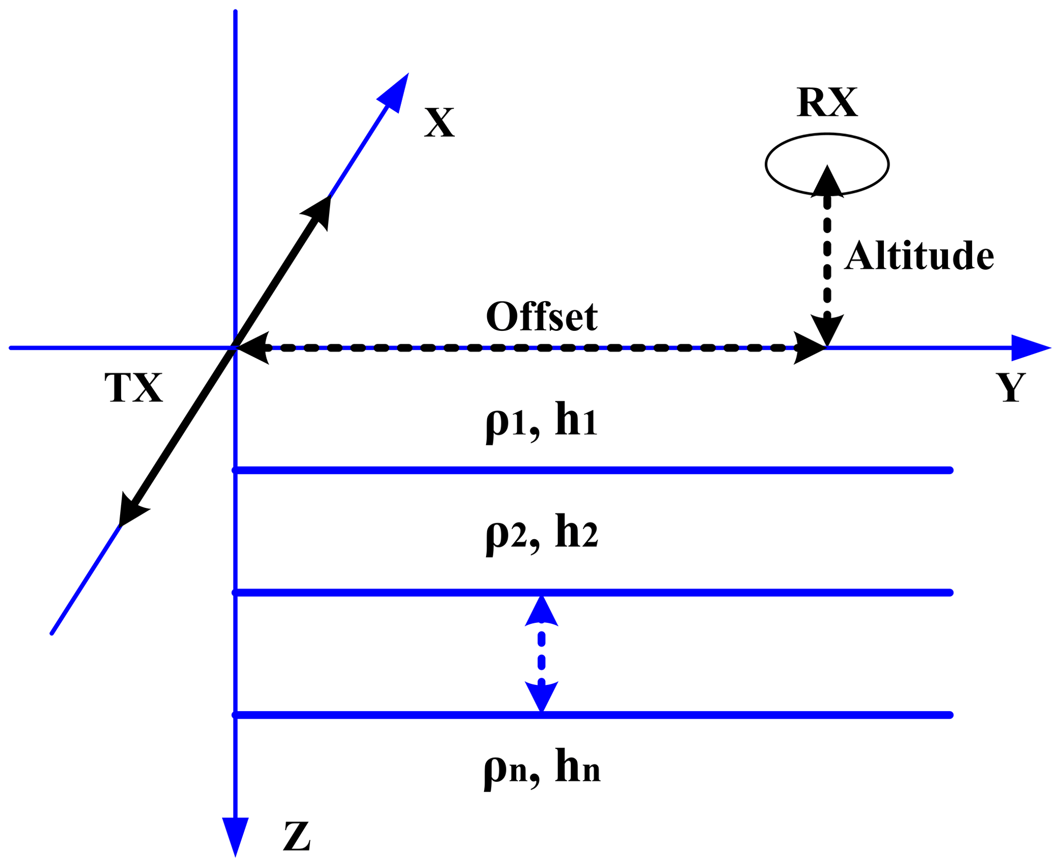
Figure 1GREATEM model based on a three-layer earth model. The TX is the transmitter line on the ground and the line length is 1000 m; the transmitter current is 10 A and the frequency is 25 Hz. The RX is the receiving coil and the equivalent area is 1000 m2; the offset is 50 m, the flight altitude is 35 m, and the sample rate of receiver is 32 kHz. The other model parameters are shown in Table 1.
Because of non-periodic and non-stationary characteristics of baseline wander, it is difficult to synthesize these noises from a simulation on the computer. The simulated signal is obtained by superimposing the clean signal on the field baseline wander measured by the inertial navigation system. Figure 2a is a simulated noisy signal which is obtained by adding baseline wander to a clean signal with the duration is 10 s. Figure 2b is the field baseline wander noise which is measured by the inertial navigation system with the duration is 10 s.
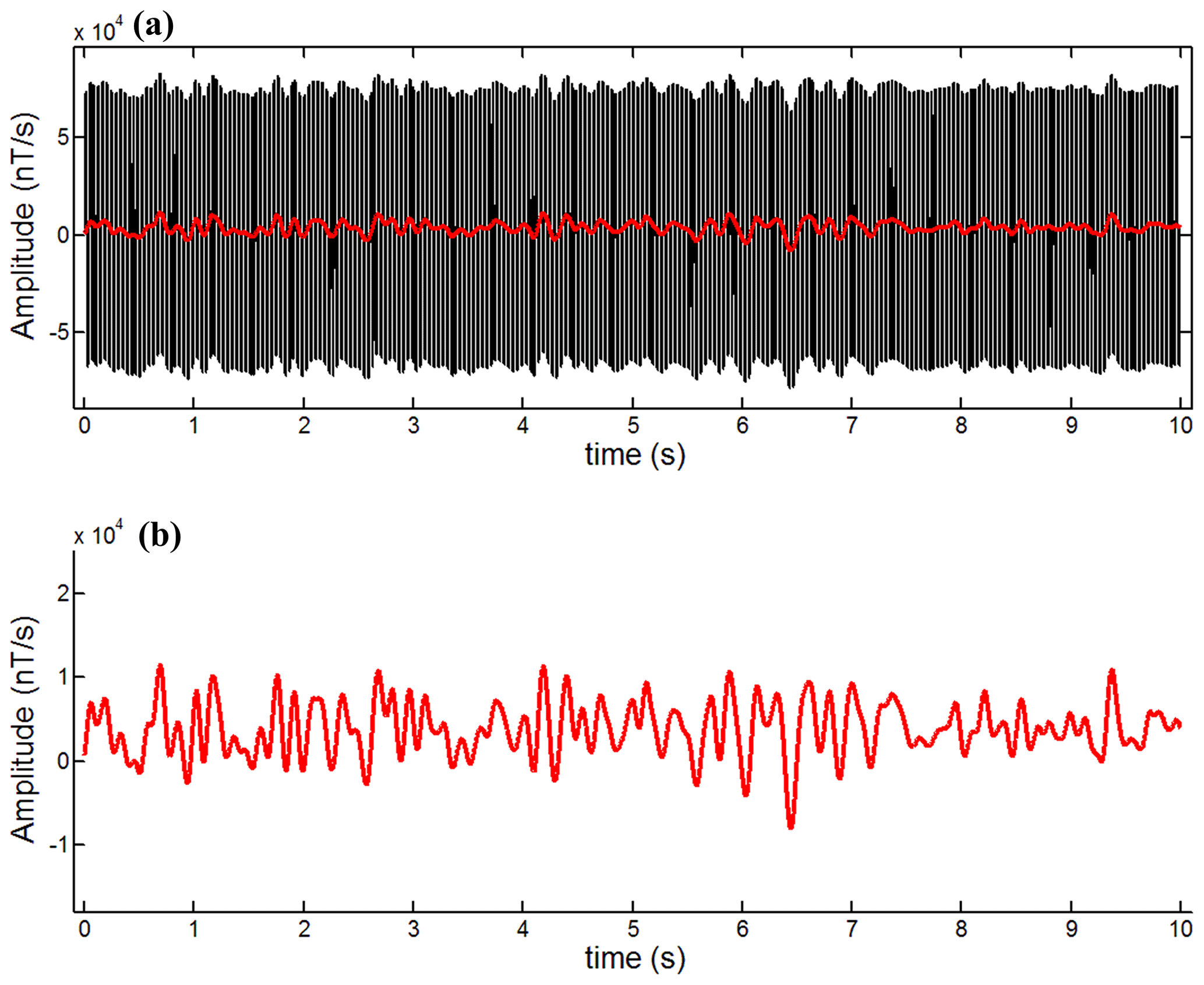
Figure 2The simulated noisy signal and baseline wander signal whose duration is 10 s. (a) The simulated noisy signals; (b) the field baseline wander measured by the inertial navigation system.
3.2 Performance of the correction and analysis
In this paper, in order to quantitatively assess the de-noised quality between our method and other methods, we propose the signal-to-noise ratio (SNR) and mean-square error (MSE) to evaluate the correctional methods in Eqs. (11) and (12), in which S(n) is a synthetic clean signal, is a de-noised signal, and L is the number of samples. The higher the SNR, the better the correctional effect; the lower the MSE, the better the fitting result.
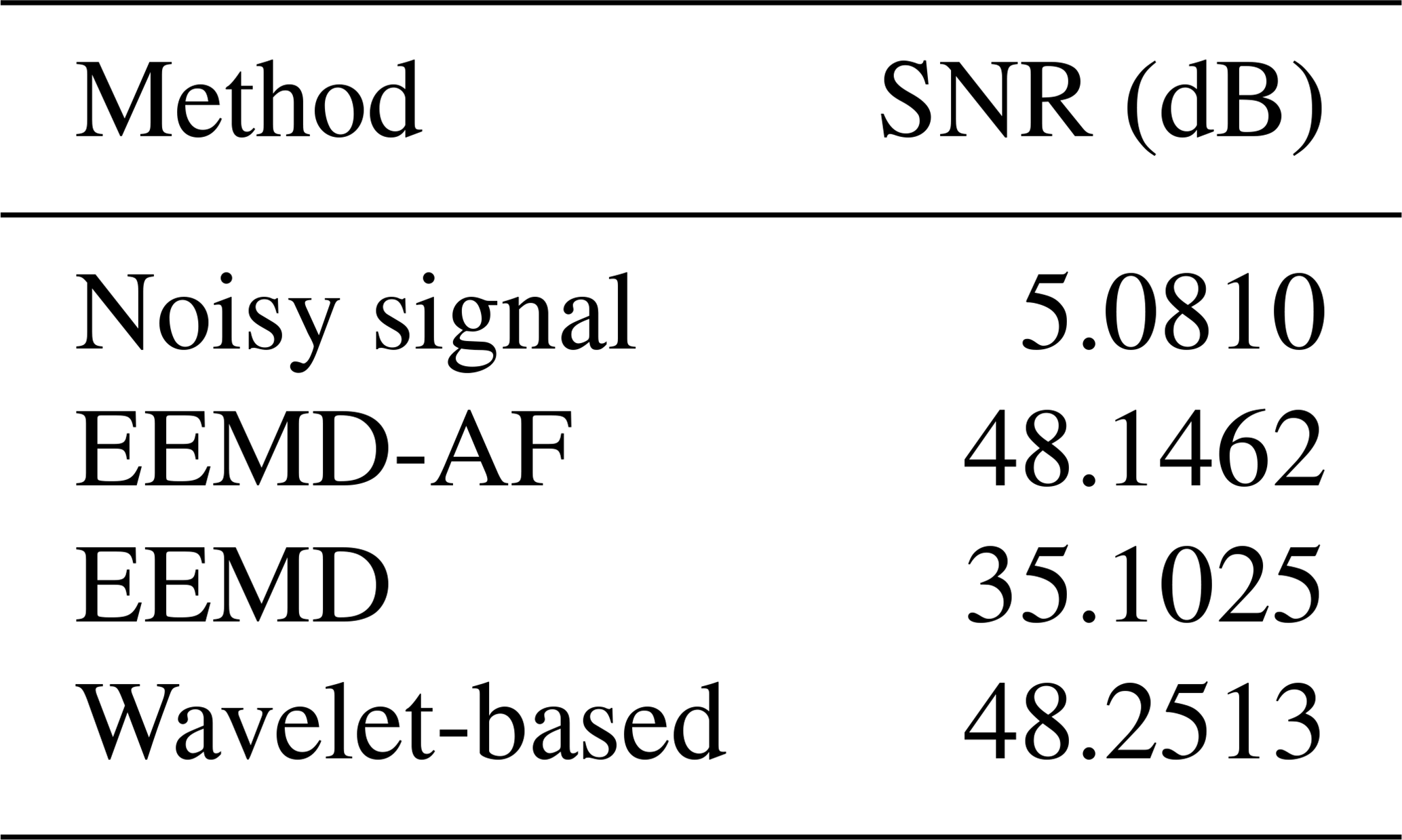
There are comparisons of SNR and MSE obtained by three correctional methods for the noisy signal whose duration is 60 s. The correctional results are shown in Table 2. In the table, the term noisy signal means the simulated noisy signal before correction. The SNR value shows that the three methods have a remarkable improvement in signal quality. It is proved that EEMD-AF and the wavelet-based method had better correctional performance than EEMD. Quantitatively, the SNR of the EEMD-AF method is significantly close to the SNR achieved by the wavelet-based method. It is obvious that the EEMD-AF achieves a correction performance similar to the wavelet-based method.
Table 2Correctional result comparison of SNR of different methods.
For further analysis, the response–decay curve is related to the conductivity of underground geological bodies in the data processing of GREATEM. Besides the SNR comparison above, the original data are used for stacking, averaging, and extracting a secondary field to build a one-by-one test point along with the survey path. Then the number of time gates is 24 per test point, where the width of time gates increases approximately logarithmically.
To generate the anomaly curve profile image, we process the simulated noisy data and correctional data by stacking, averaging, extracting, and gating. The anomaly curve profile generated from the clean signal responses is shown in Fig. 3a, where the 24 parallel lines of time gates are represented along with the test point. And Fig. 3b is an anomaly curve profile generated from the noisy signal, where the fake anomaly from Gate 14 to 24 is identified clearly due to baseline wander affecting the horizontal layer model. From Gate 20 to 24, they are mixed with each other. After the processing using the wavelet-based method, the anomaly curve profile is shown in Fig. 3c, where the fake anomaly is not accurately represented and the curves are almost parallel to each other. Figure 3d is the anomaly curve profile using the EEMD-AF method; it is obvious that the paralleled curves between the gates are better than in the above method.

Figure 3Anomaly curve profile image generated from different processed datasets. The duration of raw data is 60 s and the stacking interval is 0.2 s; therefore the number of test points is 300. (a) The clean signal from the theoretical model; (b) the noisy signal containing baseline wander; (c) the correctional signal using the wavelet-based method; (d) the correctional signal using the EEMD-AF method. The label gate marked in each panel represents the number of time gates from 1 to 24. Every specific number of a time gate means a different time width, which increased logarithmically. The vertical coordinates are changed to logarithmic format in order to facilitate the display of detail of each gate in each panel.
The comparison of SNR and MSE profiles produced by the datasets by different methods is illustrated in Fig. 4 along with the test point, where SNR and MSE of the noisy signal are marked as reference (black solid curve). In Fig. 4a, the black solid curve shows that the stacking and averaging may produce the improved SNR for a noisy signal. Quantitatively, the EEMD-AF and wavelet-based method yield an SNR which is significantly higher than the value achieved by the EEMD method. It is observed that there are fluctuations in the SNR using the wavelet-based method (red solid curve); meanwhile there are stabilities in the SNR using the EEMD-AF method (blue solid curve). And in Fig. 4b, the MSE curves indicate the same conclusion. Results from the comparison of the figures also show that the EEMD-AF method significantly outperforms the wavelet-based one for the suppression of non-stationary baseline wander.
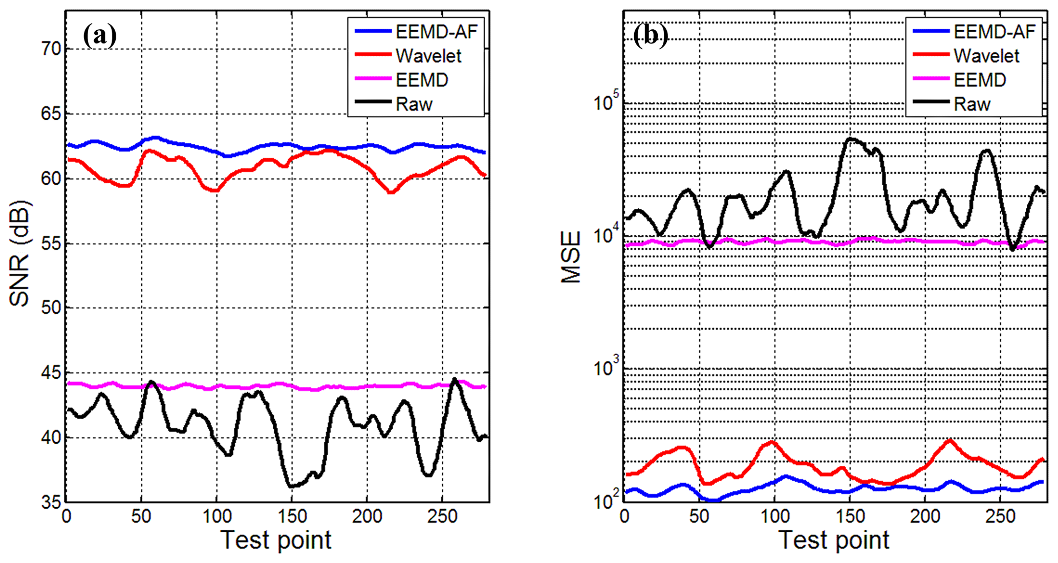
Figure 4Comparison of SNR and MSE profiles produced by the datasets by different methods along with test point. (a) The contrast between SNR on different datasets; (b) the contrast between MSE on different datasets. The vertical coordinates are changed to logarithmic format in order to show a wide range of changes in MSE.
In October 2018, a field experimental GREATEM survey was performed to detect infiltration water in the refuse landfill of Longquanyi District, Chengdu, in China. The GREATEM system was developed by Chengdu University of Technology. The electrical source transmitter was fixed on the ground; meanwhile the receiver system was mounted on the six-rotor UAV. The survey area and flight paths of the receiver were shown in Fig. 5b. The length of the transmitter line was 1100 m on the ground, the transmitter waveform was a bipolar square wave, and the current was 20 A with 50 % duty cycles at 5 Hz. The receiver system made use of 24 bit analogue-to-digital converter whose sample rate was 32 kHz, and the equivalent area of the receiving coil was 1000 m2. The transmitter line was set in the middle of flight paths and almost perpendicular to them. Each length of the flight path was 800 m, and the intervals were 80 m to each other. The flight speed of the UAV was 2.5 m s−1, and the height was 50 m from the ground.
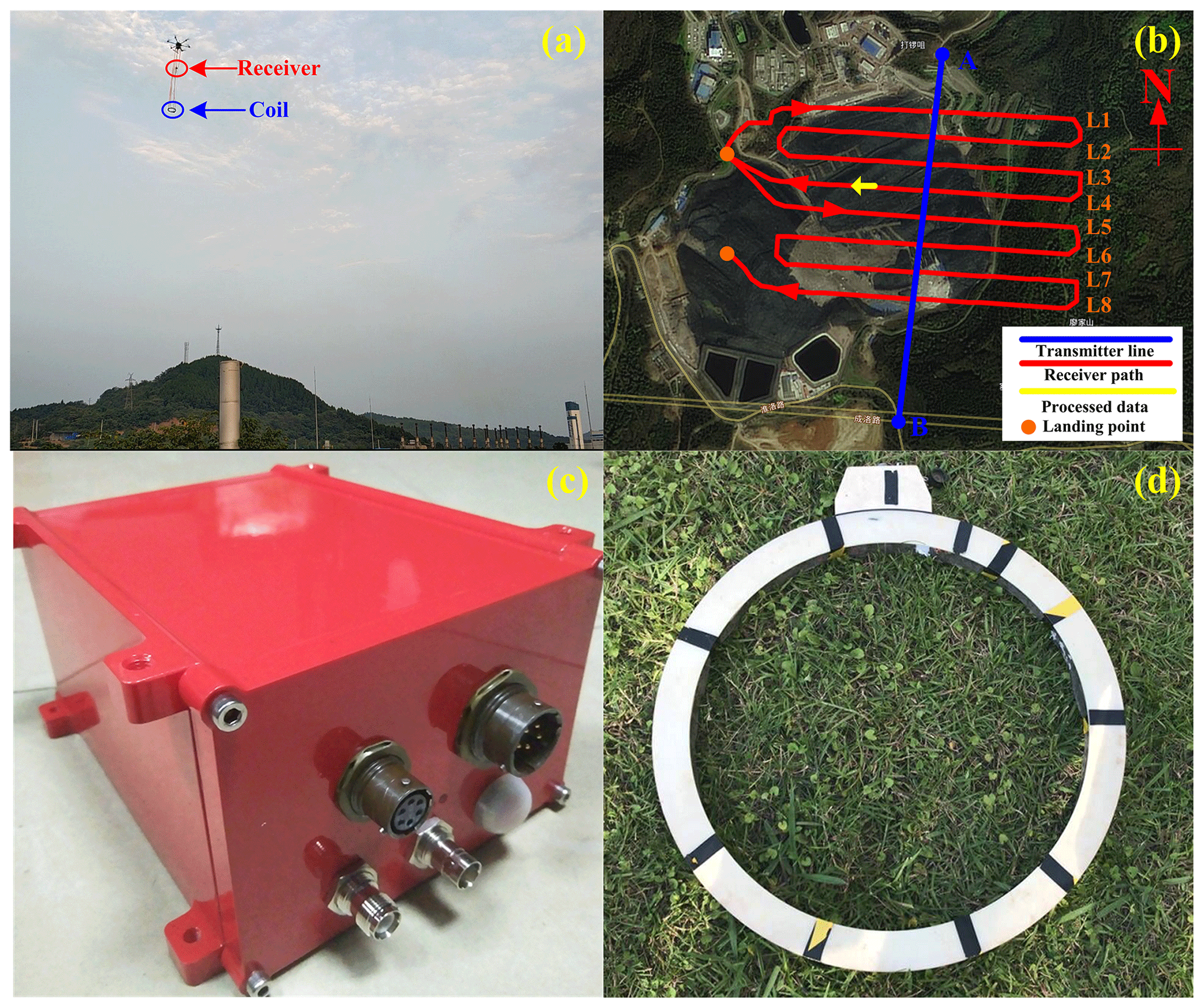
Figure 5The survey area and flight paths on the refuse landfill of Longquanyi District, Chengdu, in China. (a) The receiver system is mounted on UAV along with the paths; (b) the blue line was the transmitter source and the red curves were the survey paths of the receivers, the lines of L1 through L8 represent different paths and the orange dots represent the landing point for UAV; (c) the receiver instruments; (d) the receiving coil with a diameter of 50 cm. The flight heading was from east to west on the L4 path. The data of part of L4 (yellow arrow solid line) will be processed and the duration was 60 s. The satellite image embedded in (b) came from https://map.tianditu.gov.cn/ (last access: August 2018) built by the National Geomatics Center of China.
The amplitude of the response will decrease with the transmitter–receiver offset increase. We choose the measured data of part of the flight path L4 for our processing, and the duration of 60 s of data is shown in Fig. 6a. The baseline wander is observed to be significant on the measured data. And Fig. 6b is the correctional result from the EEMD-AF. By comparison of the signals before and after processing, the baseline wander is effectively suppressed by the EEMD-AF method.
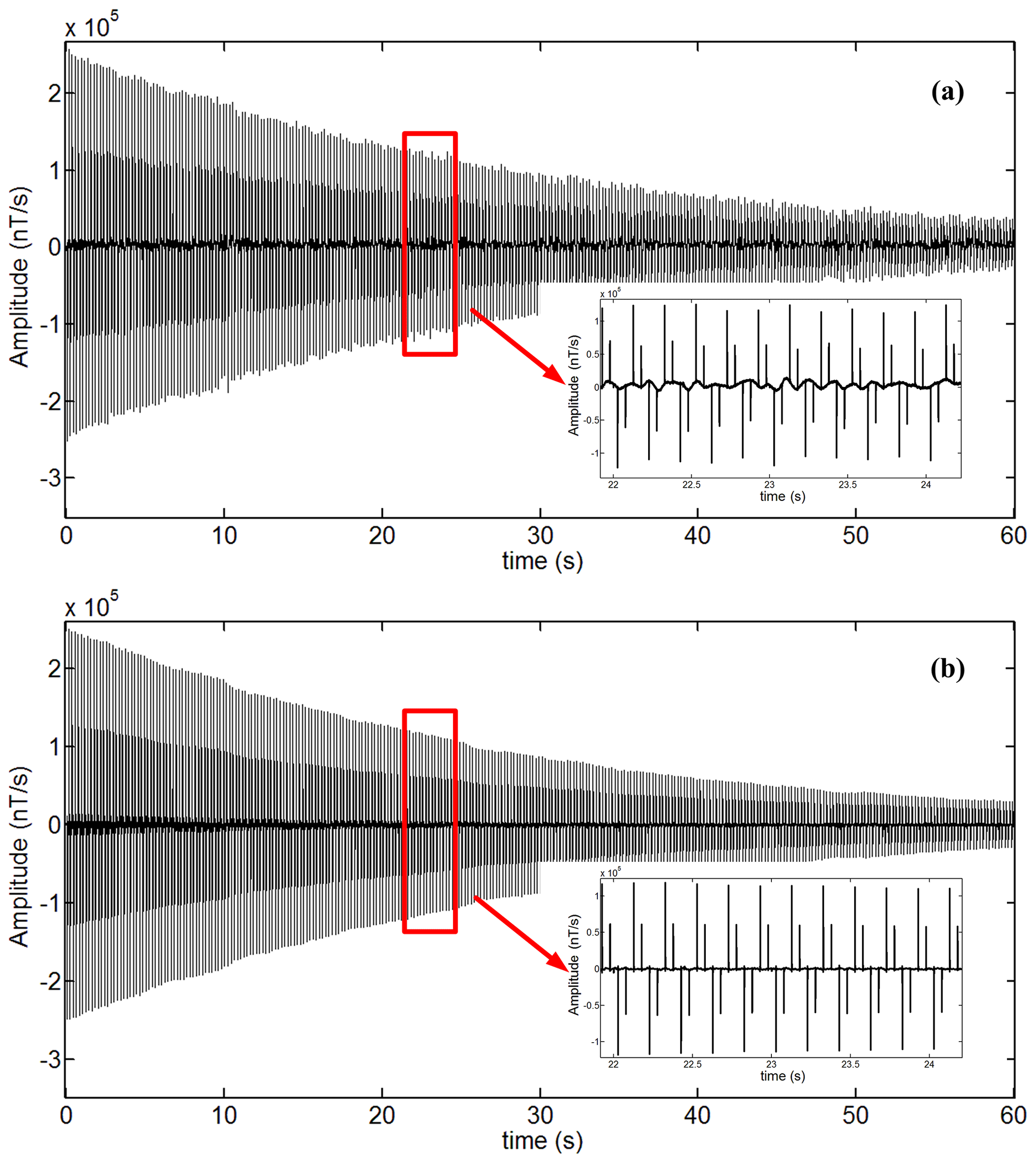
Figure 6The field data whose duration is 60 s containing baseline wander and correctional data filtered by the EEMD-AF method. (a) The field data measured by receiver instruments; (b) the correctional data using the EEMD-AF method. The data of 22 to 24 s are magnified and shown at the lower right of each panel.
Besides the comparison of the time domain data above, we produced an anomaly curve profile image from the original measured data and the correctional data, which are processed by the wavelet-based method and the EEMD-AF method respectively. The number of time gates is 18, and the widths increase approximately logarithmically per test point. Figure 7a shows the anomaly curve profile generated from the measured raw data. The correctional data using the wavelet-based and the EEMD-AF method are shown in Fig. 7b and c respectively. Based on the survey area for refuse landfill, the geological structure can be regarded as layered earth; there may be partial regions where the infiltration water was leaked.
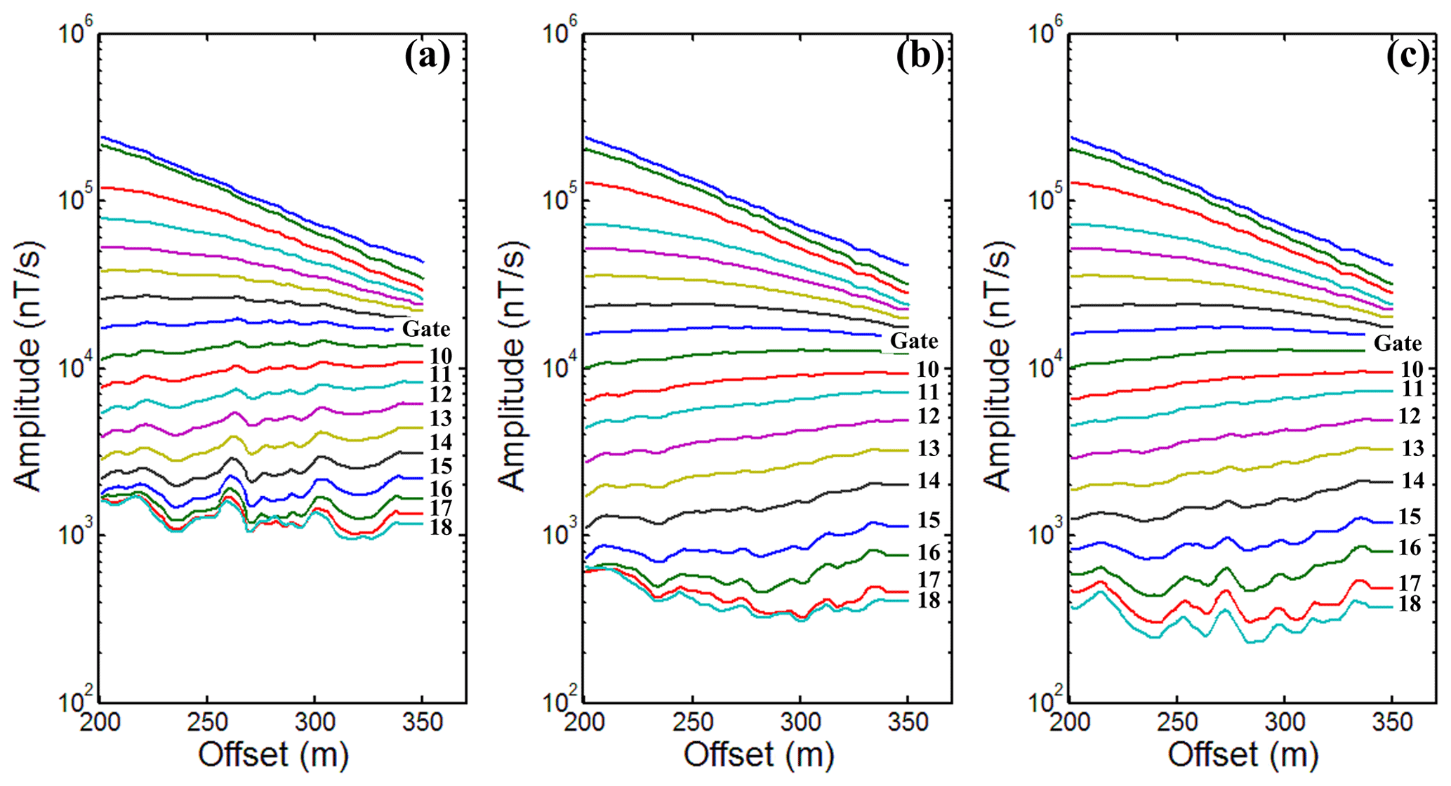
Figure 7Anomaly curve profile image generated from field data by different methods. (a) The profile of raw data; (b) the profile of data using the wavelet-based method; (c) the profile of data using the EEMD-AF method. Because the duration of raw data was 60 s and the flight speed of the UAV was 2.5 m s−1, the offset distance was 150 m. The vertical coordinates are changed to logarithmic format in order to facilitate the display of detail of each gate in each panel.
In Fig. 7a, the higher amplitude of response anomaly curves is reflected at 220, 270, and 300 m in the flight survey path. Therefore, the baseline wander exists in the original signal and affects exploration elevation and the anomaly result on inversion. The fake anomalies from Gate 10 to 15 and their interference with one another from Gate 16 to 18 are obvious. In Fig. 7b and c, after using two correction methods, the fake anomalies are suppressed on Gate 10 to 15, and their interference with one another is improved from Gate 16 to 18. In addition, Fig. 7c shows that there is no interference between the gates. However, there is partial interference on Gate 16 to 18 in Fig. 7b. By contrast with the wavelet-based method, there is no interference between the last three channels for datasets using the EEMD-AF method on an anomaly curve profile. Regarding the decay time of curves, the EEMD-AF method holds decay time 4.5 ms more than the wavelet-based method to improve the exploration elevation on the survey path. In a comparison of Fig. 7b and c, the results reveal that the performance of the EEMD-AF method is significantly superior to the wavelet-based method to suppress baseline wander. In a word, the results confirm that the EEMD-AF method is an effective and practical correctional method.
Motion-induced noise is usually referred to as baseline wander, which is an inevitable noise and always exists for the GREATEM system. The noise caused by the receiving coil motion has its own characteristics such as being low frequency, large amplitude, non-periodic, and non-stationary. This phenomenon affects the accuracy of measurements severely, leading to an inferior exploration elevation and a fake anomaly result on inversion. Therefore, we proposed the improved EEMD-AF method for baseline wander correction. The noisy signal is decomposed into N-level IMF components and a residual component by the EEMD method, and the baseline wander is generally distributed over several higher-index IMFs; then a group of adaptive low-pass filters process these IMFs successively. The baseline estimate is reconstructed by the sum of these filter output. Finally, the de-noised signal can be obtained by subtracting an estimated baseline wander from the noisy signal.
First of all, through a comparison of different de-noised methods in this paper, the SNR and MSE results show that the de-noised performance of the EEMD-AF method is significantly superior to the other methods. And the same conclusion can be reached from the anomaly curve profile image. Furthermore, in field data processing, the baseline wander is effectively suppressed by EEMD-AF and the wavelet-based method. Because there is no interference between the last few gates, the comparison of the anomaly curve profile image reveals that the EEMD-AF method is significantly better than the wavelet-based method. These results also indicate that the EEMD-AF method is a practical as well as an effective method for the suppression of the baseline wander in the GREATEM signal.
In this paper, the data are not publicly accessible because funder terms require the original geological data to be kept confidential without cooperative licensing agreements.
First, YL and SG designed the method model and developed the code. Second, the author SZ designed the field experiments and carried them out with HH and PX on the survey area. Third, YL and CY performed the simulations and processed data. Finally, YL prepared the paper with contributions from all co-authors.
The authors declare that they have no conflict of interest.
The authors thank the members of the project committee for their help. We also acknowledge the referees and the editor for their constructive remarks and suggestions.
This research has been supported by the “Research on fixed wing time domain airborne electromagnetic measurement technology system (grant no. 2017YFC0601900)”.
This paper was edited by Luis Vazquez and reviewed by two anonymous referees.
Bouchedda, A., Chouteau, M., Keating, P., and Smith, R.: Sferics noise reduction in time-domain electromagnetic systems: application to MegaTEM II signal enhancement, Explor. Geophys., 41, 225–239, https://doi.org/10.1071/EG09007, 2010.
Buselli, G., Hwang, H. S., and Pik, P. J.: AEM noise reduction with remote referencing, Explor. Geophys., 29, 71–76, https://doi.org/10.1071/EG998071, 1998.
Flandrin, P., Goncalves, P., and Rilling, G.: Detrending and denoising with empirical mode decomposition, 12th European Signal Processing Conference, Vienna, Austria, September 2004.
Liu, F., Li, J., Liu, L., Huang, L., and Fang, G.: Application of the EEMD method for distinction and suppression of motion-induced noise in grounded electrical source airborne TEM system, J. Appl. Geophys., 139, 109–116, https://doi.org/10.1016/j.jappgeo.2017.02.013, 2017.
Huang, N. E., Shen, Z., Long, S. R., Wu, M. C., Shin, H. H., Zheng, Q., Yen, N. C., Tung, C. C., and Liu, H. H.: The Empirical Mode Decomposition and the Hilbert spectrum for nonlinear and non-stationary time series analysis, P. R. Soc. Lond. A, 454, 903–995, https://doi.org/10.1098/rspa.1998.0193, 1998.
Lemire, D.: Baseline asymmetry, Tau projection, B-field estimation and automatic halfcycle rejection, Technical Report, THEM Geophysics Inc., PhD, THEM Geophysics Inc, Canada, 13 pp., 2001.
Macnae, J. C., Lamontagne, Y., and West, G. F.: Noise processing techniques for time-domain EM system, Geophysics, 49, 934–948, https://doi.org/10.1190/1.1826986, 1984.
Mogi, T., Tanaka, Y., Kusunoki, K., Morikawa, T., and Jomori, N.: Development of grounded electrical source airborne transient EM(GREATEM), Explor. Geophys., 29, 61–64, https://doi.org/10.1071/EG998061, 1998.
Nabighian, M. N.: Electromagnetic methods in applied geophysics, Volume 1: Theory, Society of Exploration Geophysicists Publications, United Kingdom, 1988.
Smith, R. S., Annan, A. P., and McGowan, P. D.: A comparison of data from airborne, semi-airborne and ground electromagnetic systems, Geophysics, 66, 1379-1385, https://doi.org/10.1190/1.1487084, 2001.
Wang, Y., Ji, Y., Li, S., Lin, J., Zhou, F., and Yang, G.: A wavelet-based baseline drift correction method for grounded electrical source airborne transient electromagnetic signals, Explor. Geophys., 44, 229–237, https://doi.org/10.1071/EG12078, 2013.
Wu, Z. and Huang, N. E.: Ensemble empirical mode decomposition: a noise-assisted data analysis method, Adv. Adapt. Data Anal., 1, 1–41, https://doi.org/10.1142/S1793536909000047, 2009.