
Abstract
Space charge dynamics under AC stress is of importance as a majority of high voltage cables are under AC stress, and space charge is the driving mechanism of dielectric degradation under these conditions. Bipolar charge transport model is used to simulate space charge dynamics in polyethylene under AC stress. The current density, electroluminescence intensity and space charge density under sinusoidal, triangular and square voltages are compared. It is found that there is no phase shift between current density, electroluminescence intensity and applied voltages, which disagrees the results of Baudoin et al. The thickness of space charge layer under AC stress is much thinner that under DC stress.
Export citation and abstract BibTeX RIS

Original content from this work may be used under the terms of the Creative Commons Attribution 4.0 licence. Any further distribution of this work must maintain attribution to the author(s) and the title of the work, journal citation and DOI.
1. Introdution
Polyethylene is the preferred insulation material of high voltage cables. However, polyethylene may suffer chemical and physical degradation after long-standing operation. It is generally believed that the space charge accumulation plays an important role in dielectric degradation [1].
Most efforts have been expended in studying space charge characteristics in polyethylene under DC stress, while there is comparatively much less attempts to investigate space charge characteristics under AC stress [2–7]. The possible reason for the limited research is not the lack of interest for having information on space charge characteristics under AC stress, for a majority of high voltage cables are under AC stress and space charge is the driving mechanism of dielectric degradation. Space charge can distort the local electric field, and cause partial discharge and electrical tree growth. In addition, the trapped charges change the chemical reactivity of charged centers. Actually, the reason is that the quite small quantity and thin thickness of space charge layer under AC stress make measurement and simulation difficult.
Zhao et al have developed a bipolar charge transport model to simulate space charge in polymers under AC electric field with different amplitude and frequency [8]. Baudoin et al have proposed a bipolar charge transport model allowing the description of electroluminescence in polyethylene under AC stress and tested by comparing simulated and experimental electroluminescence patterns [9]. However, the simulated charge density and current density is larger than those under DC stress with the same electric field amplitude, which disagrees with the experimental results. Thomas et al have obtained space charge profiles in polyethylene under sinusoidal or square AC stress using the modified pulsed electro-acoustic system [10].
The paper is organized as follows. The bipolar charge transport model and numerical scheme is introduced in section 2. The space charge characteristics under sinusoidal, triangular and square waveforms are presented in section 3. The paper concludes in section 4 with a summary of the key results.
2. Bipolar charge transport model
2.1. Sets of equations
The bipolar charge transport model is based on bipolar charge injection, transport as well as recombination of opposite charges. The charge carrier dynamics can be described by the following equations [2, 9]:


where n is the number densities, j is the current density, e is the electron charge, s is the source term resulting from recombination processes, μ is the mobility, E is the electric field, ε is the permittivity (2.3 for polyethylene). The subscript 'e' and 'h' refer to the electrons and holes, respectively. The superscript 'f' refers to the mobile carriers. By assuming that there is an exponential distribution of the trap density and the temperature T is much less than the shape parameter T0(e,h) , the density of mobile carriers can be approximated by

The source term can be expressed as

where S1 and S2 are the recombination coefficients for mobile electrons-trapped holes and trapped electrons-mobile holes, respectively.
Based on the hopping mechanism of charge transport in polyethylene, the mobility has the form


Where ν is the frequency of escape (6.2 × 10¹² s−1 at room temperature), Δf is the upper filled level, Δm is the maximum trap depth, N' is the pre-exponential factor of the trap density distribution, T0 is the shape parameter, d(e,h) is the average distance between electron or hole traps.
An injection flux based on Schottky law is of the form


for electrons at cathode and holes at anode. A = 1.2 × 10⁶ Am−2K−2 is the Richardson constant, kB is the Boltzmann constant, wei and whi are injection barrier for electrons and holes, d is the dielectric thickness.
The extraction fluxes are of the form


for electrons at anode and holes at cathode.
A sinusoidal, triangular or square alternating voltage is applied to the anode (x = d), and at the cathode (x = 0) the potential is set to zero. The conduction current density is

Note that the displacement current is not discussed here.
As the spaced average combination rate is proportional to the electroluminescence intensity, the electroluminescence intensity can be defined by

Sets of parameters appear suitable to describe space charge dynamics under DC stress [2]. Almost the same parameters are adopted for AC conditions except for the lower initial charge density and the mobility. Parameters used in the model are shown in table 1.
Table 1. Parameter used in the model.
| Symbol | Parameter | Value |
|---|---|---|
| S1 | recombination rate between mobile electrons and trapped holes | 1.6 × 10⁻²¹ m3s−1 |
| S2 | recombination rate between trapped electrons and mobile holes | 1.6 × 10⁻²¹ m3s−1 |
| Δme | electron maximum trap depth | 0.67 eV |
| Δmh | hole maximum trap depth | 0.67 eV |
| T0e | electron shape parameter | 104 K |
| T0h | hole shape parameter | 104 K |
| N'e | electron pre-exponential factor | 1047 m−3J−1 |
| N'h | hole pre-exponential factor | 1047 m−3J−1 |
| wei | electron injection barrier | 1.27 eV |
| whi | hole injection barrier | 1.16 eV |
| ρe (t = 0) | initial charge density of electron | −1.6 × 10⁻¹¹ Cm−3 |
| ρh (t = 0) | initial charge density of hole | 1.6 × 10⁻¹¹ Cm−3 |
2.2. Numerical scheme
The domain of calculation is divided into 2000 elements, of vary lengths for 100 μm thick polyethylene thin film: 50 elements within a distance of 10 nm from the electrode, 90 elements at the distance of 10 nm ∼ 100 nm, 180 elements at the distance of 100 nm ∼ 1 μm, 360 elements at the distance of 1 μm ∼ 10 μm, and 640 elements at the distance of 10 μm ∼ 90 μm from the cathode. It is noted that it is necessary to use variable space discretization, because space charge layer thickness is much thinner compared with those under DC stress. The time step Δt is chosen to satisfy the Courant-Friedrichs-Lewy condition whose typical value is 2.0 × 10⁻⁵ s. As the continuity equation (1) is the convection dominated convection–diffusion equation, accurate numerical algorithm without under- and overshoot is vital for reproducing charge dynamics in polyethylene. Three-order flux limiter is adopted to achieve better accuracy than first-order upwind, as well as positivity without introducing numerical diffusion or oscillation, which is described in detail in [2].
3. Results and discussions
3.1. Current density
Square, triangular or sinusoidal voltage is applied to the anode, as shown in figure 1. Numerical simulations are performed for a stress time of 5 s. The amplitude and frequency of all three waveforms are 6 kV and 50 Hz, respectively. Current density under sinusoidal waveform is shown in figure 2. It can be seen that the phase difference between applied voltage and current density is 180°. The reason is that when the applied voltage is positive, the direction of electron drift is along the positive x direction, and current density is negative. The maximum current density is about 1.1 × 10⁻²⁰ A m−2, which disagrees with the results of Baudoin et al [9]. The maximum current density of Baudoin et al is about 1.7 × 10⁻¹ A m−2. When the initial charge density is 0.5 Cm−3 and 60 kV mm−1 DC electric field is applied, the current density is 1.3 × 10⁻⁹ A m−2, which agrees with the experimental results [2]. It can be inferred that the current density of Baudoin et al far exceeds the actual values.
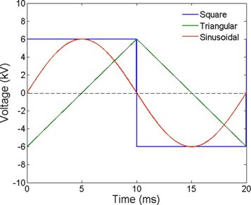
Figure 1. AC voltage applied to the anode.
Download figure:
Standard image High-resolution image
Figure 2. Current density under sinusoidal waveform.
Download figure:
Standard image High-resolution imageCurrent densities under square, triangular or sinusoidal voltages are shown in figure 3. It can be seen that the frequency and the maximum of three current densities are the same, and the phase differences between current densities and applied voltages are all 180°.
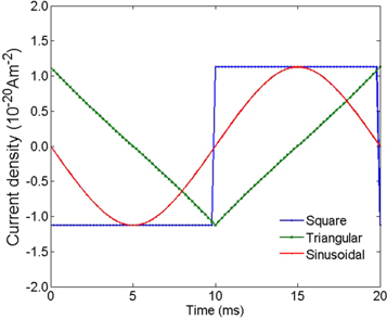
Figure 3. Comparison of current density under different waveforms.
Download figure:
Standard image High-resolution image3.2. Electroluminescence
Electroluminescence intensity under sinusoidal waveform is shown in figure 4. It can be seen that electroluminescence intensity reaches its peak when the applied voltage reaches its positive and negative peak, while electroluminescence intensity reaches its minimum value when the applied voltage reaches zero. It is noted that there is no much difference between the maximum and minimum of the electroluminescence intensity.
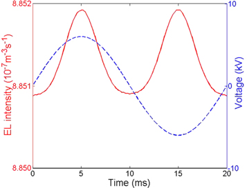
Figure 4. Electroluminescence intensity under sinusoidal waveform.
Download figure:
Standard image High-resolution imageElectroluminescence intensities under square, triangular or sinusoidal voltages are shown in figure 5. It can be seen that there is much difference between electroluminescence intensities under different waveforms. Electroluminescence intensity under square voltage is almost straight, and electroluminescence intensity under sinusoidal voltage is almost 100 Hz sinusoidal waveform. However, electroluminescence intensity under triangular voltage appears the bathtub-shaped. Electroluminescence intensity decreases relatively rapidly, and increases much more slowly, which agrees the results of Baudoin et al [9].
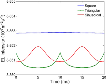
Figure 5. Comparison of electroluminescence intensity under different waveforms.
Download figure:
Standard image High-resolution image3.3. Space charge density
Space charge density under sinusoidal waveform is shown in figure 6. It can be seen that the distribution of total electrons and mobile electrons is similar, and the distribution of total holes and mobile holes is similar. The reason is that mobile carrier densities are approximated by formula (4). Electron and hole densities reach the maximum at t = 5 ms and t = 15 ms. The maximum electron and hole densities are 1.4 × 10⁸ m−3 and 1.1 × 10⁹ m−3, respectively. This is because that electron injection barrier is larger than hole injection barrier as shown in table 1, so more holes are injected from the anode. The charge layer thickness is about 0.18 ∼ 0.30 nm from the electrode, which agrees with the results of Baudoin et al in magnitude. It is hereby certified that variable space discretization, being tightened close to the electrodes is essential to achieve enough spatial resolution of space charge dynamics.
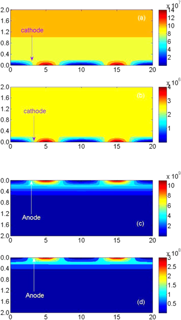
Figure 6. Space charge density under sinusoidal waveform. (a) total electrons, (b) mobile electrons, (c) total holes and (d) mobile holes.
Download figure:
Standard image High-resolution imageSpace charge density under triangular waveform is shown in figure 7. It can be seen from figure 7 that electron and hole densities reach the maximum at t = 0 ms, t = 10 ms and t = 20 ms. The maximum electron and hole densities under triangular voltage are the same as those under sinusoidal voltage. However, high carrier densities under triangular voltage last shorter than those under sinusoidal voltage.

Figure 7. Space charge density under triangular waveform. (a) total electrons, (b) mobile electrons, (c) total holes and (d) mobile holes.
Download figure:
Standard image High-resolution imageSpace charge density under square waveform is shown in figure 8. It can be seen from figure 8 that carrier distribution under square voltage is quite different from that under sinusoidal and triangular voltage. The carrier distribution at the same distance from the electrodes is approximately the same. When the voltage polarity reversal at the anode occurs, the carrier distribution changes little. The reason is that the characteristic time to redistribute charge carriers is the order of several seconds. When square voltage with 50 Hz frequency is applied, the time interval of 10 ms is not enough to redistribute charge carriers. The charge layer thickness under square voltage is a little larger than that under sinusoidal or triangular voltage.

Figure 8. Space charge density under square waveform. (a) total electrons, (b) mobile electrons, (c) total holes and (d) mobile holes.
Download figure:
Standard image High-resolution image
4. Conclusion
Bipolar charge transport model is used to simulate space charge dynamics in polyethylene under AC stress. We compare the current density, electroluminescence intensity and space charge density under sinusoidal, triangular and square voltage with 6 kV amplitude and 50 Hz frequency. It is found that the phase differences between current densities and applied voltages are all 180°. There is no phase shift between electroluminescence intensity and applied voltages. The thickness of space charge layer under AC stress is much thinner than that under DC stress with the same amplitude.
Acknowledgments
The work was supported by the Chinese National Natural Science Foundation under the Grant 51677024, Program for Innovative Talents in University of Liaoning Province under the Grant LR2019047, and Natural Science Foundation of Liaoning Province under the Grant 2020-MS-214.
Data Availability
The data that support the findings of this study are available from the corresponding author upon reasonable request.