2.1 Field study

Silt loam soil Albic Luvisol from arable cropland of Merklingsen experimental station located near Soest (North Rhine-Westphalia, Germany; 51^∘34^′15.5^′′ N, 8^∘00^′06.8^′′ E) was used (87 % silt, 11 % clay, 2 % sand). The soil density of intact cores was 1.3 g mL⁻¹, pH value was 6.8, total C content was 1.30 %, total N content was 0.16 %, and organic matter content was 2.14 %. The field was sown with winter rye in September 2015 and mineral underfoot fertilization was applied. Our experiments were conducted on experimental plots of a field study on management effects on greenhouse gas fluxes. We selected the “climate-optimized farm” treatment where a complex cropping rotation of silage maize, winter wheat, faba bean, winter barley, and perennial rye had been established since 2010 (Kramps-Alpmann et al., 2017). This treatment was managed by zero tillage with direct seeding, and fertilization was a combination of organic (biogas digestate) and mineral fertilizer where doses were set according to official fertilizer recommendations (Baumgärtel and Benke, 2009). On 13 October in each of the four replicate plots (6 m×12 m), we established microplots consisting of aluminum cylinders (length 35 cm, diameter 15 cm) inserted to 30 cm depth into the soil so that 5 cm extended above the ground for installation of the flux chamber. Three field campaigns were carried out in November 2015 (F1), March 2016 (F2), and May/June 2016 (F3). After each field campaign the cylinders were removed, cleaned, and later reinstalled at new locations (on 27 November 2015 for F2 sampling and on 28 April 2016 for F3 sampling) for the next field campaign.

On each replicate plot, cylinders were installed pairwise – one for gas-flux measurements and one for mineral nitrogen sampling – for three treatments – natural abundance (NA), traced nitrate (${}^{\mathrm{15}}{\mathrm{NO}}_{\mathrm{3}}^{-}$), and traced ammonium (${}^{\mathrm{15}}{\mathrm{NH}}_{\mathrm{4}}^{+}$) – which is in total six cylinders per replicate plot. The distance between each treatment cylinder was at least 2 m; the pair of cylinders for one treatment were separated by 0.5 m distance.

At the beginning of the experiment, a fertilizer solution with 240 mg N L⁻¹ as NaNO₃ and 240 mg N L⁻¹ as NH₄Cl was added to the experimental microplots with the needle injection technique. Three milliliters of the fertilizer solution was injected into 72 points using 12 needles inserted subsequently into six depths (2.5, 7.5, 12.5, 17.5, 22.5, and 27.5 cm) from the top to the bottom using peristaltic pump. This strategy was based on previous studies (Buchen et al., 2016; Wu et al., 2011) and was enhanced by pre-experimental tests to obtain the most homogeneous tracer distribution (Lewicka-Szczebak and Well, 2020). Total fertilization was 20 mg N per kg soil (added as NaNO₃ (10 mg N) and NH₄Cl (10 mg N)), which was equivalent to about 80 kg N ha⁻¹.

In total, 216 mL of fertilizing solution was inserted into each microplot, which resulted in a 3 % increase in water content. For ¹⁵N-labeled treatments, the ¹⁵N content in fertilizing solution was calculated to achieve about 60 at. % (atomic percent) ¹⁵N in the ¹⁵N-labeled N pool. The ${}^{\mathrm{15}}{\mathrm{NO}}_{\mathrm{3}}^{-}$ treatment received tracer solution containing 68 at. % ¹⁵N, and the ${}^{\mathrm{15}}{\mathrm{NH}}_{\mathrm{4}}^{+}$ treatment received 64 at. % ¹⁵N.

Immediately after fertilizing solution addition, the flux chamber microplots were closed for gas accumulation. Opaque PVC chambers of an area of 1.767 dm² and a volume of 2.65 dm³ were applied with installed valves for sample collection and a fan for gas mixing. The closed chamber method (Hutchinson and Mosier, 1981) was used for N₂O flux measurement. Chambers were closed and sealed with airtight rubber bands for 120 min, and headspace sampling was performed after 40, 80 and 120 min into evacuated crimped 20 mL vials with a 30 mL syringe for gas-flux measurements. Additionally, after 120 min, samples for isotope analysis were collected. For ¹⁵N treatments, two identical replicates were taken into 12 mL evacuated screw-cap Exetainers^® (Labco Limited, Ceredigion, UK) with two combined 15 mL syringes. For the NA treatment, one gas sample was transferred into an evacuated 115 mL crimp-cap vial with a 150 mL syringe.

Each field campaign lasted 5 d. Gas samples were collected once on the first day after fertilization, afterwards twice a day – in the morning and in the evening, and once on the last 5th day in the morning.

The soil sampling microplots were treated identically and used for mineral nitrogen sampling. The soil samples were collected with a Goettinger boring rod with 18 mm outer diameter and 14 mm slots (Nietfeld GmbH, Quakenbrück, Germany). Boreholes were sealed by inserting a closed sand-filled PVC pipe with the same diameter as the bore. For each sampling, three cores were collected and homogenized to one mixed sample each day; hence, we performed five soil samplings during each campaign. The samples were immediately transported to the laboratory at 6 ^∘C, and mineral nitrogen extractions were performed on the same day.

2.2 Laboratory incubation

The soil from the experimental field site was used to prepare incubation columns for laboratory incubation. The soil, upper 30 cm layer, was collected on the 18 January 2018 from the experimental plot used previously for field campaigns, and the incubation was conducted from 19 February 2018 to 5 March 2018. The soil was air-dried and sieved at 4 mm mesh size. Afterwards, the soil was rewetted to achieve a water content equivalent to 60 % water-filled pore space (WFPS) and fertilized with 20 mg N per kg soil, added as NaNO₃ (10 mg N) and NH₄Cl (10 mg N). Analogically as in the field study, three treatments were prepared: natural abundance (NA), labeled with ¹⁵N nitrate (¹⁵NO₃), and labeled with ¹⁵N ammonium (¹⁵NH₄). For the ¹⁵NO₃ treatment, NaNO₃ solution with 72 at. % ¹⁵N was added, and for the ¹⁵NH₄ treatment, NH₄Cl solution with 63 at. % ¹⁵N was added. Then soils were thoroughly mixed to obtain a homogenous distribution of water and fertilizer and an equivalent of 1.69 kg dry soil was repacked into each incubation column with a bulk density of 1.3 g cm⁻³.

For each treatment, 14 columns were prepared, and half of them received additional water injected into the top of the column (100 mL water added) to prepare two moisture treatments: dry (61 % WFPS) and wet (72 % WFPS). The incubation lasted 12 d. In the meantime, on the 6th day of incubation, water addition on the top of each column was repeated (80 mL water added) to increase the soil moisture in both treatments to ca. 68 % WFPS in the dry treatment and ca. 81 % WFPS in the wet treatment. The WFPS values were controlled during the experiment (Fig. S1 in the Supplement). The strategy of adding water on the top of the column to achieve target water content was necessary to allow for mixing and compaction at a suitable (low) water content of the soil and thus to optimize homogeneity of water and fertilizer distribution (Lewicka-Szczebak and Well, 2020). The incubation temperature was 20 ^∘C. The columns were continuously flushed with a gas mixture with reduced N₂ content to increase the measurement sensitivity (2 % N₂ and 21 % O₂ in He; Lewicka-Szczebak et al., 2017) with a flow of 9 mL min⁻¹. Gas samples were collected daily into two 12 mL septum-capped Exetainers^® (Labco Limited, Ceredigion, UK) and one crimped 100 mL vial connected to the vents of the incubation columns. Soil samples were collected five times during the incubation by sacrificing one incubation column per sampling event, which was then divided into three subsamples (replicate samples of mixed soil).

2.3 Gas analyses

Measurements of N₂O concentrations in the 20 mL samples were carried out with a gas chromatograph (GC-2014, Shimadzu, Duisburg, Germany) equipped with an electron capture detector (ECD) and an autosampler (Loftfields Analytical Solutions, Neu Eichenberg, Germany). The analytical precision was around 2 %.

Flux rates of total N₂O for field campaigns, i.e., including fluxes from ¹⁵N-labeled and nonlabeled sources, were calculated from ordinary linear regression of the four consecutive samples over time using the R package gasfluxes (Fuß, 2015) and the following equation:

where $J_{{\mathrm{N}}_{\mathrm{2}}\mathrm{O}}$ is the flux rate (in µg N₂O-N ${\mathrm{m}}^{-\mathrm{2}}{\mathrm{h}}^{-\mathrm{1}}$), $C_{{\mathrm{N}}_{\mathrm{2}}\mathrm{O}}$ is N₂O mass concentration (in µg N m⁻³) corrected by the chamber temperature according to the ideal gas law, t is closing time of the chamber, V is volume of the chamber (in m³), and A is covered soil area (in m²).

For laboratory incubations, fluxes were calculated based on the dynamic chamber principle. Correction for the inlet concentration is omitted since the N₂O-free gas mixture was used for flushing:

where $J_{{\mathrm{N}}_{\mathrm{2}}\mathrm{O}}$ is the flux rate (in µg N₂O-N ${\mathrm{m}}^{-\mathrm{2}}{\mathrm{h}}^{-\mathrm{1}}$), C is N₂O mass concentration (in µg N m⁻³) corrected by the incubation temperature according to the ideal gas law, Q is the gas flow rate through the incubation vessels (in m³ h⁻¹), and A is soil area in the incubation vessel (in m²).

The gas samples collected from ¹⁵N treatments were analyzed for ¹⁵N content with a modified GasBench II preparation system coupled to MAT 253 isotope ratio mass spectrometer (Thermo Scientific, Bremen, Germany) according to Lewicka-Szczebak et al. (2013). In this setup, N₂O is converted to N₂ during in-line reduction, and stable isotope ratios ²⁹R (²⁹N₂∕²⁸N₂) and ³⁰R (³⁰N₂∕²⁸N₂), of N₂, of the sum of denitrification products (N₂+N₂O) and of N₂O are determined. Based on these measurements, the following values are calculated according to the respective equations (after Spott et al., 2006):

The ¹⁵N abundance of the ¹⁵N-labeled pool (a_P) from which N₂ ($a_{{\text{P\_N}}_{\mathrm{2}}}$) or N₂O ($a_{\text{P\_}{\mathrm{N}}_{\mathrm{2}}\mathrm{O}}$) originates is calculated as follows:

The calculation of a_P is based on the nonrandom distribution of N₂ and N₂O isotopologues (Spott et al., 2006), where ³⁰x_M is the fraction of ³⁰N₂ in the total gas mixture,

a_M is ¹⁵N abundance in total gas mixture,

and a_bgd is ¹⁵N abundance of the nonlabeled pool (atmospheric background or experimental matrix).

The fraction originating from the ¹⁵N-labeled pool (f_P) for N₂ ($f_{{\text{P\_N}}_{\mathrm{2}}}$), N₂+N₂O ($f_{\text{P\_}{\mathrm{N}}_{\mathrm{2}}+{\mathrm{N}}_{\mathrm{2}}\mathrm{O}}$), and N₂O ($f_{\text{P\_}{\mathrm{N}}_{\mathrm{2}}\mathrm{O}}$) within the total N of the sample is calculated as follows:

The fraction originating from the ¹⁵N-labeled pool within the sample ($f_{{\mathrm{N}}_{\mathrm{2}}}$) is calculated, taking into account the actual N₂ concentration background in the sample $C_{{\mathrm{N}}_{\mathrm{2}}}$:

From the $f_{{\mathrm{N}}_{\mathrm{2}}}$ value determined with Eq. (7), the N₂ flux was calculated, in the same manner as for N₂O, for field campaigns (Eq. 1):

where $J_{{\mathrm{N}}_{\mathrm{2}}}$ is the N₂ flux rate (in µg N₂-N m² h⁻¹), $f_{{\mathrm{N}}_{\mathrm{2}}}$ is N₂ mass concentration (in µg N m³) corrected by the chamber temperature according to the ideal gas law, t is closing time of the chamber, V is volume of the chamber (in m³), and A is covered soil area (in m²). Chamber closing time was 120 min, and for one chosen field study (F3) the linearity of N₂ increase over 120 min was checked and confirmed. The flux correction for underestimation due to subsoil flux and gas soil storage (Well et al., 2019b) was not performed because the focus of this paper was to determine $r_{{\mathrm{N}}_{\mathrm{2}}\mathrm{O}}$, while subsoil diffusion of N₂ and N₂O is almost identical. This correction would thus not significantly impact $r_{{\mathrm{N}}_{\mathrm{2}}\mathrm{O}}$. But the fluxes shown in Fig. S2 in the Supplement are measured fluxes and include the underestimation of ¹⁵N-based estimates (Well et al., 2019b).

For laboratory incubations with the constant flow through, N₂ flux was determined in the same manner as for N₂O (Eq. 2):

where $J_{{\mathrm{N}}_{\mathrm{2}}}$ is the N₂ flux rate (in µg N₂-N ${\mathrm{m}}^{-\mathrm{2}}{\mathrm{h}}^{-\mathrm{1}}$), $f_{{\text{P\_N}}_{\mathrm{2}}}$ is N₂ mass concentration (in µg N m³) corrected by the chamber temperature according to the ideal gas law, Q is the gas flow rate through the incubation vessels (in m³ h⁻¹), and A is soil area in the incubation vessel (in m²).

N₂O residual fraction ($r_{{\mathrm{N}}_{\mathrm{2}}\mathrm{O}}$) representing the unreduced N₂O mole fraction of total gross N₂O production (Lewicka-Szczebak et al., 2017) is calculated as

where $J_{{\mathrm{N}}_{\mathrm{2}}\mathrm{O}}$ and $J_{{\mathrm{N}}_{\mathrm{2}}}$ are the N₂O and N₂ flux rates (in µg N₂O-N ${\mathrm{m}}^{-\mathrm{2}}{\mathrm{h}}^{-\mathrm{1}}$).

The analytical detection limit of the calculated N₂ flux from the ¹⁵N-labeled pool was approx. 50 µg N m² h⁻¹ for field studies and approx. 1.5 µg N m² h⁻¹ for laboratory experiments (due to increased sensitivity as a result of the N₂-reduced atmosphere).

The gas samples collected in NA treatments were analyzed for isotopocule N₂O signatures using a Delta V isotope ratio mass spectrometer (Thermo Scientific, Bremen, Germany), which was coupled to an automatic preparation system with PreCon plus Trace GC IsoLink (Thermo Scientific); in this system, N₂O was preconcentrated, separated, and purified, and m∕z 44, 45, and 46 of the intact N₂O⁺ ions as well as m∕z 30 and 31 of NO⁺ fragment ions were determined. The results were evaluated accordingly (Röckmann et al., 2003; Toyoda and Yoshida, 1999; Westley et al., 2007), which allows for the determination of average δ¹⁵N, δ¹⁵N^α, (δ¹⁵N of the central N position of the N₂O molecule), and δ¹⁸O; δ¹⁵N^β (δ¹⁵N of the peripheral N position of the N₂O molecule) was calculated as ${\mathit{\delta }}^{\mathrm{15}}\mathrm{N}=({{\mathit{\delta }}^{\mathrm{15}}\mathrm{N}}^{\mathit{\alpha }}+{{\mathit{\delta }}^{\mathrm{15}}\mathrm{N}}^{\mathit{\beta }})/\mathrm{2}$, and ¹⁵N site preference (δ¹⁵N^SP) as δ¹⁵N${}^{\text{SP}}={{\mathit{\delta }}^{\mathrm{15}}\mathrm{N}}^{\mathit{\alpha }}-{{\mathit{\delta }}^{\mathrm{15}}\mathrm{N}}^{\mathit{\beta }}$.

Pure N₂O analyzed for isotopocule values in the laboratory of the Tokyo Institute of Technology was used as internal reference gas by applying calibration procedures reported previously (Toyoda and Yoshida, 1999; Westley et al., 2007). Moreover, the standards from a laboratory intercomparison (REF1, REF2) were used for performing two-point calibration for δ¹⁵N^SP values (Mohn et al., 2014). All isotopic values are expressed as per mill (‰) deviation from the ¹⁵N∕¹⁴N and ¹⁸O∕¹⁶O ratios of the reference materials (i.e., atmospheric N₂ and Vienna Standard Mean Ocean Water (VSMOW), respectively). The analytical precision determined as standard deviation (1σ) of the internal standards for measurements of δ¹⁵N, δ¹⁸O, and δ¹⁵N^SP were typically 0.1 ‰, 0.1 ‰, and 0.5 ‰, respectively.

2.4 Soil analyses

All soil samples were homogenized. Soil water content was determined by weight loss after 24 h drying at 110 ^∘C. Soil pH was determined in 0.01 M CaCl₂ solution (ratio 1:5). Nitrate and ammonium concentrations were determined by extraction in 2 M KCl in 1:4 ratio by 1 h shaking. Nitrite concentration was determined in alkaline extraction solution of 2 M KCl with addition of 2 M KOH (25 mL L⁻¹) in 1:1 ratio for 1 min of intensive shaking (Stevens and Laughlin, 1995). The amount of added KOH was adjusted to keep the alkaline conditions in extracts (pH over 8). After shaking, the samples were centrifuged for 5 min and filtrated. The extracts for ${\mathrm{NO}}_{\mathrm{2}}^{-}$ measurements were stored at −4 ^∘C and analyzed within 5 d. ${\mathrm{NO}}_{\mathrm{3}}^{-}$, ${\mathrm{NH}}_{\mathrm{4}}^{+}$, and ${\mathrm{NO}}_{\mathrm{2}}^{-}$ concentrations were determined colorimetrically with an automated analyzer (Skalar Analytical B.V., Breda, the Netherlands).

To determine the isotopic signatures of mineral nitrogen in NA treatments, microbial analytical methods were applied. For nitrate, the bacterial denitrification method with Pseudomonas aureofaciens was applied (Casciotti et al., 2002; Sigman et al., 2001). For nitrite, the bacterial denitrification method for selective nitrite reduction with Stenotrophomonas nitritireducens was applied (Böhlke et al., 2007), as well as for ¹⁵N-enriched samples from ¹⁵N treatments. For ammonium, a chemical conversion to nitrite with hypobromite oxidation (Zhang et al., 2007) followed by bacterial conversion of nitrite after pH adjustment was applied (Felix et al., 2013).

In ¹⁵N treatments, ¹⁵N abundances of ${\mathrm{NO}}_{\mathrm{3}}^{-}$ ($a_{{\mathrm{NO}}_{\mathrm{3}}^{-}}$) and ${\mathrm{NH}}_{\mathrm{4}}^{+}$ ($a_{{\mathrm{NH}}_{\mathrm{4}}^{+}}$) were measured according to the procedure described in Stange et al. (2007) and Eschenbach et al. (2017). ${\mathrm{NO}}_{\mathrm{3}}^{-}$ was reduced to NO by vanadium-III chloride (VCl₃) and ${\mathrm{NH}}_{\mathrm{4}}^{+}$ was oxidized to N₂ by hypobromite (NaOBr). NO and N₂ were used as measurement gas. Measurements were performed with a quadrupole mass spectrometer (GAM 200, InProcess Instruments, Bremen, Germany).

2.5 N₂O isotope mapping approach (MAP)

The mapping approach is based on the different slopes of the mixing line between bD (possibly including also nD) and fD or Ni and the reduction line reflecting isotopic enrichment of residual N₂O due to its partial reduction in dual-isotope plots. Both lines are defined from the known most relevant literature data on the respective mixing endmember isotopic signatures and reduction fractionation factors. The detailed isotopic characteristics applied for the isotope MAPs are presented in Table 1 and follow the most recent review paper (Yu et al., 2020). The detailed calculation strategy for SP∕O MAP can be found in the Supplement for the Wu et al. (2019) paper and for SP∕N MAP in the Supplement for the Toyoda et al. (2011) paper. The calculations are performed according to two possible cases of N₂O mixing and reduction:

• Case 1 – N₂O produced from bD is first partially reduced to N₂, followed by mixing of the residual N₂O with N₂O from other pathways.

• Case 2 – N₂O produced by various pathways is first mixed and afterwards reduced.

The calculations can be performed following different scenarios of particular endmember mixing: either bD-fD mixing or bD-Ni mixing. For our case studies, due to rather high soil moisture (>60 % WFPS) and low ammonium content (Table 2), we rather expect higher fD contribution than Ni; hence, the bD-fD mixing was applied and contribution of Ni was neglected. In the Supplement, we also present a comparison of calculation results based on both mixing scenarios bD-fD and bD-Ni (Table S1 and spreadsheet table in the Supplement). This comparison only showed pronounced differences for the F1 treatment. The bD fraction determined by this approach may also include the nD fraction, since nD cannot be separated from bD due to isotope overlap (Fig. 1).

For the graphical presentation of dual-isotope plots for sampling points, δ¹⁸O and δ¹⁵N values of emitted N₂O are always plotted (δ¹⁸O${}_{{\mathrm{N}}_{\mathrm{2}}\mathrm{O}}$, δ¹⁵N${}_{{\mathrm{N}}_{\mathrm{2}}\mathrm{O}}$). But the precursor isotopic signatures (δ¹⁸O${}_{{\mathrm{H}}_{\mathrm{2}}\mathrm{O}}$, δ¹⁵N${}_{{\mathrm{NO}}_{\mathrm{3}}^{-}},{\mathit{\delta }}^{\mathrm{15}}$N${}_{{\mathrm{NH}}_{\mathrm{4}}^{+}}$) are taken into account by respective correction of mixing endmember isotopic ranges (see Table 1). The literature endmember ranges are given as isotope effects (ε) expressed in relation to particular precursors relevant for a particular pathway:

For example, for δ¹⁸O of bD, the ${\mathit{\epsilon }}_{{\mathrm{N}}_{\mathrm{2}}\mathrm{O}/{\mathrm{H}}_{\mathrm{2}}\mathrm{O}}$ is calculated by subtracting the precursor isotopic signature (${\mathit{\delta }}_{{\mathrm{H}}_{\mathrm{2}}\mathrm{O}}$) from the measured ${\mathit{\delta }}_{{\mathrm{N}}_{\mathrm{2}}\mathrm{O}}$ values (i.e., ${\mathit{\delta }}_{{\mathrm{N}}_{\mathrm{2}}\mathrm{O}}=\mathrm{10}$ and ${\mathit{\delta }}_{{\mathrm{H}}_{\mathrm{2}}\mathrm{O}}=-\mathrm{9}$, so ${\mathit{\epsilon }}_{{\mathrm{N}}_{\mathrm{2}}\mathrm{O}/{\mathrm{H}}_{\mathrm{2}}\mathrm{O}}=\mathrm{19}$).

Afterwards, the literature isotope effects are corrected with the actually measured precursor values determined for the particular study (δ_{actual precursor}) to determine the characteristic isotopic signature of N₂O emitted from the particular mixing endmember for these study conditions (${\mathit{\delta }}_{{\mathrm{N}}_{\mathrm{2}}\mathrm{O},\text{ endmember}}$):

For example, for δ¹⁸O of bD, ${\mathit{\epsilon }}_{{\mathrm{N}}_{\mathrm{2}}\mathrm{O}/{\mathrm{H}}_{\mathrm{2}}\mathrm{O}}=\mathrm{19}$, ${\mathit{\delta }}_{\text{actual }{\mathrm{H}}_{\mathrm{2}}\mathrm{O}}=-\mathrm{6.4}$, and ${\mathit{\delta }}_{{\mathrm{N}}_{\mathrm{2}}\mathrm{O}\text{\_bD}}=\mathrm{12.6}$.

Hence, the endmember ranges represent the expected isotopic signatures of N₂O originating from each mixing endmember for the particular case study characterized by specific precursor isotopic signatures. Such an approach allows for presenting all data in the common isotopic scales without presumption on the dominating pathway and dominating precursor. Hence, this new approach presented here is actually a further development of MAPs, since this allows for correcting both Ni/nD and bD/fD endmembers with relevant distinct precursors, in contrast to only correcting measured values with one common assumed precursor isotopic signature. In previous papers, where δ¹⁸O and δ¹⁵N related to precursors (δ¹⁸O${}_{{\mathrm{N}}_{\mathrm{2}}\mathrm{O}/{\mathrm{H}}_{\mathrm{2}}\mathrm{O}}$, δ¹⁵N${}_{{\mathrm{N}}_{\mathrm{2}}\mathrm{O}/{\mathrm{NO}}_{\mathrm{3}}}$) were plotted (Ibraim et al., 2019; Lewicka-Szczebak et al., 2017, 2016), it was assumed that denitrification must be the dominating N₂O production pathway.

Table 1Summary of mixing endmember isotopic signatures of particular pathways (bD – bacterial denitrification, nD – nitrifier denitrification, fD – fungal denitrification, Ni – nitrification) and reduction fractionation factors (reduction) with respective references. For the model input, each value is corrected with the respective mean isotopic signature of the substrate: for δ¹⁸O – soil water (δ¹⁸O${}_{{\mathrm{H}}_{\mathrm{2}}\mathrm{O}}$) for bD, nD, and fD; for δ¹⁵N – respective substrate – ${\mathrm{NO}}_{\mathrm{3}}^{-}$ for bD and fD; and for ${\mathrm{NH}}_{\mathrm{4}}^{+}$ for nD and Ni, with distinct values applied for field (δ¹⁵N_field for F1, F2, and F3) and laboratory (δ¹⁵N_lab for L1, L2) studies. The respective substrate-corrected values were applied as a model input for δ¹⁸O and δ¹⁵N; for δ¹⁵N^SP no substrate correction is needed. The final model input values are marked with bold font.

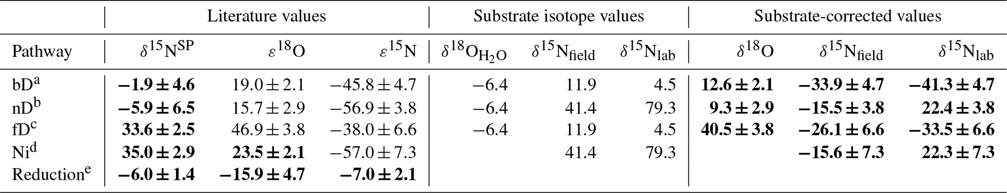
^a Barford et al. (1999); Lewicka-Szczebak et al. (2016, 2014); Rohe et al. (2017); Sutka et al. (2006); Toyoda et al. (2005). ^b Frame and Casciotti (2010); Sutka et al. (2006). ^c Maeda et al. (2015); Rohe et al. (2014a, 2017); Sutka et al. (2008). ^d Frame and Casciotti (2010); Mandernack et al. (2009); Sutka et al. (2006); Yoshida (1988). ^e Jinuntuya-Nortman et al. (2008); Lewicka-Szczebak et al. (2015, 2014); Menyailo and Hungate (2006); Ostrom et al. (2007); Well and Flessa (2009).

Download Print Version | Download XLSX

2.6 Three-dimensional N₂O isotopocule model (3DIM)

The probability distributions of proportional contributions f_i were determined using a stable isotope mixing model in the Bayesian framework. This allowed us to integrate three N₂O isotopic signatures into one model to find the nearest solution for the $r_{{\mathrm{N}}_{\mathrm{2}}\mathrm{O}}$ and mixing proportions. The core of the model was based on the work of Moore and Semmens (2008), which was further extended with implementation of N₂O reduction in two possible cases (analogically as for MAPs – see Sect. 2.5).

where f stands for fraction of N₂O originating from a particular pathway and δ stands for isotopic signature characteristic of this pathway for bD, nD, fD, and nitrification Ni; ε is the isotope fractionation factor for N₂O reduction to N₂, and $r_{{\mathrm{N}}_{\mathrm{2}}\mathrm{O}}$ is the N₂O residual fraction as defined in Eq. (10); r_bD is the N₂O residual fraction of bacterial denitrification only, as it is assumed in Case 1. This value can be recalculated to obtain $r_{{\mathrm{N}}_{\mathrm{2}}\mathrm{O}}$ as follows:

Let us briefly summarize the key assumptions and features of the statistical model. The input data of measured m isotope signatures (here three: δ¹⁵N, δ¹⁵N^SP, δ¹⁸O) from n sources (here four: bD, nD, fD, and Ni) are assumed to be normally distributed, and multiple measurements (here one to seven replicates) constitute a single sample, on which the Monte Carlo integration is performed. The uncertainties in the source data are fed into the model through the variance in the calculation of unnormalized likelihood (see Eq. 18). For prior distributions of parameters, a flat Dirichlet distribution was used for proportional source contributions f_i and uniform distribution for reduction parameter r. For each random sample (f_i,r), a mean and a variance of each isotope signature j are calculated (different for two cases listed above):

and the likelihood of such a combination is calculated as

where x_kj stands for kth measurement of the sample and jth isotope signature. We use the Markov-chain Monte Carlo method with the Metropolis condition: $L_{i+\mathrm{1}}/L_i\ge \mathit{\alpha }$, where α is a random variable sampled from a uniform distribution.

The detailed input parameters for the model are presented in Table 1. The detailed isotopic characteristics to be applied for the isotope signatures of mixing endmembers and reduction fractionation factors are adopted after the most recent review paper (Yu et al., 2020).

2.7 Statistics

For results comparisons, an analysis of variance was used with the significance level α of 0.1. The uncertainty values provided for the measured parameters represent the standard deviation (1σ) of the replicates. The propagated uncertainty was calculated using the Gauss error propagation equation, taking into account standard deviations of all individual parameters.

The agreement with the reference method was assessed with the Nash–Sutcliffe efficiency (F) (Nash and Sutcliffe, 1970), which represents the R of the fit to the 1:1 line between observed reference (O) and estimated (E) values, as also used in previous validation studies (Lewicka-Szczebak et al., 2017; Wu et al., 2019):

where E_i is the $r_{{\mathrm{N}}_{\mathrm{2}}\mathrm{O}}$ value estimated with the method under validation, corresponding to the observed $r_{{\mathrm{N}}_{\mathrm{2}}\mathrm{O}}$ value determined with the reference method (O_i), and O is the observed mean. In this assessment, an F=1 refers to a perfect fit between estimated and reference values, lower F values indicate worse model fits, and a negative F occurs when the observed mean is a better predictor than the model.

3.1 Soil properties

Soil organic N was analyzed in soil samples from each sampling campaign and varied only slightly with content of 0.141 %±0.007 % N and isotopic signature δ¹⁵N of 7.4 ‰±0.4 ‰. δ¹⁸O of soil water varied only slightly for field campaigns and equaled −6.7 ‰ for F1, −7.0 ‰ for F2, and −6.4 ‰ for F3, but was higher for incubation experiments with mean of −5.3 ‰. Detailed characteristics for mineral nitrogen contents and isotopic signatures are presented in Table 2. The variations in water and nitrate content during the field campaigns and laboratory incubations with comparison between NA and ¹⁵N treatment are presented in the Supplement (Fig. S1). Importantly, for the vast majority of sampling points these soil conditions are well comparable between both treatments, which allows for the comparison of the methods. Significant difference was only noted for nitrate content for the last sample in L2 and for water content for the last sample in F1 (Fig. S1).

3.2 Field campaigns

The first field campaign (F1) in November 2015 (23–27 November) showed low N₂O fluxes from 1.2 to 33.2 g N-N₂O ${\mathrm{ha}}^{-\mathrm{1}}{\mathrm{d}}^{-\mathrm{1}}$ (Table 2). N₂O isotopic signatures were determined for all the samples except one. The N₂ fluxes were under the detection limit for all samples, i.e., below 11 g N-N₂ ${\mathrm{ha}}^{-\mathrm{1}}{\mathrm{d}}^{-\mathrm{1}}$. In this case, the reference $r_{{\mathrm{N}}_{\mathrm{2}}\mathrm{O}}$ values from the ¹⁵N treatment could not be precisely determined. However, from the information that N₂ flux is below the detection limit even for the highest N₂O fluxes observed, we can assess that $r_{{\mathrm{N}}_{\mathrm{2}}\mathrm{O}}$ must be higher than 0.75. For F1, soil temperature varied from 1.6 to 8.6 ^∘C (mean 4.1 ^∘C); WFPS varied from 54.1 to 72.4 % (mean 65 %).

The second field campaign (F2) in March 2016 (7–11 March) showed very variable N₂O fluxes from 0.5 to 110.7 g N-N₂O ${\mathrm{ha}}^{-\mathrm{1}}{\mathrm{d}}^{-\mathrm{1}}$. N₂O isotopic signatures could be determined only in 17 samples from 26. The N₂ fluxes were above the detection limit for 15 samples from 26, and they varied from 23 to 304 g N-N₂ ${\mathrm{ha}}^{-\mathrm{1}}{\mathrm{d}}^{-\mathrm{1}}$. In this case, the reference $r_{{\mathrm{N}}_{\mathrm{2}}\mathrm{O}}$ values from the ¹⁵N treatment could be determined for four sampling dates out of eight. For F2, soil temperature varied from 1.4 to 12.0 ^∘C (mean 6.4 ^∘C); WFPS varied from 57.9 to 77.9 % (mean 69 %).

The third field campaign (F3) in May/June 2016 (30 May–3 June) showed very high N₂O fluxes from 1 to 1471 g N-N₂O ${\mathrm{ha}}^{-\mathrm{1}}{\mathrm{d}}^{-\mathrm{1}}$. N₂O isotopic signatures could be determined in all samples. The N₂ fluxes were always above the detection limit and varied from 114 to 2060 g N-N₂ ${\mathrm{ha}}^{-\mathrm{1}}{\mathrm{d}}^{-\mathrm{1}}$. In this case, the reference $r_{{\mathrm{N}}_{\mathrm{2}}\mathrm{O}}$ values from the ¹⁵N treatment could be determined for all eight sampling times. For F3, soil temperature varied from 17.0 to 32.5 ^∘C (mean 21.4 ^∘C); WFPS varied from 52.1 % to 72.0 % (mean 62 %).

The detailed variations in gas fluxes during field campaigns, variations in ¹⁵N abundance in various pools ($a_{{\mathrm{NO}}_{\mathrm{3}}}$, $a_{\text{P\_}{\mathrm{N}}_{\mathrm{2}}\mathrm{O}}$, and $a_{\text{P\_}{\mathrm{N}}_{\mathrm{2}}}$), and the N₂O ¹⁵N-pool-derived fraction ($f_{\text{P\_}{\mathrm{N}}_{\mathrm{2}}\mathrm{O}}$) are presented in the Supplement (Figs. S2c–e and S3c–e). There are no significant differences in N₂O flux between ¹⁵N and NA treatment (Fig. S2c–e). In F3 the fluxes were much larger than in F1 and F2 and were decreasing during the sampling campaign, whereas N₂ flux was very variable and showed large differences between repetitions, represented by large error bars (Fig. S2e). In F1 and F2, the ¹⁵N-pool-derived fraction was significantly lower when compared to F3. In F3, $a_{\text{P\_}{\mathrm{N}}_{\mathrm{2}}}$ and $a_{\text{P\_}{\mathrm{N}}_{\mathrm{2}}\mathrm{O}}$ were comparable and higher than $a_{{\mathrm{NO}}_{\mathrm{3}}}$ in the first three samples and similar with $a_{{\mathrm{NO}}_{\mathrm{3}}}$ for the last five samples. In F2, $a_{\text{P\_}{\mathrm{N}}_{\mathrm{2}}\mathrm{O}}$ strictly depended on $a_{{\mathrm{NO}}_{\mathrm{3}}}$, and both showed clear decreasing trends, whereas $a_{\text{P\_}{\mathrm{N}}_{\mathrm{2}}}$ was determined only in two sampling points and was significantly lower than $a_{\text{P\_}{\mathrm{N}}_{\mathrm{2}}\mathrm{O}}$ and $a_{{\mathrm{NO}}_{\mathrm{3}}}$.

3.3 Laboratory experiments

The laboratory experiment L1 was conducted in dryer conditions than L2. In L1 initially WFPS was about 60 %, and after water addition (9th day of the experiment) it was increased to 65 %. In L2 initially WFPS was about 70 %, and after water addition (9th day of the experiment) it was increased to 80 %. N₂O fluxes in L1 were quite low: from 0.2 to 16.7 g N-N₂O ${\mathrm{ha}}^{-\mathrm{1}}{\mathrm{d}}^{-\mathrm{1}}$. N₂O isotopic signatures could be determined in 38 out of 56 samples. The N₂ fluxes were above the detection limit only for 43 out of 112 samples and varied from 1.5 to 69.4 g N-N₂ ${\mathrm{ha}}^{-\mathrm{1}}{\mathrm{d}}^{-\mathrm{1}}$. In this case the reference $r_{{\mathrm{N}}_{\mathrm{2}}\mathrm{O}}$ values from the ¹⁵N treatment could only be determined for 7 sampling times out of 10. In L2 N₂O fluxes were higher and varied in a wide range from 0.4 to 297.4 g N-N₂O ${\mathrm{ha}}^{-\mathrm{1}}{\mathrm{d}}^{-\mathrm{1}}$. N₂O isotopic signatures could be determined in 40 out of 56 samples. The N₂ fluxes were above the detection limit only for 87 out of 112 samples and varied from 1.2 to 199 g N-N₂ ${\mathrm{ha}}^{-\mathrm{1}}{\mathrm{d}}^{-\mathrm{1}}$. In this case, the reference $r_{{\mathrm{N}}_{\mathrm{2}}\mathrm{O}}$ values from the ¹⁵N treatment could be determined for 9 sampling times out of 10.

Table 2Results summary.

^a determined in ¹⁵N treatments with gas-flux method
^b half of data below detection limit
bd – below detection limit
nd – not determined, due to N₂ flux below detection limit

Download Print Version | Download XLSX

The detailed variations in gas fluxes during laboratory incubations, variations in ¹⁵N abundance in various pools ($a_{{\mathrm{NO}}_{\mathrm{3}}}$, $a_{\text{P\_}{\mathrm{N}}_{\mathrm{2}}\mathrm{O}}$, and $a_{\text{P\_}{\mathrm{N}}_{\mathrm{2}}}$), and the N₂O ¹⁵N-pool-derived fraction ($f_{\text{P\_}{\mathrm{N}}_{\mathrm{2}}\mathrm{O}}$) are presented in the Supplement (Figs. S2a, b and S3a, b). We often observe significantly different fluxes for NA and ¹⁵N treatment: for L1 only for two samples (4 and 5) NA treatment showed significantly higher N₂O flux, but for L2 the majority of sampling points shows a significantly higher N₂O flux in the ¹⁵N treatment, particularly for the last four sampling points, after the water addition (Fig. S2b). Importantly, water content did not differ for these sampling points. In L1 the ¹⁵N-pool-derived fraction was significantly lower when compared to L2. In both L1 and L2, $a_{\text{P\_}{\mathrm{N}}_{\mathrm{2}}}$, $a_{\text{P\_}{\mathrm{N}}_{\mathrm{2}}\mathrm{O}}$, and $a_{{\mathrm{NO}}_{\mathrm{3}}}$ showed comparable ranges and only a very slight decreasing trend (Fig. S3a, b).

3.4 MAPs

O ∕ SP MAP

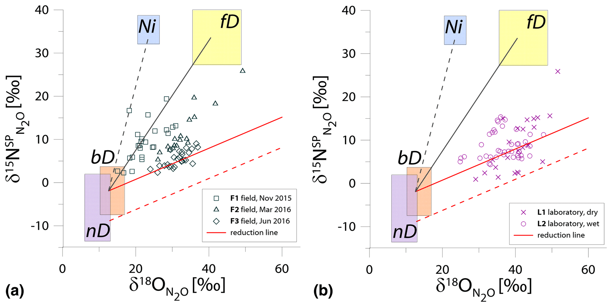
Figure 1N₂O isotope data of field (a, green points) and laboratory studies (b, purple points) in SP∕O MAP presented with literature endmember values and theoretical mixing (grey line) and reduction (red line) lines. The solid lines (bD-fD mixing and mean reduction line) are main assumptions used in the calculation procedures for SP∕O MAP. The dashed grey line shows the alternative bD-Ni mixing line (calculations with this alternative scenario are also presented in Table S1 in the Supplement). The dashed red line shows the minimum reduction line – for the case of minimal delta values of the bD endmember. δ¹⁸O values of mixing endmember bD, nD, and fD are presented in relation to the mean measured ambient water of −6.4 ‰ (hence present the expected δ¹⁸O${}_{{\mathrm{N}}_{\mathrm{2}}\mathrm{O}}$ originating from a particular pathway in these study conditions).

Download

The majority of isotope results presented in the SP∕O MAP (Fig. 1) is situated within the area limited by reduction and mixing lines, which allows for application of the calculation approach based on SP∕O MAP. Numerous samples, mostly from the laboratory incubation studies, are situated below the mean reduction line but within the minimum reduction line. For these samples, the calculation results provide f_bD values slightly above 1, which are set to 1 for the further summaries. All calculations and results can be followed in the spreadsheet file in the Supplement.

The endmember isotope values applied here (after Yu et al., 2020) differ for nitrification δ¹⁸O when compared to previous applications of SP∕O MAP (Buchen et al., 2018; Ibraim et al., 2019; Lewicka-Szczebak et al., 2017; Verhoeven et al., 2019). The currently applied δ¹⁸O endmember values for Ni (23.5 ‰±2.1 ‰) are lower than the previously applied range (from 38.0 ‰ to 55.2 ‰, mean 43.0 ‰) and thus result in a separation of Ni and fD, which was not possible in the previous studies. With the current values, we have two possible mixing lines (bD-Ni and bD-fD), whereas in previous studies only one mixing line was applied (bD − (Ni + fD)). This requires the choice of the most appropriate mixing scenario for the particular case study. For this study, the results obtained for $r_{{\mathrm{N}}_{\mathrm{2}}\mathrm{O}}$ and f_bD differ (mostly) only very slightly for both mixing scenarios (see Table S1 and spreadsheet file in the Supplement), which is due to high f_bD. For F3, where f_bD is near 1, the difference in $r_{{\mathrm{N}}_{\mathrm{2}}\mathrm{O}}$ does not exceed 0.02, and for F1 with the lowest f_bD of ca. 0.7, the difference in $r_{{\mathrm{N}}_{\mathrm{2}}\mathrm{O}}$ reaches 0.22 (Table S1). Below we summarize the results of calculations assuming the bD-fD mixing scenario only.

The calculation has been performed with two cases (see Sect. 2.5), and all results are shown and compared with reference method in Tables 3 and 4. Due to quite high f_bD for our study, both cases show only very slight differences (Tables 3 and 4). For the field study F1, we obtained the highest $r_{{\mathrm{N}}_{\mathrm{2}}\mathrm{O}}$ values (0.86±0.12) and the lowest f_bD values (0.74±0.07). For field study F2, the $r_{{\mathrm{N}}_{\mathrm{2}}\mathrm{O}}$ values were lower (0.38±0.05) and the f_bD values were higher (0.92±0.04). For field study F3, the $r_{{\mathrm{N}}_{\mathrm{2}}\mathrm{O}}$ values were very similar as in F2 (0.33±0.07) and the highest f_bD values were noted (0.99±0.01). For the laboratory incubation studies, we obtained slightly lower (p=0.086) $r_{{\mathrm{N}}_{\mathrm{2}}\mathrm{O}}$ for L1 (0.19±0.03) when compared to L2 (0.27±0.12). Both laboratory treatments showed very high f_bD for L1 (0.99±0.01) and L2 (0.98±0.04).

N ∕ SP MAP

Figure 2N₂O isotope data of field (green points) and laboratory (purple points) in SP∕N MAP presented with literature mixing endmember values and theoretical mixing (grey line) and reduction (red line) lines. δ¹⁵N values of mixing endmembers are presented in relation to the δ¹⁵N of precursors: soil nitrate for bD and fD or ammonium for nD and Ni (hence present the expected δ¹⁵N${}_{{\mathrm{N}}_{\mathrm{2}}\mathrm{O}}$ originating from a particular pathway in these study conditions).

Download

For the SP∕N MAP, we present the literature endmember values in relation to the respective precursor, i.e., ${\mathrm{NO}}_{\mathrm{3}}^{-}$ for bD and fD and ${\mathrm{NH}}_{\mathrm{4}}^{+}$ for nD and Ni (Table 1). For the field and laboratory studies, separate mean values for ${\mathrm{NO}}_{\mathrm{3}}^{-}$ (11.9 ‰ and 4.5 ‰, respectively) and ${\mathrm{NH}}_{\mathrm{4}}^{+}$ (41.4 ‰ and 79.3 ‰, respectively) were applied. These precursor isotopic signatures are the means of five samplings for each campaign and experiment. The extremely ¹⁵N-enriched δ¹⁵N${}_{{\mathrm{NH}}_{\mathrm{4}}}$ values result in a large shift of endmember ranges for nD and Ni. These ranges are ¹⁵N-depleted in relation to bD when assuming identical δ¹⁵N values for ${\mathrm{NO}}_{\mathrm{3}}^{-}$ and ${\mathrm{NH}}_{\mathrm{4}}^{+}$, according to most previous studies (Ibraim et al., 2019; Koba et al., 2009; Toyoda et al., 2011). But in the case of our experiments, conversely, N₂O originating from nD and Ni would be significantly enriched in ¹⁵N when compared to bD and fD (Fig. 2). For the samples, the measured bulk δ¹⁵N${}_{{\mathrm{N}}_{\mathrm{2}}\mathrm{O}}$ is plotted.

The majority of the samples is located outside the area limited by reduction and bD-fD mixing lines, which mostly precludes the application of the calculation approach based on SP∕N MAP. The separation of mixing and reduction processes is not possible based on this plot, since the slopes of reduction line and bD-Ni mixing line are too similar, especially for laboratory experiments (Fig. 2b).

Another approach to include N precursor values is to apply the individual endmember isotopic signatures for each N₂O sample by interpolating the measured isotopic signatures of ${\mathrm{NO}}_{\mathrm{3}}^{-}$ and ${\mathrm{NH}}_{\mathrm{4}}^{+}$. With five measurements of mineral N isotopic signatures per experiment, we get quite a good resolution for these values. Since they show quite high variations (Table 2), applying individual values is a better approach. But still (also by this approach), the majority of samples show values out of the calculation range, and the results are very ambiguous, representing the whole range of possible variations in both $r_{{\mathrm{N}}_{\mathrm{2}}\mathrm{O}}$ and f_bD values. Therefore these values are not summarized here.

O ∕ N MAP

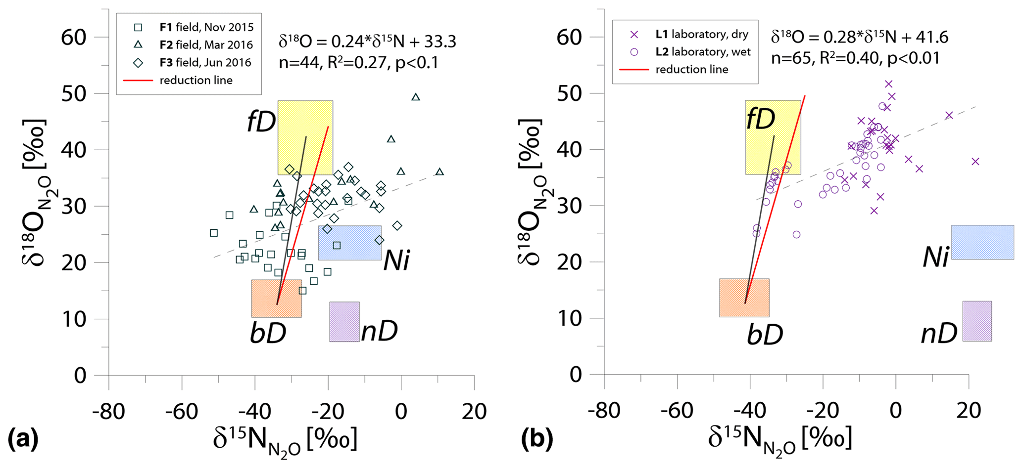
Figure 3N₂O isotope data of field (a, green points) and laboratory (b, purple points) in O∕N MAP presented with literature mixing endmember values and theoretical mixing (grey line) and reduction (red line) lines. δ¹⁵N values are presented in relation to the δ¹⁵N of precursors: soil nitrate for bD and fD or ammonium for nD and Ni. δ¹⁸O values of mixing endmember bD, nD, and fD are presented in relation to the mean measured ambient water of −6.4 ‰. Hence, the mixing endmember ranges present the expected δ¹⁵N${}_{{\mathrm{N}}_{\mathrm{2}}\mathrm{O}}$ and δ¹⁸O${}_{{\mathrm{N}}_{\mathrm{2}}\mathrm{O}}$ originating from a particular pathway in these study conditions. The dashed line shows the linear fit for all the points with its equation and statistics above.

Download

For O∕N MAP (Fig. 3), the δ¹⁸O values for bD, fD, and nD are expressed in relation to soil water; the δ¹⁵N values for bD and fD are expressed in relation to soil ${\mathrm{NO}}_{\mathrm{3}}^{-}$ and for nD and Ni in relation to soil ${\mathrm{NH}}_{\mathrm{4}}^{+}$ (Table 1). For these graphs, it is difficult to determine the reduction-mixing area because the slope of the reduction line is almost identical to the bD-fD mixing line.

A significant linear correlation has been found for both the field and laboratory studies, with R²=0.27 (p<0.1) and R²=0.40 (p<0.01), respectively. Both correlations show similar linear equations: ${\mathit{\delta }}^{\mathrm{18}}\mathrm{O}=\mathrm{0.24}\times {\mathit{\delta }}^{\mathrm{15}}\mathrm{N}+\mathrm{33.3}$ and ${\mathit{\delta }}^{\mathrm{18}}\mathrm{O}=\mathrm{0.28}\times {\mathit{\delta }}^{\mathrm{15}}\mathrm{N}+\mathrm{41.6}$ for field and laboratory studies, respectively (Fig. 3).

3.5 3DIM

The application of MAPs applying δ¹⁵N data, i.e., SP∕N MAP and O∕N MAP, is very imprecise for this case study due to untypically high δ¹⁵N${}_{{\mathrm{NH}}_{\mathrm{4}}}$ values and shifted location of the nD and Ni mixing endmembers (Figs. 2 and 3) when compared to cases when similar δ¹⁵N${}_{{\mathrm{NH}}_{\mathrm{4}}}$ and δ¹⁵N${}_{{\mathrm{NO}}_{\mathrm{3}}}$ values are determined or assumed. However, still the δ¹⁵N data comprise important information, which can assist in process identification when applied jointly with the SP∕O MAP. Therefore, we combined all the information into one 3DIM where all three isotopic signatures are taken into account.

The results of this model regarding $r_{{\mathrm{N}}_{\mathrm{2}}\mathrm{O}}$ are mostly well comparable to the values obtained with SP∕O MAP (Table 3). However, for SP∕O MAP both Case 1 and Case 2 provide similar results for $r_{{\mathrm{N}}_{\mathrm{2}}\mathrm{O}}$, whereas for 3DIM these differ more pronouncedly. With the bar plots (Fig. 4) we summarize the results obtained from both modeling cases and below we summarize the results of Case 2, which provides more reliable results, as further discussed (see Sect. 4.2).

We get a much more detailed estimation regarding mixing proportions with 3DIM when compared to the SP∕O MAP. The dominating N₂O production pathway is clearly bD, which contributes to N₂O production from 46 % for F2 up to 69 % for L2 (Fig. 4). An important role is also played by nD by contributing from 15% for L2 up to 40% N₂O for F3; low f_nD of 4 % was found for F1. The f_fD is quite variable from 6 % for F3 to 26 % for F1. Ni shows the lowest contribution around 3 %–5 %, and only a slightly higher f_Ni of 13 % was found for F2 (Fig. 4). N₂ fluxes are highly variable between the experiments, i.e., mean $r_{{\mathrm{N}}_{\mathrm{2}}\mathrm{O}}$ values vary from 0.21 for L1 to 0.89 for F1 (Fig. 4, Table 3).

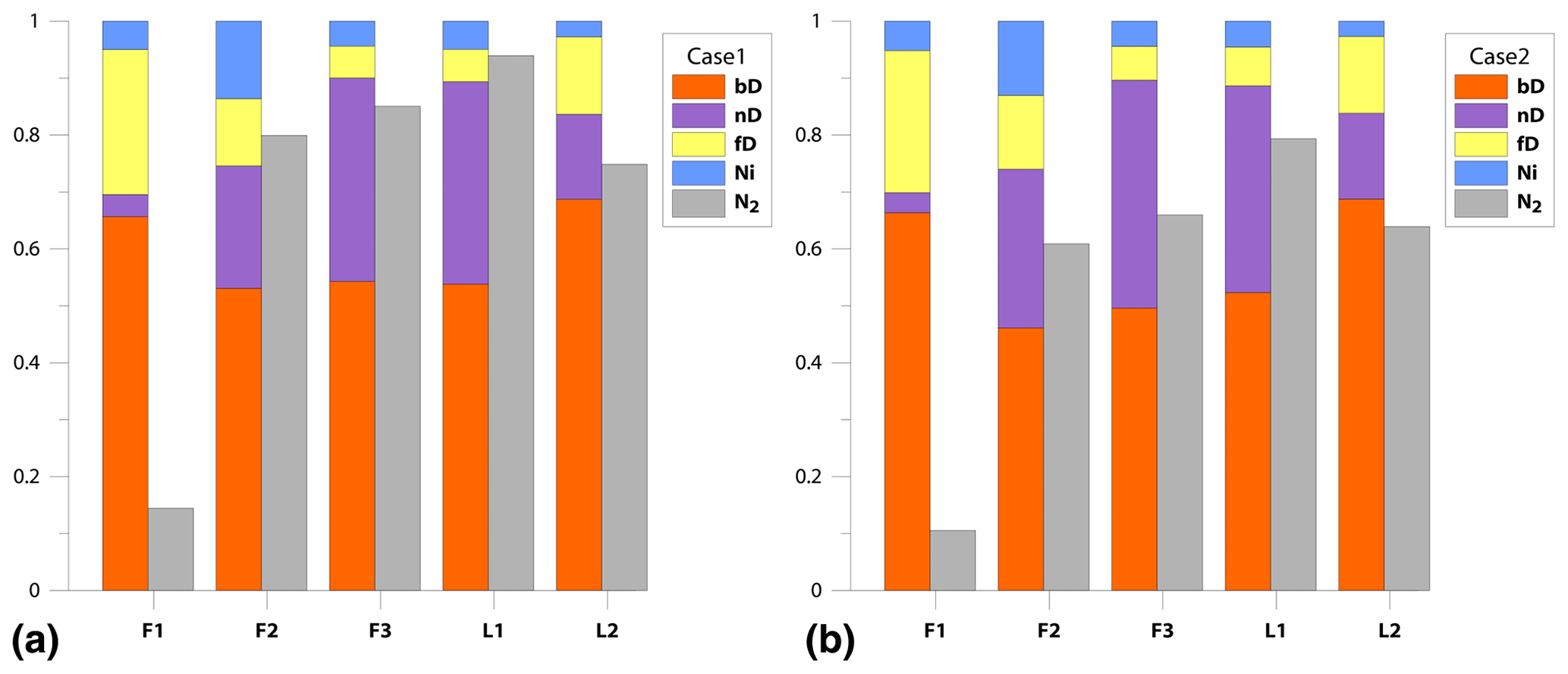
Figure 4Bar plots showing modeled pathway fractions (f_bD, f_nD, f_fD, f_Ni) and N₂ flux contribution in the total (N₂+N₂O) flux ($\mathrm{1}-r_{{\mathrm{N}}_{\mathrm{2}}\mathrm{O},}$). Results for both modeling cases, Case 1 (a) and Case 2 (b), are shown.

Download

The model provides very detailed information on probability distribution of the results, which is presented on the matrix plots prepared after Parnell et al. (2013) (Fig. S4 in the Supplement), where histograms of probability distribution of $r_{{\mathrm{N}}_{\mathrm{2}}\mathrm{O}}$ and mixing proportions, correlations between the modeled fractions, and R coefficients of these correlations are presented (Fig. S4). This summary provides an overview of the reliability of the model outputs and allows for identifying unavoidable model inadequacy. For all the modeled random samples, we observe very strong negative correlation between f_bD and f_nD, similar for both cases, from −0.28 to −0.93 (mean −0.63) and between f_bD and f_fD from −0.15 to −0.97 (mean −0.74); $r_{{\mathrm{N}}_{\mathrm{2}}\mathrm{O}}$ for Case 2 is always correlated negatively with f_bD from −0.15 to −0.84 (mean −0.62) and positively with f_fD from 0.18 to 0.82 (mean 0.62). For Case 1, this correlation is extremely variable for $r_{{\mathrm{N}}_{\mathrm{2}}\mathrm{O}}/f_{\text{bD}}$ from −0.67 to 0.85 and for $r_{{\mathrm{N}}_{\mathrm{2}}\mathrm{O}}/f_{\text{fD}}$ from −0.72 to 0.69. The lowest correlation coefficients are noted for f_Ni, where mean values never exceed 0.4. This is reflected in the determined ranges of possible results presented in the histograms. The f_Ni range is typically much narrower than f_bD and f_nD ranges.

The correlations and histograms vary between the particular campaigns with some typical features. For F1, we observe a very similar output for Case 1 and Case 2, quite narrow ranges of results, and no extremely high correlations. For F2, the ranges are much larger and high negative correlations for f_bD∕f_nD and f_fD∕f_Ni indicate possible imprecision in separation of these pathways, which results in a much wider range of probable results. For F3, the most extreme negative correlation for f_bD∕f_nD is noted, and for Case 1 also r and f_nD show very strong correlation, which may affect the proper estimation of $r_{{\mathrm{N}}_{\mathrm{2}}\mathrm{O}}$. For L1 and L2, we observe lower correlation f_bD∕f_nD but higher f_bD∕f_fD, which is probably a result of different δ¹⁵N endmember values for nD and Ni and better separation of these pathways. The strong positive correlation of $r_{{\mathrm{N}}_{\mathrm{2}}\mathrm{O}}$ and f_bD for Case 1 in L1, F2, and F3 is rather a logical consequence of the assumptions underlying the Case 1 approach.

3.6 Comparison of $r_{{\mathrm{N}}_{\mathrm{2}}\mathrm{O}}$ with independent estimates

The N₂O reduction progress calculated with the above-presented SP∕O MAP and 3DIM were compared with the results from the ¹⁵N gas-flux method. In the tables below we present the detailed comparison with the results applying both calculation cases (Case 1 and Case 2) for $r_{{\mathrm{N}}_{\mathrm{2}}\mathrm{O}}$ (Table 3) and for mixing proportions (Table 4).

The ranges and the mean values of the replicate means of all sampling dates are well comparable for SP∕O MAP and 3DIM Case 2. Most inconsistent results are obtained in Case 1 of 3DIM; however, for L2 this case seems to be most accurate.

Since the variations of $r_{{\mathrm{N}}_{\mathrm{2}}\mathrm{O}}$ values in the experiments are very variable in time, just a comparison of overall mean values is not informative; we need to compare the temporal changes in $r_{{\mathrm{N}}_{\mathrm{2}}\mathrm{O}}$ (Fig. 5).

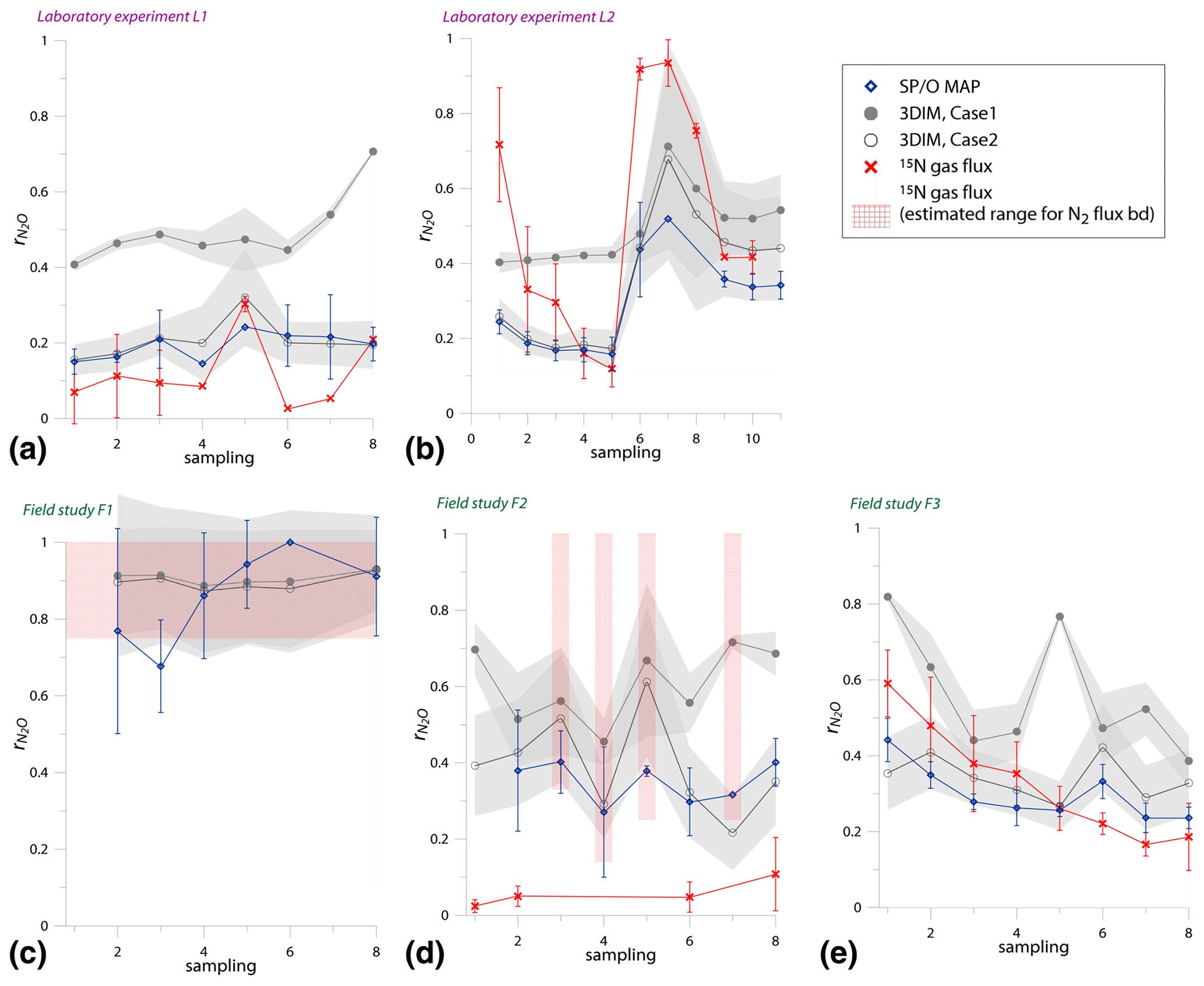
Figure 5Comparison of time changes in residual N₂O fraction ($r_{{\mathrm{N}}_{\mathrm{2}}\mathrm{O}}$) determined with O∕SP MAP Case 1 and 3DIM with the reference method (¹⁵N gas flux). For 3DIM results, the 95 % confidence interval is shown with grey shaded areas. Error bars for O∕SP MAP and ¹⁵N gas-flux data represent the standard deviation of replicate samples (n=4). For N₂ fluxes below the detection limit, the estimated $r_{{\mathrm{N}}_{\mathrm{2}}\mathrm{O}}$ values are shown (red areas), calculated with N₂ flux from 0 to 1 of the detection limit.

Download

Most extreme changes in time are reported for the laboratory experiment L2 where a very sudden change in $r_{{\mathrm{N}}_{\mathrm{2}}\mathrm{O}}$ was observed as a consequence of water addition (between sampling 5 and 6). All three estimates present the same trend as the reference method, however, with lower amplitude of the temporal change (Fig. 5b). For field study F3, ¹⁵N treatment indicates a constant decrease in $r_{{\mathrm{N}}_{\mathrm{2}}\mathrm{O}}$, which is only partially reflected in SP∕O MAP and not at all in 3DIM results. F1 and F2 data are not complete due to N₂ fluxes under detection limit for the whole F1 sampling and half of the samples of F2 campaign. However, for this missing data we can make estimates of the $r_{{\mathrm{N}}_{\mathrm{2}}\mathrm{O}}$ based on the known detection limit for N₂ flux. We estimated the $r_{{\mathrm{N}}_{\mathrm{2}}\mathrm{O}}$ values for the missing points assuming the possible N₂ flux: from 0 up to the detection limit of 11.3 g N-N₂ ${\mathrm{ha}}^{-\mathrm{1}}{\mathrm{d}}^{-\mathrm{1}}$.

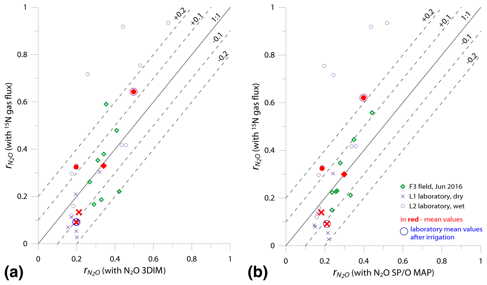
Figure 6Comparison of 1:1 fit between $r_{{\mathrm{N}}_{\mathrm{2}}\mathrm{O}}$ determined with the reference method (¹⁵N gas flux) and (a) 3DIM Case 2 and (b) SP∕O MAP Case 1.

Download

In Fig. 6 we checked the fit of $r_{{\mathrm{N}}_{\mathrm{2}}\mathrm{O}}$ values determined by ¹⁵N gas-flux method and 3DIM (Fig. 6a) or SP∕O MAP (Fig. 6b). When analyzing all the individual sampling dates or all experiments, the fit to the 1:1 line is not very good, especially for many dates of the L2 experiment $r_{{\mathrm{N}}_{\mathrm{2}}\mathrm{O}}$ is largely underestimated with isotopocule approaches. This is mostly due to the sudden change in $r_{{\mathrm{N}}_{\mathrm{2}}\mathrm{O}}$ as presented above (Fig. 5b). But when we compare the means of the whole experiment or the experimental phases before and after water addition for L1 and L2 (red points in Fig. 6), the fit is much better with all points within the error of 0.15 for 3DIM. For SP∕O MAP, the L2 mean after irrigation still shows larger disagreement.

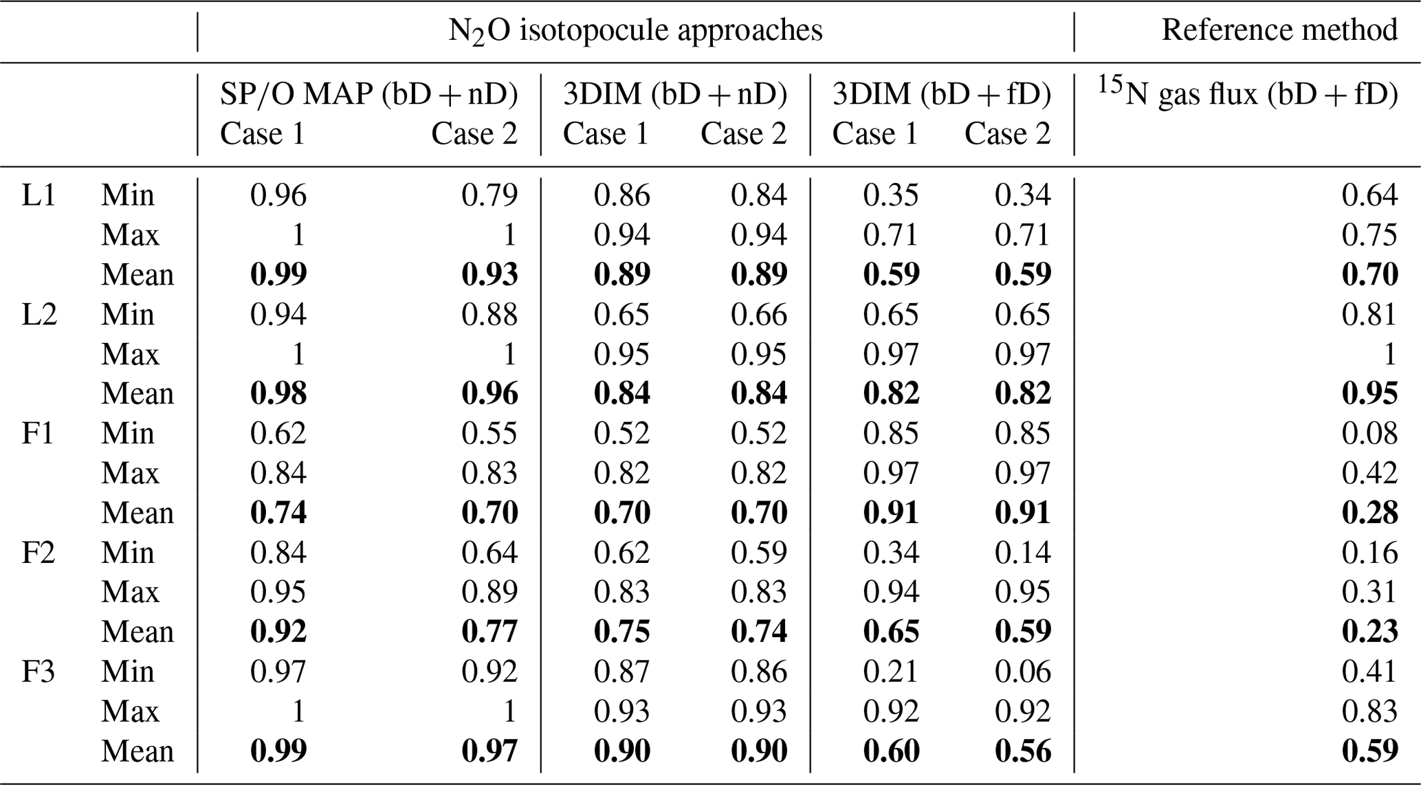
The agreement between isotopocule methods and the reference method was statistically checked with F value (Eq. 19). The results for all means, minima, and maxima are shown in Table 3. The statistically significant agreement was indicated for SP∕O MAP (p<0.1) and Case 2 of 3DIM (p<0.05), whereas Case 1 of 3DIM shows no agreement. Particular F values calculated with all sampling date means indicate no significant agreement (F=0.13 for F3, F=0.45 for L1, F=0.28 for L2 – values for fit between Case 2 of 3DIM and reference method), which reinforces the observation, based on Fig. 6, that only mean experimental values show good agreement with the reference method but not the individual samplings.

Table 3Comparison of N₂O residual fraction ($r_{{\mathrm{N}}_{\mathrm{2}}\mathrm{O}}$) determined with the N₂O isotopocule approaches (SP∕O MAP and 3DIM) and the reference method (¹⁵N gas flux). Minimal (min), maximal (max), and mean values were calculated with the each sampling mean values (of all replicates). The agreement with the reference method was assessed with the Nash–Sutcliffe efficiency (F, Eq. 19) (Nash and Sutcliffe, 1970), which represents the R² of the fit to the 1:1 line (Fig. 6).

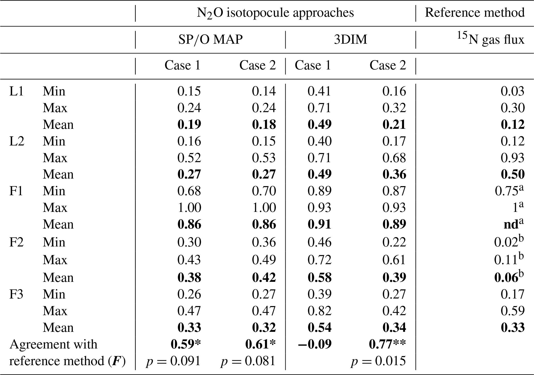
^a all N₂ fluxes under detection limit, the range of values estimated based on detection limit – values not included in the statistics
^b data not complete due to half of N₂ fluxes under detection limit – values not included in the statistics

Download Print Version | Download XLSX

3.7 Comparison of mixing proportions with independent estimates

The mixing proportions obtained by different approaches are much more complex to compare than $r_{{\mathrm{N}}_{\mathrm{2}}\mathrm{O}}$ due to the fact that each approach provides distinct information.

• With the reference method – ¹⁵N gas flux – we determine the ¹⁵N-pool-derived fraction of N₂O ($f_{\text{P\_}{\mathrm{N}}_{\mathrm{2}}\mathrm{O}}$); hence, for the ¹⁵NO${}_{\mathrm{3}}^{}$ treatment this is the fraction of N₂O originating from the labeled ¹⁵NO${}_{\mathrm{3}}^{}$ pool. Theoretically, this can be bD or fD. It was intended to use the ¹⁵NH${}_{\mathrm{4}}^{+}$ treatment for the determination of N₂O fraction derived from ${\mathrm{NH}}_{\mathrm{4}}^{+}$ pool, but due to rapid ${\mathrm{NH}}_{\mathrm{4}}^{+}$ turnover into ${\mathrm{NO}}_{\mathrm{3}}^{-}$, we deal with a highly ¹⁵N-labeled ${\mathrm{NO}}_{\mathrm{3}}^{-}$ pool in the ¹⁵NH${}_{\mathrm{4}}^{+}$ treatment and hence are not able to precisely separate these pools (results not shown).

• With SP∕O MAP, we determine thef_bD fraction. But since in the SP∕O MAP bD and nD cannot be distinguished due to overlapping isotopic signatures (Fig. 1), this fraction actually informs about the bD + nD fraction.

• With 3DIM, we are able to theoretically determine most of the fractions contributing to the N₂O flux, but the precision of such a determination depends on the isotopic separation of particular pathways in the 3D isotopocule plot. In our case study this separation is not very good, especially for δ¹⁵N (see Sect. 3.4); hence, this determination is associated with pronounced uncertainty (Fig. S4).

To compare all these results, we present a comparison of $f_{\text{P\_}{\mathrm{N}}_{\mathrm{2}}\mathrm{O}}$ of the ¹⁵N gas-flux method (representing bD + fD) with f_bD of SP∕O MAP (representing bD + nD) and respective results (f_bD, f_bD+fD, f_bD+nD) of 3DIM (Fig. 7, Table 4).

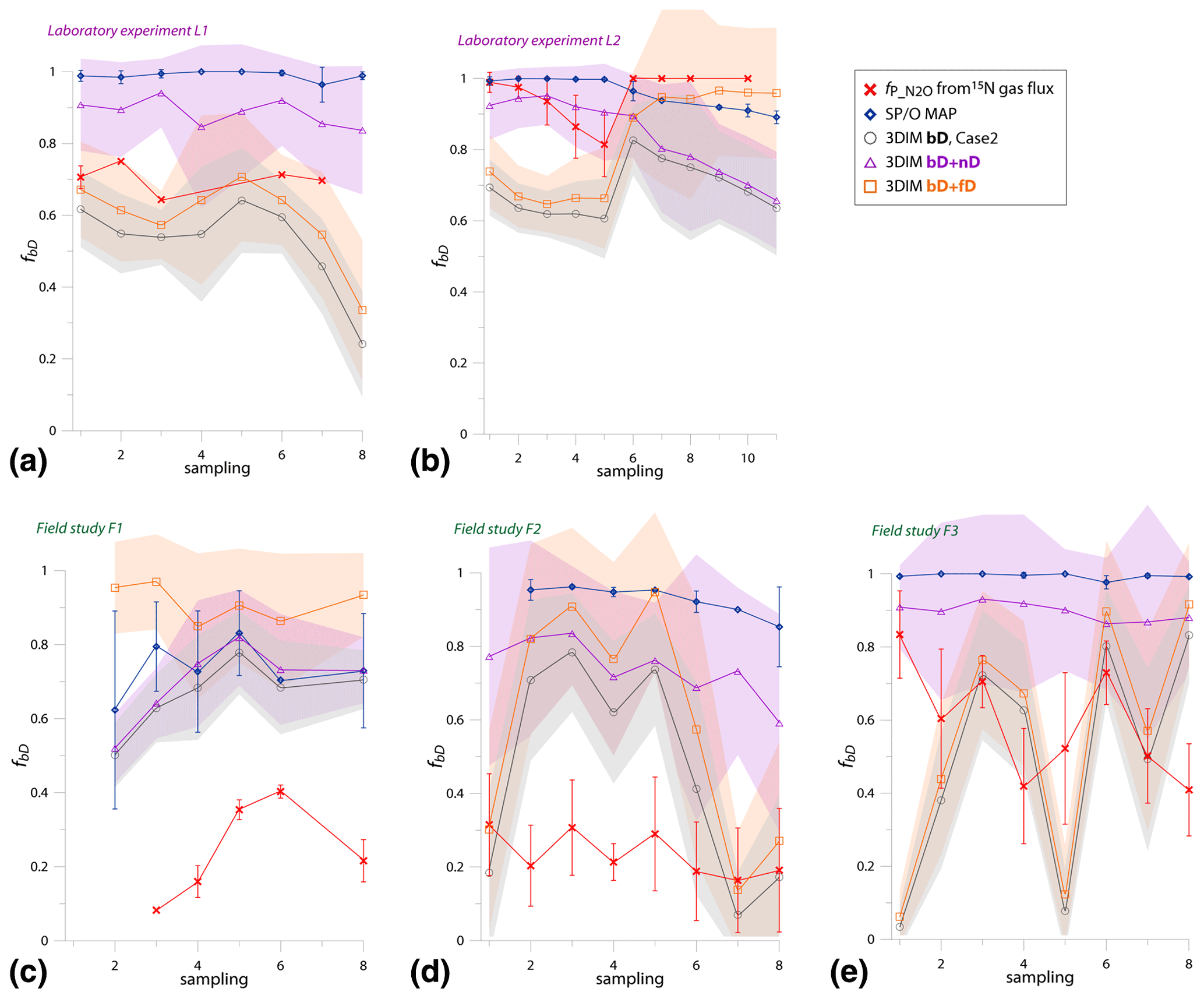
Figure 7Comparison of N₂O fractions comprising bacterial denitrification (f_bD) determined with O∕SP MAP Case 1 (representing bD + nD) and 3DIM Case 2 (respective fractions determined: bD, bD + nD, bD + fD) with the reference method (¹⁵N gas flux). The ¹⁵N gas-flux method determines the $f_{\text{P\_}{\mathrm{N}}_{\mathrm{2}}\mathrm{O}}$ – ¹⁵N-pool-derived fraction – comprising all N₂O origins utilizing ¹⁵N-labeled ${\mathrm{NO}}_{\mathrm{3}}^{-}$ – theoretically mostly bD and fD. See Sect. 4.2 and 4.3 for further discussion. For 3DIM results, the 95 % confidence interval is shown with shaded areas. Error bars for O∕SP MAP and ¹⁵N gas-flux data represent the standard deviation of replicate samples (n=4).

Download

A reasonable agreement in the ranges of values is obtained for experiments L1, L2, and F3, but a large disagreement with the reference ¹⁵N gas-flux method is observed for field studies F1 and F2 (Table 4). For these studies, extremely low $f_{\text{P\_}{\mathrm{N}}_{\mathrm{2}}\mathrm{O}}$ was found by the ¹⁵N gas-flux method of 0.28 and 0.23, respectively. The time dynamics are not very well reflected by various approaches (Fig. 7). This is mostly visible in F3 (Fig. 7e) where the f_bD and f_bD+fD show large variations between samplings from below 0.1 to above 0.9. These rapid changes show much lower amplitudes according to the ¹⁵N gas-flux approach. The contribution of f_bD+nD determined by 3DIM as well as f_bD determined by the SP∕O MAP is much more stable in time, which is especially clear for F3 (Fig. 7e) but also true for other campaigns (Fig. 7).

For the mixing proportions, the statistical agreement with F value (Eq. 19) cannot be determined, because the fractions provided by various approaches do not precisely refer to the identical pathway contributions and are not directly comparable.

4.1 MAPs for N₂O data interpretation – opportunities and limitations

So far the interpretations of N₂O isotope data are most commonly done with dual-isotope plots. Whereas SP∕N and O∕N plots were applied in numerous studies before (Kato et al., 2013; Koba et al., 2009; Opdyke et al., 2009; Ostrom et al., 2007, 2010; Toyoda et al., 2011; Well et al., 2012; Yamagishi et al., 2007; Zou et al., 2014), the usage of the SP∕O plot is quite a new idea (Lewicka-Szczebak et al., 2017), but it was already used for field studies (Buchen et al., 2018; Ibraim et al., 2019; Verhoeven et al., 2019). The recent work based on archival datasets with independent estimates of N₂ flux showed some weak accordance of the results of the SP∕O MAP with independent estimates (Wu et al., 2019). However, the reasons are difficult to identify for archival data. Here we present the performance of mapping approaches validated with independent estimates based on the ¹⁵N gas-flux method, and we try to identify potential problems.

The first challenge, especially for field studies, is obtaining complete datasets. This is due to limited sensitivity of the isotopic measurements and a need for sufficient N₂O and N₂ flux. For our first field study (F1), N₂ flux was under the detection limit and the $r_{{\mathrm{N}}_{\mathrm{2}}\mathrm{O}}$ values can thus not be fully compared. For the F2 field study, we have numerous missing data due to N₂O or N₂ flux under the detection limit; hence, only a limited number of data can be compared. This may be the main reason (besides others discussed later – Sect. 4.4) for the weakest accordance of the results for F2. For this field study, only four samples showed the N₂ flux above the detection limit, and these measured N₂ fluxes associated with the low N₂O fluxes yield very low $r_{{\mathrm{N}}_{\mathrm{2}}\mathrm{O}}$ values. For samples with N₂ flux below the detection limit, the estimated $r_{{\mathrm{N}}_{\mathrm{2}}\mathrm{O}}$ ranges also possibly show much higher values (Fig. 5d). Hence, possibly by missing the measurements of low N₂ fluxes, we miss the higher $r_{{\mathrm{N}}_{\mathrm{2}}\mathrm{O}}$ values and our calculated means are not representative of the whole experiment (Table 3).

SP∕O MAP

The SP∕O MAP was proposed (Lewicka-Szczebak et al., 2017) after it was found that δ¹⁸O of the N₂O produced by bacterial and fungal denitrification is quite stable and together with SP may be useable for discrimination of these pathways (Lewicka-Szczebak et al., 2016; Rohe et al., 2014a). As O precursor for bD, fD, and nD the soil water is accepted, under the assumption of nearly complete O exchange between water and denitrification intermediates. The high extent of O exchange during denitrification has been confirmed experimentally (Kool et al., 2009; Lewicka-Szczebak et al., 2016; Rohe et al., 2014b), and it results in a quite stable range for mixing endmember values for δ¹⁸O for bacterial and fungal denitrification (Fig. 1). Importantly, due to a higher isotope fractionation effect associated with subsequent reduction steps of ${\mathrm{NO}}_{\mathrm{3}}^{-}$ to N₂O (i.e., removal of oxygen atoms, so called branching effect) during fungal denitrification, the ranges for δ¹⁸O of bacterial and fungal N₂O differ significantly (Lewicka-Szczebak et al., 2016). Fungal denitrification shows very consequent high O exchange and high fractionation during O branching (Rohe et al., 2014b, 2017), whereas bacterial denitrification is characterized, in general, by lower fractionation, but the differences in both fractionation and O exchange between particular bacterial strains are large (Rohe et al., 2017). As a result of lower O exchange shown by some bacterial strains, δ¹⁸O${}_{{\mathrm{NO}}_{\mathrm{3}}^{-}}$ is also incorporated into produced N₂O (Rohe et al., 2017). This complicates the application of the proposed SP∕O MAP. It is not clear how large the importance of such bacterial strains is in soil communities. We assume it must be low, because soil incubation studies indicated so far mostly very high exchange rates (Kool et al., 2007; Kool et al., 2009; Lewicka-Szczebak et al., 2016). These studies covered in total 16 soils. Only for two forest soils characterized by very low N₂O emission was the O exchange around 20 % (Kool et al., 2009) and otherwise over 60 %, with mean of around 90 % (Kool et al., 2009; Lewicka-Szczebak et al., 2016). Importantly, the range of δ¹⁸O values determined for bacterial denitrification does not assume complete O exchange but is determined for the soil samples of O exchange varying in the range from 63 % to 100 % (Lewicka-Szczebak et al., 2016). Hence, based on current knowledge, this can be assumed typical for most soils and experimental conditions. Also in this study, quite a good agreement of the $r_{{\mathrm{N}}_{\mathrm{2}}\mathrm{O}}$ determined by the O∕SP MAP and the reference method (see Sect. 3.6) allows us to confirm the general assumption underlying this calculation method.

Table 4Comparison of N₂O fraction originating from bD (f_bD) determined with the N₂O isotopocule approaches (SP∕O MAP and 3DIM) and the reference method (¹⁵N gas flux). Due to methodical assumptions for the particular approach, either the bD + nD fraction (for SP∕O map and 3DIM) or the bD + fD fraction (for 3DIM and the reference method) can be compared (see Sect. 3.7).

Download Print Version | Download XLSX

4.2 3DIM – perspectives of this new approach

Such a model for interpretation of N₂O isotopic data is proposed here for the first time. This model is based on the Bayesian mixing models, being a well-established and widely applied method in food-web studies to partition dietary proportions (Parnell et al., 2013; Phillips et al., 2014). But for N₂O the determination of mixing proportion of different pathways contributing to N₂O production is further complicated by N₂O reduction, which alters the final N₂O isotopic signature. This additional parameter was incorporated into the model equations (Eqs. 13, 14). Moreover, it is still not clarified if the reduction of N₂O produced during bacterial denitrification only is possible (Case 1) or also N₂O from other pathways can be further reduced by bacterial denitrifiers (Case 2); hence, both cases need to be considered. The model has a few advantages over the SP∕O MAP. First of all, it allows for including uncertainties in input data into the model and allows for assessment of the confidence intervals for the results. Moreover, theoretically 3DIM allows for separation of four N₂O production pathways, currently identified as the most relevant, within them f_fD, which is so far not distinguishable with other isotopic methods (Wrage-Mönnig et al., 2018).

For our case studies, it has been shown that δ¹⁵N values are not useful in dual-isotope plots for quantitative estimations (Figs. 2 and 3, Sect. 3.4) but are helpful to constrain mixing proportions when incorporated into 3DIM. Since the model is based on a probability distribution, it allows for providing estimates even for imprecise data, e.g., as in our case by difficulties in proper determination of δ¹⁵N endmember ranges due to very unstable precursor isotopic signatures.

The model outputs allow us to assess the quality of model performance and reliability of the results (Fig. S4, Sect. 3.5). From the uncertainty analysis provided by the model, we can determine the confidence intervals for the estimated values (Figs. 5 and 7). This is a total uncertainty resulting from all possible uncertainty sources due to ranges of endmember values and fractionation factors, variations in N₂O isotopic signatures for one sampling date, and convergence of possible model results for three isotopic signatures. We are not able to separate these uncertainties in this study.

Another measure of model performance is given by the correlations between obtained results of all the modeled probable solutions (Fig. S4). Previous studies applying similar models interpreted the strong negative correlations between determined mixing proportions as inability of the model to distinguish these sources (Moore and Semmens, 2008; Parnell et al., 2013; Phillips et al., 2014). We observe strong negative correlations between f_bD and f_nD for most cases. This may indicate the uncertainty in determination of these fractions due to the lack of isotopic separation of these processes in the δ¹⁵N^sp∕δ¹⁸O space (Fig. 1). But such a correlation is also expected if we deal with two strongly dominating sources, and the correlations between f_bD and f_nD are indeed highest for F3, where the fractions of other pathways are lowest. Nevertheless, for fractions showing high correlations, presentation of the sum of these pathways may be much more informative than separation between them. Therefore, we observe much more stable results for the sum of f_bD and f_nD than for f_bD alone (Fig. 7). However, the large variations of f_bD are not only the modeling artifact but they also reflect the variations noted with the reference method, which is especially clear for F3 (see Fig. 7e). In this case study, we can see that the variations of f_bD are larger than in the reference method, but similar dynamics of these variations can be observed.

With the model, we can quantify the contribution of four pathways; however, there are so far no precise enough reference methods to validate these results (Wrage-Mönnig et al., 2018) (see Sect. 3.7). But are the provided estimates plausible? We can check with the most characteristic outcomes. For F1, the highest f_fD values were noted (Fig. 4). For this field study, also the highest $r_{{\mathrm{N}}_{\mathrm{2}}\mathrm{O}}$ and the lowest f_bD were noted by all the approaches (Tables 3 and 4, Figs. 5c and 7c). Since for fD N₂O is mostly the final product not further reduced to N₂ (Sutka et al., 2008), the higher f_fD should result in higher $r_{{\mathrm{N}}_{\mathrm{2}}\mathrm{O}}$ values, which was noted for F1. The highest f_Ni was noted for F2. In this field study, the soil ammonium content is clearly the highest and nitrate the lowest (Table 2), which indicates that nitrification can be more active here during the whole study campaign, when compared to the other experiments, where we deal with large ammonium consumption at the very beginning of the experiments. This accordance of results allows us to suppose that the general trends in pathway mixing proportions provided by the model is plausible.

4.3 Agreement in estimates of isotopocule approaches and independent estimates

In general, the both cases of SP∕O MAP and Case 2 of 3DIM show very similar results, whereas Case 1 of 3DIM indicates always higher $r_{{\mathrm{N}}_{\mathrm{2}}\mathrm{O}}$ values and hence underestimates N₂ flux (Table 3, Fig. 5). For the SP∕O MAP, the application of different calculation cases has little impact on the final results because both cases show very high and quite stable f_bD. The contribution of bD is expressed jointly with nD for the SP∕O MAP, due to their isotopic overlap (see Sect. 3.4). As a result, the necessary assumption for the SP∕O MAP is the possible reduction of N₂O originating from both of these fractions (bD and nD, also for Case 1). Conversely for 3DIM, both these fractions are separated, and for Case 1 only the bD fraction can be reduced. The r_bD values obtained for Case 1 are very low (e.g., 0.2 for F2 and 0.15 for F3), but when recalculated to $r_{{\mathrm{N}}_{\mathrm{2}}\mathrm{O}}$ (for comparison with other results), they become high (e.g., 0.58 for F2 and 0.54 for F3, Table 3) due to respective f_bD values (see Eq. 15). Therefore, the $r_{{\mathrm{N}}_{\mathrm{2}}\mathrm{O}}$ determined by 3DIM Case 1 is very vulnerable to proper determination of f_bD. And this fraction is not very precisely determined, as we know from strong correlation found for f_bD∕f_nD (see Sect. 4.2). Consequently, the imprecise separation of f_bD andf_nD is the reason for the biased $r_{{\mathrm{N}}_{\mathrm{2}}\mathrm{O}}$ values for Case 1 3DIM. This bias is not significant when we deal with very high $r_{{\mathrm{N}}_{\mathrm{2}}\mathrm{O}}$ fraction, as for F1 (Table 3) or for very high and stable bD contribution, as for L2 (Table 3, Fig. 7b). For Case 2, the lack of precision in f_bD and f_nD determination do not largely affect $r_{{\mathrm{N}}_{\mathrm{2}}\mathrm{O}}$ results, since N₂O originating from all pathways can be reduced in this case (Eq. 14). Hence, in further discussion of the 3DIM results, we take into account Case 2 outputs only. This observation may also indicate that it is not just N₂O from heterotrophic bacterial denitrification that can be further reduced to N₂. Although previous studies suggested Case 1 to be more accurate (Verhoeven et al., 2019; Wu et al., 2019), our comparison indicates that Case 1 of 3DIM underestimates the N₂O reduction in most cases (Table 3). This may reinforce a recent discussion on nitrifier denitrification mechanisms assuming that heterotrophic bacterial denitrifiers are relevant in reducing ${\mathrm{NO}}_{\mathrm{2}}^{-}$ from nitrification (Hink et al., 2017). This would support the assumption that N₂O from nD can be further reduced by the bD pathway.

The largest discrepancy in $r_{{\mathrm{N}}_{\mathrm{2}}\mathrm{O}}$ between isotopocule approaches and the reference method is noted for F2 (Table 3). In this field campaign we deal with very low N₂O fluxes and the reference method indicates very low $r_{{\mathrm{N}}_{\mathrm{2}}\mathrm{O}}$ values, i.e., very high N₂O reduction rate. Moreover, for F2 the highest soil moisture of the field studies was noted (Table 2), which may result in inhibition of gaseous exchange. In these conditions, it is very probable that some of the produced N₂O is completely reduced; consequently, the isotopic information on its reduction is missed. Complete N₂O reduction in soil microsites would result in overestimation of $r_{{\mathrm{N}}_{\mathrm{2}}\mathrm{O}}$ values by the N₂O isotopocule approaches, and this is what we observe in this case (Fig. 5d).

Pronounced discrepancies in mean values are also noted for L2 laboratory incubation (Table 3), which is due to rapid changes in $r_{{\mathrm{N}}_{\mathrm{2}}\mathrm{O}}$ resulting from water addition (Fig. 5b, Sect. 4.1). This rapid change is noted in both SP∕O MAP and 3DIM as well as in the reference method, but the N₂O isotopocule results seem to react slower and with lower amplitude. N₂O isotopocule approaches are based on isotopic analyses of N₂O, whereas the ¹⁵N gas-flux method is based on the direct N₂ measurements. If N₂O is partially stored in soil we may deal with a delay in our observations or discrepancy in results. This indicates that individual sudden changes are not well monitored by the isotopocule approaches, but the general mean values and changing trends are very well reflected (Table 3, Fig. 6).

Summary statistics for agreement between isotopocule approaches and the reference method indicate significant fit for SP∕O MAP, where both cases show very similar fit, and for 3DIM Case 2, where the best fit was observed (Table 3). This agreement is much better than recently shown by Wu et al. (2019), where numerous cases with very poor agreement between the results of O∕SP MAP and the reference method have been found. That study analyzed archival datasets, from which many experiments consisted of various experimental phases – like anoxic and oxic or before and after fertilizer addition. This might have complicated the comparability of the results. As shown by our study, the sudden changes in experimental conditions are differently reflected in the results of both methods. Whereas the reference method based on direct measurements of N₂ flux reacts immediately, results of isotopocule approaches show a certain delay, possibly due to accumulation of N₂O in the soil (Fig. 5b). But when we compare the mean values for each experimental phase, the agreement between both methods is much better (Fig. 6). Additionally, the former study included some experiments with glucose amendment (Wu et al., 2019), which results in a very rapid N turnover and consequently unstable pathway contribution.

The source partitioning of N₂O production seems much more problematic than of $r_{{\mathrm{N}}_{\mathrm{2}}\mathrm{O}}$ values. This is also more difficult to be evaluated with the reference method since it yields only the sum of fD and bD, i.e., it does not distinguish these individual processes (see Sect. 3.7). We are also aware that the model may not be very precise in separation of f_bD, f_nD, and f_fD, since they often show strong negative correlations (see Sects. 3.5 and 4.2). Taking these considerations into account, we can understand the fraction contributions for L1, L2, and F3, where the f_bD fraction of SP∕O MAP andf_bD+nD of 3DIM are comparable, and f_bD+fD of 3DIM and $f_{\text{P\_}{\mathrm{N}}_{\mathrm{2}}\mathrm{O}}$ of the ¹⁵N gas-flux method show similar range and trends (Fig. 7a, b, and e). However, a large bias in source partition is observed for F1 and F2 field studies. The $f_{\text{P\_}{\mathrm{N}}_{\mathrm{2}}\mathrm{O}}$ determined by the ¹⁵N gas-flux method is much lower than any fraction determined with isotopocule methods (Fig. 7c and d). The very low $f_{\text{P\_}{\mathrm{N}}_{\mathrm{2}}\mathrm{O}}$ fraction indicates a large contribution of N₂O originating from the unlabeled pool, since the $f_{\text{P\_}{\mathrm{N}}_{\mathrm{2}}\mathrm{O}}$ of the labeled ${}^{\mathrm{15}}{\mathrm{NH}}_{\mathrm{4}}^{+}$ treatment was also comparably low (data not shown). This N₂O may originate from the organic N pool pathway (Müller et al., 2014; Zhang et al., 2015) or chemodenitrification (Wei et al., 2019). These processes are not included in the isotopocule methods and hence cannot be accounted for. For these two field studies (F1 and F2), we deal with relatively low fluxes and low temperatures; thus, the processes invisible for high flux situations may play a significant role here.

4.4 Possible origins of inconsistency and potential improvements

From the comparison of isotopocule approaches and the reference method, we can identify the condition when the calculation based on natural abundance N₂O isotopes may be biased. The MAPs applying δ¹⁵N values are very vulnerable to changes in substrate isotopic signatures. When we observe large variations in soil ${\mathrm{NO}}_{\mathrm{3}}^{-}$, ${\mathrm{NO}}_{\mathrm{2}}^{-}$, or ${\mathrm{NH}}_{\mathrm{4}}^{+}$ isotopic signatures, such an approach should rather not be applied.

Most problematic is the occurrence of N₂O production pathways which are so far not investigated for their characteristic isotopic signature. This might be heterotrophic nitrification, co-denitrification, or chemodenitrification, as supposed for our case studies F1 and F2. These less examined processes gain in significance when the N₂O fluxes are generally low, like in F1 and F2, where N₂O flux was mostly below 10 g N-N₂O ${\mathrm{ha}}^{-\mathrm{1}}{\mathrm{d}}^{-\mathrm{1}}$. Hence, for such low N₂O fluxes application of isotope MAPs and 3DIM may be less precise.

Recent literature suggest that the most vulnerable value for SP∕O MAP is the isotopic signature of the bD mixing endmember, and this parameter should be best determined in focused experiments (Buchen et al., 2018; Wu et al., 2019). It was shown that a short-term anoxic experiment with N₂O reduction inhibition with C₂H₂ favors bD (Lewicka-Szczebak et al., 2017; Lewicka-Szczebak et al., 2016). Such an experiment could have been used for determination of isotopic signature of bacterial denitrification characteristic for the particular soil used in this study and narrow the range of mixing endmember for bD pathway. Unfortunately, when planning and conducting these studies, we did not have this complete knowledge and missed the opportunity to perform such parallel anoxic incubations, but this should be strongly recommended for further studies applying SP∕O MAP or 3DIM.

The determination of initial delta values (δ₀), unchanged by N₂O reduction, might also be helpful in further constraining the isotope MAPs. These δ₀ can be obtained from the relation of $r_{{\mathrm{N}}_{\mathrm{2}}\mathrm{O}}$ determined by reference method and measured isotopic signatures (Lewicka-Szczebak et al., 2017). Unfortunately, this approach was not successful for our data, because no significant correlation between $r_{{\mathrm{N}}_{\mathrm{2}}\mathrm{O}}$ and isotopic signatures could be found. This indicates unstable endmember mixing proportions or some problems with parallel experiments. This was also the case in previous validation experimental study (Lewicka-Szczebak et al., 2017), where for oxic conditions the variations were too high to obtain significant correlation and determine the δ₀ values. This shows that oxic experiments are not well suited for determination of isotopic signatures of particular mixing endmembers and should be always accompanied by more focused and stable anoxic incubations.

Further enhancement in performance of the isotope MAPs could be attained if the experiments determining the initial isotopic composition of mixing endmembers were performed with the soil collected parallel to particular experiments, and the anoxic incubations were performed in conditions similar to field conditions during the particular case study. Possibly from such experiments, some subtle differences in characteristic endmember isotopic signatures could be detected. It can be supposed that such differences could be the reason for worse $r_{{\mathrm{N}}_{\mathrm{2}}\mathrm{O}}$ agreement with reference method for L2 and F2 (Table 3). It has been shown that the changes in initial δ¹⁸O value of bacterial denitrification endmember has a significant impact on the final results (Wu et al., 2019). We have checked if this could bring better agreement. For L2, a perfect agreement of SP∕O MAP and the reference method is obtained when applying slightly higher δ¹⁸O values (25 ‰ instead of 19 ‰). Conversely for F2, much lower δ¹⁸O values (10 ‰ instead of 19 ‰) would be needed to obtain the perfect agreement. These differences are quite possible: the low values for F2 might be a result of low temperature and low fluxes and consequently moderate or slow processes associated with maximal O exchange. On the contrary, for high water content and high temperature in the L2 experiment, we can expect slightly lower O exchange, resulting in higher initial δ¹⁸O values.