Analysis of Geotechnical-Assisted 2-D Electrical Resistivity Tomography Monitoring of Slope Instability in Residual Soil of Weathered Granitic Basement

Introduction

There are great concerns around the world over the years on the occurrences of damaging landslides (De Vita et al., 2018; Froude and Petley, 2018; Hojat et al., 2019; Whiteley et al., 2019). Slope movement events that resulted in landslide have wrecked severe havoc and damage to lives and infrastructures with an estimated loss of several billions of dollars across the world (Chandarana, 2016; Sidle and Bogaard, 2016; Winter et al., 2016; Soto et al., 2017; Wang et al., 2017; Bordoni et al., 2018; Di Traglia et al., 2018; Tomás et al., 2018; Moragues et al., 2019; Yang et al., 2019; Kirschbaum et al., 2020). The impact of damages caused to lives and infrastructure as well as mitigation and management of this natural hazard has been the subject of research for decades (Abidin et al., 2017; Bordoni et al., 2018; Pasierb et al., 2019). However, research work on the area of slope instability monitoring to predict future occurrence of landslide to prevent loss of lives and properties has not yet been fully demonstrated (Chae et al., 2017; Intrieri et al., 2019; Park et al., 2019).

Seasonal change of wet and dry in Peninsular Malaysia subjects the rocks to undergo weathering that help to breakdown the rock into smaller particles called soil through physical and chemical processes (Sajinkumar et al., 2011; Eppes and Keanini, 2017). The unconsolidated loose soil materials undergo rapid infiltration during heavy rainfall and become saturated. Infiltration of rainwater into the ground increases the soil saturation and pore water pressures which are inimical to landslide (Askarinejad et al., 2018). According to the available data on global catalog of landslides, with Multi-Satellite Precipitation Analysis records, they have shown that a majority of landslide occurrences over the world were triggered by extreme rainfall events (Kirschbaum et al., 2015; Whiteley et al., 2019). Hojat et al. (2019) and have also shown that landslide-prone slope becomes unstable at zones where the water saturation exceeds 45%, and they observed that slope instability could occur at the boundaries between areas with different water saturations. Changes in water conditions and slope geometry are the main factors that induce slope instability (Tang et al., 2018) in the presence of discontinuities such as faults, fractures, and beddings which are precursors to landslide (Chalupa et al., 2018). Since, the world is experiencing heavy and extreme rainfall events because of global climate change (Kirschbaum et al., 2020), the continuous precipitation during typhoon increases slope instability around mountains which has led to severe mudflows and landslide events (Baum et al., 2010; Pradhan and Lee, 2010; Epada et al., 2012; Jeong et al., 2014; Chien et al., 2015; Hakro and Harahap, 2015; Baharuddin et al., 2016; Sidle and Bogaard, 2016; Jeong et al., 2017; Kumar and Rathee, 2017; Soto et al., 2017; Tomás et al., 2018; Kirschbaum et al., 2020). A majority of these landslides have caused a considerable loss of lives and properties (Choi and Cheung, 2013; Askarinejad et al., 2018). Since engineering measures cannot always provide enough protection against the landslide occurrence, it is imperative that effective warning systems should be developed to avoid slope disasters caused by severe weather (Chien et al., 2015). Therefore, understanding the hydrogeology of soil–water dynamics is required for motoring and predicting slope instability to provide early warning to be able to avert impending landslide catastrophic events.

To adequately obtain information about the soil–water conditions in the subsurface structure, a noninvasive geophysical technique of ERT has been adopted by several researchers (Brillante et al., 2015; Giocoli et al., 2015; Hübner et al., 2015; Abidin et al., 2017; Angelis et al., 2018; Boyle et al., 2018; Cavalcanti et al., 2018; Gaffney et al., 2018; Gunn et al., 2018; Olabode and Ocho, 2018; Tomás et al., 2018; Pasierb et al., 2019). It provides a very fast, cheap, and efficient survey technique to characterize landslide-prone slopes (Pasierb et al., 2019). Electrical resistivity is sensitive to changes in the pore fluid resistivity and fluid saturation as the mode of current flow in the subsurface is through electrolytic conduction in the pore fluid (Hen-Jones et al., 2017). ERT is used to differentiate between soil types of differing resistivities as a result of presence of clay minerals (Shevnin et al., 2007). High proportion of clay minerals has a significant influence on electrical resistivity due to surface conduction of electrical ions on the clay mineral that leads to a reduction in electrical resistivity measurement (Yamakawa et al., 2012; Hen-Jones et al., 2017). Recent studies on landslides have shown that ERT is suitable to monitor soil water content variations induced by rainfalls among other methods such as seismic refraction, seismic reflection, and self-potential and ground penetrating radar (Baroň and Supper, 2013; Boyle et al., 2018; Hojat et al., 2019; Whiteley et al., 2019). ERT is applied in order to characterize lithostratigraphic sequences and geometry of the sliding body, identifying the sliding surfaces between the slide materials and underlying bedrock and location of high-water content areas or zones (Tomecka-Suchoń et al., 2017; Pasierb et al., 2019).

In Peninsular Malaysia, shallow landslides are common occurrence that have been studied using 2-D ERT as reported by several researchers (Abidin et al., 2017; Ismail and Yaacob, 2018; Nordiana et al., 2018a; Nordiana et al., 2018b). However, a reliable method to include density in geotechnical calibration of ERT model resistivity values distribution is still rare. In recent studies around the world, several researchers have attempted to calibrate ERT with soil properties: moisture content, water saturations, and shear strength. Ismail and Yaacob (2018) have applied ERT for slope failure investigation in Malaysia and obtained engineering laboratory-derived properties—moisture content, soil hardness and Standard Penetration Test N-Values—for comparison. Hen-Jones et al. (2017) used geophysical and geotechnical sensors to monitor groundwater conditions with ERT to determine the relationship between resistivity, shear strength, suction, and water content in slope monitoring. Likewise, Pasierb et al. (2019) used a combination of geophysical and geotechnical methods which include ERT, cone penetration testing, and drilling and laboratory test to evaluate the condition of landslide and analyze how different saturations of soil influence the stability of landslide. Hojat et al. (2019) have applied time-lapse ERT for monitoring slope on a rainfall-triggered landslide simulator to monitor rainwater infiltration through a landslide body by time-domain reflectometry to obtain volumetric water content and calculated water saturation to improve the understanding of precursors of failure. Wei et al. (2017) have also related ERT to the dry density of a frozen soil. Density and resistivity are both bulk properties of a material, and their values do not depend on the size or shape but on the material only. Therefore, the experimental determination of dry density of a material can validate the resistivity response of the material in question.

The present work was undertaken to describe detailed sets of geophysical measurements and laboratory testing of geotechnical parameters—moisture content, particle-size distribution, dry density, and hydraulic conductivity—to validate the distribution of ERT model resistivity values for monitoring slope instability in natural unstable slope soil. The study addresses three vital questions: 1) is ERT capable of charactering and monitoring slope instability in residual soil of weathered granitic basement? 2) Is assessment of geotechnical properties suitable for calibrating ERT model in slope instability monitoring? 3) Are ERT models capable of mapping discontinuities?

Materials and Methods

Study Site

Site Selection

Penang Island is located in the northern part of Peninsular Malaysia. It is centrally occupied by Penang hills of granitic origin, and it is rapidly becoming a major metropolitan city with the influx of tourists and increase in construction and industrial activities leading to expansion and building of infrastructure around the slope area, with a daily maximum high temperature of 35°C, annual average rainfall as high as 647 cm, and daily relative humidity as high as 96.8% in some cases (Ahmad et al., 2006; Ali et al., 2011). These climatic factors are responsible for rapid weathering of the granitic rocks which makes the slope potentially unstable resulting in shallow landslide in Balik Pulau and Paya Terubong axis. The southern end has experienced shallow landslides in recent past years, and the prominent areas are Balik Pulau toward the south and Paya Terrubong toward the north. However, this selection was not based on area that has experienced slope failure in the past because the study is set to monitor slope instability. Therefore, an area adjacent to these two locations central, Relau Metropolitan Public Gardens, Sungai Ara, Bayan Lepas area, was chosen where there is recent but few occurrences of slope failure.

Location and Geology of the Study Area

The study is located within degree latitudes (5° 20′ 55.86″, 5° 20′ 57.48″) N and longitudes (100° 16′ 11.03″, 100° 16′ 12.72″) E in Relau Metropolitan Public Gardens area of Sungai Ara, Bayan Lepas, Penang Island, at an altitudinal range of 600 to 500°m above the mean sea level (Figure 1). The geology of Penang Island is predominantly granitic rocks which can be divided into two types, namely, Type I (Sungai Ara Type) and Type II (Bt. Bendera Type). Type I is of late carboniferous to early Permian in age, is medium-grained, and contains primary muscovite, while Type II is of Triassic age, is coarse-grained, and does not contain primary muscovite (Tan, 1994). Type I (Sg. Ara, Batu Mang, and Paya Terubong) also refers to as the South Penang Pluton (SPP), while Type II (Bt. Bendera and Tanjung Bungah) also refers to as the North Penang Pluton (NPP) (Ahmad et al., 2006). The study site is located within the Type I South Penang Pluton.

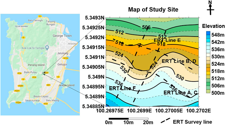
FIGURE 1. Location map of the study site.

Precipitation Data in the Study Area

Precipitation data for the locality (Penang Island) were obtained from the National Centers for Environmental Information station at Penang International, MY. The data were remotely sensed at the Penang International station with position coordinates of latitude and longitude 5.297°, 100.277° at an elevation of 3.4 m and data coverage of about 60% which has a network ID of GHCND:MYM00048601. Table 1 shows global monthly rainfall data obtained from January 2019 to October 2019 with no recorded data for November and December of that year. Similar data have been used in the past for daily precipitation climate data record from multisatellite observations for hydrological and climate studies (Ashouri et al., 2015).

TABLE 1. Summary of precipitation data of the months for the year 2019 and January–March 2020.

Electrical Resistivity Tomography Data Acquisition

ERT field surveys require a high level of technical organization as the electrodes’ position in the survey lines must be colinear (Boyle et al., 2018). Since the study site terrain is a slope with highs and lows, survey lines were perfectly open by cutting the bushes to make a straight line. ERT survey measurements were conducted in November 2019 and January 2020. The first survey was conducted after the end of a period of months of heavy rainfall to allow the ground to be fully saturated. Then, the second and third surveys were conducted during a warmer period when the ground is not wet from lesser rainfall. The ERT survey was conducted using ABEM SAS 4000 Tetrameter connected to Selector ES 464 (4 Channel) and two 100 m cable rolls with 41 electrodes (1.5 m spacing) (Figure 2). The electrodes made of stainless steel of 12 cm long and 1 cm thick were used for data acquisition using an electrode spacing of 1.5 and 60 m survey length with a depth of investigation of approximately 11 m because the depth of investigation is a function of electrode spacing (Park et al., 2017). The choice of electrode spacing was due to some local constraints—shrines and fences—in the study location which do not give room for longer survey lines. The depth of investigation is also limited to 11 m because the record of depth of past landslides in the area is within 2–5 m (Lateh et al., 2011). ERT surveys were conducted in north–south direction downslope and east–west direction perpendicular to the slope in the study site (Figure 1). During ERT measurements in November 2019, five electrodes were excluded due to equipment’s malfunctioning which reduces the number of data points collected. Popular among array configuration used in slope problems by researchers are Wenner, Schlumberger, dipole–dipole, and Wenner–Schlumberger (Metwaly and Alfouzan, 2013; Chalupa et al., 2018; Hojat et al., 2019). These electrode array configurations have their advantages and disadvantages. The choice of the array used depends on depth of penetration, signal strength, and resolution (Reynolds, 1997; Pasierb et al., 2019). Wenner–Schlumberger array configuration was adopted for this study because it is sensitive to both vertical and horizontal changes in the subsurface, thereby able to delineate faults and bedding discontinuities. It has a good resolution, moderate depth of investigation, and signal strength. However, Wenner has a high signal-to-noise ratio but low depth of investigation, and dipole–dipole also has good depth of penetration but poor resolution (Chalupa et al., 2018). The acquired ERT data were inverted with RES2DINV software. However, bad data points were first removed before the inversion process. Robust inversion method with standard data constraint was adopted to reduce the occurrence of very high or very low resistivity values at the sides of the model, but mesh refinement was not reduced to half of the electrode spacing in model discretization. A smoothness-constrained least squares method was used for the inversion (Loke and Barker, 1996). The inversion process converted measured resistance values to apparent resistivity (AR) from the ratio of voltage (potential difference) and current injected to the ground multiplied by the Wenner–Schlumberger geometric factor. The model data have fairly good results after three iterations of the inversion with higher RMS errors ranging from 70% to 71% for ERT data acquired in November 2019, while RMS errors ranging from 18% to 26% for ERT data acquired in January 2020. The disparity between apparent resistivity RMS errors and structures in ERT data acquired in November 2019 and January 2020 can be explained with two limitations of the resistivity method: 1) electrode position and 2) smoothing. First, the survey site is highly vegetated and steep slope which is rapidly undergoing both surface and internal erosion that has adversely affected the landscape and, consequently, the electrode position. Secondly, the ERT data acquired in November 2019 were noisy with high apparent resistivity values close to the surface due to the faulty equipment which also caused reduction of data points. The noise introduces bad data points because of the high apparent resistivity values recorded close to the surface that needs to be removed which leads to lesser data points. A total of 26 misfits were removed from profile A data and 16 misfits from profile B data. These bad data points were more widespread and random at shallow depth close to the surface. Therefore, to produce a smooth model from the ERT data, RES2DINV program allows for the modification of damping factor parameter by increasing it. The damping factor controls the weight given to the model smoothness in the inversion process. However, a larger damping factor produces the model with less structure and poorer resolution because the larger the damping factor, the smoother will be the model, but the apparent resistivity RMS error will be higher or larger (Loke et al., 2013). However, smaller RMS errors do not always imply a more realistic model as more iterations will eventually overfit the model to the data (Hauck and Vonder-Mühll, 2003).

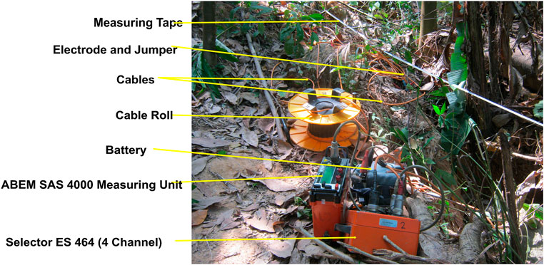
FIGURE 2. Fieldwork data acquisition: fieldwork data acquisition materials ABEM SAS 4000 Tetrameter connected to Selector ES 464 (4 Channel) and cables with electrodes.

Geotechnical Laboratory Tests

The distribution of ERT model values serves as guide to locate the exact depth for the collection of both disturbed and undisturbed soil samples in the study site for geotechnical calibration of ERT results. Samples were taken between 0.1 and 1 m depth from different locations on the profiles C, D, E, and F. These profiles C, D, E, and F have less noise close to the surface with one misfit in profile C and four misfits in profiles D, E, and F. These samples were collected to calibrate ERT model values to know the soil properties or type corresponding to the resistivity value displayed on the model result. The following parameters—moisture content, particle-size distribution, density, and hydraulic conductivity—were determined from the collected samples.

Moisture Content

Soil samples were collected with hand auger at various depths from 0.1 to 1 m and properly weighed to 0.01 g. The weighed samples were placed in an oven to dry with temperature set to 110°C for 24 h and repeatedly weighed until a constant weight is achieved (Olabode and Ocho, 2018). The samples were removed from the oven after drying and allowed to cool and weighed again.

where W1 = weight of the empty can, W2 = weight of the empty can + wet soil sample, W3 = weight of the empty can + dry sample after 24 h in oven.

Particle-Size Distribution

Collected disturbed samples were oven-dried, and sieve analysis was performed on the dry samples. The sieve size was selected based on Wentworth (1922) grain-size classification. The British Standard BS 410/1986 standard number of sieve sizes was adopted for the analysis (Table 2). The sieve was first clean and weighed each to 0.01 g. The selected test soil samples (oven dry soils) were broken to individual particles with the fingers and a rubber-tipped pestle and mortar and poured into the topmost of the nest of selected sieves to be sieved through using a mechanical shaker (Figure 3) for 10 min. Each sieve was weighed to 0.01 g with the soil retained on it. Percentage mass retained was plotted against the sieve size to obtain the particle-size distribution curve.

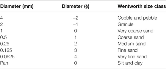
TABLE 2. Selected sieve sizes based on grain-size classification.

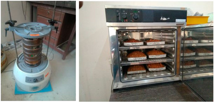
FIGURE 3. A mechanical shaker and oven-dried soil samples.

Density

A calibrated cylindrical steel core cutter container of known weight, length, and diameter (Figure 4A) was used to collect undisturbed soil samples at 0–1 m depth (see Table 4), and the collected soil samples were carefully wrapped with cellophane paper to prevent soil moisture from escaping (Figure 4B). The samples were weighed to 0.01 g in the laboratory after collection. Then, the soil samples were removed from the core container after the mass has been obtained by deducting the weight from the empty steel core cutter weight. The samples were oven-dried for 24 h to a constant weight and then reweighed.

and

FIGURE 4. (A) Calibrated cylindrical steel core cutter containers. (B) Undisturbed soil samples were collected and carefully wrapped with cellophane paper for density determination.

Laboratory Determination of Hydraulic Conductivity

Undisturbed soil samples were collected for permeability tests with a calibrated core cutter cylindrical steel container of known weight, length, and diameter. The samples were carefully wrapped with cellophane paper to prevent soil moisture from escaping. They were weighed to 0.01 g in the laboratory after collection. Constant head and falling head permeability test were both performed on the different samples according to their densities (Figures 5A,B). Sample A is a coarse soil of higher density than sample B which has a higher proportion of fine-grained particles and less dense. Then, from Darcy’s law, the coefficient of permeability for coarse soil was determined by constant head permeability test as follows:

where k is the coefficient of permeability (m/s), q is the total rate of flow or discharge volume (m³), t is the time (s), A is the cross-sectional area (m²), and l is the length of the specimen (m).

FIGURE 5. (A) Constant head permeability test and (B) falling head permeability test experimental setup.

Also, the coefficient of permeability for fine soil was determined by falling head permeability test as follows:

where k = coefficient of permeability (m/s), a is the area of the standpipe (m²), A is the area of the soil sample (m²), l is the length of the soil sample (m), $\Delta t$ is the time for standpipe head to decrease from $h_o$ to $h_1$. Precaution was taken to ensure that both samples were fully saturated and deaired.

Results

Electrical Resistivity Tomography

The analysis of rainfall data shows that the total amount of maximum monthly rainfall was observed in the month of May with a value of 439.42 mm, while the least amount of rainfall was observed in the month of February with a value of 8.13 mm. The maximum amount of rainfall recorded in a day was 152.4 mm in April, whereas the minimum amount of rainfall recorded in a day was 5.08 mm in February. The recorded monthly amount of rainfall was 273.56 mm in the month of October preceding the month of November when the first investigation was carried out. There was no rainfall two days prior to the survey although the ground was still moist and the air temperature of the day of survey was 28°C less than the mean maximum recorded temperature for the year. The mean maximum temperatures occur in the month of April and July with values of 33.8°C and 32.7°C, respectively.

Table 3 shows the characteristics of the six ERT profiles that were acquired using 41 steel electrodes with 1.5 m electrode spacing and a total length of 60 m using Wenner–Schlumberger array configuration. The objective was to obtain models with maximum depth of investigation greater than the average depth of past landslides in the study area. The choice, of array configuration, electrode spacing, and profile length, is to obtain better resolution and maximum depth of investigation. It is moderately sensitive to both horizontal and vertical structures to provide detailed information for monitoring unstable zones in weathered basement rocks that can cause possible movements to provide early warning of future landslides. Therefore, the obtained shallow maximum depth of investigation of 11.1 m (Table 3) is based on the past known occurrences of landslide information in the study area, which occurs within the shallow depth of 2–5 m (Lateh et al., 2011).

TABLE 3. Characteristics of the six electrical resistivity tomography (ERT) profiles acquired using 42 steel electrodes with Wenner–Schlumberger array.

The results of ERT models show the range of resistivity values from 191 to 10,000 Ωm in the six inverted ERT model profiles from November 2019 to January 2020 (Figure 6). ERT model results for profile lines A and B (Figure 6) were acquired in the east–west directions across the study site during the end period of the raining season on November 13, 2019, when the soil is still moist for easy penetration and good contact of the electrode with the soil. Profile line A is situated in the uphill of the slope at the southern part of the study site (see Figure 1), and it is separated by 14 m from profile line B in the downslope toward the north end of the study site. At the central part of profile line A, a distinctive hemispherical low resistivity <600 Ωm is visible below 5 m depth covering an horizontal distance of about 8 m, and it bears resemblance to the low-resistivity hemispherical body displayed in profile line B with the same resistivity values of <600 Ωm within the same depth of 5 m and below but relatively larger covering a horizontal distance of about 10 m. Low-resistivity earth materials of <600 Ωm within 0–5 m depth were observed and identified between 0 and 30 m along both profile lines A and B in the part of the survey lines. Three of such low-resistivity earth materials were observed between the distance of 0 and 21 m within 0–5 m depth in a matrix of high-resistive body of resistivity values greater than >5,000 Ωm in the eastern part of profile line A, whereas four were observed between the same distance and depth in profile line B in the same direction. Another prominent low-resistivity hemispherical earth material was also centrally situated between the horizontal distance of 25 and 30 m and 0–5 m depth within erosional gully along both profile lines A and B. Also, an elongated oval body situated in the west between a profile length of 36 and 40 m within 0–5 m depth with resistivity values greater than >4,000 Ωm is bounded on the top and bottom with materials of resistivity values ≤ 1,350 Ωm. Conversely, a low-resistivity earth material is situated within an horizontal distance of 36–45 m below 5 m depth with resistivity values less than <600 Ωm in profile lines A and B, respectively. High-resistivity contrasts are generally observed between 0 and 12 m along the profiles and in the 24 m mark on both profile lines A and B.

FIGURE 6. Model results of the acquired electrical resistivity tomography data at different dates using Wenner–Schlumberger array configuration: (A,B) profiles in east–west direction on November 13, 2019; (C,D) profiles in east–west direction on January 22, 2020; and (E,F) profiles in north–south direction on January 23, 2020.

On January 22, 2020, the second phase of ERT data were acquired on the same profile lines A and B as C and D (Figure 6). The ERT model results for profile lines C and D were acquired with a protocol different from that of profile lines A and B but with the same array configuration of Wenner–Schlumberger because the former protocol produced data with a large number of misfits and noise. The major difference is that profile lines C and D have more data points than profile lines A and B. A low-resistivity body of <600 Ωm in the bottom layer below 5 m depth is only visible in profile D tomography which extends from the central toward west with an extent length of several tens of meters about 30 m, whereas profile C tomography shows a high-resistivity contrast within the same zone and a low-resistivity hemispherical body of <600 Ωm in the west. At 7 m along the profiles from east are observed low-resistivity materials of resistivity values < 600 Ωm within 0–5 m depth in both profile lines C and D, and it is also observable as an oval shape body at 41 m underneath a high-resistive body of resistivity values > 4,000 Ωm. High-resistivity contrast is visible in both profile lines C and D at 19 m along the profiles within a matrix of the high-resistivity body of resistivity values >5,000 Ωm. Also, two high-resistivity bodies with resistivity values > 4,000 Ωm are displayed in central and western parts of the profile D at 29 m and 44 m, respectively.

ERT model results in Figures 6E,F were both acquired on January 23, 2020, in the north–south direction perpendicular to the profile lines A and B in the study site. They were acquired using the same protocol in profile lines C and D. Along profiles E and F, there are visible centrally elongated body materials oriented in east–west direction with resistivity values <600 Ωm in profile F, while it ranges in values from <600 to 1700 Ωm in profile E and generally below 5 m depth. High-resistivity contrast was observed in the uphill side between 9 and 12 m mark from 0 along profile E within homogeneous resistivity values > 5,000 Ωm in the southern part of the study site. An isolated elongated cylindrical-like body of resistivity values > 4,000 Ωm is also visible toward the north in the downslope end within a relatively homogeneous materials with a resistivity value of about 3,000 Ωm in 0–5 m depth. Also, high-resistivity homogenous materials with resistivity values > 5,000 Ωm which extends for several meters occupied the southern uphill side in profile F within 0–5 m depth, and lenses of the same materials are found scattered within the same depth toward the downslope in the northern end.

Geotechnical Results

The geotechnical parameter test results conducted are summarized in Table 4. It shows the results of moisture content, particle-size distribution, density, and hydraulic conductivity. The estimated moisture content ranges in values from 11.4% to 38.3% (Table 4). Particle-size distribution results for four samples revealed soils with larger percentages of silts and clays that were greater than 20% and very coarse sand, coarse sand, and medium sand greater than 25% (Figure 7). However, the remaining three samples have lower percentages of silts and clays that were less than 20% and very coarse sand and coarse sand greater than 25% (Figure 7). Estimated bulk density ranges from 1,501 to 1781 kg/m³, whereas dry density estimated ranges from 1,176 to 1,458 kg/m³. Density values show relationship with the resistivity values in the study location as revealed in Table 5. Figure 8 shows the relationship that exists between resistivity and density from the study site. Computed hydraulic conductivity value using constant head permeability test was 1.34 × 10⁻² m/s, while falling head permeability test gave a lower value of 2.02 × 10⁻⁵ m/s.

TABLE 4. Summarized geotechnical parameter test results.

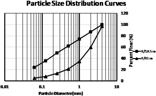
FIGURE 7. Typical particle-size distribution curves in the study site.

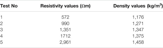
TABLE 5. Result of calculated density values and model resistivity values at designated location.

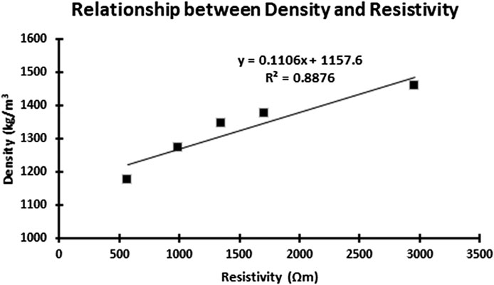
FIGURE 8. Relationship between density and resistivity in the study location.

Discussion

Electrical Resistivity Tomography Models Interpretation

The inverted ERT models were interpreted on the scale of resistivity values that were classified into zones as shown in Table 6. The table shows both weathered and unweathered basement and its spatial distribution of resistivity values into saturated zones with resistivity values ranging from 1 to 600 Ωm, weak zones with resistivity values ranging from 600 to 3,000 Ωm, and basement rock of resistivity value > 5,000 Ωm (Palacky, 1987; Reynolds, 1997; Ghazali et al., 2013).

TABLE 6. Classification of ERT-inverted models on the scale of resistivity values into zones.

Low-resistivity areas with resistivity values <600 Ωm on the ERT models were interpreted as saturated zones in Figure 9. Saturated zones as referred to in this context does not mean zone of saturation below water table but a zone where all the pores are filled with water. Saturated zones identified on the surface (Figures 9A,B,D) occurring within 0–5 m depth may become unstable areas of instability during heavy and continuous rainfall when the ground is completely soaked with water causing the soil to lose its fabric and strength that will result in the sliding of the soil mass. Conversely, saturated zones occurring below 5 m depth (Figures 9D–F) are characterized by possible collapse as a result of subsidence from increase in the soil moisture during continuous rainfall. The boundary between the saturated zones and the high-resistivity overburden materials, which are coarse sand (Table 4), can be defined as the slip surface for movement where landslide can probably occur for the movement of the materials downslope.

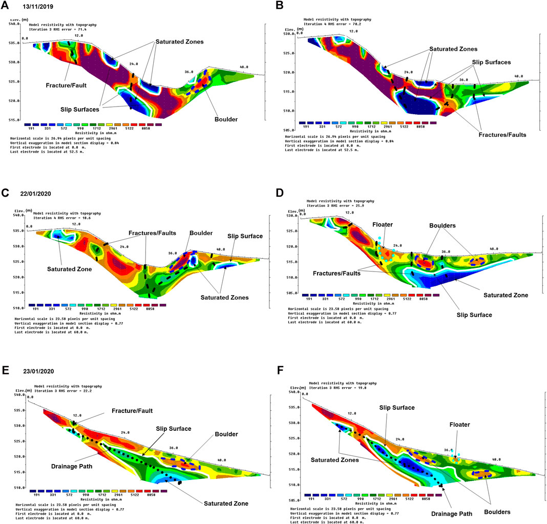
FIGURE 9. Electrical resistivity tomography model interpretation of the acquired data at different dates using Wenner–Schlumberger array: (A,B) profiles in east–west direction on November 13, 2019; (C,D) profiles in east–west direction on January 22, 2020, and (E,F) profiles in north–south direction on January 23, 2020.

High-resistivity contrast indicated by black dash lines (Figure 9) interpreted as faults/fractures were weak zones of instability occurrence because fracture/fault is one of the major causes of slope instability and failure (Martínez et al., 2019; Porres-Benito et al., 2016). Fracture allows vertical flow of soil water and caused a rapidly downward infiltration of soil water during dry period when there is little or no precipitation (Kotikian et al., 2019). We also observed that the study site is a highly fractured/faulted zone as interpreted in Figure 9, and these zones of highly fractured/faulted are usually unstable areas that may be subjected to instability (Andresen, 2018; Raghuvanshi, 2019). Also, high-resistivity materials of resistivity values > 4,000 Ωm that are exposed in the surface as outcrops were interpreted as floaters with curve-dashed cyan line in Figures 9D,F. There is also presence of high resistivity >4,000 Ωm located beneath the surface interpreted as boulder indicated with dashed blue line in Figure 9. Saturated zones were located beneath and beside some of these boulders (Figures 9C–F), which may induce movement during heavy and prolong rainfall (Nordiana et al., 2018a). The continuous infiltrated of water from the prolong rainfall will lead to oversaturation of the cohesive soils within the saturated zones, and it can cause a reduction in the cohesive forces of the soils resulting in the soil particles to be separated from each other by a small infinitesimal distance delta x, and when this happened, their shear strength will not be fully contributed by cohesive force but by internal friction. As soon as this happened, the weight of the boulder will press the material down causing a displacement and movement resulting in the body sliding down the slope. These features may be the triggering factors for future occurrences of landslide in the study site.

Lastly, the low-resistivity materials in Figures 9D–F, which were indicated by a white line is the zone of instability and interpreted as a slip surface for landslide. The dashed black line (Figures 9E,F) is interpreted as the drainage path for the underground water flow. Drainage path is a region where failure is initiated in slope because the water flowing through this path can initiate soil internal erosion referred to as soil pipe. Internal erosion such as piping has been responsible for most landslides occurring in the world as reported by several researchers (Carrazza et al., 2016; Okeke and Wang, 2016; Bernatek-Jakiel and Poesen, 2018). Resistivity values > 5,000 Ωm were interpreted as basement rock without cracks or openings.

Geotechnical Interpretation

High moisture content of 38.3% was recorded from the sample taken at a distance of 10.5 m and 0.1–0.3 m depth (Table 4) with gray color and resistivity value of 1,000 Ωm in Figure 9E on January 24, 2020, whereas the same material sampled at the same point on March 2, 2020, recorded lower percentage value of 28.8%, thus indicating decrease in rainfall and rapid infiltration. Rapid infiltration is an indication of the presence of loose unconsolidated material. The result of geotechnical tests (Table 4) revealed that the highest moisture content of 30.1% was obtained for soil samples collected on March 2, 2020, at a distance of 7 m and 0.8–1 m depth in Figure 9D, and the lowest experimental estimated density and hydraulic conductivity were also obtained as 1,176 kg/m³ and 2.02 × 10⁻⁵ m/s, respectively, with the highest proportion of 31% fine-grained particles of silt and clay that was interpreted as low permeable fine-grained compressible soil (Elhakim, 2016; Kozlowski and Ludynia, 2019; Zhang et al., 2020) that helps to validate the saturated zones identified on the ERT model as low-resistivity values of <600 Ωm. These properties are similar to cohesive materials of high proportion of fine-grained particles because electrical resistivity has the advantage of detecting clay content (cohesive soil) as a very low-resistivity zones (Suzuki et al., 2000), which are usually unstable weak zones of failure. Saturated zones (Figures 9A,B) occurring in the 0–5 m depth will slide downslope when fully saturated during prolong heavy rainfall because the soil water will cause the soil to lose its cohesion which will induce movement (Carrazza et al., 2016; Ghazali et al., 2013). However, the lowest percentage of 11.4% was also obtained for soil sample collected at 41 m in Figure 9F with the highest estimated density and hydraulic conductivity obtained as 1,458 kg/m3 and 1.34 × 10⁻² m/s, respectively, with the lowest percentage of 5% silt and clay. It also validates the weak zones identified on the ERT model as yellow color and interpreted as sand and gravel with a resistivity value of 3,000 Ωm that suggests a permeable loose unconsolidated coarse grain material with a small amount of fine-grained particles (Shelton, 2005) that may be susceptible to soil liquefaction and piping (Carrazza et al., 2016). The particle-size distribution reveals two major types of soils which are coarse sand and sandy loam based on Wentworth (1922) classification. The experimental determined dry densities for samples collected on March 2, 2020, in Table 4 which shows an increasing order of density values for the ERT model resistivity values from the less dense (blue color) to the most dense (yellow color), and hydraulic conductivity values for dense and less dense materials are 1.34 × 10⁻² m/s and 2.02 × 10⁻⁵ m/s, respectively, suggesting that the ERT model is correct which was calibrated by the geotechnical parameters. Table 5 shows the results of density values determined corresponding to the model values at a given depth as shown in Table 4. There is a strong correlation of R = 0.94 between the two variables as shown in Figure 8, suggesting that one variable can be used to predict the other. It can be concluded based on this study that low-resistivity saturated zones are composed of less-dense low-permeable materials, whereas high-resistivity weak zones are composed of more-dense high-permeable materials.

Therefore, identified low-resistivity zones on the ERT models are unstable areas which are inimical to failure because they are composed of weak and compressible incompetent earth materials which tend to yield to failure under stress (Fell et al., 2000), and these zones of instability are where landslide or slope failure can be initiated. Early identification of these zones of instability during slope monitoring may help to predict and provide early warning for future occurrence of landslide or slope failure.

Conclusions

ERT surveys and geotechnical tests have been conducted on the slope of weathered basement of fine-medium-grained granitic rocks in Sungai Ara area of Penang Island hills. Six ERT profiles were acquired between November 2019 and January 2020 at different elevations along the slope site. Two ERT profiles were acquired in November 2019, while the remaining four ERT profiles were acquired in January 2020. The ERT data were inverted using RES2DINV to ERT models. Geotechnical tests and analysis were also carried out on soil samples in the laboratory to obtain soil moisture content, particle-size distribution, density, and hydraulic conductivity.

Analyzed ERT-inverted models were classified on the scale of resistivity values into saturated zones, weak zones, and basement rock. The saturated zones are low-resistivity areas with values < 600 Ωm, which constitute a material of high-water retention having its pores filled with water that may become unstable areas during heavy and prolong rainfall which may cause the soil to lose its fabric, thereby yielding failure. Two zones of instabilities were identified and delineated on the ERT model within 0–5 m depth and 6–11 m depth for near surface and subsurface, respectively. The slope instability identified at the surface or near surface occurs within 0–5 m depth from the surface and is prominent in the uphill in the southern part of the study site, while the subsurface ones occur below 5 m depth in the downslope at the northern part. Weak zones are fracture planes which are usually unstable areas that can be subjected to instability. The near surface instabilities have slip surfaces through which materials can slide, whereas the subsurface instabilities are prone to subsidence. Also, features such as floaters and boulders overlying saturated zones were identified on the ERT model as areas prone to instability which can induce movement during heavy and continuous rainfall as a result of reduction in the cohesive forces within the soil particles resulting in low cohesion and shear strength of the soil materials within the saturated zones. Drainage path was identified as a region where failure can be initiated in slope because the water flowing through this path can initiate soil internal erosion referred to as soil pipe. These features act as triggering factors of landslide, and they were identified on the ERT model as factors responsible for slope instability in weathered basement rock of Penang Island hills.

The geotechnical test revealed that low-resistivity areas with resistivity values < 600 Ωm on the ERT model comprise of high proportion of fine-grained low-permeable compressible cohesive soils, whereas high-resistivity areas with resistivity values ranging from 1,350 to 3,000 Ωm have low proportion of fine-grained high-permeable coarse soils. The identified compressible cohesive soils are prone to slope instability because it can induce displacement or movement when fully saturated during prolong heavy rainfall because the soil water will cause the soil to lose its fabric (cohesive force). The geotechnical test result also revealed a direct relationship between density and resistivity with a strong correlation of R = 0.94 existing between the two variables in the study location. The geotechnical result was able to calibrate the ERT model correctly because low-resistivity materials are less dense and show low hydraulic conductivity, whereas high-resistivity materials are denser with higher hydraulic conductivity based on this study. Therefore, identified low-resistivity areas in the ERT models are unstable zones which are inimical to failure because they are the zones of instability where landslides can be initiated. Early identification of these zones of instability during slope monitoring may help to predict and provide early warning for future occurrence of landslides.

Data Availability Statement

The raw data supporting the conclusions of this article will be made available by the authors, without undue reservation.

Author Contributions

Conceptualization, OO; methodology, OO; software, OO; formal analysis, OO; investigation, OO; resources, LS and MR; data curation, OO; writing–original draft preparation, OO; writing–review and editing, OO; supervision, LS and MR; project administration, OO; funding acquisition, LS. All authors read the manuscript.

Funding

This work is financially supported by the grant “Burning in the Southeast Asian Maritime Continent: Solving Smoke Direct and Semi-Direct Radiative Forcing Through AERONET and MPLNET Constraint” (1001.PFIZIK.8011079), which is under the Research University Grants (RUI) grant from Universiti Sains Malaysia (USM) and Federal University Oye-Ekiti who is responsible for the payment of O. P. Olabode’s salary.

Conflict of Interest

The authors declare that the research was conducted in the absence of any commercial or financial relationships that could be construed as a potential conflict of interest.

Acknowledgments

We would like to thank M. M. Nordiana for her precious advice and comments on this work. We also thank Shahil and other technical staff of Geophysics section, School of Physics, and Zabidi and other technical staff of Geotechnical laboratory, Civil Engineering Department, School of Engineering, Universiti Sains Malaysia (USM). Thanks also go to my colleagues that assisted in the fieldwork exercises. All supports from USM and various parties are gratefully acknowledged. We also acknowledge that the precipitation data used in this research were obtained from National Centers for Environmental Information, and the rainfall information was extracted from the webpage of Department of Irrigation and Drainage, Ministry of Environment and Water, Malaysia.

Supplementary Materials

The Supplementary Material for this article can be found online at: https://www.frontiersin.org/articles/10.3389/feart.2020.580230/full#supplementary-material.

References

Abidin, M. H. Z., Madun, A., Tajudin, S. A. A., and Ishak, M. F. (2017). Forensic assessment on near surface landslide using electrical resistivity imaging (ERI) at Kenyir Lake area in Terengganu, Malaysia. Procedia Eng. 171, 434–444. doi:10.1016/j.proeng.2017.01.354
Ahmad, F., Yahaya, A. S., and Farooqi, M. A. (2006). Characterization and geotechnical properties of penang residual soils with emphasis on landslides. Am. J. Environ. Sci. 2 (4), 121–128. doi:10.3844/ajessp.2006.121.128
Ali, M. M., Ahmad, F., Yahaya, A. S., and Farooqi, M. A. (2011). Characterization and hazard study of two areas of penang Island, Malaysia. Hum. Ecol. Risk Assess. 17 (4), 915–922. doi:10.1080/10807039.2011.588156
Andresen, M. L. (2018). Regional structural analysis of rock slope failure types, mechanisms and controlling bedrock structures in Kåfjorden, Troms. Issue E-Thesis. Norway: Department of Geosciences, The Artic University of Norway Available at: http://hdl.handle.net/10037/12887.
Angelis, D., Tsourlos, P., Tsokas, G., Vargemezis, G., Zacharopoulou, G., and Power, C. (2018). Combined application of GPR and ERT for the assessment of a wall structure at the Heptapyrgion fortress (Thessaloniki, Greece). In J. Appl. Geophys. 152, 208–220. doi:10.1016/j.jappgeo.2018.04.003
Ashouri, H., Hsu, K. L., Sorooshian, S., Braithwaite, D. K., Knapp, K. R., Cecil, L. D., et al. (2015). PERSIANN-CDR: daily precipitation climate data record from multisatellite observations for hydrological and climate studies. Bull. Am. Meteorol. Soc. 96 (1), 69–83. doi:10.1175/BAMS-D-13-00068.1
Askarinejad, A., Akca, D., and Springman, S. M. (2018). Precursors of instability in a natural slope due to rainfall: a full-scale experiment. Landslides 15 (9), 1745–1759. doi:10.1007/s10346-018-0994-0
Baharuddin, I. N. Z., Omar, R. C., Roslan, R., Khalid, N. H. N., and Hanifah, M. I. M. (2016). Determination of slope instability using spatially integrated mapping framework. IOP Conf. Ser. Mater. Sci. Eng. 160 (1), 012080. doi:10.1088/1757-899X/160/1/012080
Baroň, I., and Supper, R. (2013). Application and reliability of techniques for landslide site investigation, monitoring and early warning-Outcomes from a questionnaire study. Nat. Hazards Earth Syst. Sci. 13 (12), 3157–3168. doi:10.5194/nhess-13-3157-2013
Baum, R. L., Godt, J. W., and Savage, W. Z. (2010). Estimating the timing and location of shallow rainfall-induced landslides using a model for transient, unsaturated infiltration. J. Geophys. Res. 115 (3). F03013, doi:10.1029/2009JF001321
Bernatek-Jakiel, A., and Poesen, J. (2018). Subsurface erosion by soil piping: significance and research needs. Earth Sci. Rev. 185 (8), 1107–1128. doi:10.1016/j.earscirev.2018.08.006
Bordoni, M., Valentino, R., Meisina, C., Bittelli, M., and Chersich, S. (2018). A simplified approach to assess the soil saturation degree and stability of a representative slope affected by shallow landslides in oltrepò pavese (Italy). Geosciences 8 (12), 472. doi:10.3390/geosciences8120472
Boyle, A., Wilkinson, P. B., Chambers, J. E., Meldrum, P. I., Uhlemann, S., and Adler, A. (2018). Jointly reconstructing ground motion and resistivity for ERT-based slope stability monitoring. Geophys. J. Int. 212 (2), 1167–1182. doi:10.1093/gji/ggx453
Brillante, L., Mathieu, O., Bois, B., Van Leeuwen, C., and Lévêque, J. (2015). The use of soil electrical resistivity to monitor plant and soil water relationships in vineyards. Soils 1 (1), 273–286. doi:10.5194/soil-1-273-2015
Carrazza, L. P., Moreira, C. A., and Helene, L. P. I. (2016). Gully cavity identification through electrical resistivity tomography. Rev. Bras. Geofís. 34 (2), 241–250. doi:10.22564/rbgf.v34i2.799
Cavalcanti, M. M., Rocha, M. P., Blum, M. L. B., and Borges, W. R. (2018). The forensic geophysical controlled research site of the University of Brasilia, Brazil: results from methods GPR and electrical resistivity tomography. Forensic Sci. Int. 293, 101.e1–101.e21. doi:10.1016/j.forsciint.2018.09.033
Chae, B. G., Park, H. J., Catani, F., Simoni, A., and Berti, M. (2017). Landslide prediction, monitoring and early warning: a concise review of state-of-the-art. Geosci. J. 21 (6), 1033–1070. doi:10.1007/s12303-017-0034-4
Chalupa, V., Pánek, T., Tábořík, P., Klimeš, J., Hartvich, F., and Grygar, R. (2018). Deep-seated gravitational slope deformations controlled by the structure of flysch nappe outliers: insights from large-scale electrical resistivity tomography survey and LiDAR mapping. Geomorphology 321 (08), 174–187. doi:10.1016/j.geomorph.2018.08.029
Chandarana, U. P. (2016). Monitoring and predicting slope instability: a review of current practices from a mining perspective. Int. J. Renew. Energy Technol. 05 (11), 139–151. doi:10.15623/ijret.2016.0511026
Chien, L. K., Hsu, C. F., and Yin, L. C. (2015). Warning model for shallow landslides induced by extreme rainfall. Water (Switzerland) 7 (8), 4362–4384. doi:10.3390/w7084362
Choi, K. Y., and Cheung, R. W. M. (2013). Landslide disaster prevention and mitigation through works in Hong Kong. J. Rock Mechanics Geotech. Engg. 5 (5), 354–365. doi:10.1016/j.jrmge.2013.07.007
De Vita, P., Fusco, F., Tufano, R., and Cusano, D. (2018). Seasonal and event-based hydrological and slope stability modeling of pyroclastic fall deposits covering slopes in Campania (Southern Italy). Water (Switzerland) 10 (9), 1140. doi:10.3390/w10091140
Di Traglia, F., Nolesini, T., Ciampalini, A., Solari, L., Frodella, W., Bellotti, F., et al. (2018). Tracking morphological changes and slope instability using spaceborne and ground-based SAR data. Geomorphology 300, 95–112. doi:10.1016/j.geomorph.2017.10.023
Elhakim, A. F. (2016). Estimation of soil permeability. Alexandria Engg. J. 55 (3), 2631–2638. doi:10.1016/j.aej.2016.07.034
Epada, P. D., Sylvestre, G., and Tabod, T. C. (2012). Geophysical and geotechnical investigations of a landslide in Kekem Area , western Cameroon. Int. J. Geosci. 3 (09), 780–789. doi:10.4236/ijg.2012.34079
Eppes, M. C., and Keanini, R. (2017). Mechanical weathering and rock erosion by climate-dependent subcritical cracking. Rev. Geophys. 55 (2), 470–508. doi:10.1002/2017RG000557
Fell, R., Hungr, O., Leroueil, S., and Riemer, W. (2000). “Keynote lecture–Geotechnical engineering of the stability of natural slopes, and cuts and fills in soil,” in ISRM international symposium, international society for rock mechanics, 2000, 100, 2000. November 19–24, Melboure, Australia. Available at: .
https://doi.org/https://www.researchgate.net/publication/267403410 Keynote | Google Scholar
Froude, M. J., and Petley, D. N. (2018). Global fatal landslide occurrence from 2004 to 2016. Nat. Hazards Earth Syst. Sci. 18 (8), 2161–2181. doi:10.5194/nhess-18-2161-2018
Gaffney, V., Neubauer, W., Garwood, P., Gaffney, C., Löcker, K., Bates, R., et al. (2018). Durrington walls and the stonehenge hidden landscape project 2010–2016. Archaeol. Prospect. 25 (3), 255–269. doi:10.1002/arp.1707
Ghazali, M. A., Rafek, A. G., Md Desa, K., and Jamaluddin, S. (2013). Effectiveness of geoelectrical resistivity surveys for the detection of a debris flow causative water conducting zone at KM 9, gap-fraser’s hill road (FT 148), Fraser’s Hill, Pahang, Malaysia. J. Geol. Res. 2013 (2014), 1–11. doi:10.1155/2013/721260
Giocoli, A., Stabile, T. A., Adurno, I., Perrone, A., Gallipoli, M. R., Gueguen, E., et al. (2015). Geological and geophysical characterization of the southeastern side of the High Agri Valley (southern Apennines, Italy). Nat. Hazards Earth Syst. Sci. 15 (2), 315–323. doi:10.5194/nhess-15-315-2015
Gunn, D. A., Chambers, J. E., Dashwood, B. E., Lacinska, A., Dijkstra, T., Uhlemann, S., et al. (2018). Deterioration model and condition monitoring of aged railway embankment using non-invasive geophysics. Construct. Build. Mater. 170, 668–678. doi:10.1016/j.conbuildmat.2018.03.066
Hakro, M. R., and Harahap, I. S. H. (2015). Laboratory experiments on rainfall-induced flowslide from pore pressure and moisture content measurements. Nat. Hazards Earth Syst. Sci. Discuss. 3, 1575–1613. doi:10.5194/nhessd-3-1575-2015
Hauck, C., and Vonder-Mühll, D. (2003). Inversion and interpretation of two‐dimensional geoelectrical measurements for detecting permafrost in mountainous regions. Permafr. Periglac. Process. 14 (4), 305–318. doi:10.1002/ppp.462
Hen-Jones, R. M., Hughes, P. N., Stirling, R. A., Glendinning, S., Chambers, J. E., Gunn, D. A., et al. (2017). Seasonal effects on geophysical–geotechnical relationships and their implications for electrical resistivity tomography monitoring of slopes. Acta Geotechnica. 12 (5), 1159–1173. doi:10.1007/s11440-017-0523-7
Hojat, A., Arosio, D., Ivanov, V. I., Longoni, L., Papini, M., Scaioni, M., et al. (2019). Geoelectrical characterization and monitoring of slopes on a rainfall-triggered landslide simulator. J. Appl. Geophys. 170, 103844. doi:10.1016/j.jappgeo.2019.103844
Hübner, R., Heller, K., Günther, T., and Kleber, A. (2015). Monitoring hillslope moisture dynamics with surface ERT for enhancing spatial significance of hydrometric point measurements. Hydrol. Earth Syst. Sci. 19 (1), 225–240. doi:10.5194/hess-19-225-2015
Intrieri, E., Carlà, T., and Gigli, G. (2019). Forecasting the time of failure of landslides at slope-scale: a literature review. Earth Sci. Rev. 193 (3), 333–349. doi:10.1016/j.earscirev.2019.03.019
Ismail, N. I., and Yaacob, W. Z. W. (2018). Application of electrical resistivity tomography (ERT) for slope failure investigation: a case study from kuala lumpur. Jurnal Teknologi Sci. Engg. 80 (5), 2180–3722. Available at: www.jurnalteknologi.utm.my
Jeong, S., Lee, K., Kim, J., and Kim, Y. (2017). Analysis of rainfall-induced landslide on unsaturated soil slopes. Sustainability 9 (7), 1–20. doi:10.3390/su9071280
Jeong, S. S., Kim, J. H., Kim, Y. M., and Bae, D. H. (2014). Susceptibility assessment of landslides under extreme-rainfall events using hydro-geotechnical model: a case study of Umyeonsan (Mt.), Korea. Nat. Haz. Earth Syst. Sci. Discuss. 2 (8), 5575–5601. doi:10.5194/nhessd-2-5575-2014
Kirschbaum, D., Kapnick, S., Stanley, T., and Pascale, S. (2020). Changes in extreme precipitation and landslides over high mountain asia. Geophy. Res. Lett. 28, e2019GL085347. doi:10.1029/2019GL085347
Kirschbaum, D., Stanley, T., and Zhou, Y. (2015). Spatial and temporal analysis of a global landslide catalog. Geomorphology 249, 4–15. doi:10.1016/j.geomorph.2015.03.016
Kotikian, M., Parsekian, A. D., Paige, G., and Carey, A. (2019). Observing heterogeneous unsaturated flow at the hillslope scale using time‐lapse electrical resistivity tomography. Vadose Zone J. 18 (1), 1–16. doi:10.2136/vzj2018.07.0138
Kozlowski, T., and Ludynia, A. (2019). Permeability coefficient of low permeable soils as a single-variable function of soil parameter. Water (Switzerland) 11 (12), 5–7. doi:10.3390/w11122500
Kumar, A., and Rathee, R. (2017). Monitoring and evaluating of slope stability for setting out of critical limit at slope stability radar. Intl. J. GeoEngg. 8 (1), 18. doi:10.1186/s40703-017-0054-y
Lateh, H., Muqtada, M. A. K., and Jefriza, H. (2011). Monitoring of shallow landslide in Tun Sardon KM 3.9. Int. J. Phys. Sci. 6 (12), 2989–2999. doi:10.5897/IJPS11.118
Loke, M. H., and Barker, R. D. (1996). Rapid least-squares inversion of apparent resistivity pseudosections by a quasi-Newton method1. Geophys. Prospect. 44 (1), 131–152. doi:10.1111/j.1365-2478.1996.tb00142.x
Loke, M. H., Chambers, J. E., Rucker, D. F., Kuras, O., and Wilkinson, P. B. (2013). Recent developments in the direct-current geoelectrical imaging method. J. Appl. Geophys. 95, 135–156. doi:10.1016/j.jappgeo.2013.02.017
Martínez, J., Rey, J., Sandoval, S., Hidalgo, M. C., and Mendoza, R. (2019). Geophysical prospecting using ERT and IP techniques to locate Galena veins. Rem. Sens. 11 (24), 2923. doi:10.3390/rs11242923
Metwaly, M., and Alfouzan, F. (2013). Application of 2-D geoelectrical resistivity tomography for subsurface cavity detection in the eastern part of Saudi Arabia. Geosci. Front. 4 (4), 469–476. doi:10.1016/j.gsf.2012.12.005
Moragues, S., Gabriela Lenzano, M., Moreiras, S., Vecchio, A. Lo., Lannutti, E., and Lenzano, L. (2019). Slope instability analysis in South Patagonia applying multivariate and bivariate techniques on Landsat images during 2001–2015 period. Catena 174, 339–352. doi:10.1016/j.catena.2018.11.024
Nordiana, M. M., Azwin, I. N., Nawawi, M. N. M., and Khalil, A. E. (2018a). Slope failures evaluation and landslides investigation using 2-D resistivity method. NRIAG J. Astron Geophy. 7 (1), 84–89. doi:10.1016/j.nrjag.2017.12.003
Nordiana, M. M., Ghafar, S. H. M. A., Sukr, M. S., and Jinmin, M. (2018b). “Identification of slope failure using 2-D resistivity method,” in Proceedings of academicsera 14th international conference, Osaka, Japan, 9th–10th March 2018.
Okeke, A. C. U., and Wang, F. (2016). Hydromechanical constraints on piping failure of landslide dams: an experimental investigation. Geoenviron. Dis. 3 (1), 4. doi:10.1186/s40677-016-0038-9
Olabode, O, and Ocho, P. I. (2018). 2-D electrical resistivity tomography monitoring of soil moisture distribution in A rain-fed maize plot. FUW Trends Sci. Tech. J. 3 (2A), 430–435. Available at: www.ftstjournal.com.
Palacky, G. V. (1987). “Resistivity characteristics of geologic targets,” in Electromagnetic methods in applied geophysics-theory, society of exploration geophysicists, Tulsa, OK. Editor M. Nabighian, Vol. 1, 53–129. doi:10.1190/1.9781560802631.ch3.
Park, C. S., Jeong, J. H., Park, H. W., and Kim, K. (2017). Experimental study on electrode method for electrical resistivity survey to detect cavities under road pavements. Sustainability 9 (12), 1–21. doi:10.3390/su9122320
Park, S., Lim, H., Tamang, B., Jin, J., Lee, S., Chang, S., et al. (2019). A study on the slope failure monitoring of a model slope by the application of a displacement sensor. J. Sensors. 2019, 7570517. doi:10.1155/2019/7570517
Pasierb, B., Grodecki, M., and Gwóźdź, R. (2019). Geophysical and geotechnical approach to a landslide stability assessment: a case study. Acta Geophysica. 67 (6), 1823–1834. doi:10.1007/s11600-019-00338-7
Porres-Benito, J. A., Ibanez, S. J., Ortiz-Palacio, S., and López-Ausín, V. (2016). “Fractures location on karstified limestone surfaces by electrical resistivity tomography characterization,” in Proceedings of the 5th international conference on geotechnical and geophysical site characterisation, (ISSMGE TC‐102 – ISC'5), ISC 2016, Gold Coast, Queensland, Australia, Semptember 5–9, 2016, Vol. 2, 929–933. Available at: https://www.issmge.org/publications/online-library.
Pradhan, B., and Lee, S. (2010). Delineation of landslide hazard areas on Penang Island, Malaysia, by using frequency ratio, logistic regression, and artificial neural network models. Environ. Earth Sci. 60 (5), 1037–1054. doi:10.1007/s12665-009-0245-8
Raghuvanshi, T. K. (2019). Plane failure in rock slopes–a review on stability analysis techniques. J. King Saud Univ. Sci. 31 (1), 101–109. doi:10.1016/j.jksus.2017.06.004
Reynolds, J. M. (1997). An introduction to applied and environmental geophysics. John Wiley and Son LtdChichester, England. Available at: .
Sajinkumar, K. S., Anbazhagan, S., Pradeepkumar, A. P., and Rani, V. R. (2011). Weathering and landslide occurrences in parts of Western Ghats, Kerala. J. Geol. Soc. India. 78 (3), 249–257. doi:10.1007/s12594-011-0089-1
Shelton, P. D. (2005). The conservation and management of unconsolidated geological sections (Issue Number 563). Available at: http://publications.naturalengland.org.uk/file/93025. (Accessed May 30, 2020).
Shevnin, V., Mousatov, A., Ryjov, A., and Delgado-rodriquez, O. (2007). Estimation of clay content in soil based on resistivity modelling and laboratory measurements. Geophys. Prospect. 55 (2), 265–275. doi:10.1111/j.1365-2478.2007.00599.x
Sidle, R. C., and Bogaard, T. A. (2016). Dynamic earth system and ecological controls of rainfall-initiated landslides. Earth Sci. Rev. 159, 275–291. doi:10.1016/j.earscirev.2016.05.013
Soto, J., Galve, J. P., Palenzuela, J. A., Azañón, J. M., Tamay, J., and Irigaray, C. (2017). A multi-method approach for the characterization of landslides in an intramontane basin in the Andes (Loja, Ecuador). Landslides 14 (6), 1929–1947. doi:10.1007/s10346-017-0830-y
Suzuki, K, Toda, S, Kusunoki, K, Fujimitsu, Y, Mogi, T, and Jomori, A, (2000). Case studies of electrical and electromagnetic methods applied to mapping active faults beneath the thick quaternary. Dev. Geotech. Eng. 84, 29–45. doi:10.1016/S0165-1250(00)80005-X
Tan, B. K. (1994). Engineering properties of granitic soils and rocks of Penang Island, Malaysia. Bull. Geol. Soc. Malaysia. 35 (8), 69–77. doi:10.7186/bgsm35199408
Tang, G., Huang, J., Sheng, D., and Sloan, S. W. (2018). Stability analysis of unsaturated soil slopes under random rainfall patterns. Eng. Geol. 245 (3), 322–332. doi:10.1016/j.enggeo.2018.09.013
Tomás, R., Abellán, A., Cano, M., Riquelme, A., Tenza-Abril, A. J., Baeza-Brotons, F., et al. (2018). A multidisciplinary approach for the investigation of a rock spreading on an urban slope. Landslides 15 (2), 199–217. doi:10.1007/s10346-017-0865-0
Tomecka-Suchoń, S., Zogała, B., Gołȩbiowski, T., Dzik, G., Dzik, T., and Jochymczyk, K. (2017). Application of electrical and electromagnetic methods to study sedimentary covers in high mountain areas. Acta Geophysica. 65 (4), 743–755. doi:10.1007/s11600-017-0068-z
Wang, Y. X., Guo, P. P., Ren, W. X., Yuan, B. X., Yuan, H. P., Zhao, Y. L., et al. (2017). Laboratory investigation on strength characteristics of expansive soil treated with jute fiber reinforcement. Int. J. GeoMech. 17 (11), 1–12. doi:10.1061/(ASCE)GM.1943-5622.0000998
Wei, S., Zhaoguang, H., Ying, G., Chengchang, Z., and Yao, L. (2017). Resistivity model of frozen soil and high ‐ density resistivity method for exploration discontinuous permafrost. In INTECH (Issue May). World’s largest Science, Technology and Medicine. doi:10.5772/intechopen.68197
Wentworth, C. K. (1922). A scale of grade and class terms for clastic sediments. J. Geol. 30 (5), 377–392. doi:10.1086/622910
Whiteley, J. S., Chambers, J. E., Uhlemann, S., Wilkinson, P. B., and Kendall, J. M. (2019). Geophysical monitoring of moisture-induced landslides: a review. Rev. Geophys. 57 (1), 106–145. doi:10.1029/2018RG000603
Winter, M. G., Shearer, B., Palmer, D., Peeling, D., Harmer, C., and Sharpe, J. (2016). The economic impact of landslides and floods on the road network. Procedia Engg. 143, 1425–1434. doi:10.1016/j.proeng.2016.06.168
Yamakawa, Y., Kosugi, K., Masaoka, N., Sumida, J., Tani, M., and Mizuyama, T. (2012). Combined geophysical methods for detecting soil thickness distribution on a weathered granitic hillslope. Geomorphology 145–146, 56–69. doi:10.1016/j.geomorph.2011.12.035
Yang, R., Xiao, P., and Qi, S. (2019). Analysis of slope stability in unsaturated expansive soil: a case study. Front. Earth Sci. 7, 292. doi:10.3389/feart.2019.00292
Keywords: geotechnical properties, electrical resistivity tomography, saturated zones, slope instability monitoring, low-resistivity zones, low-permeable unstable zones
Citation: Olabode OP, San LH and Ramli MH (2020) Analysis of Geotechnical-Assisted 2-D Electrical Resistivity Tomography Monitoring of Slope Instability in Residual Soil of Weathered Granitic Basement. Front. Earth Sci. 8:580230. doi: 10.3389/feart.2020.580230
Received: 21 March 2020; Accepted: 22 September 2020;
Published: 11 November 2020.
Edited by:
uigi JovaneL, University of São Paulo, BrazilReviewed by:
Vagner Roberto Elis, Universidade de São Paulo, BrazilMichael Oladunjoye, University of Ibadan, Nigeria
Copyright © 2020 Olabode, San and Ramli. This is an open-access article distributed under the terms of the Creative Commons Attribution License (CC BY). The use, distribution or reproduction in other forums is permitted, provided the original author(s) and the copyright owner(s) are credited and that the original publication in this journal is cited, in accordance with accepted academic practice. No use, distribution or reproduction is permitted which does not comply with these terms.
*Correspondence: Oladunjoye P. Olabode, olabodeop@student.usm.my, Lim H. San, hslim@usm.my