Automated Processing of Declassified KH-9 Hexagon Satellite Images for Global Elevation Change Analysis Since the 1970s

1. Introduction

The Earth’s surface has evolved dramatically over the last century as a consequence of anthropogenic activities and climate change (IPCC, 2019; IPCC SROC, 2019). But documenting these changes at regional scales over such a time span remains a challenge (James et al., 2012). Digital Elevation Models (DEMs), orthogonally gridded representations of surface elevation, are extremely valuable data for the quantitative study of Earth surface deformation with important applications, e.g., in glaciology, seismology, natural hazards or geomorphology (Tsutsui et al., 2007; Zhou et al., 2016; Anderson, 2019; Shean et al., 2020). Modern high-resolution satellites now provide such data at annual to daily intervals and with sub-meter accuracy (Shean et al., 2016; Porter et al., 2018; Howat et al., 2019). However, prior to the Shuttle Radar Topography Mission (SRTM) in 2000, no elevation data are available at a global scale with the decameter resolution required to study Earth surface deformation. Documenting surface changes prior to year 2000 requires the exploitation of older remote sensing archives, typically from aerial platforms (Kjeldsen et al., 2015; Girod et al., 2018). A potential source of data to fill in the temporal gap is declassified American intelligence satellite imagery, such as from the Corona and Hexagon programs (Galiatsatos et al., 2007; Burnett, 2012; Fowler, 2013). Here we will focus on the Hexagon program.

1.1. The Hexagon Program

The Hexagon program (codename KeyHole-9 or KH-9) consisted of a series of 20 reconnaissance satellites launched in low Earth orbit and operated by the United States during the Cold War from 1972 to 1986 (Burnett, 2012). The program improved upon the successful Corona (KH-1 to 4) satellite missions (1959–1972) to provide the US with high-resolution images of the Earth, in particular to verify Soviet strategic weapons technologies following arms limitation treaties. The primary instruments on the KH-9 satellites were two rotating 60-inch (152.4 cm) focal length panoramic film cameras that acquired images at $\sim$0.8 m ground resolution (Burnett, 2012). The total ground coverage for all KH-9 missions was 789 million km², surveying nearly all of Earth’s land surface multiple times. Twelve of the 20 missions were also equipped with a mapping camera (MC), whose purpose was to provide global cartographic information (Figure 1) and acquire images at 6–9 m resolution (Burnett, 2012). Unfortunately, large areas particularly in Australia, North America, the interior of the ice sheets or at low latitudes were not or insufficiently surveyed by the MC. These twelve missions returned 29,000 MC images on a total of 14 km of film. After image acquisition, the film was stored in capsules (called “buckets”) which were ejected from the satellite, re-entered the Earth’s atmosphere, and slowed via parachutes before being retrieved in midair by an aircraft. Given the high scientific value of the images for global change studies, this imagery was declassified and released to the National Archives and Records Administration (NARA) and the U.S. Geological Survey (USGS) in 2002 (mapping camera) and 2011 (panoramic camera). The USGS archived and indexed the film, and distributes scanned digital copies of images at 7 μm resolution at no cost (or with a nominal fee of $30 for images that have not yet been digitized), available at https://earthexplorer.usgs.gov/. KH-9 MC images offer the advantage of a larger coverage, simpler frame camera optics as opposed to rotating cameras, and presence of reseau markers (see Sections 2.1 and 2.2) compared to other declassified archives. We therefore focus on the processing of the KH-9 MC images in this study.

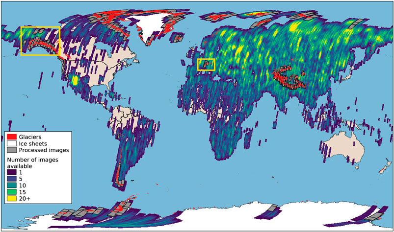
FIGURE 1. Map showing the number of KH-9 MC images available in the USGS archive (color scale), the 698 images preprocessed in this study (gray, Section 2.3), glacier outlines from RGI v6.0 (red), and outlines for the two study areas in Alaska and European Alps (yellow rectangles).

1.2. Relevance for the Study of Changes in Earth Surface

With their high resolution, high quality and open access, the scanned KH-9 MC images comprise one of the best global satellite data sets for the 1970s. Accordingly, the MC archive has attracted a lot of attention in the scientific community. The first scientific references to the data consisted of a qualitative image interpretation to identify archaeological features (Fowler, 2004; Scardozzi, 2008), glacier features (Grant et al., 2009; Narama et al., 2010a; Narama et al., 2010b), landslides (Larsen and Montgomery, 2012) and land-cover change (Kivinen and Kumpula, 2014). The first quantitative processing of the stereo images was performed by Surazakov and Aizen (2010), who revealed the potential of the data to generate historical topography and to study Earth’s surface deformation. Following this study, stereoscopic KH-9 MC images have been widely used to study glacier area change (Bolch et al., 2010; Fujita et al., 2011; Bhambri et al., 2012; Bhambri et al., 2013; Masiokas et al., 2015), glacier elevation change (Pieczonka et al., 2013; Holzer et al., 2015; Maurer and Rupper, 2015; Pieczonka and Bolch, 2015; Lamsal et al., 2017; Zhou et al., 2018; Belart et al., 2019; King et al., 2019; Maurer et al., 2019), landslides (Lacroix et al., 2020) and tectonic deformation (Hollingsworth et al., 2012; Zhou et al., 2016).

1.3. Limitations and Steps Forward for the Processing of the KH-9 Mapping Camera Images

Most aforementioned studies relied on manually intensive identification of Ground Control Points (GCPs) to estimate unknown camera position and orientation, typically for a few selected image pairs. Maurer and Rupper (2015) presented an automated workflow able to process the raw scanned images into a DEM with little manual input by leveraging computer vision algorithms. It enabled them to study glacier elevation changes at basin (Maurer et al., 2016) and regional scales (Maurer et al., 2019) in the very steep and challenging terrain of the Himalayas. However, this processing was developed and tested in areas with relatively small glaciers, with a large availability of stable ground for image co-registration and camera calibration, and on smaller image subsets of about 5,000 × 5,000 pixels (about 72 such subsets make an entire KH-9 MC image). This approach has not yet been tested for terrains with larger glaciers, ice sheets and oceans, such as in the polar regions where exposed ground is sparse, snow cover is predominant, and GCPs are challenging to identify. Additionally, in all previous studies, the intrinsic parameters of the camera (e.g., focal length and lens distortion) were, if at all, estimated for each image subset and not documented. Hence, no general camera model has been published for the KH-9 missions to allow a consistent processing of the entire archive. Finally, the accuracy of the KH-9 MC DEMs in previous studies was rarely validated against ancillary observations, especially over snow- and ice-covered areas, where image saturation and limited contrast introduce major challenges for stereo processing.

Here we present an automated workflow designed to process the scanned KH-9 MC images into DEMs at 24 m posting. A preprocessing step converts the “raw” scanned images into undistorted images suitable for stereo reconstruction. Stereo pairs are then processed automatically using the freely available NASA Ames Stereo Pipeline (Beyer et al., 2018) that now includes the updates implemented for this study (version 2.6.2). The workflow is later referred to as ASPy. We used ASPy to process several hundred image pairs, which enabled us to estimate reliable MC focal length and lens parameters for each KH-9 mission. We validate the estimated camera parameters by processing all scenes available over the European Alps and South coast of Alaska, the latter being particularly challenging due to the prevalence of glaciers and ocean. Finally, we perform a rigorous accuracy assessment for sample DEMs using external elevation data, with a specific focus on ice/snow terrain. We then present an analytical approach to propagate this uncertainty when spatially averaging elevation change estimates (or volume change). Although the processing workflow and accuracy assessment can be used for many applications, we focus our analysis on glaciological applications.

2. Data

2.1. The Mapping Camera System and Acquisition

The mapping camera (MC) acquired images in two stereo modes, bilap and trilap, providing respectively 55 and 70% overlap between consecutive frames (Burnett, 2012). Film were exposed in a single shot with a 12-inch (304.8 mm) focal length camera that provided a field of view of 38° by 72° or a ground footprint of approximately 130 × 260 km. Lens distortion are reported as less than 100 μm (radial) and 20 μm (tangential) (Burnett, 2012, Table 2.5), but detailed camera calibration reports are still unavailable or classified. The satellite ephemeris and attitude were estimated using star field photographs acquired simultaneously with the MC images, a doppler beacon and Navy Navigational System (NAVPAC). While the satellite ephemerides remain classified, the USGS provides approximate image footprints with geolocation accuracy of a few kilometers.

2.2. Image Characteristics

Despite the declassification, many characteristics of the mapping camera and resulting images are poorly documented. Each image includes an array of fiducial markers (dark crosses) spaced every 10 mm that was imprinted by a reseau plate. The number of these reseau markers is 23 in the horizontal direction and 47 in the vertical direction (Maurer and Rupper, 2015) or 1,081 in total (Figure 2). This number was erroneously reported as 1,058 (23 × 46) by Surazakov and Aizen (2010) and referenced many times after that (e.g., Pieczonka et al., 2013; Goerlich et al., 2017). The optical center of the image is located at the center of the reseau grid, and is also often marked by specific reseau markers in the center of each edge. Furthermore, image dimensions in previous studies were reported to be either 9 inches by 18 inches (228.6 mm × 457.2 mm) or 23 cm × 46 cm (Surazakov and Aizen, 2010; Burnett, 2012; Pieczonka et al., 2013). While the length of the reseau grid is exactly 46 cm (ruling out the possibility of a 457.2 mm image length), the dimension of the exposed area was measured manually (with a 1/4-inch division ruler) on a copy of the film visualized at NARA as 9 inches × 18.25 inches (22.86 cm × 46.36 cm). A length of 18.22 inches (46.28 cm) is also reported in declassified document TCS-21037/73.¹ The 10 mm spacing between reseau markers is hence used as a reference for resizing the scanned images throughout the preprocessing.

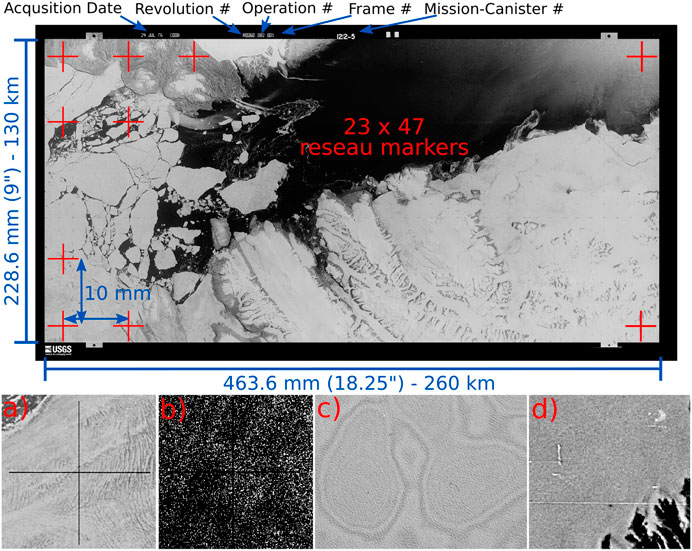
FIGURE 2. Sample KH-9 MC image over the Canadian Arctic (ID DZB1212-500082L001001), after stitching. The image dimensions and metadata information are highlighted in blue. Each image has 23 × 47 reseau markers (dark crosses). Detail of (A) reseau marker with good contrast, (B) reseau marker over water with limited contrast (Digital number stretched from 0–5 to bring out detail, rather than 0–255 as in A), (C) interference pattern known as Newton’s rings, caused by the reflection of light when the film is not in contact with the scanner glass, and (D) scratches and defects on the film.

The USGS scans their copy of the film using a Leica DSW700 scanner (USGS, personal communications), with 7 μm resolution and an 8-bit depth. Two scans are required to capture the $\sim$46 cm frame, and the images are delivered as two TIF files with $\sim$15% overlap. Each image is approximately 35.000 × 35.000 pixels ($\sim$1.2 GB uncompressed).

2.3. Study Areas

We ordered and preprocessed a total of 698 KH-9 MC images, extending over most glacierized areas of the world (Figure 1). We selected in priority images with minimal cloud and snow cover, but also selected images with fresh snow cover or fractional cloud cover for testing or in areas where no optimal images were available. We also included images in coastal areas (in the Arctic and Antarctic), excluded from most studies dealing with KH-9 MC images (see Section 1) that can represent a challenge for the preprocessing and camera calibration. The totality of the images were used to test and develop the preprocessing step (Section 3.1). Among those, we selected 424 images for the estimation of the camera intrinsic parameters (Section 3.2). The selection was based on image quality, the presence of sufficient stable terrain (after excluding glaciers and water bodies) to ensure good conditions for the bundle adjustment and global sampling (central Asia, Europe, Arctic). We further selected a subset of 12 of these images over the European Alps (hereafter referred as “Alps”) and 47 along the south coast of Alaska and parts of Yukon, Canada (hereafter referred as “Alaska”, Figure 1) to evaluate the output DEM accuracy (Section 3.3). The list of these images is provided in Supplementary.

2.4. Ancillary Digital Elevation Models

We used several external DEM products to co-register and evaluate the KH-9 MC DEMs.

For the co-registration of all KH-9 MC DEMs, we used the 30 m posting void-filled Shuttle Radar Topography Mission (SRTM) DEM version 3 (Farr et al., 2007) for low to mid-latitudes (56°S-60°N) and the 32 m ArcticDEM mosaics for areas north of 60° latitude (Porter et al., 2018). These were chosen because of the availbility of DEMs at a resolution as close as possible to our final products (24 m posting). These DEMs were also used for the DEM accuracy assessment.

We used the 90 m TanDEM-X global DEM (Rizzoli et al., 2017) as an additional elevation reference in Alaska. The DEM has an absolute vertical accuracy, at 90% confidence level, of 10 m and a relative vertical accuracy (between adjacent pixels) of 2 m for low and medium relief terrain and 4 m for high relief terrain. Erroneous elevations were filtered using the provided Height Error Map (HEM). Pixels with HEM larger than 0.5 were visually identified as noisy and excluded for this analysis.

For validation over the Alps, we used the SwissAlti3D DEM provided by the Swiss Federal Office of Topography.² This product is a bare ground digital terrain model without vegetation and buildings for all of Switzerland at 2 m posting and a 1-sigma vertical accuracy of 0.5 m (below 2,000 m) or 1–3 m (above 2,000 m).

To validate the KH-9 MC DEMs over evolving glacier surfaces, we used two DEMs acquired within 1 year from the corresponding KH-9 MC images. For the Alaska study area, we used a DEM derived from topographic map elevation contour lines and used in other glaciological studies (Berthier et al., 2010) and sampled at 40 m. A small section covering essentially Walsh and Donjek glaciers and acquired in 1977 was extracted as it was acquired on the same year as some of the KH-9 MC images, and hereafter referred as “Hist 1977.” The uncertainty of this DEM is relatively large compared to the other data set, with a 1σ uncertainty of $\sim$14 m (Figure 8) but it is the best source available for that period. For the Swiss Alps study site, we used a 1 m DEM derived from aerial images acquired in 1980 (Ginzler et al., 2019), with a vertical accuracy of $\sim$2 m (Figure 8). The DEM was downsampled at 24 m resolution using bilinear interpolation, for comparison with the KH-9 DEMs, and hereafter referred as “Hist 1980.”

All ancillary DEMs in a given area are co-registered to a single reference DEM following the approach outlined in (Nuth and Kääb, 2011). We used the SRTM DEM as a reference in the Alps and ArcticDEM in Alaska. Horizontal shifts were always less than a pixel of the reference DEM.

2.5. Land Cover Data

During DEM co-registration (Section 3.2.3), it was necessary to mask water bodies and glaciers (where large changes in surface elevation are expected for this time period). We used the NOAA shoreline data set (Wessel and Smith, 1996) to identify oceans and large lakes and the Randolph Glacier Inventory version 6.0 (RGI Consortium, 2017) to identify glaciers. While both data set are not necessarily representative of our study period, the co-registration process is insensitive to a small number of outliers and the outlines proved sufficient for this step. The RGI outlines generally correspond to glacier extents of the period 2000–2010. While the glacier extent during our study period (1973–1980) are expected to be different (larger for most glaciers), we used the RGI outlines to compute on-ice statistics. Off-ice (or “stable” areas) statistics, on the other hand, were calculated only for pixels beyond a 2 km buffer around the RGI polygons.

For comparison with the other digital surface models that represent the elevation of the surface (including canopy and buildings), urban and forested areas were masked in the SwissAlti3D DEM using the 2012 CORINE land cover from the European Copernicus program (Feranec et al., 2016).

3. Methods

ASPy consists of two main processing stages, described below: a preprocessing stage (Section 3.1) to convert the original scans into a merged, distortion-free image and a stereo processing stage (Section 3.2) to convert stereo pairs into a DEM.

3.1. Image Preprocessing

3.1.1. Reseau Markers Detection

The first preprocessing step is to identify the reseau markers (crosses, Figure 2) to correct for possible distortions of the film introduced during on orbit operations, duplication, 40 years of storage and additional handling during scanning. Detection of the reseau markers is done in a way similar to Maurer and Rupper (2015) with improvements in order to be more robust to outliers and detect even the faintest markers in dark areas, mostly over water (Figure 2B) that were less frequent in the non-coastal images processed in that study. ASPy’s marker detection involves four steps: convolution, maxima localization, subpixel refinement and outlier rejection.

(1) The full image is convolved with two cross-like kernels of 359 pixels size, i.e., the approximate cross size at 7 μm scanning resolution (Figure 3). A normalized “inner kernel” (respectively “outer kernel”) is used to calculate the mean pixel intensity inside the cross (respectively outside the cross). We then compute the ratio between the two, dividing the “outer” convolution value by the “inner” convolution value. The minimum image intensity is shifted by 1 during this stage to avoid division by 0.

(2) The convolution ratio map should reach a maximum at the center of each reseau marker, hence, marker candidates are detected by finding local maxima in the convolution ratio. In case of a faint marker, nearby scratches or edges can have a higher convolution score and cause false positives. Therefore, “strong candidates” are first detected as local maxima within squares of 1,429 pixels (10 mm at 7 μm resolution, i.e., the spacing between two markers). “Weak candidates” are detected as local maxima within an area of half the marker size.

(3) The sub-pixel position of each marker center is estimated by fitting a cubic spline function to a 9 × 9 pixel sub-window of convolution values extracted around the “coarse” integer marker center position. The sub-pixel marker center coordinates are set by the maximum of this function.

(4) The marker candidates must be filtered, as many false positives may be retrieved in areas of low contrast. The 2-D offset vector for each of the “strong candidates” is calculated relative to a regular 10 mm grid. A similarity transformation (translation, rotation and scaling) is then fit to these offsets using a Random Sample Consensus (RANSAC) algorithm (Fischler and Bolles, 1981). The estimated transformation corrects for the largest image distortion, which are primarily introduced during the scanning of the film. As RANSAC will fail with many outliers, we performed 500 independent RANSAC runs and preserved output transformations. We used the most frequent rotation value to define inliers for a final RANSAC iteration. This transformation is then applied to the “weak candidates” and a residual offset is calculated for each. “Weak candidates” with residual offset magnitude greater than a given (adaptive) threshold are classified as outliers and excluded.

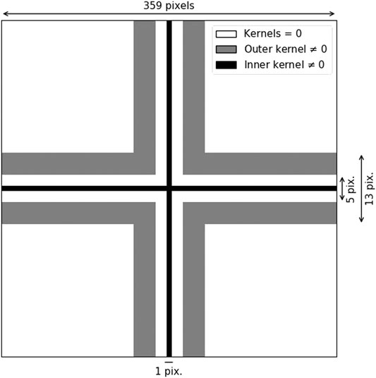
FIGURE 3. “Inner” and “Outer” kernels used for the reseau marker detection. Kernel values different from 0 are set such as the sum of all pixels is 1 (normalized).

3.1.2. Distortion Correction

The second preprocessing step is to correct for film and scanning distortion. The 2-D offset between the identified reseau markers and a 10 mm grid represents the distortion at each marker. It must then be interpolated at each pixel of the image. First, a polynomial transformation of degree 3 is removed to correct for the largest distortions of up to a few hundred pixels (primarily a rotation and scaling). The remaining distortion, usually a few pixels, can be very complex. As suggested by Maurer and Rupper (2015), we use a Thin-Plate Spline interpolation to estimate the distortion at every 100th pixel, and at full resolution using regular spline, due to memory limitations. The image is then re-sampled on the undistorted grid using a cubic spline interpolation.

3.1.3. Stitching and Cropping

The third preprocessing step is the image stitching and cropping. Because the image distortion can differ between scans, the two image halves are processed separately to generate distortion-free images. The two are then merged by first calculating an integer displacement between the overlap area of each image half using Normalized Cross-Correlation (NCC). The displacement is refined at sub-pixel accuracy by matching the position of the reseau markers, known with sub-pixel accuracy, between the two images. This showed better results than sub-pixel interpolation of the NCC results or matching of automatically identified interest points. The right part of the image is then re-sampled using bilinear interpolation and stitched to the left part. A final reseau markers’ detection is performed to check the quality of the distortion correction and stitching. Residual distortions are usually less than half a pixel. The reseau markers are then filled with Gaussian noise, whose mean and standard deviation are estimated from the neighboring pixels. We favored this approach over interpolation of the missing data (Surazakov and Aizen, 2010) to avoid introducing artifacts during the stereo processing, while reducing chances of matching between markers. Finally, the image is cropped to the approximate exposed area by removing pixels at a known distance from the outermost reseau markers. This ensures that all final images have the same dimensions (66,096 × 32,656 pixels) and principal point prior to stereo processing.

3.2. Stereo Processing

The stereo processing and DEM generation is performed using NASA’s open-source Ames Stereo Pipeline (ASP). The software abilities and workflow for processing Earth observation satellite data have been described extensively in Shean et al. (2016) and Beyer et al. (2018). Here we discuss the details of processing historical (frame camera) imagery with ASP.

ASPy iterative workflow consists of the following steps: camera initialization from crude image footprints, generation of inital DEMs, co-registration of the DEMs to a reference and update of the camera positions/orientations, refinement of the camera intrinsic parameters for each KH-9 MC, final DEM generation and DEM composite.

3.2.1. Camera Initialization

A pinhole camera model is initialized for each image by setting the camera intrinsic parameters to the documented values, i.e., focal length of 304.8 mm and principal point at the center of the reseau grid. An approximate camera position and orientation (extrinsic parameters) are estimated from the available footprint corner coordinates (assuming elevation of 0 m height above the WGS84 ellipsoid) using the ASP bundle_adjust tool. The corner coordinates have geolocation errors of several kilometers, so the resulting images will have inconsistent feature offsets, resulting in large stereo triangulation errors. To mitigate these issues, we perform a bundle adjustment optimization and iteratively refine camera extrinsic parameters (Beyer et al., 2018). Interest points are automatically identified for each image, matched between overlapping images and triangulated with available camera models to generate a sparse 3D point-cloud. The camera extrinsic parameters are then optimized to minimize the reprojection error, defined as the distance between the back-projected pixel location and true pixel location of each matched point.

3.2.2. Initial Digital Elevation Model Generation

We use the ASP pairwise stereo command to generate an initial DEM with the optimized camera models. First, the images of each stereo pair are aligned using an affine epipolar transformation to minimize the disparity between the two images. Second, a dense disparity (2D displacement between the left and right images) is calculated using the Smooth Semi-Global Matching algorithm (Facciolo et al., 2015), referred to as MGM in ASP or stereo-algorithm 2, with a 7 × 7 pixel correlation kernel. The algorithm has the advantage of using smaller windows than the more traditional NCC (stereo-algorithm 0, cost-mode 2 in ASP) and is therefore better at resolving sharp topographic features such as ridges or cliffs (see Section 4.4). The dense search is optimized for multi-processing and multi-threaded calculation. Each image is split in 5,000 × 5,000 pixel tiles and each tile is treated as an independent process to reduce total memory usage. For each tile, up to 8 threads are used to process 256 × 256 pixel blocks. To filter possible mismatches, the correlation is performed two ways, from left-image to right-image, then right-image to left-image. Areas where the two disparities differ, usually indicative of insufficient image texture, are discarded to remove spurious matches. This filter is later referred to as “xcorr filter.” While this option increases the computation time by a factor of about 2, we found it to be the most efficient way of removing outliers introduced by the MGM algorithm over featureless image areas (see Section 4.4). Stereo triangulation combines the disparity offsets and the camera models to produce a dense 3D point cloud in Earth-Center-Earth-Fixed (ECEF) coordinate system. The triangulation error is also computed to provide a confidence metric of the point-cloud. This is particularly useful to evaluate the camera models and the quality of the disparity matches. Finally, the point cloud is converted into a gridded DEM in a local projected coordinate system, using ASP’s point2dem tool, at a posting four times that of the input images (4 m × 6 m = 24 m² for native resolution of images scanned at 7 μm) that retains most of the topographic features present in the point-cloud while reducing DEM noise and artifacts (Shean et al., 2016). Note that ASP accounts for Earth curvature, which is critical due to the large extent of KH-9 MC images. To reduce computation time while providing a coarse DEM with sufficient posting (48 m) for the subsequent steps, we calculate this initial coarse DEM using images down-sampled by a factor of 2. The average run time for this stereo step with downsampled images was approximately 8 h on a dual 8-core 3.1 GHz Intel Xeon Sandy Bridge processor with 32 GB memory.

3.2.3. Digital Elevation Model Co-registration

This initial DEM can have geolocation errors of several kilometers and rotation/scaling errors due to uncertainties in the corner coordinates used to initialize the camera models. Traditional photogrammetric workflows involve manual identification of tie points and Ground Control Points (GCPs) to constrain the bundle adjustment and estimate precise camera extrinsic/intrinsic parameters. Unfortunately, this approach is manually intensive and does not scale for large numbers of images. Here, the KH-9 MC DEM is instead automatically co-registered to an external DEM using the ASP pc_align tool (see Section 2.4 for the list of reference DEM used in each region). The tool uses an Iterative Closest-Point (ICP) algorithm to estimate the transformation that minimizes offsets between the two point clouds (Beyer et al., 2018). As described in Section 2.5, glaciers and water bodies are masked in the reference DEM during these steps.

Rotation and scaling errors in the intial KH-9 MC DEMs can cause the standard ICP algorithm to fail, particularly when the DEM contains outliers. To overcome this, we use a two-stage co-registration approach. First, shaded relief maps are generated for both DEMs, match points between the two are identified, and a homography is calculated using RANSAC. This homography is applied to the KH-9 MC DEM, and a traditional ICP approach is used to estimate a final transformation. The transformation matrix is then used to update the camera extrinsic parameters. The refined camera models can then be used to generate DEMs and orthoimages with improved planimetric accuracy.

At this stage of the processing, residual elevation errors of several tens of meters are visible across the co-registered DEM when compared to the reference DEM (see Figures 4A,B). While some of this error is random, systematic biases persist due to unconstrained camera intrinsic parameters. For example, we observe a “bull’s-eye” pattern (Figure 4A) related to radial lens distortion, and biases correlated with the topography (Figure 4B) related to uncertainties in the camera focal length. These biases can be corrected by refining the camera intrinsic parameters (Figure 4D).

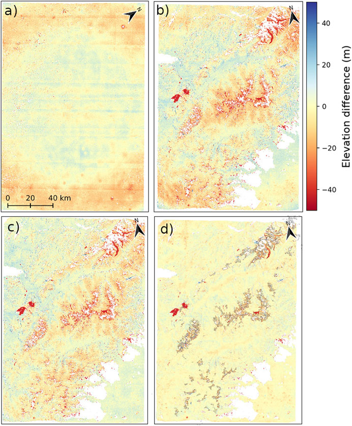
FIGURE 4. Examples of residual elevation biases in co-registered KH-9 MC DEMs before the refinement of camera intrinsic parameters. (A) “Bull’s eye” pattern caused by the lens distortion visible over flat terrain (pair DZB1212-500129-002/003) (B) Elevation biases correlated with topography over the central European Alps (pair DZB1216-500312-002/003). The high-elevation mountains appear higher than the reference DEM (red) whereas low-elevation valleys appear lower (blue). (C) Same as (B) but after lens distortion correction. (D) Same as (B) but after lens distortion and focal length correction. On this panel only, glaciers are outlined in black. North direction in each panel indicated by a black arrow.

3.2.4. Refining the KH-9 Mapping Camera Intrinsic Parameters

With the extrinsic parameters accurately known, a second bundle adjustment is performed to refine the camera intrinsic parameters, including the camera focal length and lens distortion. We use a Brown-Conrady lens distortion model, which represents the distortion for each pixel as a function of 8 parameters:

where ($x_d$, $y_d$) are the original distorted image pixel coordinates, ($x_u$, $y_u$) are the undistorted image pixel coordinates, ($x_c$, $y_c$) is the distortion center, $K_n$ is the nth radial coefficient and $P_n$ is the nth tangential coefficient and ϕ is the tangential distortion angle in radians.

The camera focal length, lens distortion parameters, and extrinsic parameters are simultaneously optimized using bundle adjustment for all available stereo pairs of a given KH-9 mission. For this step, a regular grid of several thousands match points is generated for each set of overlapping images (consecutive pairs or triplets) using the sub-pixel disparity maps. This ensures that the match points are equally distributed in the image and provide a strong constraint for the bundle adjustment. Additionally, the cost function minimized during this optimization is the sum of the reprojection error and the elevation error for all match points. The latter is calculated as the difference between the triangulated elevation at each of the matched interest points and the elevation sampled from the reference DEM. This bundle adjustment step results in a refined camera model (i.e., focal length and lens distortion) for each KH-9 mission.

3.2.5. Final Digital Elevation Model Generation

The mission-specific intrinsic parameters (Section 4.3) can then be used for other images from the same mission that were not used during optimization. However, the extrinsic parameters for these images must be updated. To accomplish this, we repeat the methodology in Sections 3.2.1 to 3.2.3.

The precise camera positions allow for the orthorectification of the full resolution images using the modern external DEMs with ASP mapproject tool. This step removes most of the terrain disparity signal, which both decreases the risk of mismatches and reduces computation time. However, residual offsets between the two orthorectified images exist where the reference terrain model is incorrect or surface elevation changed. A subsequent stereo step, following the same methodology as in Section 3.2.2, uses these residual feature offsets to generate a final DEM at 24 m posting. While a smaller posting is possible without oversampling, the larger pixel size means that more data points are averaged per pixel, which leads to more robust elevation estimates and fewer data gaps in the output DEM.

3.2.6. Composite Digital Elevation Model

Each overlapping stereo pair is processed to generate an independent DEM. Following bundle adjustment, all DEMs from overlapping images along the same orbit should be self-consistent. In practice, individual DEMs can have residual errors, especially DEMs from images with limited match points. To correct for this, each DEM is more precisely co-registered to a reference DEM (see Section 2.4) using the method outlined by Nuth and Kääb (2011). This approach usually outperforms the results obtained with ICP for horizontal shifts of less than a pixel. The KH-9 MC DEMs are then re-sampled to the reference DEM grid using a bilinear interpolation and the elevation difference is calculated. A 2D polynomial of degree two is estimated from the elevation difference over stable areas and removed from the map of elevation change. This can correct any residual large-scale distortion that may be caused by residual errors in the camera parameters. The magnitude of this correction is typically less than a few meters. All available DEMs are then merged into a single composite, taking the per-pixel average elevation value where there is overlap.

3.2.7. Evaluation of Stereo Processing Options

The quality of the final DEMs (vertical accuracy, coverage) is sensitive to the set of parameters used for stereo processing, in particular for the dense disparity map calculation. For this stage, several parameters must be chosen: the stereo matching algorithm, the correlation kernel size and the filtering options. ASP offers three options for the dense stereo matching algorithms, all of which attempt to find a match in the right image for each pixel in the left image (Beyer et al., 2018). The first is the standard NCC (–stereo-algorithm 0 –cost-mode 2) which extracts a “kernel” around each pixel in the left image, and searches for a corresponding match over a subset of the right image. The second is the Semi-Global-Matching (SGM) algorithm (Hirschmuller, 2008) which performs an NCC matching on smaller kernel sizes, but applies a smoothness constraint by minimizing a global cost function. The third is a smooth variant of SGM, called MGM, which reduces artifacts caused by SGM in low-texture areas (Facciolo et al., 2015) but is computationally more expensive.

We performed a series of systematic tests to evaluate correlation method, kernel size and filtering options. We tested NCC kernel sizes of 13, 17, 21. and 25 pixels, and SGM/MGM kernel sizes from 3 to 9 pixels (odd values only). The final results are also very sensitive to mismatches in areas with low image texture. To filter these outliers, two filtering options were tested: the xcorr filter and the standard deviation filter. The xcorr filter (“–xcorr-threshold 0” in ASP) was previously described in Section 3.2.2. The standard deviation filter, referred to as stddev, calculates the moving-window standard deviation in the input image and excludes pixels for which the standard deviation falls below a threshold. We calculated the standard deviation on windows of size 7 × 7 pixels, corresponding to the smallest template kernel used, and a standard deviation threshold of 3, or 0.01 for the normalized images used in ASP (–stddev-mask-kernel 7 –stddev-mask-thresh 0.01). Finally, for each combination of correlation and filtering parameters, we tested the impact of ASP stereo processing using original raw input images compared to input orthorectified images (Section 3.2.5).

We generated DEMs for each set of parameters using the same cloud-free KH-9 MC stereo pair over the Swiss Alps (DZB1216–500312L002/003), and used the “Hist 1980” reference DEM available for the same year for comparison (Section 2.4). For each output DEM, we computed total areal coverage and elevation difference statistics (median, 68% and 95% intervals, compared to reference DEM) for both stable and glacier surfaces. These metrics were used for a quality assessment, and to determine the parameter combination used for batch processing of the larger KH-9 MC archive.

3.3. Validation and Uncertainties

In this section, we estimate the uncertainty in the observed elevation changes at the pixel scale $\left({\sigma }_{dh}\right)$ and for spatially averaged elevation change $\left({\sigma }_{\text{Δ}h}\right)$.

3.3.1. Pixel-Scale Elevation Change Uncertainty

The elevation change uncertainty for each pixel, ${\sigma }_{dh}$, is estimated by the 68th and 95th percentiles (corresponding to 1 and 2 standard deviations for a normal distribution) of the distribution of absolute elevation differences. We determined statistics over both stable and glacierized surfaces. To do this, we computed elevation differences between the KH-9 MC DEMs and 1) overlapping, co-registered KH-9 MC DEMs along the same orbit or adjacent orbits with limited time offset, and 2) ancillary DEMs in the Alps and Alaska. Only historical DEMs acquired within one year of the KH-9 acquisitions (see Section 2.4) are used for the statistics over glacierized areas.

3.3.2. Spatially Averaged Elevation Change Uncertainty

3.3.2.1. Analytical Estimate

The uncertainty in the spatially averaged elevation change $\text{Δ}h$ (or volume change divided by area), is substantially reduced compared to the pixel-scale uncertainties by inter-compensation of random errors within the large averaging sample. For spatially independent (random) elevation change errors, the spatially averaged elevation change uncertainty is the standard error of the mean (SEM):

Where N is the number of pixels included in the average. However, it has been largely documented that for geodetic volume changes, there exist a spatial correlation between neighboring elevation change estimates that reduces N to an effective number of samples $N_{eff}$ (Nuth et al., 2007; Howat et al., 2008; Gardelle et al., 2012). Most of these studies make use of variograms in order to estimate the magnitude and range of this spatial correlation (Rolstad et al., 2009; Magnússon et al., 2016), but it is often unclear how the derived correlation range is used to calculate the number of independent observations (e.g., Howat et al., 2008; Berthier et al., 2010). Gardelle et al. (2012) suggested the following formulation:

where $PS$ is the pixel size and r the range of spatial correlation.

Alternatively, Rolstad et al. (2009) proposed an analytical approximation of ${\sigma }_{\text{Δ}h}$ based on spatial statistics. The uncertainty in the spatially averaged elevation change is derived by integration of a spherical variogram model on a circular region of radius L. Here, we reproduce their Eq. 11 for a spherical model with a zero nugget, a correlation range r and a sill s:

Note that the formula is valid both for distances below and above the spatial correlation range r, although in many cases, only the second term is used (Fischer et al., 2015; Shean et al., 2020) because most glaciers’ dimensions exceed the spatial correlation range typically estimated in these studies ($<$500 m). Additionally, this equation can be extended to any number of “nested” spherical models with varying ranges and sills, by summing the variances, to account for several ranges of spatial correlation (Appendix in Rolstad et al., 2009).

To constrain a nested spherical variogram model, we calculated elevation difference maps between 48 KH and –9 MC DEMs and the ArcticDEM. For each difference map, 2000 points were randomly extracted over stable terrain and used to calculate a variogram with lag distances ranging from 0 to 120 km (the swath width of a KH-9 MC image) using Python’s scikit-gstat library (Mälicke and Schneider, 2019). The variance was divided by the total variance of each difference map (i.e., standardized) to account for possible differences between DEMs. Several nested spherical models were then fit to the experimental variogram to estimate one or several correlation ranges and the associated sills. Finally, we used Eq. 4 to estimate the analytical uncertainty. The results were then compared to the SEM approach (Eqs 2and3) and an empirical estimate of the uncertainty.

3.3.2.2. Empirical Estimate

An empirical estimate of ${\sigma }_{\text{Δ}h}$ was obtained by calculating the standard deviation of average elevation changes for circular areas of increasing size over stable terrain (e.g., Miles et al., 2018). The average values are calculated by convoluting the elevation difference map with a normalized circular kernel of radius L, for L between 30 m and 120 km. The convolution accounts for gaps in the data and only average values with less than 10% data gaps were retained.

4. Results

4.1. Image Quality

The KH-9 MC image quality is excellent considering the age of the film. Visual inspection of the film copy at NARA revealed very finely resolved details, that are not fully captured by the scans. Some scratches and defects are visible, (Figure 2), but these artifacts are not coherent between images and therefore do not affect the stereo-processing used to generate the DEMs.

Despite the USGS’s high-quality scanning services, we identified several issues with scanned images that affected output DEM quality. Newton’s rings, interference patterns due to reflection between the scanner glass and the film, are sometimes visible in low contrast areas (Figure 2C). Small artifacts of up to a few millimeters were sometimes identified, with relatively consistent pixel location between successive images, and possibly related to dust grains or imprinted during film handling. They can represent a significant challenge for outlier rejection during the interest point matching, and lead to “pit” or “spike” artifacts in the final DEM (Figure 9D). Additionally, “tiling” artifacts are sometimes present in the final DEMs (Figure 9D; Supplementary Figure S5), due to systematic sub-pixel offsets in the scanned images, likely related to the Leica DSW700 scanner’s moving CCD sensor (see Section 5.1).

4.2. Preprocessing

ASPy’s automated preprocessing was successfully run on 698 images covering different types of landscapes from flat desert areas to high-relief Arctic regions (Section 2.3). The detection of the reseau grid is the most critical stage of the preprocessing as it is used to correct for image distortion and to merge the two scanned image halves. The raw distortion, estimated from the position of the reseau markers relative to a regular grid, usually consists of a rotation and scaling (Figure 5A), probably caused by a small misalignment of the film on the scanner and uncertainties in the scanner resolution. The average distortion for all images was about 200 pixels between opposite corners of the image half, or a total distortion of 0.4% for an image of $\sim$50,000 diagonal pixels. After correcting for an affine transformation (i.e. rotation and scaling), the median residual distortion was 0.8 pixels, with a maximum of 3.0 pixels (Figure 5B). Although small, the residual distortion displays a systematic pattern of shear along the margins of the film. In some cases a “gyre” pattern is visible, as previously reported by Surazakov and Aizen (2010) and Maurer and Rupper (2015). This shear pattern could be caused by the drive system during acquisition, film printing and/or duplication. No particular mention of this pattern was found in the declassified documentation, but it is recognized that the manipulation of the film can cause distortion and the reseau grid was implemented with the goal to correct for such distortion.

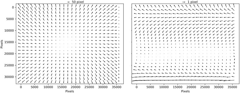
FIGURE 5. (A) Average image distortion for about 1400 KH-9 MC image halves, estimated from the observed position of the reseau markers relative to a regular grid. (B) Residual systematic distortion, after correcting for an affine transformation, showing systematic shear of the film.

4.3. Camera Intrinsic Parameters

Among the 698 preprocessed images, 424 were selected for the estimation of the camera intrinsic parameters (Section 2.3). The number of images available for each mission and the estimated camera intrinsic parameters are reported in Table 1.

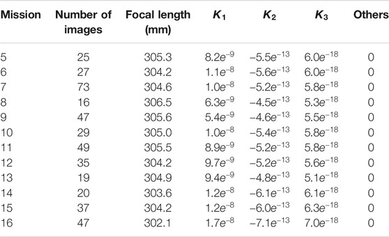
TABLE 1. Estimated camera intrinsic parameters for each of the twelve KH-9 mapping cameras.

The estimated focal length values showed significant deviation from the documented value of 304.8 mm or 12 inches (Burnett, 2012), ranging from 302.1 to 306.5 mm. Assuming a constant focal length value of 304.8 mm causes the distance between the satellite and the ground to be either over-estimated or under-estimated (Figure 4C). This issue resulted in systematic vertical DEM scaling errors, with residual elevation biases up to 15 m that were correlated with elevation (Figure 6C). By estimating a refined focal length for each mission, we reduced these errors to less than 5 m (Figure 6D).

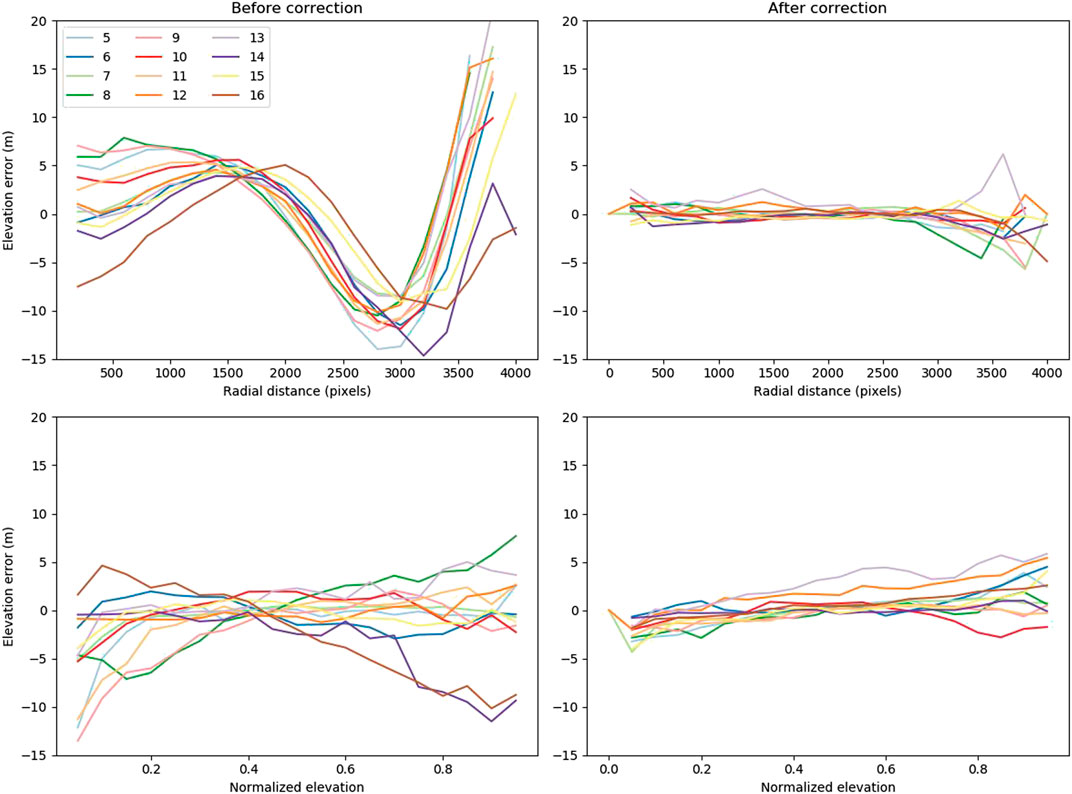
FIGURE 6. Average elevation bias of all KH-9 MC DEMs as a function of the distance to the DEM center (pixel size 30 m), for each of the twelve KH-9 missions equipped with MC (A) when lens radial distortion is neglected and (B) after correcting for lens radial distortion. Average elevation bias as a function of the normalized elevation $\left(\left[z-\text{min}\left(z\right)\right]/\left[\text{max}\left(z\right)-\text{min}\left(z\right)\right]\right)$(C) when assuming the documented focal length of 304.8 mm and (D) using the estimated focal length for each mission.

Our results indicate consistent lens radial distortion parameters between missions, with amplitudes varying slightly (parameters $K_1$–$K_3$ in Table 1). The maximum radial distortion associated with these parameters is about 50 μm ($\sim$7 pixels), which falls within the original requirements for the MC lens of less than 100 μm distortion (declassified document COS099307,³ Table 2.5). Neglecting the lens radial distortion results in relative elevation biases of $\pm$20 m in the individual KH-9 MC DEMs (Figure 6A). By estimating and correcting the lens distortion for each mission, we were able to reduce biases in the DEMs to less than 5 m (Figure 6B), with greatest residual error generally located for pixels furthest away from the image optical centers (image corners). These biases could possibly be corrected by higher order radial coefficients or with the use of more recently developed lens models (Wang et al., 2008). However such models are not yet available in ASP. All other parameters of the Brown-Conrady model had negligible values and did not show coherent sign or magnitude across the different missions. These parameters were therefore set to 0 for the rest of this study.

4.4. Stereo Processing Options

The details of the stereo processing analysis are included in the Supplementary Material. Here, we summarize the main findings.

We find that the ASP NCC correlator yields the most consistent results between the different set of options, with 95% error intervals systematically below 40 m (Supplementary Figure S1). The best results are obtained with a kernel size of 21 pixels and xcorr filter enabled (Figures 7A,B). Without this filter, blunders appear in areas of rugged topography and are likely related to the large kernel size that is unable to resolve small-scale features in the topography.

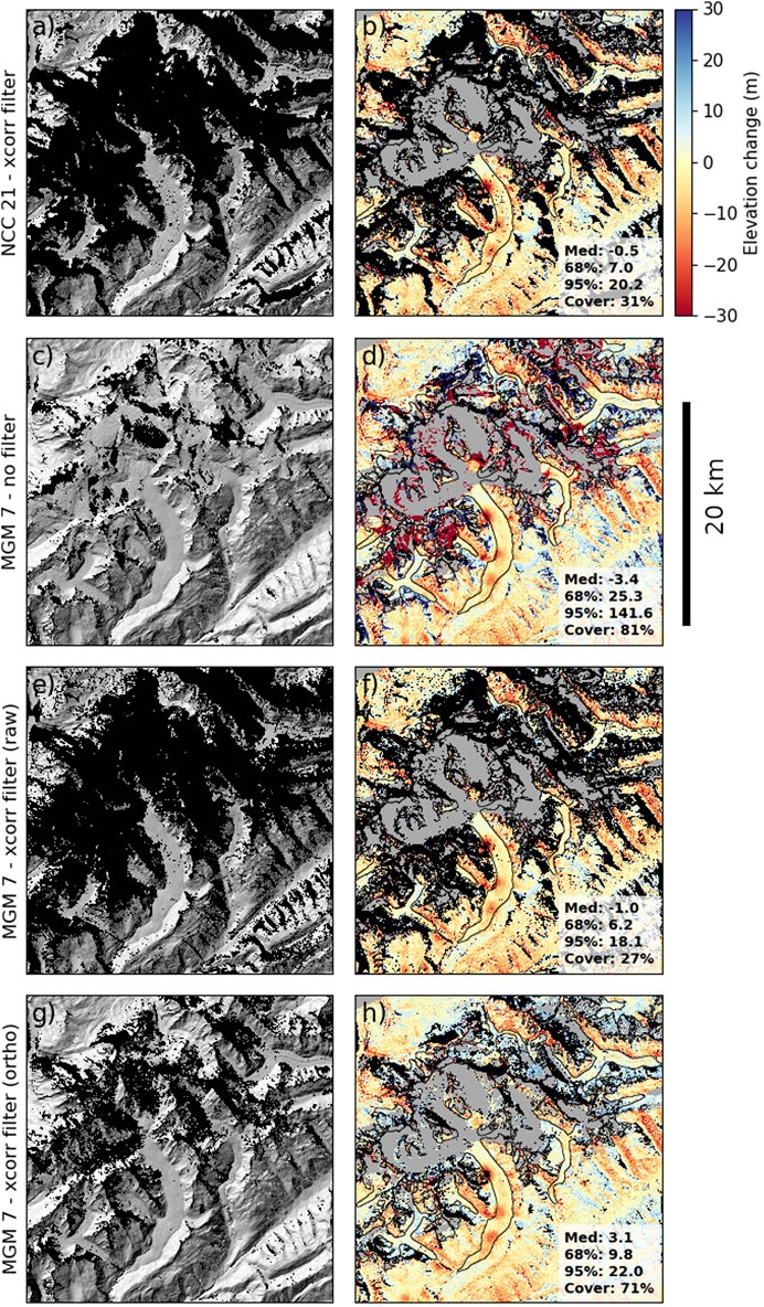
FIGURE 7. Elevation difference between KH-9 MC and “Hist 1980”” DEMs (right column) and shaded relief of the KH-9 MC DEMs (left column) over parts of the Swiss Alps for different ASP stereo processing options: (A,B) NCC with kernel size of 21 pixels and xcorr filter, (C,D) MGM with 7-pixel kernel and no filter, (E,F) same as (C,D) with xcorr filter, (G,H) same as (E,F) for orthorectified input images. Black areas represent gaps in KH-9 MC DEMs. In the right column, gray areas represent gaps in the “Hist 1980” DEM. Statistics of the elevation difference distribution [median (Med), 68 and 95 percentile and coverage (Cover)] are reported in each panel.

The ASP MGM correlator with xcorr filter produces DEMs with a slightly lower noise level and comparable coverage (Figures 7E,F). The best results are obtained with kernel sizes of 7–9 pixels (Supplementary Figure S1). In general, the outputs of MGM better represent small-scale surface features and display less random noise thanks to the use of smaller kernels and the smoothness constraint. However, this constraint can lead to remarkably large blunders in elevation. Errors in DEMs generated with SGM/MGM without any filtering can exceed 100 m, particularly for low-contrast surfaces as snow and ice (Supplementary Figure S1). This is because the SGM/MGM algorithms interpolates the disparity map in areas where no matches exist. In glacier accumulation zones, that are usually convex (U shaped), this often leads to an overestimate of the elevation, and an overestimate of the volume loss when the derived DEM is used for the earlier period (Figures 7C,D). Note that the SGM/MGM artifacts are only partially visible in the difference map (panel D) because of gaps in the aerial DEM, but are visible as a “crosshatched” pattern in the shaded relief (panel C). We were unable to filter these artifacts based on the image contrast as characterized by the stddev filter (Supplementary Figure S1). We therefore recommend always using the xcorr filter and increased quality control when using outputs from SGM/MGM. In general, the SGM algorithm does not perform as well as MGM, but conclusions regarding the choice of kernel size and filtering are similar.

Processing orthorectified images, rather than the raw images, leads to a significant increase in output DEM coverage (Supplementary Figure S2), i.e., fewer data gaps, especially in areas of low contrast or steep relief. This is consistent with the fact that orthorectification will reduce the parallax and hence decrease the chances of mismatches and blunders. In the case of MGM, using orthorectified input images leads to an increase in glacier coverage from $\sim$27 to 71% (Figures 7G,H), outperforming most NCC results (60% with a 21-pixel kernel). Elevation errors are slightly larger, likely related to the increased number of pixels sampled over challenging terrain. Note that the errors are again slightly reduced with MGM compared to NCC (Supplementary Figure S2).

We note that the use of the stddev filter with orthorectified images led to a negative elevation bias over glacier surfaces for our test case (median elevation change larger than 8 m in Supplementary Figure S2). Visual inspection of the results showed that the stddev filter creates a lot of small, isolated clusters of valid pixels surrounded by masked pixels in areas of low contrast. The interpolation by SGM/MGM of these likely erroneous values seem to have caused an overestimate of the elevation in these areas. We tested different sizes of stddev filters, from 7 to 35. Larger filters tend to remove these isolated clusters of pixels, but erode the mask around areas of low contrast, resulting in more blunders near margins of data gaps. Morphological operations (e.g., closing) on the stddev mask could help mitigate these issues, but we did not find a combination that outperformed the xcorr filter.

In summary, we found that unfiltered results can be strongly biased in low-texture areas and the xcorr filter was the most efficient at filtering those outliers. We therefore recommend using the ASP MGM correlation algorithm with xcorr filter enabled and a kernel size of 7 pixels (“stereo-algorithm 2 –corr-kernel 7 7 –xcorr-threshold 0”). Alternatively, NCC with 21-pixel kernel and xcorr filter (“–stereo-algorithm 0 –corr-kernel 21 21 –subpixel-kernel 21 21 –subpixel-mode 3 –xcorr-threshold 0”) offers a good alternative, especially for “raw” input images, with up to a five-fold reduction in processing time. Additionally, the spatial coverage is significantly improved when first orthorectifying the KH-9 images with a reference DEM, but requires that the camera position is well estimated prior to the orthorectification.

4.5. Validation and Uncertainty

4.5.1. Pixel-Scale Elevation Change Uncertainty

The distribution of absolute elevation differences for overlapping KH-9 MC DEMs is shown in Figures 8A,B for the Alps and Alaska. The KH-9 MC elevations are self-consistent with a vertical precision of about 5 m (68% confidence level) and 15 m (95%). Most importantly, the DEM uncertainty is similar for pixels located on and off glacier surfaces, indicating effective filtering of DEM outliers over low-texture snow and ice surfaces.

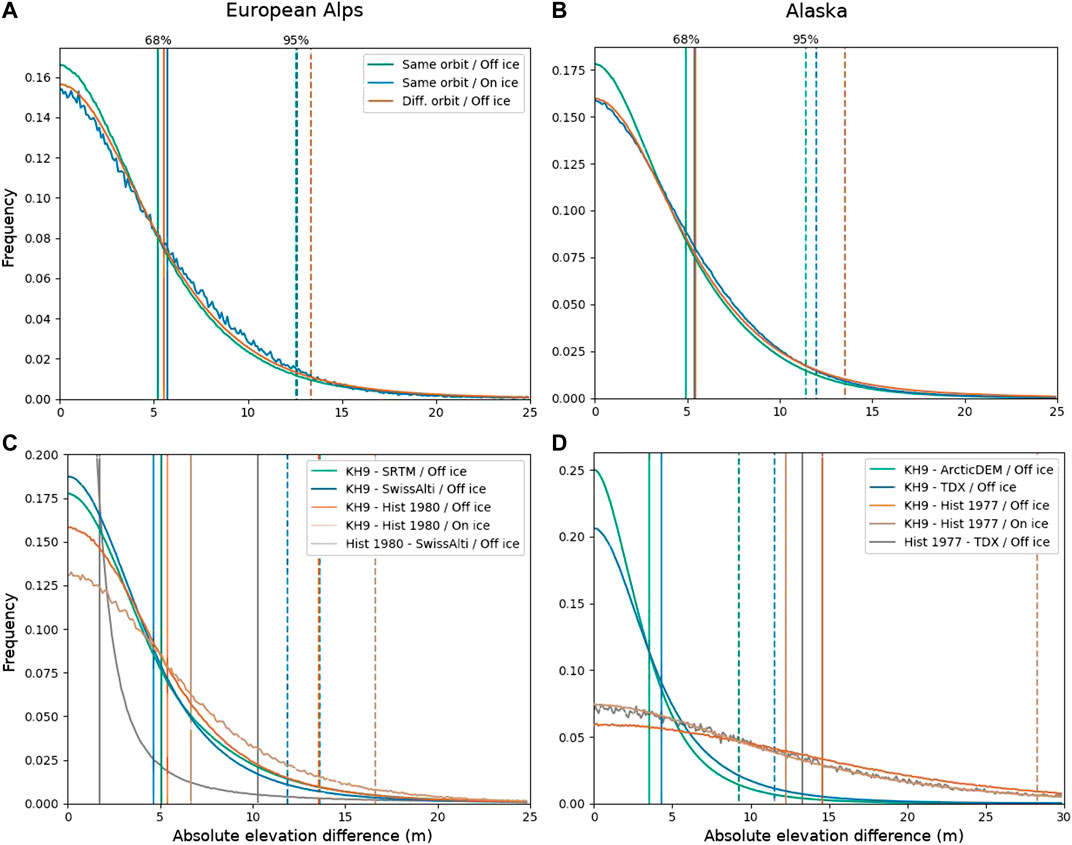
FIGURE 8. Distributions of absolute elevation differences for KH-9 MC DEMs over the Alps (left column, 8 DEMs) and Alaska (right column, 48 DEMs). The top row (A,B) shows the elevation difference between overlapping KH-9 MC DEMs from the same orbit (same date) or different orbits. The bottom row (C,D) shows the elevation difference between the KH-9 MC DEMs and several ancillary DEMs. Solid and dashed vertical lines indicate the 68th and 95th percentiles of the distributions, respectively.

The distributions of absolute elevation difference values between the KH-9 MC DEMs and reference ancillary DEMs are shown in Figures 8C,D. The estimated uncertainty is similar to the MC cross-comparison: $\sim$5 m at 68% and less than 15 m at 95% for most ancillary DEM sources. The comparison with historical DEMs acquired within the same year as the KH-9 MC DEMs enables us to estimate the uncertainty on glacier surfaces. A slightly larger on-ice uncertainty is obtained for the Alps pair (“Hist 1980”) compared to off-ice uncertainty. However, the Alaska results (“Hist 1977”) show much larger uncertainty both on and off-ice. This difference can be largely explained by the larger uncertainty of the “Hist 1977” DEM, as is demonstrated by the larger residuals off-ice when compared with the TanDEM-X DEM (gray lines). These results highlight the benefit of the KH-9 MC DEMs compared to digitized historical topographic maps. For the rest of our analysis, we use a value of ${\sigma }_{dh}$ = 5 m (68% interval) for per-pixel DEM uncertainty. In the next section, we discuss scaling of this ${\sigma }_{dh}$ when averaging over variable area.

4.5.2. Spatially Averaged Elevation Change Uncertainty

The pixel-scale uncertainty, however, does not reveal potentially spatially correlated errors that would accumulate when deriving a volume change. Visual inspection of the elevation change maps shows that such correlated errors exist with several spatial scales (Figure 9D). This correlation can be quantitatively assessed using variograms.

FIGURE 9. Spatial correlation of DEM error in the KH-9 MC DEMs and scaling for area averaging. Observed (gray dots) and modeled (lines) variograms for elevation differences between 48 KH-9 MC DEMs and ArcticDEM mosaic over Alaska for (A) short lag distances ($<$6 km) and (B) all lag distances. The best fit variogram model (orange dashed lines) is the sum of three nested spherical models (green, blue and yellow lines). (C) Empirical standard error of the mean (SEM) as a function of the averaging area for all 48 DEM differences (gray lines) and the median values (black line) compared to several analytical estimates (R09 refers to Rolstad et al. (2009) model for corresponding range r) and our best-fit triple-nested variogram model (orange dashed line). (D) Sample elevation difference map for KH-9 MC pair DZB1212-500129002/003 (essentially ice-free area), with typical artifact length scales noted.

The empirical variogram obtained from the KH-9 MC and ArcticDEM elevation difference maps over Alaska is shown in Figure 9A,B. Fitting a single spherical model to the variogram did not provide satisfying results because of the substantial increase in variance for large lag distances. Using a sum of 2 (not shown) and 3 spherical models improved the fit, while higher order models did not provide significant improvements. We find that spatial correlation ranges of 462, 4,758 and 65,631 m explain about 46, 34, and 20% of the variance, respectively (Figure 9B). The shortest correlation range is in line with previous estimates for KH-9 MC DEMs (Pieczonka et al., 2013; Maurer et al., 2016; Goerlich et al., 2017; Zhou et al., 2018). However, this short-range correlation alone explains less than half of the total elevation error variance. These short-range errors become negligible when averaging over the typical range of glacier areas (2 km², dashed green line in Figure 9C). The longer correlation ranges of several to tens of kilometers dominate the total area-averaged uncertainty, and it is essential to reliably assess their contribution to spatially averaged elevation change uncertainty. These different correlation ranges captured by our spatial variograms are compatible with patterns visible in individual elevation change maps (Figure 9D): short-scale ($\sim$500 m) random noise likely due to film grain and correlation error, $\sim$3–4 km scale artifacts likely caused by residual image distortion (3–4 km), and $\sim$70 k $>$ m artifacts related to scanner tiling issue.

Following the method described in Section 3.3.2.2, we estimated an empirical uncertainty in the spatially averaged elevation change from the same elevation difference maps. The result is shown in Figure 9C (gray and black lines), along with the analytical estimate from Eq. 4 for a single spherical model of range 500 m (green curve) and 70 km (yellow curve). The estimate obtained using Eqs 2and3 with a 500 m range is also shown (dashed blue curve). All results are represented as a function of the equivalent circular area $\left(\pi L^2\right)$. Our empirical uncertainty decreases with increasing averaging area, but values are much larger than would be estimated using only a short-range correlation of 500 m (blue and green curves). Moreover, for distances below the 500 m correlation range, Eq. 2 is not valid and overestimates the uncertainty. The Rolstad et al. (2009) model (Eq. 4) with single correlation range of 500 m (green curve) shows better agreement with the empirical uncertainty for smaller averaging areas, but also underestimates the uncertainty for larger averaging areas. If we instead use a single correlation range of 70 km, we obtain a conservative estimate of the uncertainty (yellow curve). A better estimate of the uncertainty can be obtained using the correlation ranges estimated from the variogram (orange curve). By summing Eq. 4 for three correlation ranges ($r_1$ = 0.5 km, $s_1$ = 0.46, $r_2$ = 5.0 km, $s_2$ = 0.34, $r_3$ = 70.0 km, $s_3$ = 0.20), we are able to closely reproduce the empirical uncertainty. The agreement between empirical and analytical approaches gives us confidence in our three spherical model for estimating uncertainty in spatially averaged elevation change (Rolstad et al., 2009).

4.5.3. Geodetic Glacier Volume Change

In this section, we estimate glacier geodetic volume change and associated uncertainty from KH-9 MC DEMs over an 820 km glacierized area in Southwest Switzerland (see Section 2.4). A composite DEM was calculated by taking the average value from two KH-9 MC image pairs available over the Alps in September 1980 (strip DZB1216–500312, images 2 to 4). We then computed the elevation difference between the modern 2018 SwissAlti3D DEM and both the historical aerial DEM “Hist 1980” (Figure 10A) and the KH-9 MC DEM composite (Figure 10B). The two historical DEMs cover 57 and 56% of the glaciers in the region, respectively. Gaps in the historical DEMs are prevalent for higher elevations due to the lack of surface texture over snow and saturation of the aerial/satellite film over highly reflective snow and ice surfaces. Note that by combining DEMs obtained from all available KH-9 MC image pairs over the study area (8 over a five year period), the glacier coverage increases to 85%.

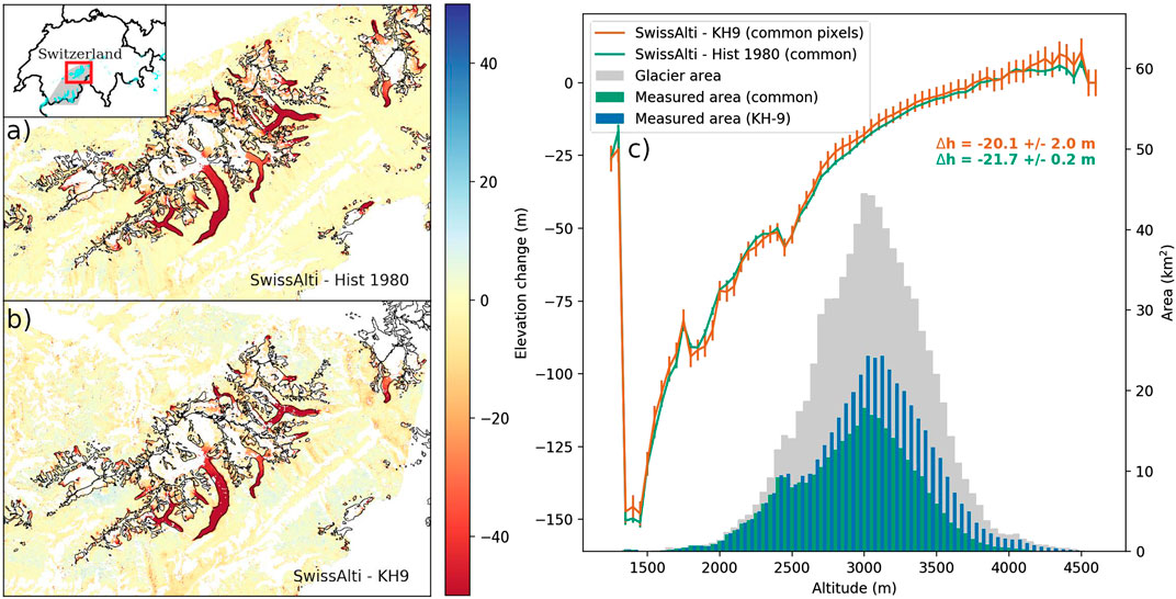
FIGURE 10. Detail of elevation change maps on a subset of Swiss glaciers obtained by comparing the 2018 DEM SwissAlti3D with (A) the historical 1980 aerial DEM and (B) a 1980 KH-9 MC DEM composite, with black glacier outlines. Inset shows the location map for the whole area analyzed, corresponding to the 1980 aerial DEM extent (gray), zoom extent (red) and glaciers (light blue). (C) Elevation change as a function of altitude from the 1980 aerial DEM (green line) and KH-9 MC DEMs (orange line) with 1−σ error bars for each 50 m bin. The histograms show the hypsometric distribution of glacier area (gray), area common to both historical DEMs (green) and area from KH-9 MC DEM alone (blue).

To account for elevation data gaps, the region-wide glacier elevation change is estimated by multiplying the median elevation change in 50 m altitude bins by the glacier area in that bin, following the regional hypsometric method (McNabb et al., 2019). We also considered the bin mean to test the sensitivity of our statistical approach. For the comparison, the median values are calculated solely for the pixels common to both historical DEMs. Finally, the uncertainty in elevation change for each altitude band is estimated following the methodology described in Section 4.5.2, both for the KH-9 MC and the aerial DEMs (see Supplementary Figure S3 for the aerial DEM). Figure 10C shows the resulting elevation change vs elevation profiles and hypsometry for all glaciers in the study region. The KH-9 MC DEM elevation change profile is very similar to the profile from the historical aerial DEM (our “truth”). This demonstrates that the KH-9 MC elevations are not biased on glacier surfaces at any altitude. The region-wide median (mean) glacier elevation change over the approximately 38-year period estimated with the KH-9 MC DEM composite is –20.1 $\pm$ 2.0 m (–21.3 m), as compared to –21.7 $\pm$ 0.2 m (–22.4 m) for the historical aerial DEM. Both estimates overlap at the 1–σ (68%) confidence level. Note that the error bars only reflect uncertainties in the elevation difference, and do not include uncertainties associated with data gaps or glacier area (McNabb et al., 2019; Shean et al., 2020), that are not the focus of this study.

5. Discussion

5.1. Image Distortion and Scanning Artifacts

We show that distortions of over 100 pixels (at 7 μm resolution) are common on the digitized declassified imagery provided by the USGS, scanned with state-of-the-art photogrammetric scanners. Holzer et al. (2015) reported similar image distortion, while Surazakov and Aizen (2010) and Maurer and Rupper (2015) reported smaller amplitudes of a few pixels only, similar to the residual distortion we obtained after correcting for rotation and scaling. Such image distortion must be corrected prior to any quantitative use of the scanned images requiring sub-pixel precision (i.e., DEM generation). The largest distortion is a rotation and possibly scaling of the scanned images, and can be corrected with a minimum of three fiducial markers, available on most historical data. The KH-9 MC images include 1,081 fiducial markers that enables correcting for image distortions of a few tens of microns, likely introduced during film handling and storage. The impact of such distortion will depend on the pixel resolution. In the case of the KH-9 MC, this can lead to elevation biases of several meters, but this impact will be smaller for higher resolution analog imagery.

Additionally, our results revealed “tiling” artifacts in the scanned images that translate into a rectangular pattern of elevation offsets in the DEMs (Figure 9D; Supplementary Figure S5). These artifacts are likely caused by the Leica DSW700 scanner, which captures portions of the film with a moving CCD sensor with dimensions of 4,000 × 2,700 pixels (Gheyle et al., 2011). The artifacts could be introduced during the mosaicking of the final image. Two arguments lean toward this conclusion. First, the scanner CCD sensor size corresponds to the size of the tiling pattern visible on the elevation change maps (two patterns from each image of the stereo pair are superimposed). Second, these artifacts are also visible as a slight change in image intensity values between tiles, as revealed by applying a standard deviation filter on the original scanned images before any preprocessing (Supplementary Figure S4). This confirms that the artifacts were not introduced during our processing. Similar issues resulting in artifacts of larger amplitude were previously identified and fixed for this scanner (Gheyle et al., 2011).

We participated in several exchanges with the USGS to identify the causes of these scanning artifacts. Unfortunately, the issue could not be traced to a specific scanner or scanning period. The scanning artifact issue remains unresolved, and likely affects a significant portion of the previously scanned images in the EarthExplorer archive. Since the position and amplitude of these artifacts in the scanned images is variable, it is challenging to develop custom corrections. A possible solution would be to correct the elevation in the final DEMs assuming sufficient stable terrain is available, but the superimposition of two patterns makes the problem challenging and would require tracking a pixel from the raw image all the way to the final DEM, through the different preprocessing and stereo processing steps.

5.2. Camera Calibration

We developed a methodology to accurately estimate camera extrinsic and intrinsic parameters for the KH-9 MC, without the use of manually identified GCPs. This methodology relies on approximate image geolocation and the availability of a reference DEM with a posting similar to, or better than, the output DEMs. It is similar to the methodology proposed by Maurer and Rupper (2015) with the main difference that in their methodology, the camera intrinsic parameters are estimated for each stereo pair based on the tie points only. Our approach optimizes a single set of intrinsic parameters for each satellite mission and uses the reference DEM as an additional constraint during bundle adjustment. Since the intrinsic parameters are estimated for each mission, they can more easily be transferred to other images from the same mission for which the surface conditions or exposure prevent camera parameter estimation. A question arises as to whether the camera intrinsic parameters can be assumed constant for the duration of a mission. Changes in instrument temperature during an orbit or spacecraft vibrations could cause slight changes in these parameters. To test this we estimated intrinsic parameters for individual stereo pairs or consecutive tracks following the same approach used for the full mission. The estimated camera parameters showed some variability but the differences were equally large for images acquired at a few minutes or several weeks interval. Because of this, we attributed the variability in image-pair parameters to the uncertainty of the retrieval method and differences in image quality or scene characteristics, and not to real changes in camera parameters. Pre-flight and on-orbit KH-9 MC camera calibration was performed with 2 μm required accuracy (Burnett, 2012) but the detailed calibration data are not presently available, either still classified or not archived. The release of such information in the future would help to validate our results and improve the quality of the KH-9 MC DEMs.

5.3. Application to Other Historical Image Sources

We further discuss the applicability of the method to other historical data sets such as historical aerial images (Vargo et al., 2017; Girod et al., 2018) or other declassified data (Galiatsatos et al., 2007; Fowler, 2013). The method consists in three main steps: 1) Initialize cameras with approximate geolocation and focal length 2) Co-register the initial DEM with reference terrain model 3) Optimize the camera intrinsic and extrinsic parameters that minimize output DEM offsets relative to the reference elevation data.

The first step requires image geolocation information. The KH-9 MC images and other declassified images provided by the USGS have approximate corner coordinates, often with tens of kilometers of error. This step also requires knowledge of an approximate focal length. Without any prior information, the focal length can be assumed to be similar to the image size. If no geolocation information is available, the automatic identification of tie points between the historical imagery and ancillary imagery with good geolocation information (e.g., Vargo et al., 2017) could offer an alternative, though this approach can be challenging for evolving landscapes or oblique images (Girod et al., 2018).

The second step is to co-register the initial DEM with a reliable reference. Because topographic features remain much more stable than surface radiance (e.g., seasonal snowcover), finding matches between historical and a reference terrain is much easier than finding matches between two images acquired at different times, with different orientation and posting (Girod et al., 2018). The two DEMs can first be roughly co-registered with a homography using standard feature detection and matching (e.g., SIFT) and an outlier rejection (e.g., RANSAC). The co-registration can then be refined using ICP. The obtained transformation matrix can then be applied to the camera extrinsic matrices to obtain the updated camera positions. To improve success it is recommended to use DEMs with similar posting and with as much stable terrain as possible.

The third step involves generating a sufficiently large and well-distributed sample of GCPs over stable ground to constrain the bundle adjustment for the camera intrinsic refinement. After the output DEM is co-registered to a reference, GCPs can be generated by extracting points from the disparity map and calculating the ground coordinates of these pixels. The “true” elevation of these coordinates can then be sampled from the reference DEM, and the residual elevation difference on stable terrain can be used to refine the intrinsic parameters. The last two steps can be iterated if the initial lens distortion is too large to ensure successful co-registration of the intermediate DEMs.

5.4. Uncertainty in Elevation Changes

We find a 68% confidence interval in KH-9 MC DEM pixel elevations of about 5 m, and less than 15 m at the 95% level, when processed with ASPy. A 5 m uncertainty is equivalent to about one pixel (or 7 microns) in the original images, which is typically the accuracy that can be achieved in the best conditions in a photogrammetric processing. This is an improvement of 2–3 times over previous results obtained from workflows involving manually selected GCPs (Pieczonka et al., 2013; Holzer et al., 2015; Zhou et al., 2018) and similar to other automated workflows (Maurer and Rupper, 2015; Maurer et al., 2019), although some of the earlier studies may have been based on 14 μm resolution scans (Pieczonka et al., 2013, e.g.). We note that our uncertainty estimates are rather conservative as they cover a large variety of images, terrain and do not exclude steep slopes that are prone to larger errors. The estimates also incorporate uncertainties inherent to our reference DEMs used to calculate the elevation difference. The fact that the 68th and 95th percentiles were similar for all reference DEMs (except for “Hist 1977”) suggests that the KH-9 MC DEMs dominate the elevation change uncertainty. Additionally, we demonstrated that uncertainties do not increase for snow and ice-covered terrain.

A direct consequence of the scanning issues mentioned above is that the output DEMs show correlated biases over large distances. The variogram analysis showed that correlation ranges of 500 m typically used by other studies (Pieczonka et al., 2013; Maurer and Rupper, 2015; King et al., 2019) account for only 50% of error variance and about 20% of this variance is explained over distances of several tens of kilometers. These results have several implications for the estimation of uncertainties in spatially averaged elevation data derived from stereo imagery. First, if large-scale correlated instrument errors can be discriminated visually on elevation difference maps, then it is unlikely that the spatial correlation can be represented by a single spherical model as is done in most surface deformation studies. Empirical and analytical approaches exist to estimate spatial correlation and spatially integrate correlated data, and should be used together to cross-validate assumptions regarding uncertainty propagation. When sampling an empirical variogram, we recommend to 1) calculate the variance for spatial lags up to about half the longest image dimension to identify potentially long correlation ranges and 2) use the standardized variance (i.e., divided by the total variance). The latter is expected to converge toward 1 for very long spatial lags, which helps to ensure that the variograms are calculated over sufficient long lags. In the case of KH-9 MC images, we found three correlation ranges of approximately 0.5, 5, and 70 km. Using a single correlation range of 500 m would result in an underestimation of the uncertainty by a factor 4 over an averaging area of 10 km², a factor of 9 over 100 km², and 33 over 100,000 km². Second, we recommend using the full Eq. 4 and not only the formula valid for distances larger than the spatial correlation range (second line in the equation). In case of large correlation ranges, this formula would be invalid for most areas considered.

Finally, Eq. 3 has been used repeatedly to estimate the uncertainty of spatially averaged elevation changes (Gardelle et al., 2013; Wang and Kääb, 2015; Berthier et al., 2016; Bolch et al., 2017; Zhou et al., 2018; King et al., 2019). This formulation was derived for a one-dimensional case (Bretherton et al., 1999; Eq. 1), and is invalid for a 2-dimensional case. As demonstrated in Rolstad et al. (2009) and reproduced in Eq. 4, the spatially averaged elevation change uncertainty should be directly proportional to the correlation range r, rather than to the square root. The erroneous application of this formula tends to underestimate the uncertainty for long ranges. Therefore, the rigorous integration approximation proposed by Rolstad et al. (2009) that is based on spatial statistics, and implemented here for multiple spatial correlations, should be used instead.

6. Conclusions

Despite many processing challenges, the value of historical airborne or satellite stereo imagery in the geosciences has long been recognized. Over the past decade, several studies used traditional and modern photogrammetry approaches to derive DEMs from these data. In this paper, we presented ASPy, an automated workflow to generate DEMs from analog Hexagon (KH-9) mapping camera images, which covered nearly all of Earth’s land surface between 1973 and 1980. ASPy is able to convert the raw scanned images into distortion-free images by identifying the sub-pixel location of all 1,081 markers present on the images. Stereo pairs are then processed using the Ames Stereo Pipeline to generate DEMs with 24 m posting. The processing uses the crude image geolocation provided by the USGS and an external DEM to avoid the labor-intensive process of manually identifying GCPs. We processed 424 images to estimate camera intrinsic parameters (focal length and lens distortion) for each of the twelve missions of the KH-9 program with MC instruments, thereby correcting systematic errors of several tens of meters in the output DEMs. These camera parameters can be used in the future to process KH-9 MC images in challenging terrain, such as in the polar regions, where the lack of stable terrains would prevent a camera calibration. The KH-9 derived DEMs were validated against modern DEMs over stable terrain, and ancillary historical DEMs with similar acquisition dates over snow and ice covered terrain in Switzerland and Alaska. The pixel-scale elevation uncertainty was estimated as $\sim$5 m at 68% confidence level, and less than 15 m at 95% level. We evaluated the uncertainty of spatially averaged elevation change both from an empirical and analytical approach, and find consistent agreement. We raise particular attention to large-scale correlated biases in elevation associated with such analog imagery that must be taken into account to derive statistically significant elevation and volume change estimates. However, our results show that with care, the KH-9 MC archive represents a suitable dataset for global scale, long-term elevation change studies with potential applications in glaciology, seismology, natural hazards, hydrology or geomorphology.

Data Availability Statement

The KH-9 MC images are freely available from the USGS. The KH-9 MC DEMs produced as part of this study will be released in a follow-up glacier change analysis and can be made available upon request to the corresponding author.

Author Contributions

AG and AD designed the study. AD developed the workflow, processed the data, and conducted the analysis with inputs from AG, OA, SM, and DS. OA and SM implemented modifications to ASP required for the KH-9 MC data. RH provided input on the uncertainty analysis. MM processed and provided the Swiss historical aerial DEM. AD led the writing of the paper and all co-authors contributed to it.

Funding

AG and AD were funded by the NASA’s Cryospheric Sciences and MEaSUReS Programs through award to AG. The research was conducted at the Jet Propulsion Laboratory, California Institute of Technology, under contract with the National Aeronautics and Space Administration. AD acknowledges funding from the Swiss National Science Foundation, grant no. 184634. DS was supported by a University of Washington Innovation Award.

Conflict of Interest

The authors declare that the research was conducted in the absence of any commercial or financial relationships that could be construed as a potential conflict of interest.

Acknowledgments

We thank Etienne Berthier for sharing the historical Alaska DEM, Mike Willis for his help with the ancillary DEMs and Antoine Rabatel for sharing (unused) data set over the French Alps. We would like to thank Tobias Bolch for valuable feedback on a first round of reviews. We thank the JPL super-computing facilities and in particular Edward Villanueva for his technical support. This work would not have been possible without the open access to the KH-9 MC images and the outstanding work of the USGS to make this data accessible to everyone. We are particularly grateful to Tim Smith and Ryan Longhenry for the exchanges regarding the scanning issues. We acknowledge open access data provided by the Polar Geospatial Center (ArcticDEM), the DLR (TanDEM-X 90 m DEM) and NASA (SRTM). The swissAlti3D DEM was purchased from the Swiss Federal Office of Topography, license no. JD100042.

Supplementary Material

The Supplementary Material for this article can be found online at: https://www.frontiersin.org/articles/10.3389/feart.2020.566802/full#supplementary-material

Footnotes

¹ https://www.nro.gov/Portals/65/documents/foia/declass/ForAll/101917/F-2017-00094c.pdf - last accessed April 10, 2020.

² © 2020 swisstopo - Available online at https://shop.swisstopo.admin.ch/en/products/height_models/alti3D (Last accessed on August 25, 2020).

³ https://www.nro.gov/Portals/65/documents/foia/docs/HOSR/SC-2017-00006l.pdf (last accessed on April 09, 2020).

References

Anderson, S. W. (2019). Uncertainty in quantitative analyses of topographic change: error propagation and the role of thresholding. Earth Surf. Process. Landforms 44, 1015–1033. doi:10.1002/esp.4551
Belart, J. M. C., Magnússon, E., Berthier, E., Pálsson, F., Adalgeirsdóttir, G., and Jóhannesson, T. (2019). The geodetic mass balance of Eyjafjallajökull ice cap for 1945-2014: processing guidelines and relation to climate. J. Glaciol. 65, 395–409. doi:10.1017/jog.2019.16
Berthier, E., Cabot, V., Vincent, C., and Six, D. (2016). Decadal region-wide and glacier-wide mass balances derived from multi-temporal ASTER satellite digital elevation models. Validation over the Mont-Blanc area. Front. Earth Sci. 4, 63. doi:10.3389/feart.2016.00063
Berthier, E., Schiefer, E., Clarke, G. K. C., Menounos, B., and Rémy, F. (2010). Contribution of Alaskan glaciers to sea-level rise derived from satellite imagery. Nat. Geosci. 3, 92–95. doi:10.1038/ngeo737
Beyer, R. A., Alexandrov, O., and McMichael, S. (2018). The Ames stereo pipeline: NASA’s open source software for deriving and processing terrain data. Earth Space Sci. 5, 537–548. doi:10.1029/2018EA000409
Bhambri, R., Bolch, T., and Chaujar, R. K. (2012). Frontal recession of Gangotri Glacier, Garhwal Himalayas, from 1965 to 2006, measured through highresolution remote sensing data. Curr. Sci. 102, 489–494. doi:10.5167/uzh-59630
Bhambri, R., Bolch, T., Kawishwar, P., Dobhal, D. P., Srivastava, D., and Pratap, B. (2013). Heterogeneity in glacier response in the upper Shyok valley, northeast Karakoram. Cryosphere 7, 1385–1398. doi:10.5194/tc-7-1385-2013
Bolch, T., Pieczonka, T., Mukherjee, K., and Shea, J. (2017). Brief communication: glaciers in the Hunza catchment (Karakoram) have been nearly in balance since the 1970s. Cryosphere 11, 531–539. doi:10.5194/tc-11-531-2017
Bolch, T., Yao, T., Kang, S., Buchroithner, M. F., Scherer, D., Maussion, F., et al. (2010). A glacier inventory for the western Nyainqentanglha range and the Nam Co Basin, Tibet, and glacier changes 1976–2009. Cryosphere 4, 419–433. doi:10.5194/tc-4-419-2010
Bretherton, C. S., Widmann, M., Dymnikov, V. P., Wallace, J. M., and Bladé, I. (1999). The effective number of spatial degrees of freedom of a time-varying field. J. Clim. 12, 1990–2009. doi:10.1175/1520-0442(1999)012%3C1990:TENOSD%3E2.0.CO;2
Burnett, M. (2012). Hexagon (KH-9) mapping camera Program and evolution (national reconnaissance Office (NRO)). Chantilly, VA: Center for the Study of National Reconnaissance (CSNR).
Facciolo, G., Franchis, C. D., and Meinhardt, E. (2015). “MGM: a significantly more global matching for stereovision,” in Proceedings of the British Machine Vision Conference (BMVC), September 2005, Available at: .
https://dx.doi.org/10.5244/C.29.90CrossRef Full Text | Google Scholar
Farr, T. G., Rosen, P. A., Caro, E., Crippen, R., Duren, R., Hensley, S., et al. (2007). The shuttle radar topography mission. Rev. Geophys. 45, RG2004. doi:10.1029/2005RG000183
Feranec, J., Soukup, T., Hazeu, G., and Jaffrain, G. (2016). European landscape dynamics: CORINE land cover data. Boca Raton, FL: CRC Press, 368.
Fischer, M., Huss, M., and Hoelzle, M. (2015). Surface elevation and mass changes of all Swiss glaciers 1980–2010. Cryosphere 9, 525–540. doi:10.5194/tc-9-525-2015
Fischler, M. A., and Bolles, R. C. (1981). Random sample consensus: a paradigm for model fitting with applications to image analysis and automated cartography. Commun. ACM 24, 381–395. doi:10.1145/358669.358692
Fowler, M. J. (2004). Archaeology through the keyhole: the serendipity effect of aerial reconnaissance revisited. Interdiscipl. Sci. Rev. 29, 118–134. doi:10.1179/030801804225012635
Fowler, M. J. F. (2013). “Declassified intelligence satellite photographs,” in Archaeology from historical aerial and satellite archives. Editors W. S. Hanson, and I. A. Oltean, (New York, NY: Springer New York), 47–66.
Fujita, K., Takeuchi, N., Nikitin, S. A., Surazakov, A. B., Okamoto, S., Aizen, V. B., et al. (2011). Favorable climatic regime for maintaining the present-day geometry of the Gregoriev Glacier, Inner Tien Shan. Cryosphere 5, 539–549. doi:10.5194/tc-5-539-2011
Galiatsatos, N., Donoghue, D. N., and Philip, G. (2007). High resolution elevation data derived from stereoscopic CORONA imagery with minimal ground control. Photogramm. Eng. Rem. Sens. 73, 1093–1106. doi:10.14358/PERS.74.9.1093
Gardelle, J., Berthier, E., Arnaud, Y., and Kääb, A. (2013). Region-wide glacier mass balances over the Pamir-Karakoram-Himalaya during 1999–2011. Cryosphere 7, 1263–1286. doi:10.5194/tc-7-1263-2013.4
Gardelle, J., Berthier, E., and Arnaud, Y. (2012). Slight mass gain of Karakoram glaciers in the early twenty-first century. Nat. Geosci. 5, 322–325.
Gheyle, W., Bourgeois, J., Goossens, R., and Jacobsen, K. (2011). Scan problems in digital CORONA satellite images from USGS archives. Photogramm. Eng. Rem. Sens. 77, 1257–1264. doi:10.14358/PERS.77.12.1257
Ginzler, C., Marty, M., and Waser, L. T. (2019). “Landesweite digitale Vegetationshöhenmodelle aus historischen SW - Stereoluftbildern,” in Publikationen der DGPF. Editor T. P. Kersten, 400–406. Available at: https://www.dgpf.de/src/tagung/jt2019/proceedings/proceedings/papers/73_3LT2019_Ginzler_et_al.pdf.
Girod, L., Nielsen, N. I., Couderette, F., Nuth, C., and Kääb, A. (2018). Precise DEM extraction from Svalbard using 1936 high oblique imagery. Geosci. Instrum. Methods Data Sys. 7, 277–288. doi:10.5194/gi-7-277-2018
Goerlich, F., Bolch, T., Mukherjee, K., and Pieczonka, T. (2017). Glacier mass loss during the 1960s and 1970s in the Ak-shirak range (Kyrgyzstan) from multiple stereoscopic Corona and hexagon imagery. Rem. Sens. 9, 275. doi:10.3390/rs9030275
Grant, K. L., Stokes, C. R., and Evans, I. S. (2009). Identification and characteristics of surge-type glaciers on Novaya Zemlya, Russian Arctic. J. Glaciol. 55, 960–972. doi:10.3189/002214309790794940
Hirschmuller, H. (2008). Stereo processing by semiglobal matching and Mutual information. IEEE Trans. Pattern Anal. Mach. Intell. 30, 328–341. doi:10.1109/TPAMI.2007.1166
Hollingsworth, J., Leprince, S., Ayoub, F., and Avouac, J.-P. (2012). Deformation during the 1975–1984 Krafla rifting crisis, NE Iceland, measured from historical optical imagery. J. Geophys. Res.: Solid Earth 117, B11407. doi:10.1029/2012JB009140
Holzer, N., Vijay, S., Yao, T., Xu, B., Buchroithner, M., and Bolch, T. (2015). Four decades of glacier variations at Muztagh Ata (eastern Pamir): a multi-sensor study including Hexagon KH-9 and Pléiades data. Cryosphere 9, 2071–2088. doi:10.5194/tc-9-2071-2015
Howat, I. M., Joughin, I., Fahnestock, M., Smith, B. E., and Scambos, T. A. (2008). Synchronous retreat and acceleration of southeast Greenland outlet glaciers 2000–06: ice dynamics and coupling to climate. J. Glaciol. 54, 646–660. doi:10.3189/002214308786570908
Howat, I. M., Porter, C., Smith, B. E., Noh, M.-J., and Morin, P. (2019). The reference elevation model of Antarctica. Cryosphere 13, 665–674. doi:10.5194/tc-13-665-2019
IPCC (2019). “Summary for policymakers,” in Climate change and land: an IPCC special report on climate change, desertification, land degradation, sustainable land management, food security, and greenhouse gas fluxes in terrestrial ecosystems. Editors P. R. Shukla, J. Skea, E. Calvo Buendia, V. Masson-Delmotte, H.- O. PÖrtner, D. C. Roberts, P. Zhai, R. Slade, S. Connors, R. van Diemen, M. Ferrat, E. Haughey, S. Luz, S. Neogi, M. Pathak, J. Petzold, J. Portugal Pereira, P. Vyas, E. Huntley, K. Kissick, M. Belkacemi, and J. Malley, In press.
IPCC SROC (2019). “Summary for policymakers,” in IPCC Special report on the ocean and cryosphere in a changing climate. Editors H.-O. Pörtner, D. C. Roberts, V. Masson-Delmotte, P. Zhai, M. Tignor, E. Poloczanska, K. Mintenbeck, A. AlegrÍa, M. Nicolai, A. Okem, J. Petzold, B. Rama, and N. M. Weyer, In press.
James, L. A., Hodgson, M. E., Ghoshal, S., and Latiolais, M. M. (2012). Geomorphic change detection using historic maps and DEM differencing: the temporal dimension of geospatial analysis. Geomorphology 137, 181–198. doi:10.1016/j.geomorph.2010.10.039
King, O., Bhattacharya, A., Bhambri, R., and Bolch, T. (2019). Glacial lakes exacerbate Himalayan glacier mass loss. Sci. Rep. 9, 18145. doi:10.1038/s41598-019-53733-x
Kivinen, S., and Kumpula, T. (2014). Detecting land cover disturbances in the Lappi reindeer herding district using multi-source remote sensing and GIS data. Int. J. Appl. Earth Obs. Geoinf. 27, 13–19. doi:10.1016/j.jag.2013.05.009
Kjeldsen, K. K., Korsgaard, N. J., Bjørk, A. A., Khan, S. A., Box, J. E., Funder, S., et al. (2015). Spatial and temporal distribution of mass loss from the Greenland Ice Sheet since AD 1900. Nature 528, 396–400. doi:10.1038/nature16183
Lacroix, P., Dehecq, A., and Taipe, E. (2020). Irrigation-triggered landslides in a Peruvian desert caused by modern intensive farming. Nat. Geosci. 13, 56–60. doi:10.1038/s41561-019-0500-x
Lamsal, D., Fujita, K., and Sakai, A. (2017). Surface lowering of the debris-covered area of Kanchenjunga Glacier in the eastern Nepal Himalaya since 1975, as revealed by Hexagon KH-9 and ALOS satellite observations. Cryosphere 11, 2815–2827. doi:10.5194/tc-11-2815-2017
Larsen, I. J., and Montgomery, D. R. (2012). Landslide erosion coupled to tectonics and river incision. Nat. Geosci. 5, 468–473. doi:10.1038/ngeo1479
Mälicke, M., and Schneider, H. D. (2019). Data from: Scikit-GStat 0.2.6: a scipy flavoured geostatistical analysis toolbox written in Python. Version v0.2.6. .
https://doi.org/10.5281/zenodo.3531816CrossRef Full Text | Google Scholar
Magnússon, E., Muñoz-Cobo Belart, J., Pálsson, F., Ágústsson, H., and Crochet, P. (2016). Geodetic mass balance record with rigorous uncertainty estimates deduced from aerial photographs and lidar data – case study from Drangajökull ice cap, NW Iceland. Cryosphere 10, 159–177. doi:10.5194/tc-10-159-2016
Masiokas, M., Delgado, S., Pitte, P., Berthier, E., Villalba, R., Skvarca, P., et al. (2015). Inventory and recent changes of small glaciers on the northeast margin of the Southern Patagonia Icefield, Argentina. J. Glaciol. 61, 511–523. doi:10.3189/2015JoG14J094
Maurer, J. M., Rupper, S. B., and Schaefer, J. M. (2016). Quantifying ice loss in the eastern Himalayas since 1974 using declassified spy satellite imagery. Cryosphere 10, 2203–2215. doi:10.5194/tc-10-2203-2016
Maurer, J. M., Schaefer, J. M., Rupper, S., and Corley, A. (2019). Acceleration of ice loss across the Himalayas over the past 40 years. Sci. Adv. 5, eaav7266. doi:10.1126/sciadv.aav7266
Maurer, J., and Rupper, S. (2015). Tapping into the hexagon spy imagery database: a new automated pipeline for geomorphic change detection. ISPRS J. Photogrammetry Remote Sens. 108, 113–127. doi:10.1016/j.isprsjprs.2015.06.008
McNabb, R., Nuth, C., Kääb, A., and Girod, L. (2019). Sensitivity of glacier volume change estimation to DEM void interpolation. Cryosphere 13, 895–910. doi:10.5194/tc-13-895-2019
Miles, E. S., Watson, C. S., Brun, F., Berthier, E., Esteves, M., Quincey, D. J., et al. (2018). Glacial and geomorphic effects of a supraglacial lake drainage and outburst event, Everest region, Nepal Himalaya. Cryosphere 12, 3891–3905. doi:10.5194/tc-12-3891-2018
Narama, C., Duishonakunov, M., Kääb, A., Daiyrov, M., and Abdrakhmatov, K. (2010a). The 24 July 2008 outburst flood at the western Zyndan glacier lake and recent regional changes in glacier lakes of the Teskey Ala-Too range, Tien Shan, Kyrgyzstan. Nat. Hazards Earth Syst. Sci. 10, 647–659. doi:10.5194/nhess-10-647-2010
Narama, C., Kääb, A., Duishonakunov, M., and Abdrakhmatov, K. (2010b). Spatial variability of recent glacier area changes in the Tien Shan Mountains, Central Asia, using Corona (∼1970), Landsat (∼2000), and ALOS (∼2007) satellite data. Global Planet. Change 71, 42–54. doi:10.1016/j.gloplacha.2009.08.002
Nuth, C., and Kääb, A. (2011). Co-registration and bias corrections of satellite elevation data sets for quantifying glacier thickness change. Cryosphere 5, 271–290. doi:10.5194/tc-5-271-2011
Nuth, C., Kohler, J., Aas, H., Brandt, O., and Hagen, J. (2007). Glacier geometry and elevation changes on Svalbard (1936–90): a baseline dataset. Ann. Glaciol. 46, 106–116. doi:10.3189/172756407782871440
Pieczonka, T., Bolch, T., Junfeng, W., and Shiyin, L. (2013). Heterogeneous mass loss of glaciers in the Aksu-Tarim Catchment (Central Tien Shan) revealed by 1976 KH-9 Hexagon and 2009 SPOT-5 stereo imagery. Rem. Sens. Environ. 130, 233–244. doi:10.1016/j.rse.2012.11.020
Pieczonka, T., and Bolch, T. (2015). Region-wide glacier mass budgets and area changes for the Central Tien Shan between ∼1975 and 1999 using Hexagon KH-9 imagery. Global Planet. Change 128, 1–13. doi:10.1016/j.gloplacha.2014.11.014
Porter, C., Morin, P., Howat, I., Noh, M.-J., Bates, B., Peterman, K., et al. (2018). ArcticDEM. doi:10.7910/DVN/OHHUKH
RGI Consortium (2017). Data from: Randolph glacier inventory – a dataset of global glacier outlines: version 6.0: technical report.Global land ice measurements from Space, doi:10.7265/N5-RGI-60
Rizzoli, P., Martone, M., Gonzalez, C., Wecklich, C., Borla Tridon, D., Bräutigam, B., et al. (2017). Generation and performance assessment of the global TanDEM-X digital elevation model. ISPRS J. Photogrammetry Remote Sens. 132, 119–139. doi:10.1016/j.isprsjprs.2017.08.008
Rolstad, C., Haug, T., and Denby, B. (2009). Spatially integrated geodetic glacier mass balance and its uncertainty based on geostatistical analysis: application to the western Svartisen ice cap, Norway. J. Glaciol. 55, 666–680. doi:10.3189/002214309789470950 | Google Scholar
Scardozzi, G. (2008). Old high resolution satellite images for landscape archaeology: case studies from Turkey and Iraq. Proc. SPIE 7110, 711004. doi:10.1117/12.799997
Shean, D. E., Alexandrov, O., Moratto, Z. M., Smith, B. E., Joughin, I. R., Porter, C., et al. (2016). An automated, open-source pipeline for mass production of digital elevation models (DEMs) from very-high-resolution commercial stereo satellite imagery. ISPRS J. Photogrammetry Remote Sens. 116, 101–117. doi:10.1016/j.isprsjprs.2016.03.012
Shean, D. E., Bhushan, S., Montesano, P., Rounce, D. R., Arendt, A., and Osmanoglu, B. (2020). A systematic, regional assessment of high mountain Asia glacier mass balance. Front. Earth Sci. 7, 363. doi:10.3389/feart.2019.00363
Surazakov, A., and Aizen, V. (2010). Positional accuracy evaluation of declassified hexagon KH-9 mapping camera imagery. Photogramm. Eng. Rem. Sens. 76, 603–608. doi:10.14358/PERS.76.5.603
Tsutsui, K., Rokugawa, S., Nakagawa, H., Miyazaki, S., Cheng, C.-T., Shiraishi, T., et al. (2007). Detection and volume estimation of large-scale landslides based on elevation-change analysis using DEMs extracted from high-resolution satellite stereo imagery. IEEE Trans. Geosci. Rem. Sens. 45, 1681–1696. doi:10.1109/TGRS.2007.895209
Vargo, L. J., Anderson, B. M., Horgan, H. J., Mackintosh, A. N., Lorrey, A. M., and Thornton, M. (2017). Using structure from motion photogrammetry to measure past glacier changes from historic aerial photographs. J. Glaciol. 63, 1105–1118. doi:10.1017/jog.2017.79
Wang, D., and Kääb, A. (2015). Modeling glacier elevation change from DEM time series. Rem. Sens. 7, 10117–10142. doi:10.3390/rs70810117
Wang, J., Shi, F., Zhang, J., and Liu, Y. (2008). A new calibration model of camera lens distortion. Pattern Recogn. 41, 607–615. doi:10.1016/j.patcog.2007.06.012
Wessel, P., and Smith, W. H. F. (1996). A global, self-consistent, hierarchical, high-resolution shoreline database. J. Geophys. Res. Solid Earth 101, 8741–8743. doi:10.1029/96JB00104
Zhou, Y., Li, Z., Li, J., Zhao, R., and Ding, X. (2018). Glacier mass balance in the Qinghai–Tibet Plateau and its surroundings from the mid-1970s to 2000 based on Hexagon KH-9 and SRTM DEMs. Rem. Sens. Environ. 210, 96–112. doi:10.1016/j.rse.2018.03.020
Keywords: stereo, digital elevation model, photogrammetry, historical satellite imagery, glacier changes, uncertainty propagation, Alaska, European Alps
Citation: Dehecq A, Gardner AS, Alexandrov O, McMichael S, Hugonnet R, Shean D and Marty M (2020) Automated Processing of Declassified KH-9 Hexagon Satellite Images for Global Elevation Change Analysis Since the 1970s. Front. Earth Sci. 8:566802. doi:10.3389/feart.2020.566802
Received: 28 May 2020; Accepted: 12 October 2020;
Published: 09 November 2020.
Edited by:
Martin Hoelzle, Université de Fribourg,SwitzerlandReviewed by:
David Loibl, Humboldt University of Berlin, GermanyMartin Truffer, University of Alaska Fairbanks,United States
Copyright © 2020 Dehecq, Gardner, Alexandrov, McMichael, Hugonnet, Shean and Marty. This is an open-access article distributed under the terms of the Creative Commons Attribution License (CC BY). The use, distribution or reproduction in other forums is permitted, provided the original author(s) and the copyright owner(s) are credited and that the original publication in this journal is cited, in accordance with accepted academic practice. No use, distribution or reproduction is permitted which does not comply with these terms.
*Correspondence: Amaury Dehecq, adehecq@vaw.baug.ethz.ch