

1. Introduction
Globular cluster systems are powerful tools to study the evolution of galaxies since they trace the major star formation episodes of their parent galaxies (Brodie & Strader Reference Brodie and Strader2006). Their colour and spatial distribution therefore allow to identify different stellar sub-populations, while their radial velocities can be used to determine the mass profile of galaxies (e.g. Richtler et al. Reference Richtler, Salinas, Misgeld, Hilker, Hau, Romanowsky, Schuberth and Spolaor2011; Pota et al. Reference Pota2015). In addition, past merger episodes of galaxies can be deduced from their globular cluster populations (Kruijssen et al. Reference Kruijssen2020).
For distant extragalactic globular clusters, one can normally only observe the integrated light of an otherwise unresolved cluster, so integrated magnitudes and broadband colours must be used to infer the mass, age, and metallicity of each cluster. In order to facilitate such studies, it is useful to know the same integrated magnitudes and colours of Milky Way globular clusters. This is due to the fact that Milky Way globular clusters can be resolved into individual stars, so that their ages, metallicities, and masses can be determined with much higher accuracy through colour-magnitude diagram (CMD) isochrone fitting, and high-resolution spectroscopy.
Previous measurements of the total magnitudes of Galactic globular clusters were either based on aperture photometry (e.g. Hanes & Brodie Reference Hanes and Brodie1985; Peterson Reference Peterson1986; Vanderbeke et al. Reference Vanderbeke2014) or were derived by integrating the surface brightness profile of a cluster (e.g. McLaughlin & van der Marel Reference McLaughlin and van der Marel2005). Both approaches have problems distinguishing between field and cluster stars. In addition, bright cluster giants are often excluded from the surface density profile, leading to a possible underestimation of the derived total cluster luminosity. These problems become more severe for bulge clusters that are located in regions of very high background stellar density and fainter clusters that contain only few giant stars.
Recent years have seen a rise in the publication of photometric catalogues presenting deep, Hubble Space Telescope (HST)-based photometry of the centres of globular clusters (e.g. Piotto et al. Reference Piotto2002; Sarajedini et al. Reference Sarajedini2007), as well as wide area, ground-based studies (e.g. Stetson et al. Reference Stetson, Pancino, Zocchi, Sanna and Monelli2019). In addition, deep photometric data are nowadays also available from ground-based surveys like SDSS (Abazajian et al. Reference Abazajian2003), 2MASS (Skrutskie et al. Reference Skrutskie2006), and DES (The Dark Energy Survey Collaboration 2005) or PanStarrs (Chambers et al. Reference Chambers2016). This makes it possible to determine the cluster magnitudes by summing up the magnitudes of the individual member stars. This allows to use the location of stars in a colour-magnitude diagram, as well as their proper motions from Gaia DR2 and their radial velocities (Baumgardt & Hilker Reference Baumgardt and Hilker2018) to distinguish between cluster and field stars. In addition, Gaia proper motions and photometry can also be used to better determine the density profiles of clusters (De Boer et al. Reference De Boer, Gieles, Balbinot, Hénault-Brunet, Sollima, Watkins and Claydon2019). Both effects can be used to determine the total cluster magnitude with higher accuracy.
In the present paper, we use published photometry to determine new magnitudes and mass-to-light ratios of 153 Galactic globular clusters. We concentrate on the determination of V-band magnitudes since V-band data are available for the largest number of clusters. Our procedure can, however, easily be adopted to other wavelength bands. Our paper is organised as follows: In Section 2, we describe the input photometry used and explain our procedure to derive the total magnitudes. In Section 3, we compare our magnitudes with published literature values and calculate total magnitudes and mass-to-light ratios for all clusters. We draw our conclusions in Section 4.
2. Observational data
2.1. Input photometry
The photometry for the inner parts of globular clusters is mainly based on HST-based observations, since only HST has a sufficiently high spatial resolution to resolve the centres of dense globular clusters. Our main source for HST-based photometry is the ACS Survey of Galactic Globular Clusters (Sarajedini et al. Reference Sarajedini2007). The ACS Survey has observed the centres of 65 globular clusters using the F606W and F814W filters of the HST ACS/WFC camera. To this set of 65 clusters we add 14 clusters that have been observed mostly with the HST WFC3 camera in the F438W/F555W filters and were analysed by Baumgardt et al. (Reference Baumgardt, Hilker, Sollima and Bellini2019). We furthermore use F439W/F555W WFPC2 photometry from the HST Globular Cluster Snapshot Program (Piotto et al. Reference Piotto2002) for 19 globular clusters as well as a number of published literature observations for other clusters. Finally, for six globular clusters (AM 4, FSR 1735, NGC 6440, Pal 13, Sagittarius II, and Ter 3), we downloaded HST images from the STSci archive and performed stellar photometry using DOLPHOT (Dolphin Reference Dolphin2000; Reference Dolphin2016) on it. Photometry was performed on the CTE-corrected flc images, using the point-spread functions provided for each camera and filter combination by DOLPHOT. Where necessary, we first transformed the HST instrumental coordinates into equatorial coordinates by cross-matching stellar positions and magnitudes from HST with the positions of stars in the Gaia catalogue. In total, we have been able to obtain deep HST photometry, reaching between two to five magnitudes below the main-sequence turn-off for 126 globular clusters. The sources of the used HST photometry are listed in Table A.1. The remaining clusters are mostly low-mass and low-density clusters for which ground-based photometry should also be sufficiently complete for upper main sequence and giant stars.
Due to the small field of view, available HST photometry is largely limited to the innermost 120” around the centres of globular clusters. For many globular clusters, this is less than the observed half-light radius. We therefore combine the HST photometry in the inner parts with ground-based photometry for the outer cluster parts. Our main source for ground-based photometry is the recent catalogue of ground-based photometry by Stetson et al. (Reference Stetson, Pancino, Zocchi, Sanna and Monelli2019). They present wide-field, ground-based photometry in the Johnson–Cousins UBVRI bands based on about 90 000 public and proprietary images for 48 Galactic globular clusters. We furthermore use unpublished data that were compiled in a similar way by Peter Stetson and that we downloaded from the Canadian Astronomy Data CentreFootnote a for an additional 63 clusters. For globular clusters for which V-band data by P. Stetson are not available, we used other ground-based V-band data from the literature as indicated in Table A.1. Where necessary, we cross-correlated the ground-based data against the Gaia catalogue to convert instrumental (x/y) coordinates into (RA/Dec) coordinates.
For two clusters, ESO452-SC11 and IC1257, we performed our own photometry. We downloaded and reduced publicly available data in the V and I bands that were taken with EFOSC (mounted on the NTT at La Silla) in May 2012 for ESO 452-SC11 [ESO programme ID: 089.D-0194(A)] and May 2015 for IC 1257 [ESO programme ID: 095.D-0037(A)]. We used DAOPHOT to perform PSF photometry on short and long exposures. The photometric calibrations based on colour terms and extinction coefficients provided by ESO for EFOSC, and the zeropoints were adopted such that they match previous, shallower photometry in the Johnson–Cousins system by Cornish et al. (Reference Cornish, Phelps, Briley and Friel2006) for ESO452-SC11 and Harris et al. (Reference Harris, Phelps, Madore, Pevunova, Skiff Brian, Crute, Wilson and Archinal1997) for IC1257.
We finally used data from the DECam Plane Survey (Schlafly et al. Reference Schlafly2018) for clusters for which we could not find any other photometry. In total, we have been able to obtain deep ground-based photometry that covers the giant-branch and turnover regions for 136 globular clusters. The sources of the ground-based photometry for the individual clusters are listed in Table A.1.
2.2. Creation of a master catalogue
Since the HST photometry is not in the standard Johnson–Cousins UBVRI system, we first converted the magnitudes of the various HST camera systems into the Johnson UBVRI system. For HST photometry taken from Sarajedini et al. (Reference Sarajedini2007) and Piotto et al. (Reference Piotto2002), we use the BVI band magnitudes that were calculated by these authors. For the other data, we apply a magnitude transformation following Holtzman et al. (Reference Holtzman1995):
 \begin{equation} TMAG-SMAG = c_0 + c_1 \times TCOL + c_2 \times TCOL^2 \; ,\end{equation}
where TMAG is a magnitude in the target system, SMAG is a magnitude in the source system,  $c_0$,
  $c_1$, and
  $c_2$ are transformation constants, and TCOL is the difference between two magnitudes in the target system. Since the right-hand side requires a magnitude difference in the target system, we apply the above transformations iteratively, using the colour difference in the source system as starting value. In order to convert HST/WFPC2 magnitudes to UBVRI magnitudes, we use the coefficients given in Table 7 of Holtzman et al. (Reference Holtzman1995). For the transformation of HST/ACS magnitudes, we use the transformation coefficients given in Table 18 of Sirianni et al. (Reference Sirianni2005), while the conversion of HST WFC3/UVIS magnitudes is done using the coefficients given in Table 2 of Harris (Reference Harris2018).
To increase the accuracy of the transformed BVI magnitudes that we obtain from the HST photometry, we compare them against ground-based BVI magnitudes for the stars in common. For the clusters listed in Table 2 that have ground-based photometry, we use the same ground-based photometry for calibration that we also use for the outer cluster parts. For three of the remaining clusters without ground-based photometry (NGC 6293, NGC 6304, NGC 6540), we use the photometry from Peter Stetson’s standard star archive (Stetson Reference Stetson2000). The resulting magnitude shifts are mostly below 0.05 mag, except for a few heavily reddened bulge clusters for which the corrections can reach 0.2 mag.
After transforming the HST magnitudes to the Johnson–Cousins system, we create a master catalogue for each cluster by combining the HST photometry in the inner parts with the ground-based photometry in the outer cluster parts. We cross-match the positions of stars in the HST catalogue with those from the ground-based photometry using a search radius of 0.5 arcsec. Since the HST photometry has a higher precision than the ground-based photometry in the crowded cluster centres, we keep the HST photometry for the stars that are in common between both data sets. Figure 1 illustrates our member search approach for the cluster NGC 6397.
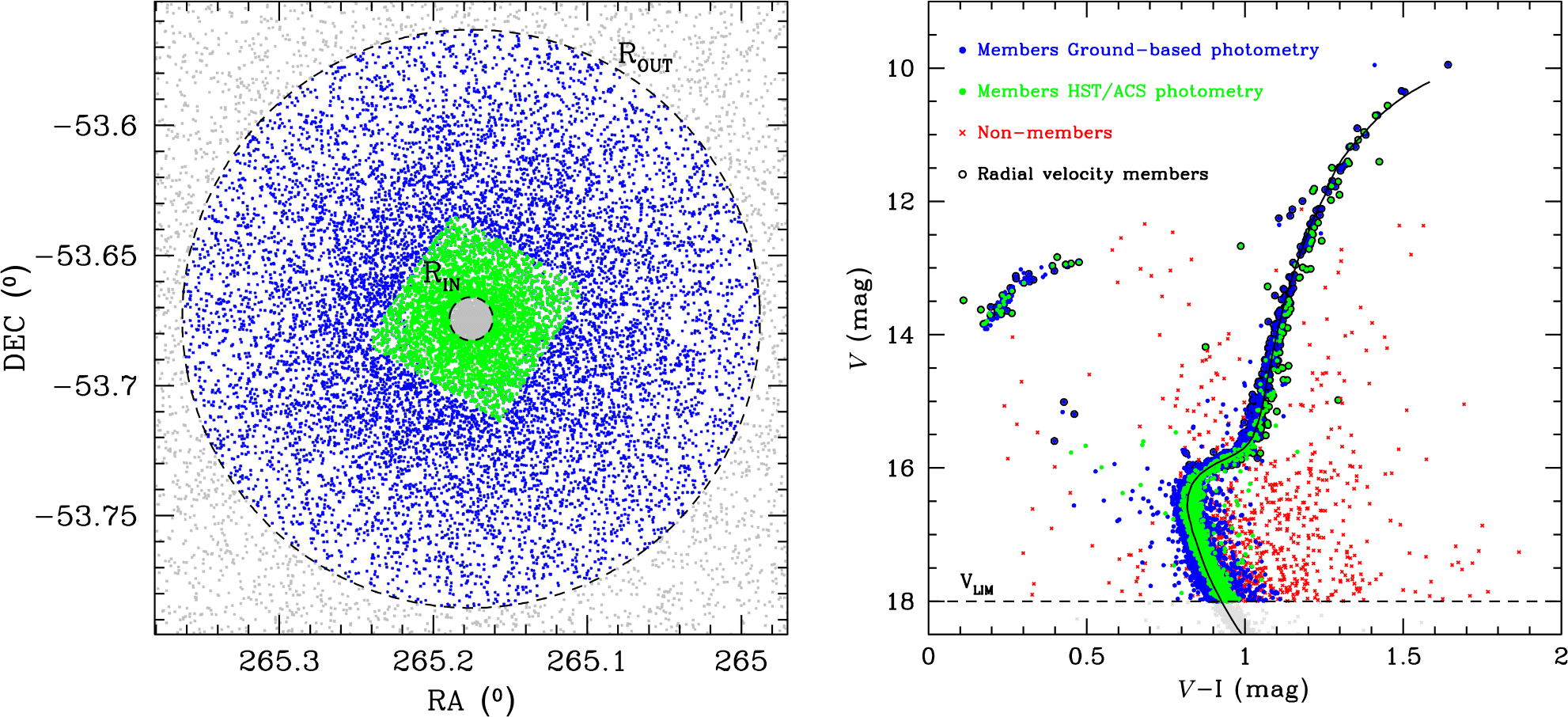
Figure 1. Illustration of our member star selection approach for the globular cluster NGC 6397. The left panel shows an 800”  $\times$ 800” arcsec field centred on the cluster. Stars selected from HST/ACS observations are shown in green, stars from the ground-based photometry of Stetson et al. (Reference Stetson, Pancino, Zocchi, Sanna and Monelli2019) in blue. The dashed circles show the limits of the field for which we determine the cluster luminosity. The right panel shows a CMD of NGC 6397 with a 12 Gyr old PARSEC isochrone overlayed as solid line. Blue and green circles depict cluster members, while red crosses depict stars classified as non-members based on their CMD position, Gaia proper motion, or radial velocity. The dashed line marks the lower limit down to which we use observed stars. Circles mark radial velocity members.
2.3. Selection of cluster members
Cluster members are selected from the photometric master catalogue based on three criteria: Position in the CMD, radial velocity, and Gaia proper motion. In order to select stars based on photometry, we fit PARSEC isochrones (Bressan et al. Reference Bressan, Marigo, Girardi, Salasnich, Dal Cero, Rubele and Nanni2012) to each cluster and use these to select main sequence and giant star members. Possible cluster members must either have a colour difference no larger than 2.5 times their photometric error from the best-fitting isochrone or have a colour difference less than a maximum value. We choose the maximum colour difference individually for each cluster based on the observed width of the RGB and the amount of background contamination. For most clusters, these values are usually around 0.20 mag. We also select stars as potential cluster members if they are located in the CMD in the region that correspond to horizontal-branch stars and blue stragglers. For a few clusters with strong and variable reddening, we first derive a de-reddened CMD by shifting stars along the reddening vector to a common main sequence and then identify cluster members in the de-reddened CMD.
Our second criterion for membership determination is the stellar radial velocities compiled by Baumgardt (Reference Baumgardt2017) and Baumgardt & Hilker (Reference Baumgardt and Hilker2018). Their data contain radial velocities and membership information for about 250 000 stars in the fields of globular clusters. We cross-match the positions of all stars that are classified as members based on CMD position with the radial velocities of Baumgardt & Hilker (Reference Baumgardt and Hilker2018) and keep only those stars that either have no radial velocity measurement or have a radial velocity that is within  $\pm 2.5 \sigma$ of the cluster mean velocity. Here the velocity dispersion
  $\sigma$ is calculated at the position of each star based on the best-fitting N-body model of Baumgardt & Hilker (Reference Baumgardt and Hilker2018).
We finally use the Gaia DR2 proper motions and parallaxes for membership determination. For stars that have passed the CMD and radial velocity tests, we cross-match their positions against the positions of stars in the Gaia catalogue and require that their proper motion is within  $2.5 \sigma$ of the mean cluster proper motion determined by Baumgardt et al. (Reference Baumgardt, Hilker, Sollima and Bellini2019). We also require that the star has a parallax that is compatible with the cluster parallax
  $p_{\rm CL}=1/d$ where d is the cluster distance given by Baumgardt & Hilker (Reference Baumgardt and Hilker2018). We keep all stars that have no Gaia counterparts. Stars without Gaia counterparts are either faint stars or stars in the centres of clusters that have a high chance of being cluster members due to the strong density contrast between cluster and field stars in the centre.
2.4. Magnitude determination
We calculate the total luminosity of the cluster members determined in the previous section according to:
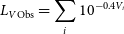 \begin{equation} L_{V {\rm Obs}} = \sum_i 10^{-0.4 V_i}\end{equation}
To derive the total cluster luminosities from  $L_{V Obs}$, we then need to correct
  $L_{V Obs}$ for faint stars not included in the photometry, cluster regions that are not covered by the photometry, and any background contamination remaining in the data.
We correct for incompleteness at the faint end by imposing a magnitude cut-off  $V_{\rm LIM}$ that is bright enough that the photometry is still complete for stars brighter than
  $V_{\rm LIM}$ but faint enough that stars fainter than
  $V_{\rm LIM}$ contribute only a small fraction of the cluster light. We usually choose
  $V_{\rm LIM}$ to be one or two magnitudes below the main-sequence turn over, depending on the quality of the photometry and the distance of the cluster. This guarantees that the directly measured bright stars already contribute between 80 and 90% of the total cluster luminosity. We estimate the contribution of the fainter stars based on the N-body models of Baumgardt & Hilker (Reference Baumgardt and Hilker2018). Baumgardt & Hilker (Reference Baumgardt and Hilker2018) ran a grid of about 3 000 N-body simulations and determined for each cluster the N-body model that produced the best fit to the observed stellar mass function at different radii, the observed surface density profile, and the observed velocity dispersion profile. Their simulations provide for each globular cluster a star-by-star model containing main-sequence, giant stars, and compact remnants. For each star, we use the bolometric luminosity, surface temperature, and metallicity from the N-body model and convert these into UBVRI magnitudes using the Kurucz (Reference Kurucz, Barbuy and Renzini1992) atmosphere models for nuclear burning stars and the bolometric corrections and colour indices calculated by Bergeron et al. (Reference Bergeron, Wesemael and Beauchamp1995) for white dwarfs. After the conversion, we calculate the total V band luminosity, of all stars
  $L_{{\rm Sim},A}$ and the one for only the bright stars
  $L_{{\rm Sim},B}$ with
  $V<V_{\rm Lim}$, and correct the observed cluster luminosity by
  $L_{V {\rm In}} = L_{V {\rm Obs}} \cdot L_{{\rm Sim},A}/L_{{\rm Sim},B}$. Varying
  $V_{\rm LIM}$ for a few nearby clusters with deep photometry shows that the derived luminosities vary by only about
  $\pm 0.03$ mag when decreasing the magnitude limit
  $V_{\rm LIM}$.
In order to estimate the contribution of the cluster parts that are either excluded due to crowding or not covered by the photometry to the total cluster luminosity, we again use the best-fitting N-body model of each cluster and calculate the total cluster luminosity  $L_{{\rm Sim},T}$ and the luminosity of the part that is covered by the photometry
  $L_{\rm Sim,In}$. We then calculate the total cluster luminosity by
  $L_{V, {\rm Tot}} = L_{V, {\rm In}} \cdot L_{{\rm Sim},T}/L_{\rm Sim,In}$. Once the total cluster luminosity has been calculated, we calculate the total magnitude of the cluster as
  $V = -2.5 \cdot \log_{10} L_{V, {\rm Tot}}$. For a few bulge clusters, background contamination is an issue even after selecting stars based on CMD position, radial velocities, and Gaia proper motions and parallaxes. In order to correct the cluster luminosity for background stars, we integrate the cluster profile out to large radii so that we can determine the surface brightness of background stars and then subtract the total luminosity of the background stars from the cluster luminosity. Table B.1 presents the total cluster luminosities that we derive this way. It also presents the absolute magnitudes that we calculate from the apparent magnitudes using the extinction values from Harris (Reference Harris1996) as well as the cluster distances from Baumgardt et al. (Reference Baumgardt, Hilker, Sollima and Bellini2019) and the radii containing 10% and 50% of the cluster light in projection together with the surface brightness at these radii.
We estimate the error of the cluster luminosity as follows: For clusters where we have no photometry in the Johnson–Cousins system with which to correct the HST magnitudes, we assume an error of  $\Delta V = 0.10$ mag on the total cluster luminosity. We assume that this error drops to
  $\Delta V = 0.04$ mag for clusters where we have ground-based V band magnitude measurements. The latter value is equal to the maximum zero-point uncertainty estimated by Stetson et al. (Reference Stetson, Pancino, Zocchi, Sanna and Monelli2019) for their photometry. We also assume that the correction factors
  $f_{\rm Bright} = L_{{\rm Sim},A}/L_{{\rm Sim},B} - 1$ and
  $f_{\rm Field} = L_{{\rm Sim},T}/L_{\rm Sim,In}-1$ have 10% relative errors, i.e. if
  $f_{\rm Bright} = 0.20$, we assume that the corresponding correction of the cluster luminosity has a relative error of 2%, leading to a 0.022 mag uncertainty of the total cluster magnitude. We also assume that the global mass function slopes
  $\alpha$ determined by Baumgardt & Hilker (Reference Baumgardt and Hilker2018) have uncertainties of
  $\pm$0.20. Experiments show that the final cluster luminosity changes by 0.02 mag for a change of
  $\alpha$ of 0.20. Finally, for those clusters where we subtracted a background contribution, we vary the assumed background level by 10% and assume an additional magnitude error equal to the change in total cluster magnitude caused by this variation of the assumed background level. The total magnitude error is then calculated combining the various magnitude uncertainties, which we assume to be statistically independent. The magnitude errors are also given in Table B.1. For the best observed clusters, we can achieve errors better than 0.05 mag, i.e. luminosities accurate to about 5%.
3. Results
3.1. Apparent magnitudes
Figure 2 and Table 1 compare the apparent magnitudes derived here with those given in the 2010 version of Harris (Reference Harris1996), (H10) Dalessandro et al. (Reference Dalessandro, Schiavon, Rood, Ferraro, Sohn, Lanzoni and O’Connell2012) (D12), and McLaughlin & van der Marel (Reference McLaughlin and van der Marel2005) (M05). The magnitudes from Harris (Reference Harris1996) are mainly derived from aperture photometry, while McLaughlin & van der Marel (Reference McLaughlin and van der Marel2005) derived magnitudes through an integration of the surface density profiles of Trager et al. (Reference Trager, King and Djorgovski1995). Dalessandro et al. (Reference Dalessandro, Schiavon, Rood, Ferraro, Sohn, Lanzoni and O’Connell2012) derived total magnitudes from data of the GALEX satellite. Hence, all estimates use different input data and are more or less independent of each other. We therefore average the literature estimates and compare them with the magnitudes derived here in the last row of Table 1. Only clusters that have at least two magnitude determinations in the literature are used in the last row.
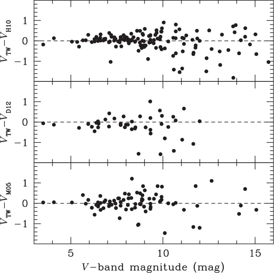
Figure 2. Difference in the total magnitudes between this work and (from top to bottom) the 2010 version of Harris (Reference Harris1996) (H10), Dalessandro et al. (Reference Dalessandro, Schiavon, Rood, Ferraro, Sohn, Lanzoni and O’Connell2012) (D12), and McLaughlin & van der Marel (Reference McLaughlin and van der Marel2005) (M05). The differences increase for fainter clusters and can reach up to two magnitudes for individual clusters.
The literature values show good agreement with our measurements only for bright clusters with  $V<8$ mag, where the average difference is close to zero and the typical deviation for individual clusters is about 0.20 mag. For clusters with total magnitudes fainter than 8 mag, the differences quickly increase and can be as large as 2 mag for some clusters fainter than
  $V=11$ mag. For all magnitude ranges, the differences are much larger than what we expect based on our magnitude errors, indicating that the differences are mainly due to inaccuracies in the literature magnitudes. Interestingly, averaging the literature magnitudes already leads to significantly smaller scatter than derived from the individual data sets. A closer examination shows that the most discrepant clusters are often relatively low-mass clusters like Pal 11 (
 $M=1.0 \cdot 10^4\ \mathrm{M}_\odot$), Ter 8 (
 $M=5.9 \cdot 10^4\ \mathrm{M}_\odot$), or Arp 2 (
 $M=3.9 \cdot 10^4\ \mathrm{M}_\odot$). Since most of these clusters are located in areas of low field-star contamination, have both deep and ground-based photometry, and have proper motions that clearly separate the cluster from the field stars, we regard our total magnitudes as very reliable. The reason for the strong discrepancy with the literature values could be that the aperture photometry measurements and the surface brightness profiles of Trager et al. (Reference Trager, King and Djorgovski1995) have excluded bright giant stars in order to obtain smooth density profiles. This could explain why for the faintest clusters our magnitude values are on average smaller (meaning we derive larger total luminosities) compared to the literature values. It could also explain why more massive and brighter clusters show better agreement, since the effect of single bright stars is smaller in more massive clusters. The remaining clusters that show large differences are mostly bulge clusters like NGC 6256, NGC 6453, or NGC 6749 which are located in fields with a large background density of stars. Since we use Gaia proper motions to clean the CMDs from field stars, we again expect our magnitudes to be more reliable than the literature ones.
Table 1. Mean differences and standard deviation around the mean between our photometry and literature values for three different magnitude ranges.
3.2. Absolute cluster magnitudes
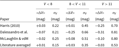
In order to convert the apparent magnitudes to absolute ones, we use the cluster distances from Baumgardt et al. (Reference Baumgardt, Hilker, Sollima and Bellini2019) and the  $E(B-V)$ values given by Harris (Reference Harris1996). Figure 3 depicts the distribution of absolute magnitudes of globular clusters that we derive this way, split up into the full sample (upper panel), inner clusters with galactocentric distances
  $R_{\rm GC}<15$ kpc (middle panel), and outer clusters with
  $R_{\rm GC}>15$ kpc (lower panel). Fitting a Gaussian to the distribution, we obtain a mean magnitude of
  $M_V=-7.13$ and a width of
  $\sigma_V=1.47$ for the full cluster sample. Our mean absolute magnitude is about 0.2–0.3 mag lower, and the width is significantly higher than what has been found previously (e.g. Secker Reference Secker1992; Di Criscienzo et al. Reference Di Criscienzo, Caputo, Marconi and Musella2006). The main reason for the difference is the many low-mass clusters that have been discovered in recent years: For example, out of the 15 globular clusters known today that are not included in the sample of Di Criscienzo et al. (Reference Di Criscienzo, Caputo, Marconi and Musella2006), 14 have absolute luminosities below the mean. It is therefore likely that the average luminosity of MW globular clusters could be lower since our census of globular clusters in the inner parts of the Milky Way is probably still not complete (Minniti et al. Reference Minniti2017). The middle and lower panels of Figure 3 split the cluster sample into an inner sample inside
  $R_{\rm GC}=15$ kpc and an outer one. For the inner clusters, we obtain a mean of
  $M_V=-7.39$ with a width of
  $\sigma_V=1.19$. Both values do not seem to depend on the radial range that we consider, indicating that the globular cluster luminosity function is invariant in the inner parts of the Milky Way. In contrast, the outer clusters have a significantly lower mean luminosity of
  $M_V=-6.40$ and a much larger width. Huxor et al. (Reference Huxor2014) found evidence that the outer globular cluster system of the Andromeda Galaxy has a bi-model distribution in luminosity, with a second peak at
  $M_V-5.5$. The Milky Way globular cluster system could show a similar bi-modality, with one peak at around
  $M_V=-8$, similar to the inner globular clusters, and a second peak around
  $M_V=-6$. Huxor et al. (Reference Huxor2014) also speculated that the bright outer-halo clusters in M31 formed in situ, while the clusters in the fainter peak are accreted from dwarf galaxies. Current orbital data on the Milky Way globular clusters, however, do not support this conclusion: Out of the 14 globular clusters that are at distances
  $R_G>$15 kpc and that are brighter than
  $M_V=-7.0$, all are associated with a dwarf galaxy progenitor (Gaia-Enceladus, Sagittarius or Helmi Streams) in the recent study by Massari et al. (Reference Massari, Koppelman and Helmi2019). In contrast, among the 23 outer clusters fainter than
  $M_V=-7.0$, only 9 are considered securely and 3 are possibly associated with a dwarf galaxy progenitor according to Massari et al. (Reference Massari, Koppelman and Helmi2019). Hence, many of the faint globular clusters could have formed in situ in the halo of the Milky Way without a connection to a dwarf galaxy. Alternatively, they could be associated with dwarf galaxies that have not yet been discovered.
Figure 3. Distribution of absolute magnitudes of Milky Way globular clusters. The top panel shows the full distribution, the middle panel the distribution of inner clusters with  $R_G<15$ kpc, and the lower panel the distribution of outer clusters with
  $R_G>15$ kpc. The distribution of outer clusters contains a significantly larger fraction of low-luminosity clusters.
3.3. Cluster M/LV ratios
Figure 4 compares the mass-to-light ratios that we derive from our magnitudes with the  $M/L_V$ ratios that we derive from the literature averaged V-band luminosities. In order to calculate the cluster mass-to-light ratios, we use the cluster masses and distances from Baumgardt et al. (Reference Baumgardt, Hilker, Sollima and Bellini2019) and the extinction values given by Harris (Reference Harris1996). We only plot clusters that have relative mass uncertainties
  $\Delta M/M<0.2$ in Figure 4 in order to be able to better judge the quality of the cluster luminosities. For the same reason, we restrict ourselves to clusters with extinction values
  $E(B-V)<1.0$ since for highly reddened clusters differential extinction or uncertainties in the reddening could introduce additional uncertainties. We obtain an average mass-to-light ratio of
  $M/L_V=1.83 \pm 0.03\ {\rm M}_\odot/{\rm L}_\odot$ and a standard deviation of
  $\sigma_{M/L}=0.24 \pm 0.03\ {\rm M}_\odot/{\rm L}_\odot$ around the mean using our magnitudes compared to
  $M/L_V=1.92 \pm 0.05\ {\rm M}_\odot/{\rm L}_\odot$ and
  $\sigma_{M/L}=0.49 \pm 0.05\ {\rm M}_\odot/{\rm L}_\odot$ that we derive from the literature magnitudes. Hence, while the average mass-to-light ratio changes by only 0.1
  ${\rm M}_\odot/{\rm L}_\odot$, we obtain a much more uniform
  $M/L_V$ distribution using our magnitudes. In particular, using our magnitudes, no clusters have mass-to-light ratios
  $M/L_V>2.5\ {\rm M}_\odot/{\rm L}_\odot$ or
  $M/L_V<1\ \mathrm{M}_\odot/{\rm L}_\odot$, which would be hard to explain using standard isochrones (see Section 3.2).
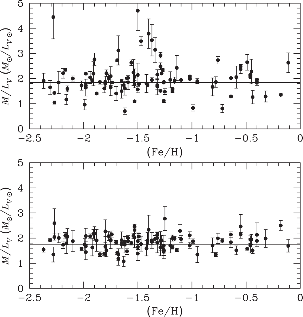
Figure 4.  $M/L_V$ mass-to-light ratios derived using masses and distances from Baumgardt et al. (Reference Baumgardt, Hilker, Sollima and Bellini2019), extinction values from Harris (Reference Harris1996), and literature averaged V-band luminosities (top panel). The bottom panel shows the mass-to-light ratios derived with the same data but our V band magnitudes. The resulting
  $M/L_V$ ratios cover a much smaller scatter around the mean value (marked by a solid line).
The  $M/L$ ratio of a cluster is influenced by several different processes: First, stellar evolution leads to an increase of the
  $M/L$ ratio with time as massive and bright stars, which are contributing to the total cluster light more than to the cluster mass, are constantly being turned into compact remnants. According to the PARSEC isochrones (Bressan et al. Reference Bressan, Marigo, Girardi, Salasnich, Dal Cero, Rubele and Nanni2012), stellar evolution should increase the
  $M/L_V$ ratio of a globular cluster by about 0.3
  ${\rm M}_\odot/{\rm L}_\odot$ when the cluster age increases from
  $T=10$ Gyr to
  $T=13.5$ Gyr, with only a weak dependence of this increase on metallicity. Second, the stellar mass function of a cluster changes as a result of mass segregation, which lets massive stars sink into the centre and moves low-mass stars towards the outer cluster parts where they are preferentially removed due to an external tidal field. Baumgardt & Makino (Reference Baumgardt and Makino2003) found by means of N-body simulations that this process leads initially to a decrease of the cluster
  $M/L$ ratio since low-mass stars mainly contribute to the cluster mass and only little to the overall cluster light, followed by an increase very close to final dissolution when mainly compact remnants are left in the cluster. Baumgardt & Makino (Reference Baumgardt and Makino2003) found a maximum decrease of the
  $M/L$ ratio of about
  $\Delta M/L_V=0.5$ to 0.7 due to mass loss. A decrease of the cluster
  $M/L$ ratio during the evolution was also found by Bianchini et al. (Reference Bianchini, Sills, van de Ven and Sippel2017), although they found that the ejection of dark remnants is also important in changing the
  $M/L$ ratio of a star cluster. Finally,
  $M/L$ ratios also depend on the metallicity of a cluster. Maraston (Reference Maraston1999) predicted an increase of the V-band
  $M/L$ ratio by a factor three when increasing the metallicity from [Fe/H]
  $=-0.5$ to [Fe/H]
  $=+0.3$.
Figures 5 and 6 depict the dependence of the  $M/L$ ratios that we derive from our magnitudes on the cluster age and mass function slope
  $\alpha$. Similar to the previous plots, we show only clusters that have relative mass errors
  $\Delta M/M<0.2$ and reddening values
  $E(B-V)<1.0$. We also divide the sample into low-metallicity clusters with [Fe/H]
  $<-1.5$ and high-metallicity clusters with [Fe/H]
  $>-1.5$ to reduce the dependency on metallicity. We have taken the cluster ages in Figure 5 mainly from VandenBerg et al. (Reference VandenBerg, Brogaard, Leaman and Casagrande2013), or, if a cluster was not studied by them, from the literature. We obtain highly significant positive Spearman rank-order coefficients
  $r_s$ for both metallicity ranges. Also a linear fit of the form
  $M/L_V = x+y \cdot T_{\rm Age}$ gives positive slopes y for both metallicity ranges, indicating that cluster
  $M/L$ ratios increase with age. The increase seen when going from
  $T=10$ Gyr to
  $T=13.5$ Gyr is about 0.45
  ${\rm M}_\odot/{\rm L}_\odot$ for both metal-poor and metal-rich clusters, in agreement with the predicted change based on stellar isochrones.
Figure 6 depicts the  $M/L_V$ ratios against the mass function of the clusters, taken from Baumgardt et al. (Reference Baumgardt, Hilker, Sollima and Bellini2019). We obtain a weak anti-correlation between the mass-to-light ratio of a cluster and its mass function slope
  $\alpha$ only for the metal-poor clusters. For the metal-rich clusters, there is no visible correlation. One reason for the lack of a correlation for metal-rich clusters could be that either the mass or mass function measurements for these have large errors since many of these clusters are located in the bulge, which makes observations of them more difficult. Alternatively, clusters could start with different initial mass functions, so the present-day differences in the MF slope
  $\alpha$ are not due to dynamical evolution.
3.4. Contribution of different stars to the total magnitudes
Table 2 shows the contribution of stars in different evolutionary stages to the total V-band magnitudes. We have split stars into main sequence stars (MS), horizontal branch stars (HB), blue stragglers (BS), and red giant branch stars (RGB), where the RGB stars include asymptotic giant branch and sub-giant branch stars as well. As an example, Figure 7 depicts the division of stars for two clusters, NGC 6528 and NGC 7078. We have analysed six clusters, roughly equally spaced in metallicity between [Fe/H] =  $-2.37$ to [Fe/H] =
  $-0.11$, thereby encompassing the range of metallicities seen for Galactic globular clusters. We again use our N-body models to correct for main-sequence stars too faint to be seen in the observations.
Table 2. Relative contribution of stars in different evolutionary stages to the total V-band magnitudes for six clusters.
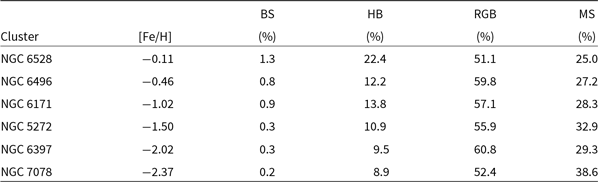
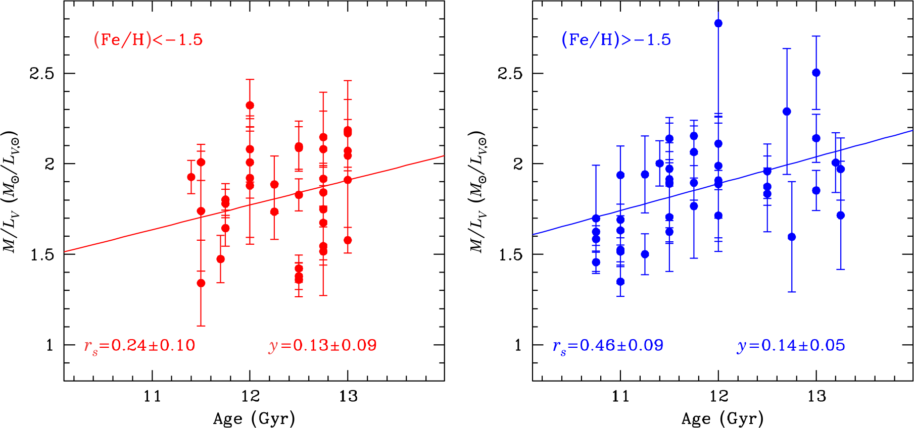
Figure 5. Dependence of mass-to-light ratio on the cluster ages for two different metallicity ranges. The  $M/L$ ratio increases as a function of age in agreement with theoretical predictions. The plots also show the Spearman rank-order coefficient
  $r_s$ as well as the slope y of the best-fitting linear fit to the data.
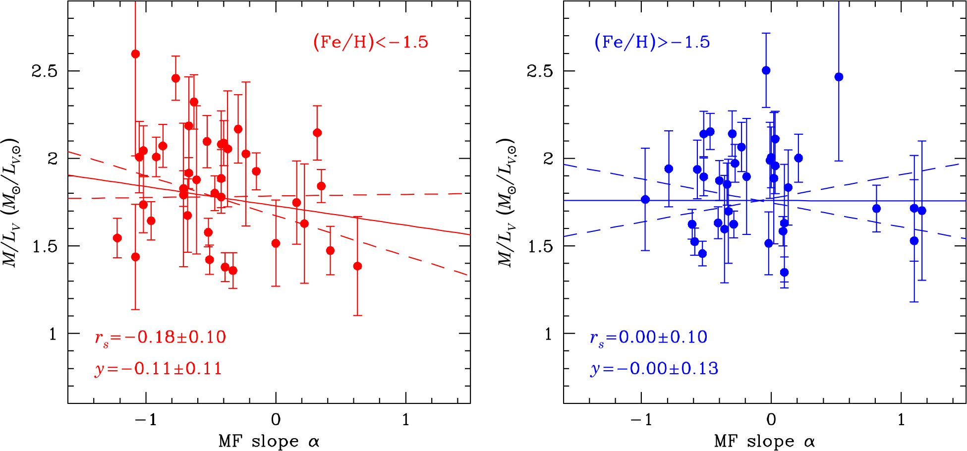
Figure 6. Same as Figure 5 but this time showing the dependence of mass-to-light ratio on the mass function of clusters.
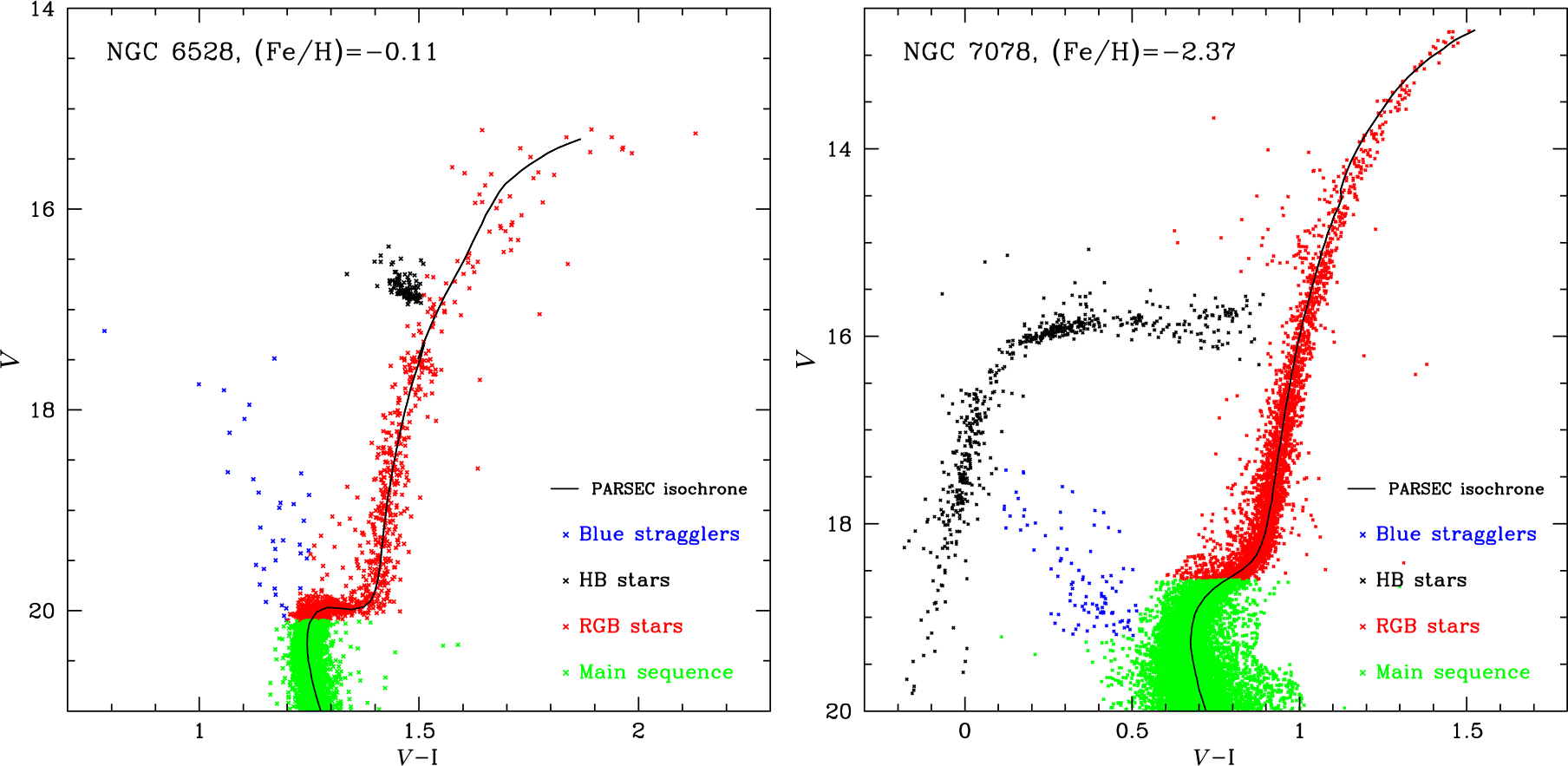
Figure 7. Illustration of our division of stars into different evolutionary stages for the high metallicity cluster NGC 6528 (left panel) and the low metallicity cluster NGC 7078 (right panel). Stars are split into blue stragglers (blue), horizontal branch stars (HB, black), red giant branch stars (RGB, red), and main sequence stars (green). Only stars that pass the various membership criteria detailed in Section 2 are shown.
It can be seen that blue stragglers contribute only about  $\sim$1% to the total cluster light, with a strong increase of their contribution towards higher metallicity. The fraction of light from HB stars is also increasing with metallicity, while the fraction of light coming from the RGB is roughly constant at around 55%. The increase of the fraction of light in HB stars at increasing metallicity confirms predictions by stellar evolution models (e.g. Renzini & Buzzoni Reference Renzini and Buzzoni1986), which predict such an increase as a result of the shorter evolutionary timescales on the RGB stars. There also seems to be a slight decrease of the fraction of light from MS stars with metallicity; however, this decrease could also be driven by other factors like a change of the internal mass function of the clusters. A larger sample would be needed to disentangle the different effects.
3.5. Comparison with stellar evolution models
Figure 8 depicts the ratio of the  $M/L_V$ values that we derive from our apparent cluster magnitudes with the predictions of stellar evolution models. Shown are predictions from version 1.2 of the MIST isochrones (Paxton et al. Reference Paxton2015; Dotter Reference Dotter2016; Choi et al. Reference Choi, Dotter, Conroy, Cantiello, Paxton and Johnson2016), version 1.2 of the PARSEC isochrones (Bressan et al. Reference Bressan, Marigo, Girardi, Salasnich, Dal Cero, Rubele and Nanni2012), and predictions from the DARTMOUTH isochrones (Dotter et al. Reference Dotter, Chaboyer, Jevremović, Kostov, Baron and Ferguson2008a). For each stellar evolution model, we created a two-dimensional grid of isochrones in age and metallicity. Isochrones were spaced by 0.5 Gyr between 10 Gyr and 13.5 Gyr in age and by
  $\Delta$ [Fe/H] = 0.10 between [Fe/H] =
  $-2.50$ and [Fe/H] = 0.0 in metallicity. For each cluster age, metallicity, and stellar evolution model, we then distributed
  $5 \cdot 10^5$ stars following the mass functions given in Baumgardt & Hilker (Reference Baumgardt and Hilker2018) and then used the isochrones to calculate the total luminosity, total mass, and
  $M/L$ ratio of each model. We thus obtained a grid of 1 456 models giving the
  $M/L_V$ ratio of star clusters as a function of cluster age, metallicity, and internal mass function for each stellar evolution model. We then linearly interpolate in this grid of models to predict the expected mass-to-light ratio of each globular cluster given its mass function, metallicity, and cluster age.
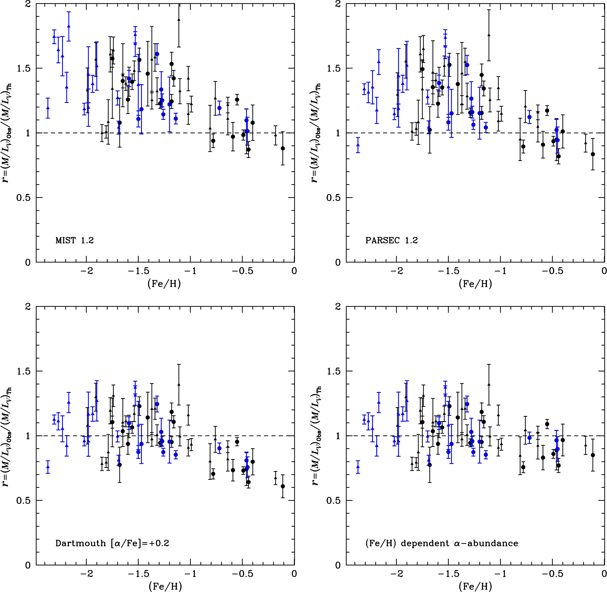
Figure 8. Ratio of the measured  $M/L_V$ ratios to the
  $M/L_V$ ratio predicted by different stellar-evolution models as a function of the cluster metallicity. Shown is a comparison against MIST isochrones (top left), PARSEC isochrones (top right), Dartmouth isochrones with enhanced
  $\alpha$ element ratios of [
 $\alpha$/Fe]=+0.2 and a model in which the
  $\alpha$-element abundances decrease for metal-rich clusters (lower right).
Figure 8 compares the ratio of the observed  $M/L_V$ ratios to the theoretically predicted ones. It can be seen that the predictions of the MIST and PARSEC isochrones are very similar. Both reproduce the observed mass-to-light ratios of metal-rich clusters quite well, but predict higher than observed
  $M/L_V$ ratios for the metal-poor clusters. The mismatch between observed and predicted
  $M/L_V$ ratios of metal-rich globular clusters noted by Strader et al. (Reference Strader, Caldwell and Seth2011) is therefore mainly due to the fact that Strader et al. (Reference Strader, Caldwell and Seth2011) assumed a Kroupa or Salpeter type mass function for the clusters, while the data for the Milky Way globular clusters indicate that they follow much shallower mass functions. At the moment, the data do not support a metallicity-dependent top-heavy IMF as suggested by Zonoozi et al. (Reference Zonoozi, Haghi and Kroupa2016), although we cannot rule out any such variation either.
A possible reason for the mismatch between predicted and observed  $M/L_V$ ratios of metal-poor globular clusters could be that the isochrone models considered a solar-abundance pattern, while metal-poor stars are known to be enriched in
  $\alpha$-elements (Pritzl et al. Reference Pritzl, Venn and Irwin2005). The lower-left hand figure therefore compares our observed
  $M/L_V$ ratios with DARTMOUTH isochrones that have an
  $\alpha$-element enhancement of
  $[\alpha$/Fe]=
 $+0.2$. We use DARTMOUTH isochrones since for MIST and PARSEC isochrones only solar abundance models are available. It can be seen that for
  $\alpha$-enhanced isochrones, the predicted
  $M/L_V$ ratios of metal-poor clusters with [Fe/H]
 $<-1$ are in agreement with the observed ones, while the metal-rich clusters now have too low
  $M/L_V$ ratios. However, there are indications that the
  $\alpha$-element enhancement of globular clusters decreases for clusters with [Fe/H]
 $>-1$ down to solar values (e.g. Ferraro et al. Reference Ferraro, Messineo, Fusi Pecci, de Palo, Straniero, Chieffi and Limongi1999; Pritzl et al. Reference Pritzl, Venn and Irwin2005). Figure 3 in Horta et al. (Reference Horta2020), for example, shows that clusters with [Fe/H]
 $ <-0.7$ have more or less constant [Si/Fe] of about [Si/Fe]
 $=+0.25$, followed by a downturn in the [Si/Fe] values similar to what is seen for field stars. The two most metal-rich clusters in their sample (Liller 1 and Pal 10) have [Si/Fe] of
  $0.01 \pm 0.05$ and
  $0.0 \pm 0.10$, respectively, i.e., they are compatible with a solar abundance ratio. A downturn of the
  $\alpha$-element abundances for metal-rich globular clusters is also predicted based on cosmological simulations (e.g. Hughes et al. Reference Hughes, Pfeffer, Martig, Reina-Campos, Bastian, Crain and Kruijssen2020).
We therefore adopt an  $\alpha$-element distribution with
  $[\alpha$/Fe]
 $=+0.2$ for clusters with [Fe/H]
 $\,<-0.8$ followed by a linear decrease down to
  $[\alpha$/Fe]
 $\,=+0.0$ for [Fe/H] = 0.0 and interpolate in our grid between the
  $[\alpha$/Fe] =
  $+0.2$ DARTMOUTH models and the PARSEC models depending on the
  $\alpha$-element enhancement of each cluster. The resulting
  $M/L_V$ ratios are shown in the lower right corner. It can be seen that we now obtain an excellent agreement between the observed and expected mass-to-light ratios at all metallicities.
4. Conclusion
We have derived new V-band magnitudes of 153 Galactic globular clusters by summing up the magnitudes of their individual members stars derived from HST and ground-based photometry and correcting the derived magnitudes for missing faint stars and spatial incompleteness. In order to differentiate between cluster and field stars, we have made use of the positions of stars in colour-magnitude diagrams, available radial-velocity information, and proper motions and parallaxes from Gaia DR2. Our V-band magnitudes show good agreement with published literature magnitudes for bright clusters with  $V<8$ mag. For fainter clusters, typical differences are of order 0.5 mag with individual clusters showing differences of up to 2 mag.
Our V-band magnitudes lead to a mean mass-to-light ratio of  $M/L_V=1.83$ and a scatter of
  $\sigma_V=0.24\ {\rm M}_\odot/{\rm L}_\odot$ around the mean, significantly smaller than the scatter obtained with literature magnitudes. In agreement with Strader et al. (Reference Strader, Caldwell and Seth2011), we find no dependence of the average mass-to-light ratio of a cluster with metallicity. We find evidence that the mass-to-light ratios of globular clusters are increasing with cluster age, in agreement with theoretical predictions. We also find good agreement between the derived mass-to-light ratios with the expected ones from stellar isochrones if the mass function of the clusters is taken into account. PARSEC and MIST stellar isochrones with a solar-abundance pattern for
  $\alpha$-elements are able to reproduce the mass-to-light ratios only for clusters with [Fe/H]
  $>-1.0$, but predict too high mass-to-light ratios for the more metal-poor clusters. However, using
  $\alpha$-enhanced DARTMOUTH isochrones with
  $[\alpha$/Fe]
  $=+0.2$ leads to a good agreement of observed and predicted
  $M/L$ ratios. There is, therefore, no evidence for a significant amount of dark matter inside the main body of globular clusters as has been previously suggested (Baumgardt & Mieske Reference Baumgardt and Mieske2008; Wirth, Bekki, & Hayashi Reference Wirth, Bekki and Hayashi2020). However, the data do not rule out dark matter haloes surrounding globular clusters or a small amount (of order 20% of the total mass or less) of dark matter inside the clusters.
We finally find that globular clusters at galactocentric distances  $R_G>15$ kpc have on average about one magnitude lower absolute magnitudes than clusters inside this radius. This could be either due to the weaker tidal field in the outer parts of the Milky Way, which increases the lifetime of low mass clusters to more than a Hubble time, or due to the fact that low-mass clusters in the inner Milky Way have not yet been found due to large reddening and the strong background density of stars. About half of the low-luminosity clusters in the outer parts are not connected to any known dwarf galaxy or any known past merger events that are thought to have happened in the early Milky Way, indicating that they either formed in situ or are connected to so far undiscovered dwarf galaxies.
In the future, determining total magnitudes, cluster colours, and  $M/L$ ratios in other wavelength bands will be useful for tests of stellar evolution and galactic studies. Given our photometric data and the fact that we already have determined the cluster members, this task should also be straightforward to implement. Our photometry should also help determine the contribution of stars in different evolutionary stages (RGB, HB, main sequence, and blue stragglers) to the total magnitudes in the different bands. The caveat, however, is that individual stellar photometry in bands other than the V band is currently only available for a subset of Galactic clusters.
Acknowledgements
The authors thank Sylvie Beaulieu, Aaron Dotter, Matthias Frank, Edoardo P. Lagioia, Domenico Nardiello, Stefano Oliveira de Souza, Soeren S. Larsen, Sebastian Kamann, Jeffrey Simpson, and Daniel Weisz for sharing their globular cluster photometry with us. The authors also acknowledge the work by Peter Stetson in deriving wide-field, ground-based photometry of globular clusters and making his data public before publication. The authors finally thank Mirek Giersz and Jarrod Hurley for making a FORTRAN code available to us that converts bolometric luminosities and temperatures into absolute magnitudes in the Johnson–Cousins system. Based on observations made with the NASA/ESA Hubble Space Telescope, obtained from the data archive at the Space Telescope Science Institute. STScI is operated by the Association of Universities for Research in Astronomy, Inc. under NASA contract NAS 5-26555. This research has made use of the SIMBAD database, operated at CDS, Strasbourg, France. This work has made use of data from the European Space Agency (ESA) mission Gaia (https://www.cosmos.esa.int/gaia), processed by the Gaia Data Processing and Analysis Consortium (DPAC, https://www.cosmos.esa.int/web/gaia/dpac/consortium). Funding for the DPAC has been provided by national institutions, in particular the institutions participating in the Gaia Multilateral Agreement.
A. Input photometry used to derive the apparent magnitudes of globular clusters
Table A.1. Input photometry used to calculate the total magnitudes of globular clusters.

B. Derived magnitudes and mass-to-light ratios
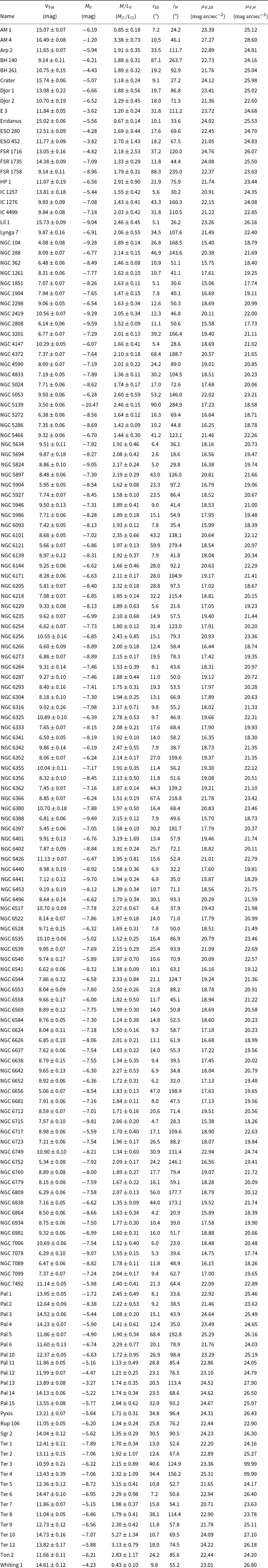
Table B.1. Apparent and absolute V-band magnitudes, mass-to-light ratios, and the radii containing 10% and half the total cluster light in projection together with the surface density brightnesses at these radii for all clusters in this study.