
Abstract
Species distribution modelling (SDM) is a valuable tool for predicting the potential distribution of invasive species across space and time. Maximum entropy modelling (MaxEnt) is a popular choice for SDM, but questions have been raised about how these models are developed. Without biologically informed baseline assumptions, complex default SDM models could be selected, even though alternative settings may be more appropriate. Here we explored the effects of various SDM design strategies on distribution mapping of four forest invasive species (FIS) in Canada. We found that if we ignored the underlying FIS biology such as use of biologically relevant predictors, appropriate feature selection and inclusion of dispersal and biotic interactions when we developed our SDMs, we obtained complex SDMs (default) that provided an incomplete picture of the potential FIS invasion. We recommend simplifying SDM complexity and including biologically informed assumptions to achieve more accurate dispersal predictions, particularly when projecting FIS spread across time. We strongly encourage SDM users to perform species-specific tuning when modeling FIS distributions with MaxEnt to determine the best SDM design.


References
Allouche O, Tsoar A, Kadmon R (2006) Assessing the accuracy of species distribution models: prevalence, kappa and the true skill statistic (TSS). J App Ecol 43:1223–1232. https://doi.org/10.1111/j.1365-2664.2006.01214.x
Anderson RP, Gonzalez I (2011) Species-specific tuning increases robustness to sampling bias in models of species distributions: an implementation with Maxent. Ecol Model 222:2796–2811. https://doi.org/10.1016/j.ecolmodel.2011.04.011
Andresen JA, McCullough DG, Potter BE, Koller CN, Bauer LS, Lusch DP, Ramm CW (2001) Effects of winter temperatures on gypsy moth egg masses in the Great Lakes region of the United States. Agric For Meteorol 110(2):85–100. https://doi.org/10.1016/s0168-1923(01)00282-9
Araújo MB, Guisan A (2006) Five (or so) challenges for species distribution modelling. J Biogeogr 33:1677–1688. https://doi.org/10.1111/j.1365-2699.2006.01584.x
Bancroft JS, Smith MT (2005) Dispersal and influences on movement for Anoplophora glabripennis calculated from individual mark-recapture. Entomol Exp Appl 116:83–92. https://doi.org/10.1111/j.1570-7458.2005.00320.x
Barbet-Massin M, Jiguet F, Albert CH, Thuiller W (2012) Selecting pseudo-absences for species distribution models: how, where and how many? Methods Ecol Evol 3:327–338. https://doi.org/10.1111/j.2041-210x.2011.00172.x
Barbosa FG, Schneck F, Melo AS (2012) Use of ecological niche models to predict the distribution of invasive species: a scientometric analysis. Braz J Biol 72:821–829. https://doi.org/10.1590/s1519-69842012000500007
Barry S, Elith J (2006) Error and uncertainty in habitat models. J Appl Ecol 43:413–423. https://doi.org/10.1111/j.1365-2664.2006.01136.x
Bean WT, Stafford R, Brashares JS (2012) The effects of small sample size and sample bias on threshold selection and accuracy assessment of species distribution models. Ecography 35:250–258
Brasier CM, Mehrotra MD (1995) Ophiostoma himal-ulmi sp. nov., a new species of Dutch elm disease fungus endemic to the Himalayas. Mycol Res 99:205–215. https://doi.org/10.1016/s0953-7562(09)80887-3
Brown JL (2014) SDMtoolbox: a python-based GIS toolkit for landscape genetic, biogeographic and species distribution model analyses. Methods Ecol Evol 5:694–700. https://doi.org/10.1111/2041-210x.12200
Brown JL, Bennett JR, French CM (2017) SDMtoolbox 2.0: the next generation Python-based GIS toolkit for landscape genetic, biogeographic and species distribution model analyses. PeerJ 5:e4095
Browning M, Englander L, Tooley PW, Berner D (2008) Survival of Phytophthora ramorum hyphae after exposure to temperature extremes and various humidities. Mycologia 100(2):236–245
Chapman D, Pescott OL, Roy HE, Tanner R (2019) Improving species distribution models for invasive non-native species with biologically informed pseudo-absence selection. J Biogeogr 46:1029–1040. https://doi.org/10.1111/jbi.13555
Cobos ME, Peterson TA, Barve N, Osorio-Olvera L (2019) kuenm: an R package for detailed development of ecological niche models using Maxent. PeerJ 7:e6281. https://doi.org/10.7717/peerj.6281
Colautti RI, Bailey SA, van Overdijk CDA, Amundsen K, MacIsaac HJ (2006) Characterized and projected costs of nonindigenous species in Canada. Biol Invasions 8:45–59. https://doi.org/10.1007/s10530-005-0236-y
Commonwealth Agricultural Bureaux International (CABI) (2019a) Anoplophora glabripennis (Asian longhorned beetle). https://www.cabi.org/isc/datasheet/5557#71A9CFAD-8527-4217-9678-41E0B01EE83A Accessed 26 June 2020
Commonwealth Agricultural Bureaux International (CABI) (2019b) Lymantria dispar (gypsy moth). https://www.cabi.org/isc/datasheet/31807#toDistributionMaps Accessed 26 June 2020
Commonwealth Agricultural Bureaux International (CABI) (2019c) Ophiostoma ulmi (Dutch elm disease). https://www.cabi.org/isc/datasheet/12165#D451998E−7E25-40C0-8BCB-7F9C88580E02 Accessed 26 June 2020
Commonwealth Agricultural Bureaux International (CABI) (2019d) Phytophthora ramorum (sudden oak death (SOD)). https://www.cabi.org/isc/datasheet/40991 Accessed 26 June 2020
Condeso TE, Emiko Condeso T, Meentemeyer RK (2007) Effects of landscape heterogeneity on the emerging forest disease sudden oak death. J Ecol 95:364–375. https://doi.org/10.1111/j.1365-2745.2006.01206.x
Cushman JH, Cushman J, Meentemeyer RK (2008) Multi-scale patterns of human activity and the incidence of an exotic forest pathogen. J Ecol 96:766–776. https://doi.org/10.1111/j.1365-2745.2008.01376.x
Davidson JM, Wickland AC, Patterson HA, Falk KR, Rizzo DM (2005) Transmission of Phytophthora ramorumin mixed-evergreen forest in California. Phytopathology 95:587–596. https://doi.org/10.1094/phyto-95-0587
de Andrade AFA, Velazco SJE, De Marco P (2019) Niche mismatches can impair our ability to predict potential invasions. Biol Invasions 21(10):3135–3150
Dimson M, Lynch SC, Gillespie TW (2019) Using biased sampling data to model the distribution of invasive shot-hole borers in California. Biol Invasions 21(8):2693–2712
Dukes JS, Pontius J, Orwig D, Garnas JR, Rodgers VL, Brazee N, Ayres M et al (2009) Responses of insect pests, pathogens, and invasive plant species to climate change in the forests of northeastern North America: what can we predict? This article is one of a selection of papers from NE Forests 2100: a synthesis of climate change impacts on forests of the Northeastern US and Eastern Canada. Can J For Res 39:231–248. https://doi.org/10.1139/x08-171
Dunn CP (2012) The elms: breeding, conservation, and disease management. Springer, Berlin
Elith J, Kearney M, Phillips S (2010) The art of modelling range-shifting species. Methods Ecol Evol 1:330–342. https://doi.org/10.1111/j.2041-210x.2010.00036.x
Elith J, Phillips SJ, Hastie T, Dudík M, Chee YE, Yates CJ (2011) A statistical explanation of MaxEnt for ecologists. Divers Distrib 17:43–57. https://doi.org/10.1111/j.1472-4642.2010.00725.x
Elkinton JS, Liebhold AM (1990) Population dynamics of gypsy moth in North America. Ann Rev Entomol 35:571–596. https://doi.org/10.1146/annurev.en.35.010190.003035
Ellis AM, Václavík T, Meentemeyer RK (2010) When is connectivity important? A case study of the spatial pattern of sudden oak death. Oikos 119:485–493. https://doi.org/10.1111/j.1600-0706.2009.17918.x
Englander L, Browning M, Tooley PW (2006) Growth and sporulation of Phytophthora ramorum in vitro in response to temperature and light. Mycologia 98(3):365–373
Engler R, Guisan A (2009) MigClim: predicting plant distribution and dispersal in a changing climate. Divers Distrib 15(4):590–601
Engler R, Hordijk W, Guisan A (2012) The MIGCLIM R package—seamless integration of dispersal constraints into projections of species distribution models. Ecography 35:872–878. https://doi.org/10.1111/j.1600-0587.2012.07608.x
Faccoli M, Gatto P (2016) Analysis of costs and benefits of Asian longhorned beetle eradication in Italy. Forestry 89:301–309. https://doi.org/10.1093/forestry/cpv041
Faccoli M, Favaro R, Smith MT, Wu J (2015) Life history of the Asian longhorn beetle Anoplophora glabripennis (Coleoptera Cerambycidae) in southern Europe. Agric For Entomol 17(2):188–196
Favaro R, Wichmann L, Ravn HP, Faccoli M (2015) Spatial spread and infestation risk assessment in the Asian longhorned beetle, Anoplophora glabripennis. Entomol Exp Appl 155:95–101. https://doi.org/10.1111/eea.12292
Fournier RE, Turgeon JJ (2017) Surveillance during monitoring phase of an eradication programme against Anoplophora glabripennis (Motschulsky) guided by a spatial decision support system. Biol Invasions 19:3013–3035. https://doi.org/10.1007/s10530-017-1505-2
GBIF.org (2017a) GBIF Occurrence Download https://doi.org/10.15468/dl.kzwpyw
GBIF.org (2017b) GBIF Occurrence Download https://doi.org/10.15468/dl.nk4sfs
GBIF.org (2018) GBIF Occurrence Download https://doi.org/10.15468/dl.fnyusm
GBIF.org (2019) GBIF Occurrence Download https://doi.org/10.15468/dl.oq5kxy
Gould SF, Beeton NJ, Harris RMB, Hutchinson MF, Lechner AM, Porfirio LL, Mackey BG (2014) A tool for simulating and communicating uncertainty when modelling species distributions under future climates. Ecol Evol 4(24):4798–4811
Gray DR, William Ravlin F, Braine JA (2001) Diapause in the gypsy moth: a model of inhibition and development. J Insect Physiol 47(2):173–184. https://doi.org/10.1016/s0022-1910(00)00103-7
Groombridge B (1992) The convention on biological diversity. Glob Biodivers. https://doi.org/10.1007/978-94-011-2282-5_35
Grünwald NJ, Goss EM, Ivors K, Garbelotto M, Martin FN, Prospero S, Widmer TL et al (2009) Standardizing the nomenclature for clonal lineages of the sudden oak death pathogen, Phytophthora ramorum. Phytopathology 99(7):792–795
Grünwald NJ, Garbelotto M, Goss EM, Heungens K, Prospero S (2012) Emergence of the sudden oak death pathogen Phytophthora ramorum. Trends Microbiol 20:131–138. https://doi.org/10.1016/j.tim.2011.12.006
Grünwald NJ, LeBoldus JM, Hamelin RC (2019) Ecology and evolution of the sudden oak death pathogen Phytophthora ramorum. Annu Rev Phytopathol 57:301–321. https://doi.org/10.1146/annurev-phyto-082718-100117
Guisan A, Thuiller W, Zimmermann NE (2017) Habitat suitability and distribution models: with applications in R. Cambridge University Press, Cambridge
Haack RA, Hérard F, Sun J, Turgeon JJ (2010) Managing invasive populations of Asian longhorned beetle and citrus longhorned beetle: a worldwide perspective. Annu Rev Entomol 55:521–546
Halvorsen R, Mazzoni S, Bryn A, Bakkestuen V (2015) Opportunities for improved distribution modelling practice via a strict maximum likelihood interpretation of MaxEnt. Ecography 38:172–183. https://doi.org/10.1111/ecog.00565
Halvorsen R, Mazzoni S, Dirksen JW, Næsset E, Gobakken T, Ohlson M (2016) How important are choice of model selection method and spatial autocorrelation of presence data for distribution modelling by MaxEnt? Ecol Model 328:108–118. https://doi.org/10.1016/j.ecolmodel.2016.02.021
Hamelin RC, Roe AD (2019) Genomic biosurveillance of forest invasive alien enemies: a story written in code. Evol Appl. https://doi.org/10.1111/eva.12853
Harwood TD, Tomlinson I, Potter CA, Knight JD (2011) Dutch elm disease revisited: past, present and future management in Great Britain. Plant Pathol 60:545–555. https://doi.org/10.1111/j.1365-3059.2010.02391.x
Hijmans RJ, Cameron SE, Parra JL, Jones PG, Jarvis A (2005) Very high resolution interpolated climate surfaces for global land areas. Int J Climatol 25:1965–1978. https://doi.org/10.1002/joc.1276
Hu JF, Angeli S, Schuetz S, Luo YQ, Hajek AE (2009) Ecology and management of exotic and endemic Asian longhorned beetle Anoplophora glabripennis. Agric For Entomol 11(4):359–375
Huang D, Haack RA, Zhang R (2011) Does global warming increase establishment rates of invasive alien species? A centurial time series analysis. PLoS ONE 6(9):e24733
Iwaizumi R, Arakawa K, Koshio C (2010) Nocturnal flight activities of the female Asian gypsy moth, Lymantria dispar (Linnaeus) (Lepidoptera: Lymantriidae). Appl Entomol Zool 45:121–128. https://doi.org/10.1303/aez.2010.121
Javal M, Roux G, Roques A, Sauvard D (2018) Asian Long-horned Beetle dispersal potential estimated in computer-linked flight mills. J Appl Entomol 142:282–286
Jiménez-Valverde A, Lobo JM, Hortal J (2008) Not as good as they seem: the importance of concepts in species distribution modelling. Divers Distrib 14(6):885–890
Jiménez-Valverde A, Peterson AT, Soberón J, Overton JM, Aragón P, Lobo JM (2011) Use of niche models in invasive species risk assessments. Biol Invasions 13:2785–2797. https://doi.org/10.1007/s10530-011-9963-4
Jones KL, Shegelski VA, Marculis NG, Wijerathna AN, Evenden ML (2019) Factors influencing dispersal by flight in bark beetles (Coleoptera: Curculionidae: Scolytinae): from genes to landscapes. Can J For Res 49(9):1024–1041
Kappel AP, Trotter RT, Keena MA, Rogan J, Williams CA (2017) Mapping of the Asian longhorned beetle’s time to maturity and risk to invasion at contiguous United States extent. Biol Invasions 19:1999–2013. https://doi.org/10.1007/s10530-017-1398-0
Keena MA (2018) Factors that influence flight propensity in Anoplophora glabripennis (Coleoptera: Cerambycidae). Environ Entomol 47(5):1233–1241
Keena MA, Moore PM (2010) Effects of temperature on Anoplophora glabripennis (Coleoptera: Cerambycidae) Larvae and Pupae. Environ Entomol 39:1323–1335. https://doi.org/10.1603/en09369
Keena MA, Wallner WE, Grinberg PS, Cardé RT (2001) Female flight propensity and capability in Lymantria dispar (Lepidoptera: Lymantriidae) from Russia, North America, and their reciprocal F1 hybrids. Environ Entomol 30:380–387. https://doi.org/10.1603/0046-225x-30.2.380
Keena MA, Côté M-J, Grinberg PS, Wallner WE (2008) World distribution of female flight and genetic variation in Lymantria dispar (Lepidoptera: Lymantridae). Environ Entomol 37(3):636–649
Kliejunas JT (2010) Sudden oak death and Phytophthora ramorum: a summary of the literature. US Department of Agriculture, Albany, CA
Koch F, Yemshanov D, Haack R (2013) Representing uncertainty in a spatial invasion model that incorporates human-mediated dispersal. NeoBiota 18:173–191. https://doi.org/10.3897/neobiota.18.4016
Kumar S, Yee WL, Neven LG (2016) Mapping global potential risk of establishment of Rhagoletis pomonella (Diptera: Tephritidae) using MaxEnt and CLIMEX niche models. J Econ Entomol 109(5):2043–2053
Kuske CR (1983) Survival and splash dispersal of Phytophthora parasitica, causing dieback of Rhododendron. Phytopathology 73:1188. https://doi.org/10.1094/phyto-73-1188
Lafond V, Lingua F, Lumnitz S, Paradis G, Srivastava V, Griess VC (2019) Challenges and opportunities in developing decision support systems for risk assessment and management of forest invasive alien species. Environ Rev (ja) 28:218–245
Leroy B, Delsol R, Hugueny B, Meynard CN, Barhoumi C, Barbet-Massin M, Bellard C (2018) Without quality presence–absence data, discrimination metrics such as TSS can be misleading measures of model performance. J Biogeogr 45(9):1994–2002
Liang W, Papeş M, Tran L, Grant J, Washington-Allen R, Stewart S, Wiggins G (2018) The effect of pseudo-absence selection method on transferability of species distribution models in the context of non-adaptive niche shift. Ecol Model 388:1–9. https://doi.org/10.1016/j.ecolmodel.2018.09.018
Liebhold AM, Turcáni M, Kamata N (2008) Inference of adult female dispersal from the distribution of gypsy moth egg masses in a Japanese city. Agric For Entomol 10:69–73. https://doi.org/10.1111/j.1461-9563.2007.00359.x
Limbu S, Keena M, Chen F, Cook G, Nadel H, Hoover K (2017) Effects of temperature on development of Lymantria dispar asiatica and Lymantria dispar japonica (Lepidoptera: Erebidae). Environ Entomol 46(4):1012–1023
Lira-Noriega A, Soberón J, Equihua J (2018) Potential invasion of exotic ambrosia beetles Xyleborus glabratus and Euwallacea sp. in Mexico: a major threat for native and cultivated forest ecosystems. Sci Rep 8(1):10179
Liu C, White M, Newell G (2011) Measuring and comparing the accuracy of species distribution models with presence–absence data. Ecography 34:232–243. https://doi.org/10.1111/j.1600-0587.2010.06354.x
Mascheretti S, Croucher PJP, Vettraino A, Prospero S, Garbelotto M (2008) Reconstruction of the sudden oak death epidemic in California through microsatellite analysis of the pathogen Phytophthora ramorum. Mol Ecol 17(11):2755–2768
Mascheretti S, Croucher PJP, Kozanitas M, Baker L, Garbelotto M (2009) Genetic epidemiology of the sudden oak death pathogen Phytophthora ramorumin California. Mol Ecol 18:4577–4590. https://doi.org/10.1111/j.1365-294x.2009.04379.x
Merow C, Smith MJ, Silander JA (2013) A practical guide to MaxEnt for modeling species’ distributions: what it does, and why inputs and settings matter. Ecography 36:1058–1069. https://doi.org/10.1111/j.1600-0587.2013.07872.x
Montgomery ME, Wallner WE (1988) The gypsy moth. In: Berryman AA (ed) Dynamics of forest insect populations. Springer, Boston, pp 353–375. https://doi.org/10.1007/978-1-4899-0789-9_18
Morales NS, Fernández IC, Baca-González V (2017) MaxEnt’s parameter configuration and small samples: are we paying attention to recommendations? A systematic review. PeerJ 5:e3093
Moreno-Amat E, Mateo RG, Nieto-Lugilde D, Morueta-Holme N, Svenning J-C, García-Amorena I (2015) Impact of model complexity on cross-temporal transferability in Maxent species distribution models: an assessment using paleobotanical data. Ecol Model 312:308–317. https://doi.org/10.1016/j.ecolmodel.2015.05.035
Muscarella R, Galante PJ, Soley-Guardia M, Boria RA, Kass JM, Uriarte M, Anderson RP (2014) ENMeval: an R package for conducting spatially independent evaluations and estimating optimal model complexity for Maxent ecological niche models. Methods Ecol Evol 5:1198–1205. https://doi.org/10.1111/2041-210x.12261
Myers JH, Simberloff D, Kuris AM, Carey JR (2000) Eradication revisited: dealing with exotic species. Trends Ecol Evol 15(8):316–320
Nealis V (2009) Still invasive after all these years: keeping gypsy moth out of British Columbia. For Chron 85:593–603. https://doi.org/10.5558/tfc85593-4
Nelson, H, Grace, P, McBeath A, Stennes B (2009) Estimating the potential returns from developing a national forest pest strategy: the benefits of developing a proactive approach to managing risk
Nobis MP, Normand S (2014) KISSMig—a simple model for R to account for limited migration in analyses of species distributions. Ecography 37:1282–1287. https://doi.org/10.1111/ecog.00930
Osorio-Olvera L, Lira-Noriega A, Soberón J, Peterson AT, Falconi M, Contreras-Díaz RG, Martínez-Meyer E, Barve V, Barve N (2020) ntbox: an r package with graphical user interface for modelling and evaluating multidimensional ecological niches. Methods Ecol Evol. https://doi.org/10.1111/2041-210x.13452
Padalia H, Srivastava V, Kushwaha SPS (2014) Modeling potential invasion range of alien invasive species, Hyptis suaveolens (L.) Poit. in India: comparison of MaxEnt and GARP. Ecol Inf 22:36–43. https://doi.org/10.1016/j.ecoinf.2014.04.002
Paini DR, Mwebaze P, Kuhnert PM, Kriticos DJ (2018) Global establishment threat from a major forest pest via international shipping: Lymantria dispar. Sci Rep 8(1):13723
Pejchar L, Mooney H (2009) The impact of invasive alien species on ecosystem services and human well-being. Bioinvasions Glob. https://doi.org/10.1093/acprof:oso/9780199560158.003.0012
Peterson AT, Papeş M, Soberón J (2015) Mechanistic and correlative models of ecological niches. Euro J Ecol 1:28–38. https://doi.org/10.1515/eje-2015-0014
Phillips SJ, Dudík M (2008) Modeling of species distributions with Maxent: new extensions and a comprehensive evaluation. Ecography. https://doi.org/10.1111/j.0906-7590.2007.5203.x
Phillips SJ, Anderson RP, Schapire RE (2006) Maximum entropy modeling of species geographic distributions. Ecol Model 190:231–259. https://doi.org/10.1016/j.ecolmodel.2005.03.026
Phillips SJ, Dudík M, Elith J, Graham CH, Lehmann A, Leathwick J, Ferrier S (2009) Sample selection bias and presence-only distribution models: implications for background and pseudo-absence data. Ecol Appl 19:181–197. https://doi.org/10.1890/07-2153.1
Pines I, Westwood R (2008) A mark-recapture technique for the Dutch elm disease vector the native elm bark beetle, Hylurgopinus rufipes (Coleoptera: Scolytidae). Arboric Urban For 34(2):116
Potts JM, Elith J (2006) Comparing species abundance models. Ecol Model 199:153–163. https://doi.org/10.1016/j.ecolmodel.2006.05.025
Qiao H, Soberón J, Peterson AT (2015) No silver bullets in correlative ecological niche modelling: insights from testing among many potential algorithms for niche estimation. Methods Ecol Evol 6(10):1126–1136. https://doi.org/10.1111/2041-210x.12397
Qiao H, Feng X, Escobar LE, Townsend Peterson A, Soberón J, Zhu G, Papeş M (2019) An evaluation of transferability of ecological niche models. Ecography 42(3):521–534. https://doi.org/10.1111/ecog.03986
Rizzo DM, Garbelotto M (2003) Sudden oak death: endangering California and Oregon forest ecosystems. Front Ecol Environ 1:197–204. https://doi.org/10.1890/1540-9295(2003)001%5b0197:sodeca%5d2.0.co;2
Rizzo DM, Garbelotto M, Davidson JM, Slaughter GW, Koike ST (2002) Phytophthora ramorum as the cause of extensive mortality of Quercus spp. and Lithocarpus densiflorus in California. Plant Dis 86(3):205–214
Rizzo DM, Garbelotto M, Hansen EM (2005) Phytophthora ramorum: integrative research and management of an emerging pathogen in California and Oregon forests. Ann Rev Phytopathol 43:309–335. https://doi.org/10.1146/annurev.phyto.42.040803.140418
Rodda GH, Jarnevich CS, Reed RN (2011) Challenges in identifying sites climatically matched to the native ranges of animal invaders. PLoS ONE 6(2):e14670
Sawyer A (2007, March) Incidence of Asian longhorned beetle infestation among treated trees in New York. In: Proceedings of the 2006 Emerald Ash Borer and Asian Longhorned Beetle Research and Technology Development Review Meeting. United States Department of Agriculture Forest Service, Forest Health Enterprise Team, Morgantown, WV. FHTET-2007-04, pp 106–107
Sawyer AJ, Panagakos WS, Horner AE, Freeman, KJ (2011) Asian longhorned beetle, over the river and through the woods: habitat-dependent population spread. In: McManus KA, Gottschalk KW (eds) 2010. Proceedings. 21st US Department of Agriculture interagency research forum on invasive species 2010; 2010 January 12–15; Annapolis, MD. Gen. Tech. Rep. NRS-P-75. Newtown Square, PA: US Department of Agriculture, Forest Service, Northern Research Station, pp 52–54
Schaefer PW, Strothkamp KG (2014) Mass flights of Lymantria dispar japonica and Lymantria Mathura (Erebidae: Lymantriinae) to commercial lighting, with notes on female viability and fecundity. J Lep Soc 68:124–129. https://doi.org/10.18473/lepi.v68i2.a5
Senay SD, Worner SP (2019) Multi-scenario species distribution modeling. Insects. https://doi.org/10.3390/insects10030065
Shatz AJ, Rogan J, Sangermano F, Ogneva-Himmelberger Y, Chen H (2013) Characterizing the potential distribution of the invasive Asian longhorned beetle (Anoplophora glabripennis) in Worcester County, Massachusetts. Appl Geol 45:259–268. https://doi.org/10.1016/j.apgeog.2013.10.002
Shcheglovitova M, Anderson RP (2013) Estimating optimal complexity for ecological niche models: a jackknife approach for species with small sample sizes. Ecol Model 269:9–17. https://doi.org/10.1016/j.ecolmodel.2013.08.011
Smith MT, Bancroft J, Li G, Gao R, Teale S (2001) Dispersal of Anoplophora glabripennis (Cerambycidae). Environ Entomol 30:1036–1040. https://doi.org/10.1603/0046-225x-30.6.1036
Smith MT, Tobin PC, Bancroft J, Li G, Gao R (2004) Dispersal and spatiotemporal dynamics of Asian Longhorned Beetle (Coleoptera: Cerambycidae) in China. Environ Entomol 33:435–442. https://doi.org/10.1603/0046-225x-33.2.435
Socioeconomic Data and Applications Center|SEDAC (n.d.) https://sedac.ciesin.columbia.edu/. Accessed 14 Nov 2019
Srivastava V, Lafond V, Griess VC (2019) Species distribution models (SDM): applications, benefits and challenges in invasive species management. CAB Rev 14(020):1–13
Srivastava V, Griess VC, Keena MA (2020) Assessing the Potential Distribution of Asian Gypsy Moth in Canada: a comparison of two Methodological Approaches. Sci Rep 10(1):1–10
Støa B, Halvorsen R, Mazzoni S, Gusarov VI (2018) Sampling bias in presence-only data used for species distribution modelling: theory and methods for detecting sample bias and its effects on models. Sommerfeltia 38:1–53. https://doi.org/10.2478/som-2018-0001
Stohlgren TJ, Schnase JL (2006) Risk analysis for biological hazards: what we need to know about invasive species. Risk Anal 26(1):163–173
Stolar J, Nielsen SE (2015) Accounting for spatially biased sampling effort in presence-only species distribution modelling. Divers Distrib 21:595–608. https://doi.org/10.1111/ddi.12279
Straw NA, Tilbury C, Fielding NJ, Williams DT, Cull T (2015) Timing and duration of the life cycle of Asian longhorn beetle Anoplophora glabripennis (Coleoptera: Cerambycidae) in southern England: life cycle of A. glabripennis. Agric For Entomol 17(4):400–411
Straw NA, Fielding NJ, Tilbury C, Williams DT, Cull T (2016) History and development of an isolated outbreak of Asian longhorn beetle Anoplophora glabripennis (Coleoptera: Cerambycidae) in southern England: Anoplophora glabripennis outbreak history. Agric For Entomol 18(3):280–293
Strobel GA, Lanier GN (1981) Dutch elm disease. Sci Am 245:56–66. https://doi.org/10.1038/scientificamerican0881-56
Syfert MM, Smith MJ, Coomes DA (2013) The effects of sampling bias and model complexity on the predictive performance of MaxEnt species distribution models. PLoS ONE 8(2):e55158
The R Project for Statistical Computing. www.r-project.org Accessed 14 Nov 2019
Tibshirani R (1996) Regression shrinkage and selection via the Lasso. J R Stat Soc Ser B (Methodol) 58:267–288. https://doi.org/10.1111/j.2517-6161.1996.tb02080.x
Tomlinson I, Potter C (2010) “Too little, too late”? Science, policy and Dutch elm disease in the UK. J Hist Geogr 36:121–131. https://doi.org/10.1016/j.jhg.2009.07.003
Tooley PW, Browning M, Kyde KL, Berner D (2009) Effect of temperature and moisture period on infection of Rhododendron “Cunningham”s White’ by Phytophthora ramorum. Phytopathology 99(9):1045–1052
Trotter RT III, Keena MA (2016) A variable-instar climate-driven individual beetle-based phenology model for the invasive Asian longhorned beetle (Coleoptera: Cerambycidae). Environ Entomol 45(6):1360–1370
Trotter RT III, Pepper E, Davis K, Vazquez R (2019) Anisotropic dispersal by the Asian longhorned beetle (Anoplophora glabripennis): quantifying spatial risk and eradication effort with limited biological data. Biol Invasions 21(4):1179–1195
Tukey JW (1958) A smooth invertibility theorem. Ann Math Stat 29:581–584. https://doi.org/10.1214/aoms/1177706635
Turgeon JJ, Orr M, Grant C, Wu Y, Gasman B (2015) Decade-old satellite infestation of Anoplophora glabripennis Motschulsky (Coleoptera: Cerambycidae) found in Ontario, Canada outside regulated area of founder population. Coleopt Bull 69:674–678. https://doi.org/10.1649/0010-065x-69.4.674
Uden DR, Allen C, Angeler DG, Corral L, Fricke KA (2015) Adaptive invasive species distribution models: a framework for modeling incipient invasions. Biol Invasions 17:2831–2850
Václavík T, Meentemeyer RK (2009) Invasive species distribution modeling (iSDM): are absence data and dispersal constraints needed to predict actual distributions? Ecol Model 220:3248–3258. https://doi.org/10.1016/j.ecolmodel.2009.08.013
Václavík T, Meentemeyer RK (2012) Equilibrium or not? Modelling potential distribution of invasive species in different stages of invasion. Divers Distrib 18(1):73–83. https://doi.org/10.1111/j.1472-4642.2011.00854.x
Venette RC, Kriticos DJ, Magarey RD, Koch FH, Baker RHA, Worner SP, Pedlar J et al (2010) Pest risk maps for invasive alien species: a roadmap for improvement. Bioscience 60:349–362. https://doi.org/10.1525/bio.2010.60.5.5
Vilà M, Hulme PE (2017) Non-native species, ecosystem services, and human well-being. In: Vilà M, Hulme P (eds) Impact of biological invasions on ecosystem services. Springer, Cham. https://doi.org/10.1007/978-3-319-45121-3_1
Wang T, Hamann A, Spittlehouse DL, Murdock TQ (2012) ClimateWNA—high-resolution spatial climate data for Western North America. J Appl Meteorol Climatol 51:16–29. https://doi.org/10.1175/jamc-d-11-043.1
Warren DL, Seifert SN (2011) Ecological niche modeling in Maxent: the importance of model complexity and the performance of model selection criteria. Ecol Appl 21(2):335–342
Warren DL, Wright AN, Seifert SN, Shaffer BH (2014) Incorporating model complexity and spatial sampling bias into ecological niche models of climate change risks faced by 90 California vertebrate species of concern. Divers Distrib 20:334–343. https://doi.org/10.1111/ddi.12160
Webber JF (1990) Relative effectiveness of Scolytus scolytus, S. multistriatus and S. kirschi as vectors of Dutch elm disease. For Pathol 20:184–192. https://doi.org/10.1111/j.1439-0329.1990.tb01129.x
Williams DW, Lee H-P, Kim I-K (2004) Distribution and abundance of Anoplophora glabripennis (Coleoptera: Cerambycidae) in natural Acer stands in South Korea. Environ Entomol 33:540–545. https://doi.org/10.1603/0046-225x-33.3.540
Wolfenbarger DO, Jones TH (1943) Intensity of attacks by Scolytus multistriatus at distances from dispersion and convergence points. J Econ Entomol 36(3):399–402
Wollerman EH (1979) Dispersion and invasion by Scolytus multistriatus in response to pheromone. Environ Entomol 8:1–5. https://doi.org/10.1093/ee/8.1.1
Yang F, Luo Y, Shi J (2017) The influence of geographic population, age, and mating status on the flight activity of the Asian gypsy moth Lymantria dispar (Lepidoptera: Erebidae) in China. Appl Entomol Zool 52:265–270. https://doi.org/10.1007/s13355-016-0475-7
Zhu GP, Ye Z, Du J, Zhang DL, Zhen YH, Zheng CG, Zhao L, Li M, Bu WJ (2016) Range wide molecular data and niche modeling revealed the Pleistocene history of a global invader (Halyomorpha halys). Sci Rep 6:1–10
Acknowledgements
This work was generously funded by Genome Canada, Genome British Columbia and Genome Quebec within the framework of project bioSAFE (Biosurveillance of Alien Forest Enemies, Project Number #10106) as part of a Large-Scale Applied Research Project in Natural Resources and the Environment. We are thankful to Dr A. Townsend Peterson and colleagues at Canadian Food Inspection Agency for reviewing and helping us to improve the manuscript with their insights.
Author information
Authors and Affiliations
Corresponding author
Additional information
Publisher's Note
Springer Nature remains neutral with regard to jurisdictional claims in published maps and institutional affiliations.
Appendices
Appendix 1
Evaluation summary of FIS models using TSS, correct classification rates, omission error and sensitivity metrics.

AGM | ||||
|---|---|---|---|---|
Evaluation metric | Sensitivity | TSS | CCR | OR |
Default with all variables | 0.500 | 0.393 | 0.696 | 0.500 |
Default with climate variables | 0.589 | 0.482 | 0.741 | 0.411 |
Default with select variables | 0.536 | 0.375 | 0.688 | 0.464 |
Default with select climatic variables | 0.679 | 0.429 | 0.714 | 0.321 |
With tuned parameters | 0.750 | 0.518 | 0.759 | 0.250 |
Without bias file | 0.464 | 0.375 | 0.688 | 0.536 |
With sampling correction | 0.736 | 0.528 | 0.764 | 0.264 |

ALB | ||||
|---|---|---|---|---|
Evaluation metric | Sensitivity | TSS | CCR | OR |
Default with all variables | 0.632 | 0.507 | 0.756 | 0.368 |
Default with climate variables | 0.725 | 0.450 | 0.725 | 0.275 |
Default with select variables | 0.684 | 0.484 | 0.744 | 0.316 |
Default with select climatic variables | 0.750 | 0.475 | 0.738 | 0.250 |
With tuned parameters | 0.737 | 0.537 | 0.769 | 0.263 |
Without bias file | 0.526 | 0.501 | 0.756 | 0.474 |
With sampling correction | 0.950 | 0.555 | 0.782 | 0.395 |

DED | ||||
|---|---|---|---|---|
Evaluation metric | Sensitivity | TSS | CCR | OR |
Default with all variables | 0.690 | 0.638 | 0.819 | 0.310 |
Default with climate variables | 0.759 | 0.672 | 0.836 | 0.241 |
Default with select variables | 0.621 | 0.569 | 0.784 | 0.379 |
Default with select climatic variables | 0.690 | 0.569 | 0.784 | 0.310 |
With tuned parameters | 0.707 | 0.586 | 0.793 | 0.293 |
Without bias file | 0.759 | 0.724 | 0.862 | 0.241 |
With sampling correction | 0.776 | 0.734 | 0.872 | 0.224 |

SOD | ||||
|---|---|---|---|---|
Evaluation metric | Sensitivity | TSS | CCR | OR |
Default with all variables | 0.789 | 0.684 | 0.842 | 0.211 |
Default with climate variables | 0.789 | 0.684 | 0.842 | 0.211 |
Default with select variables | 0.684 | 0.579 | 0.789 | 0.316 |
Default with select climatic variables | 0.684 | 0.579 | 0.789 | 0.316 |
With tuned parameters | 0.737 | 0.632 | 0.816 | 0.263 |
Without bias file | 0.895 | 0.789 | 0.895 | 0.105 |
With sampling correction | 0.947 | 0.842 | 0.921 | 0.053 |
Appendix 2
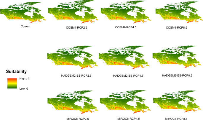
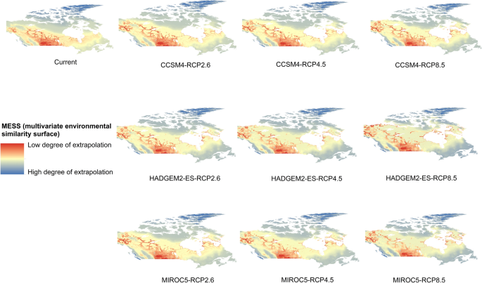
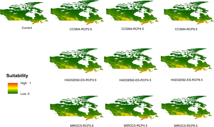
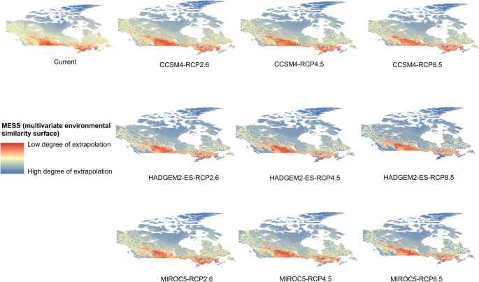
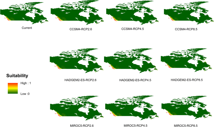
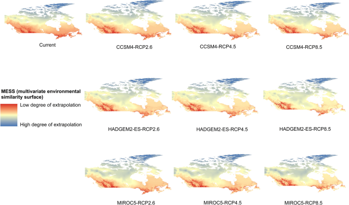
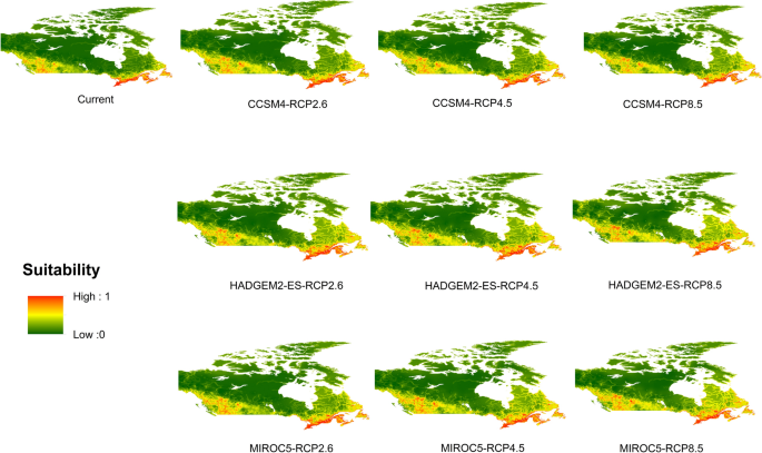
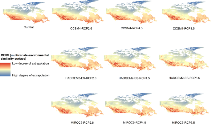
Potential distribution of selected FIS in current and future climate change scenarios along with MESS (multivariate environmental similarity surface) maps. For suitability maps, higher probability (red colors) represent areas suitable for FIS. Zero probability or lower probability (dark green) indicates areas less suitable. For MESS maps, increase in blue tone denotes increasing degree of extrapolation on at least one variable. Suitability predictions in those areas (blue) should be treated with high caution.
-
(a)
Asian gyspy moth
-
(b)
Asian longhoned beetle
-
(c)
Sudden oak death
-
(d)
Dutch elm disease


Appendix 3
See Fig. 8.

Predicted potential distribution of selected FIS on a global scale. Higher probability (red colors) represent areas suitable for FIS. Zero probability or lower probability (dark blue) indicates areas less suitable
Appendix 4: environmental response curves
See Fig. 9.


Relationships between environmental predictors and the probability of the presence of FIS: red curves show the mean response and blue margins are ± 1 SD calculated over 10 replicates
Appendix 5
Comparing dispersal limited to unlimited FIS dispersal projections under climate change conditions. Here numbers represents total number of cells colonized under each scenario.
(a) Asian gypsy moth
GCM/scenario | Infestation point-Vancouver port | Infestation point-Toronto port | Unlimited dispersal | ||||||
|---|---|---|---|---|---|---|---|---|---|
ccsm4 | hadgem2es | miroc5 | ccsm4 | hadgem2es | miroc5 | ccsm4 | hadgem2es | miroc5 | |
rcp26 | 3416 | 4143 | 5074 | 5393 | 5260 | 5499 | 19,142 | 19,509 | 19,265 |
rcp45 | 5262 | 4608 | 5115 | 5479 | 5532 | 5726 | 19,383 | 19,592 | 19,445 |
rcp85 | 5318 | 5473 | 5939 | 5619 | 5788 | 5843 | 19,548 | 19,770 | 19,599 |
(b) Asian longhorned beetle
GCM/scenario | Infestation point-Vancouver port | Infestation point-Toronto port | Unlimited dispersal | ||||||
|---|---|---|---|---|---|---|---|---|---|
ccsm4 | hadgem2es | miroc5 | ccsm4 | hadgem2es | miroc5 | ccsm4 | hadgem2es | miroc5 | |
rcp26 | 71 | 76 | 68 | 2482 | 2497 | 2446 | 7701 | 7366 | 7647 |
rcp45 | 75 | 82 | 72 | 2528 | 2539 | 2613 | 8117 | 7904 | 8116 |
rcp85 | 76 | 91 | 79 | 2567 | 2587 | 2663 | 8716 | 8510 | 8334 |
(c) Dutch elm disease
GCM/scenario | Infestation point-Toronto port | Unlimited dispersal | ||||
|---|---|---|---|---|---|---|
ccsm4 | hadgem2es | miroc5 | ccsm4 | hadgem2es | miroc5 | |
rcp26 | 1438 | 1379 | 1443 | 2051 | 2045 | 1992 |
rcp45 | 1538 | 1555 | 1524 | 2026 | 2061 | 2013 |
rcp85 | 1577 | 1616 | 1622 | 2039 | 2059 | 2040 |
(d) Sudden oak death
GCM/scenario | Infestation point-Vancouver port | Unlimited dispersal | ||||
|---|---|---|---|---|---|---|
ccsm4 | hadgem2es | miroc5 | ccsm4 | hadgem2es | miroc5 | |
rcp26 | 879 | 625 | 893 | 1166 | 977 | 1061 |
rcp45 | 606 | 650 | 848 | 1063 | 947 | 1097 |
rcp85 | 433 | 500 | 759 | 1033 | 911 | 1036 |
Appendix 6
FIS dispersal limited distributions under different climate change scenarios and two hypothesized infestation points-
AGM (Infestation point-Vancouver port)

Dispersal restricted future distribution of AGM under GCM-CCM4 and RCP 2.6, 4.5 and 8.5 climate change scenarios. Color gradient from blue to grey represents the first 10 years of the simulation time frame when colonization first occurred, the light grey to light yellow color gradient represents the next 10 years followed by orange and rose color gradients (years 2031–2050). Pink colored pixel indicates the hypothesized point of DED introduction (port of Toronto) while the green pixels represent suitable areas that were not colonized due to dispersal limitations and not reached by FIS during the time of simulation.

Dispersal restricted future distribution of AGM under GCM-HADGEM2ES and RCP 2.6, 4.5 and 8.5 climate change scenarios. Color gradient from blue to grey represents the first 10 years of the simulation time frame when colonization first occurred, the light grey to light yellow color gradient represents the next 10 years followed by orange and rose color gradients (years 2031–2050). Pink colored pixel indicates the hypothesized point of DED introduction (port of Toronto) while the green pixels represent suitable areas that were not colonized due to dispersal limitations and not reached by FIS during the time of simulation.

Dispersal restricted future distribution of AGM under GCM-MIROC5 and RCP 2.6, 4.5 and 8.5 climate change scenarios. Color gradient from blue to grey represents the first 10 years of the simulation time frame when colonization first occurred, the light grey to light yellow color gradient represents the next 10 years followed by orange and rose color gradients (years 2031–2050). Pink colored pixel indicates the hypothesized point of DED introduction (port of Toronto) while the green pixels represent suitable areas that were not colonized due to dispersal limitations and not reached by FIS during the time of simulation.
AGM (Introduction point-Toronto port)

Dispersal restricted future distribution of AGM under GCM-CCSM4 and RCP 2.6, 4.5 and 8.5 climate change scenarios. Color gradient from blue to grey represents the first 10 years of the simulation time frame when colonization first occurred, the light grey to light yellow color gradient represents the next 10 years followed by orange and rose color gradients (years 2031–2050). Pink colored pixel indicates the hypothesized point of DED introduction (port of Toronto) while the green pixels represent suitable areas that were not colonized due to dispersal limitations and not reached by FIS during the time of simulation.

Dispersal restricted future distribution of AGM under GCM-HADGEM2ES and RCP 2.6, 4.5 and 8.5 climate change scenarios. Color gradient from blue to grey represents the first 10 years of the simulation time frame when colonization first occurred, the light grey to light yellow color gradient represents the next 10 years followed by orange and rose color gradients (years 2031–2050). Pink colored pixel indicates the hypothesized point of DED introduction (port of Toronto) while the green pixels represent suitable areas that were not colonized due to dispersal limitations and not reached by FIS during the time of simulation.

Dispersal restricted future distribution of AGM under GCM-MIROC5 and RCP 2.6, 4.5 and 8.5 climate change scenarios. Color gradient from blue to grey represents the first 10 years of the simulation time frame when colonization first occurred, the light grey to light yellow color gradient represents the next 10 years followed by orange and rose color gradients (years 2031–2050). Pink colored pixel indicates the hypothesized point of DED introduction (port of Toronto) while the green pixels represent suitable areas that were not colonized due to dispersal limitations and not reached by FIS during the time of simulation.
ALB (Introduction point-Vancouver port)

Dispersal restricted future distribution of ALB under GCM-CCSM4 and RCP 2.6, 4.5 and 8.5 climate change scenarios. Color gradient from blue to grey represents the first 10 years of the simulation time frame when colonization first occurred, the light grey to light yellow color gradient represents the next 10 years followed by orange and rose color gradients (years 2031–2050). Pink colored pixel indicates the hypothesized point of DED introduction (port of Toronto) while the green pixels represent suitable areas that were not colonized due to dispersal limitations and not reached by FIS during the time of simulation.

Dispersal restricted future distribution of ALB under GCM-HADGEM2ES and RCP 2.6, 4.5 and 8.5 climate change scenarios. Color gradient from blue to grey represents the first 10 years of the simulation time frame when colonization first occurred, the light grey to light yellow color gradient represents the next 10 years followed by orange and rose color gradients (years 2031–2050). Pink colored pixel indicates the hypothesized point of DED introduction (port of Toronto) while the green pixels represent suitable areas that were not colonized due to dispersal limitations and not reached by FIS during the time of simulation.

Dispersal restricted future distribution of ALB under GCM-MIROC5 and RCP 2.6, 4.5 and 8.5 climate change scenarios. Color gradient from blue to grey represents the first 10 years of the simulation time frame when colonization first occurred, the light grey to light yellow color gradient represents the next 10 years followed by orange and rose color gradients (years 2031–2050). Pink colored pixel indicates the hypothesized point of DED introduction (port of Toronto) while the green pixels represent suitable areas that were not colonized due to dispersal limitations and not reached by FIS during the time of simulation.
ALB (Introduction point-Toronto port)

Dispersal restricted future distribution of ALB under GCM-CCSM4 and RCP 2.6, 4.5 and 8.5 climate change scenarios. Color gradient from blue to grey represents the first 10 years of the simulation time frame when colonization first occurred, the light grey to light yellow color gradient represents the next 10 years followed by orange and rose color gradients (years 2031–2050). Pink colored pixel indicates the hypothesized point of DED introduction (port of Toronto) while the green pixels represent suitable areas that were not colonized due to dispersal limitations and not reached by FIS during the time of simulation.

Dispersal restricted future distribution of ALB under GCM-HADGEM2ES and RCP 2.6, 4.5 and 8.5 climate change scenarios. Color gradient from blue to grey represents the first 10 years of the simulation time frame when colonization first occurred, the light grey to light yellow color gradient represents the next 10 years followed by orange and rose color gradients (years 2031–2050). Pink colored pixel indicates the hypothesized point of DED introduction (port of Toronto) while the green pixels represent suitable areas that were not colonized due to dispersal limitations and not reached by FIS during the time of simulation.

Dispersal restricted future distribution of ALB under GCM-MIROC5 and RCP 2.6, 4.5 and 8.5 climate change scenarios. Color gradient from blue to grey represents the first 10 years of the simulation time frame when colonization first occurred, the light grey to light yellow color gradient represents the next 10 years followed by orange and rose color gradients (years 2031–2050). Pink colored pixel indicates the hypothesized point of DED introduction (port of Toronto) while the green pixels represent suitable areas that were not colonized due to dispersal limitations and not reached by FIS during the time of simulation.
DED (Introduction point-Toronto port)

Dispersal restricted future distribution of DED under GCM-CCM4 and RCP 2.6, 4.5 and 8.5 climate change scenarios. Color gradient from blue to grey represents the first 10 years of the simulation time frame when colonization first occurred, the light grey to light yellow color gradient represents the next 10 years followed by orange and rose color gradients (years 2031–2050). Pink colored pixel indicates the hypothesized point of DED introduction (port of Toronto) while the green pixels represent suitable areas that were not colonized due to dispersal limitations and not reached by FIS during the time of simulation.

Dispersal restricted future distribution of DED under GCM-HADGEM2ES and RCP 2.6, 4.5 and 8.5 climate change scenarios. Color gradient from blue to grey represents the first 10 years of the simulation time frame when colonization first occurred, the light grey to light yellow color gradient represents the next 10 years followed by orange and rose color gradients (years 2031–2050). Pink colored pixel indicates the hypothesized point of DED introduction (port of Toronto) while the green pixels represent suitable areas that were not colonized due to dispersal limitations and not reached by FIS during the time of simulation.

Dispersal restricted future distribution of DED under GCM-MIROC5 and RCP 2.6, 4.5 and 8.5 climate change scenarios. Color gradient from blue to grey represents the first 10 years of the simulation time frame when colonization first occurred, the light grey to light yellow color gradient represents the next 10 years followed by orange and rose color gradients (years 2031–2050). Pink colored pixel indicates the hypothesized point of DED introduction (port of Toronto) while the green pixels represent suitable areas that were not colonized due to dispersal limitations and not reached by FIS during the time of simulation.
SOD (Introduction point-Vancouver port)

Dispersal restricted future distribution of SOD under GCM-CCM4 and RCP 2.6, 4.5 and 8.5 climate change scenarios. Color gradient from blue to grey represents the first 10 years of the simulation time frame when colonization first occurred, the light grey to light yellow color gradient represents the next 10 years followed by orange and rose color gradients (years 2031–2050). Pink colored pixel indicates the hypothesized point of DED introduction (port of Toronto) while the green pixels represent suitable areas that were not colonized due to dispersal limitations and not reached by FIS during the time of simulation.

Dispersal restricted future distribution of SOD under GCM-HADGEM2ES and RCP 2.6, 4.5 and 8.5 climate change scenarios. Color gradient from blue to grey represents the first 10 years of the simulation time frame when colonization first occurred, the light grey to light yellow color gradient represents the next 10 years followed by orange and rose color gradients (years 2031–2050). Pink colored pixel indicates the hypothesized point of DED introduction (port of Toronto) while the green pixels represent suitable areas that were not colonized due to dispersal limitations and not reached by FIS during the time of simulation.

Dispersal restricted future distribution of SOD under GCM-MIROC5 and RCP 2.6, 4.5 and 8.5 climate change scenarios. Color gradient from blue to grey represents the first 10 years of the simulation time frame when colonization first occurred, the light grey to light yellow color gradient represents the next 10 years followed by orange and rose color gradients (years 2031–2050). Pink colored pixel indicates the hypothesized point of DED introduction (port of Toronto) while the green pixels represent suitable areas that were not colonized due to dispersal limitations and not reached by FIS during the time of simulation.
Appendix 7
AGM life history parameters and associated references
AGM is a potent invader with more than 600 known hosts. AGM females are capable of flight and can lay eggs on human-made objects.
-
Generations per year
-
Univoltine—one generation per year (Elkinton and Liebhold 1990)
-
-
Dispersal
-
Dispersal distance
-
Frequent long distance dispersal flights (average less than 1 km to max range of 20–40 km) (Iwaizumi et al. 2010; Keena et al. 2008)
-
Russian females may fly distances up to 100 km and eastern Siberian females seen crossing mountain ranges in large groups during outbreaks (Rozhkov and Vasilyeva 1982)
-
Egg masses in Japanese cities found within 1 km of forests(Liebhold et al. 2008).
-
Average flight distance of 1 day old Chinese females in 8 h on flight mills was 5.65 km and maximum was 10.67 km (Yang et al. 2017)
-
-
Reproductive capacity
-
Producing an average of 600–1000 eggs per egg mass (USDA)
-
-
Distribution
-
Found throughout temperate Asia. Usually east of the Ural Mountains into Far East Russia, through most of Japan, China and Korea. It is not found east of the Himalayan range in India (USDA)
-
-
Critical temp.
-
AGM populations may struggle in regions experiencing longer periods of temperatures ≥ 30 °C and survival rate is highest between 15and 25 °C (Limbu et al. 2017).
-
ALB life history parameters and associated references
-
Sex ratio
-
Generations per year
-
Temperature dependent
-
Not strictly univoltine (1 year); may take multiple years to develop
-
(Keena and Moore 2010; Trotter and Keena 2016) (in Finland may take 10+ years)
-
(Straw et al. 2015)
-
3 years for Paddock Woods
-
-
(Kappel et al. 2017)
-
Do not use the Newtonian Cooling model to estimate within tree temps—may not accurately reflect temps within tree
-
But estimated that in northern states will take minimum 2–3 years to complete development, some areas up to 5–6 years
-
-
-
-
Dispersal distance
-
Frequent short distance dispersal flights (< 1.5 km)
-
(Javal et al. 2018)
-
-
Tendency to remain on and reinfest natal tree
-
(Haack et al. 2010)
-
-
Dispersal occurs when tree host quality deteriorates
-
(Sawyer 2011)
-
-
Rare long distance flights (< 1.5 km)
-
Human mediated transport likely more significant at farther distances
-
(Fournier and Turgeon 2017)
-
-
-
~ 10 km (modeled and based on graph)
-
(Trotter et al. 2019)
-
-
Longest single sustained flight on flight mill = 4006 m; median = 247.6 m
-
(Javal et al. 2018)
-
-
Lifetime dispersal for a female = 14,060 m; median = 3964 m
-
(Javal et al. 2018)
-
-
-
Spread rates
-
Probability to disperse
-
Critical temps
-
Habitat preferences
DED biology and vector life history
DED is vectored by several species of bark beetle: Hylurgopinus rufipes (native), Scolytus multistriatus (introduced-Europe), and Scolytpus schevyrewi (introduced-Asia).
-
Surprising lack of dispersal information for above three species
-
(Harwood et al. 2011)
-
-
Dispersal kernel
-
(Harwood et al., 2011)
-
DED vectors
-
Negative exponential kernel of 20 km (15–40 km)
-
Experts estimate max dispersal = 12.88 km
-
Most dispersal within 500 m of host
-
Median dispersal distance of 150 m for a negative square power law function for incorporating radial dispersal
-
Probability of 0.002 for dispersal > 12.88 km
-
Combined beetle and firewood kernel of 3:1 beetle:firewood movement gives a reasonable pattern of spread in early stages of epidemic
-
-
-
-
History of DED in UK
-
(Tomlinson and Potter 2010)
-
-
Review of factors influencing flight in bark beetles (Jones et al. 2019)
-
Bark beetles (= Scolytinae) contain vectors of DED
-
Flight capacity versus dispersal—distinct
-
Capacity = physiological ability to fly
-
Dispersal = capacity + imapct of external factors (e.g. environment)
-
Long distance dispercal characterized by above canopy flight carried by wind (e.g. Mountain pine beetle dispersal over Rocky Mountains; 30–100 km/day via wind)
-
-
-
Dispersal distance
-
mean for beetles ranges from 500 m to 6 km; max distances can be > 25 km, but this is a long thin tail, bulk of the pop is short distance
-
-
Fat-tailed dispersal kernel needed to capture potential for bark beetles to disperse long distances
-
Min temp for flight initiation in bark beetles range from 10.6C–21C; mean = 15.6C
-
Dispersal distance
SOD biology and vector life history parameters and associated references
There are no known vectors of SOD other than humans but any organism that can move soil is potentially a vector of SOD.(Grünwald et al. 2012, 2019; Kliejunas 2010; Rizzo et al. 2005)
-
Dispersal
-
Long range spread of disease through sporangia and chlamydospores, chlamydospores can survive for a week at a constant temperature of 55 °C.
-
Natural dispersal of SOD is by movement of plant material, waterborne and soilborne chlamydospores, and by waterborne, soilborne and wind-blown rain containing sporangia (Rizzo and Garbelotto 2003; Rizzo et al. 2005; Grünwald et al. 2019)
-
-
Dispersal distance
-
Splash dispersal-propagules can travel up to 60 cm above infested surfaces (Kuske 1983).
-
Local spread < 1 km (ecological (Condeso et al. 2007; Ellis et al. 2010) and genetic (Mascheretti et al. 2008, 2009))
-
Most inoculum remains within 10 m of the host (Davidson et al. 2005)
-
Maximum dispersal distance < 8 km during rare storm events (apsnet.org).
-
Number of trees infected was higher on public lands that were open to recreation than on adjacent lands lacking public access and higher human population densities within 50 km increased chances of fungal infection (Cushman et al. 2008).
-
-
Effects of temperature and moisture on growth and sporulation
-
Fungal growth occurs 10–31 °C (Tooley et al. 2009)
-
Exposure to temperatures over 30 °C decreases survival and a few minutes at 40 °C kills the fungus (Browning et al. 2008)
-
Sporangia production occurs over the temperature range of 16–22 °C (Englander et al. 2006)
-
A dew period of as little as 1 h was enough for fungal development but moisture for 24–48 h is required for maximal disease development in the laboratory (Tooley et al. 2009)
-
Most clonal hyphal colonies can survive 24 h exposure to − 5 C and some can withstand − 25 C for 24 h. (Browning et al. 2008).
-
-
Distribution
-
SOD is distributed only in Europe and parts of North America, with three identified clonal lineages (EU1, NA1 and NA2), named for the continent where they were first found, followed by a number indicating the order of discovery (Grünwald et al. 2009)
-
-
Habitat
Appendix 8 (MigClim: Calibration of PDisp)-based on source (Engler and Guisan 2009)
PDisp, is the colonization probability of a pixel given its distance from a source pixel. To calibrate PDisp we defined a dispersal kernel used to model regular seed dispersal. The kernel was based on the following negative exponential seed dispersal probability distribution function (Eq. 1).
Further simplified in more conventional simple negative exponential form (Eq. 2)
where Pseed is the probability of a seed reaching distance x ≥ pixelsize, pixelsize is the one-dimensional size of a pixel, DispDist is the dispersal distance reached by the proportion k of the seeds.
Since the surface composed of pixels located at distance j from a source cell increases with distance from that source cell, the probability of a pixel to receive a seed is computed as (Eq. 3)
where Surfacej is the number of pixels covered by all pixels belonging to a same distance class. Assuming that the distribution of successful seeds (i.e. seeds leading a pixel to become colonized) is proportional to the overall distribution of seeds (Pseed), PDisp is computed as (Eq. 4):
where PDisp is the probability of colonisation for a target pixel with distance j from a source pixel and Successful Seeds the number of successful seeds produced by a fully mature source pixel.
Rights and permissions
About this article

Cite this article
Srivastava, V., Roe, A.D., Keena, M.A. et al. Oh the places they’ll go: improving species distribution modelling for invasive forest pests in an uncertain world. Biol Invasions 23, 297–349 (2021). https://doi.org/10.1007/s10530-020-02372-9
Received:
Accepted:
Published:
Issue Date:
DOI: https://doi.org/10.1007/s10530-020-02372-9