


Abstract
We present the details of the photometric and astrometric calibration of the Pan-STARRS1 3π Survey. The photometric goals were to reduce the systematic effects introduced by the camera and detectors, and to place all of the observations onto a photometric system with consistent zero-points over the entire area surveyed, the ≈30,000 deg2 north of δ = −30°. Using external comparisons, we demonstrate that the resulting photometric system is consistent across the sky to between 7 and 12.4 mmag depending on the filter. For bright stars, the systematic error floor for individual measurements is (σg, σr, σi, σz, σy) = (14, 14, 15, 15, 18) mmag. The astrometric calibration compensates for similar systematic effects so that positions, proper motions, and parallaxes are reliable as well. The bright-star systematic error floor for individual astrometric measurements is 16 mas. The Pan-STARRS Data Release 2 (DR2) astrometric system is tied to the Gaia DR1 coordinate frame with a systematic uncertainty of ∼5 mas.
Export citation and abstract BibTeX RIS
1. Introduction
From 2010 May through 2014 March, the Pan-STARRS Science Consortium used the 1.8 m Pan-STARRS1 telescope to perform a set of wide-field science surveys. These surveys are designed to address a range of science goals, including the search for hazardous asteroids, the study of the formation and architecture of the Milky Way galaxy, and the search for Type Ia supernovae to measure the history of the expansion of the universe. The majority of the time (56%) was spent on surveying the three-quarters of the sky north of −30° decl. with  ,
,  ,
,  ,
,  , and
, and  filters in the so-called 3π Survey. Another ∼25% of the time was concentrated on repeated deep observations of 10 specific fields in the Medium-Deep Survey. The rest of the time was used for several other surveys, including a search for potentially hazardous asteroids in our solar system. The details of the telescope, surveys, and resulting science publications are described by Chambers et al. (2016).
The wide-field Pan-STARRS1 telescope consists of a 1.8 m diameter f/4.4 primary mirror with an 0.9 m secondary, producing a 33 field of view (Hodapp et al. 2004). The optical design yields low distortion and minimal vignetting even at the edges of the illuminated region. The optics, in combination with the natural seeing, result in generally good image quality: the median image quality for the 3π Survey is FWHM = (131, 119, 111, 107, 102) for ( ,
,  ,
,  ,
,  ,
,  ), with a floor of ∼07. The Pan-STARRS1 camera (Tonry & Onaka 2009) is a mosaic of 60 edge-abutted 4800 × 4800 pixel back-illuminated CCID58 Orthogonal Transfer Arrays manufactured by Lincoln Laboratory (Tonry et al. 2006, 2008). The CCDs have 10 μm pixels subtending 0258 and are 70 μm thick. The detectors are read out using a StarGrasp CCD controller, with a readout time of 7 s for a full unbinned image (Onaka et al. 2008). The active, usable pixels cover ∼80% of the field of view. Figure 1 illustrates the physical layout of the devices in the camera with respect to the parity of the sky.

Figure 1. Diagram illustrating the layout of OTA devices in GPC1. The blue dots mark the locations of the amplifiers for xy00 cells in each chip. When cells are mosaicked to a single pixel grid, the pixel in this corner is at chip coordinate (0, 0). The figure illustrates the orientation of the OTA devices relative to the parity of the sky. An exposure taken with north at the top of the field of view will have east to the left when the OTA devices are mosaicked as shown. Note that the devices OTA0Y—OTA3Y are rotated by 180° relative to the other half of the camera. The labeling of the nonexistent corner OTAs is provided to orient the focal plane.
Download figure:
Standard image High-resolution imageNightly observations are conducted remotely from the Advanced Technology Research Center in Kula, the main facility of the University of Hawaii's Institute for Astronomy operations on Maui. During the Pan-STARRS1 Science Survey, images obtained by the Pan-STARRS1 system were stored first on computers at the summit, then copied with low latency via internet to the dedicated data analysis cluster located at the Maui High Performance Computer Center in Kihei, Maui.
Pan-STARRS produced its first large-scale public data release, Data Release 1 (DR1) on 16 December 2016. DR1 contains the results of the third full reduction of the Pan-STARRS 3π Survey archival data, identified as PV3. Previous reductions (PV0, PV1, and PV2; see Magnier et al. 2020a) were used internally for pipeline optimization and the development of the initial photometric and astrometric reference catalog. The products from these reductions were not publicly released but have been used to produce a wide range of scientific papers from the Pan-STARRS1 Science Consortium members (Chambers et al. 2016). DR1 contained only average information resulting from the many individual images obtained by the 3π Survey observations. A second data release, DR2, was made available on 2019 January 28. DR2 provides measurements from all of the individual exposures and include an improved calibration of the PV3 processing of that data set.
This is the fifth in a series of seven papers describing the Pan-STARRS1 Surveys, the data reduction techniques and the resulting data products. This paper (Paper V) describes the final calibration process and the resulting photometric and astrometric quality.
Chambers et al. (2016, Paper I) provides an overview of the Pan-STARRS System, the design and execution of the Surveys, the resulting image and catalog data products, a discussion of the overall data quality and basic characteristics, and a brief summary of important results.
Magnier et al. (2020a, Paper II) describes how the various data processing stages are organized and implemented in the Image Processing Pipeline (IPP), including details of the the processing database which is a critical element in the IPP infrastructure .
Waters et al. (2020, Paper III) describes the details of the pixel processing algorithms, including detrending, warping, and adding (to create stacked images) and subtracting (to create difference images), and the resulting image products and their properties.
Magnier et al. (2020b, Paper IV) describes the details of the source detection and photometry, including point-spread-function (PSF) and extended source fitting models, and the techniques for "forced" photometry measurements.
Flewelling et al. (2020, Paper VI) describes the details of the resulting catalog data and its organization in the Pan-STARRS database.
M. Huber et al. (2020, in preparation, Paper VII) describes the Medium-Deep Survey in detail, including the unique issues and data products specific to that survey. The Medium-Deep Survey is not part of DR1 or DR2 and will be made available in a future data release.
The Pan-STARRS1 filters and photometric system have already been described in detail in Tonry et al. (2012).
2. Pan-STARRS1 Data Analysis
Images obtained by Pan-STARRS1 are automatically processed in real time by the Pan-STARRS1 IPP (see Paper II). Real-time analysis goals are aimed at feeding the discovery pipelines of the asteroid search and supernova search teams. The data obtained for the Pan-STARRS1 Science Survey have also been used in three additional complete reprocessing of the data: Processing Versions 1, 2, and 3 (PV1, PV2, and PV3). The real-time processing of the data is considered "PV0." Except as otherwise noted, this article describes the calibration of the PV3 analysis of the data. Between DR1 and DR2, improvements were made to the calibration of both the photometry and astrometry, as described in this article.
The pipeline data processing steps are described in detail in Papers II, III, and IV. In summary, individual images are detrended: nonlinearity and bias corrections are applied, a dark current model is subtracted, and flat-field corrections are applied. The  -band images are also corrected for fringing: a master fringe pattern is scaled to match the observed fringing and subtracted. Mask and variance image arrays are generated with the detrend analysis and carried forward at each stage of the IPP processing. Source detection and photometry are performed for each chip independently. As discussed below, preliminary astrometric and photometric calibrations are performed for all chips in a single exposure in a single analysis. We refer to these measurements as the "chip" photometry and astrometry products.
Chip images are geometrically transformed based on the astrometric solution into a set of predefined pixel grids covering the sky, called skycells. These transformed images are called the warp images. Sets of warps for a given part of the sky and in the same filter may be added together to generate deeper "stack" images. PSF matched difference images are generated from combinations of warps and stacks; the details of the difference images and their calibration are outside of the scope of this article.
Astronomical objects are detected and characterized in the stack images. The details of the analysis of the sources in the stack images are discussed in Paper IV, but in brief, these include PSF photometry, along with a range of measurements driven by the goals of understanding the galaxies in the images. Because of the significant mask fraction of the GPC1 focal plane and the varying image quality both within and between exposures, the effective PSF of the Pan-STARRS1 Survey (PS1) stack images (often including more than 10 input exposures taken in different conditions) is highly variable. The PSF varies significantly on scales as small as a few to tens of pixels, making accurate PSF modeling essentially infeasible. The PSF photometry of sources in the stack images is thus degraded significantly compared to the quality of the photometry measured for the individual chip images.
To recover most of the photometric quality of the individual chip images while also exploiting the depth afforded by the stacks, the PV3 analysis makes use of forced photometry on the individual warp images. PSF photometry is measured on the warp images for all sources that are detected in the stack images images. The positions determined in the stack images are used in the warp images, but the PSF model is determined for each warp independently based on brighter stars in the warp image. The only free parameter for each object is the flux, which may be insignificant or even negative for sources that are near the faint limit of the stack detections. When the fluxes from the individual warp images are averaged, a reliable measurement of the faint source flux is determined. The details of this analysis are described in detail in Paper IV.
The data products from the chip photometry, stack photometry, and forced-warp photometry analysis stages are ingested into the internal calibration database called the Desktop Virtual Observatory, or DVO (see Section 4 in Paper II) and used for photometric and astrometric calibrations. In this article, we discuss the photometric calibration of the individual exposures, the stacks, and the warp images. We also discuss the astrometric calibration of the individual exposures and the stack images.
3. Pipeline Calibration
3.1. Overview
As images are processed by the data analysis system, every exposure is calibrated individually with respect to a photometric and astrometric reference database. The goal of this calibration step is to generate a preliminary astrometric calibration, to be used by the warping analysis to determine the geometric transformation of the pixels, and a preliminary photometric transformation, to be used by the stacking analysis to ensure the warps are combined using consistent flux units.
The program used for the pipeline calibration, psastro, loads the measurements of the chip detections from their individual output catalog files. It uses the header information populated at the telescope to determine an initial astrometric calibration guess based on the position of the telescope boresite R.A., decl., and position angle as reported by the telescope & camera subsystems. Using the initial guess, psastro loads astrometric and photometric data from the reference database.
3.2. Reference Catalogs
During the course of the PS1SC Survey, several reference databases have been used. For the first 20 months of the survey, psastro used a reference catalog with synthetic PS1  ,
,  ,
,  ,
,  ,
,  photometry generated by the Pan-STARRS IPP team based on combined photometry from Tycho (B, V), USNO (red, blue, IR Monet et al. 2003), and Two Micron All Sky Survey (2MASS) J, H, K (Skrutskie et al. 2006). The astrometry in the database was from 2MASS (Skrutskie et al. 2006). After 2012 May, a reference catalog generated from internal recalibration of the PV0 analysis of PS1 photometry and astrometry was used for the reference catalog.
Coordinates and calibrated magnitudes of stars from the reference database are loaded by psastro. A model for the positions of the 60 chips in the focal plane is used to determine the expected astrometry for each chip based on the boresite coordinates and position angle reported by the header. Reference stars are selected from the full field of view of the GPC1 camera, padded by an additional 25% to ensure a match can be determined even in the presence of substantial errors in the boresite coordinates. It is important to choose an appropriate set of reference stars: if too few are selected, the chance of finding a match between the reference and observed stars is diminished. In addition, because stars are loaded in brightness order, a selection that is too small is likely to contain only stars that are saturated in the GPC1 images. On the other hand, if too many reference stars are chosen, there is a higher chance of a false-positive match, especially as many of the reference stars may not be detected in the GPC1 image. The selection of the reference stars includes a limit on the brightest and faintest magnitudes of the stars selected.
The astrometric analysis is necessarily performed first; after the astrometry is determined, an automatic byproduct is a reliable match between reference and observed stars, allowing a comparison of the magnitudes to determine the photometric calibration.
3.3. Astrometric Models
Three somewhat distinct astrometric models are employed within the IPP at different stages. The simplest model is defined independently for each chip: a simple TAN projection as described by Calabretta & Greisen (2002) is used to relate sky coordinates to a Cartesian tangent-plane coordinate system. A pair of low-order polynomials is used to relate the chip pixel coordinates to this tangent-plane coordinate system. The transforming polynomials are of the form:


where P, Q are the tangent-plane coordinates, X, Y are the coordinates on the 60 GPC1 chips, and  are the polynomial coefficients for each order i, j. In the psastro analysis, i + j < = Norder, where the order of the fit, Norder, may be 1 to 3, under the restriction that sufficient stars are needed to constrain the order.
A second form of astrometry model, which yields a somewhat higher accuracy, consists of a set of connected solutions for all chips in a single exposure. This model also uses a TAN projection to relate the sky coordinates to a locally Cartesian tangent-plane coordinate system. A set of polynomials is then used to relate the tangent-plane coordinates to a "focal plane" coordinate system, L, M:


This set of polynomials accounts for effects such as optical distortion in the camera and distortions due to changing atmospheric refraction across the field of the camera. Because these effects are smooth across the field of the camera, a single pair of polynomials can be used for each exposure. As in the chip analysis above, the psastro code restricts the exponents with the rule i + j < = Norder, where the order of the fit, Norder, may be 1 to 3, under the restriction that sufficient stars are needed to constrain the order. For each chip, a second set of polynomials describes the transformation from the chip coordinate systems to the focal coordinate system:


A third form of the astrometry model is used in the context of the calibration determined within the DVO database system. We retain the two levels of transformations (chip  focal plane
  tangent plane), but the relationship between the chip and focal plane is represented by only the linear terms in the polynomial, supplemented by a coarse grid of displacements, δL, δM, sampled across the coordinate range of the chip. This displacement grid may have a resolution of up to 6 × 6 samples across the chip. The displacement for a specific chip coordinate value is determined via bilinear interpolation between the nearest sample points. Thus, the chip to focal-plane transformation may be written as


These high-order transformations are required for the individual chips to follow small-scale distortions due to the optics (stable from exposure to exposure) as well as the atmosphere (changes from over time). The spatial scale on which the astrometric deviations due to the atmosphere are varying is related to the isoplanatic patch size. We note that, in the typical conditions at the Pan-STARRS1 site, if the seeing is due to low-lying atmospheric layers, the isoplanatic patch scale will be at most a few arcminutes (Beckers 1988) and smaller when the seeing comes from higher altitudes.
We also note that, in our detailed astrometric analysis within the database system, we perform an initial correction for several systematic effects, including the color-dependent correction due to differential chromatic refraction. The corrected chip positions are the inputs to the equations above (see Section 6.1).
3.4. Cross-correlation Search
The first step of the analysis is to attempt to find the match between the reference stars and the detected objects. psastro uses 2D cross-correlation to search for the match. The guess astrometry calibration is used to define a predicted set of Xref, Yref values for the reference catalog stars. For all possible pairs between the two lists, the values of


are generated. The collection of ΔX, ΔY values are collected in a 2D histogram with a sampling of 50 pixels, and the peak pixel is identified. If the astrometry guess were perfect, this peak pixel would be expected to lie at (0, 0) and contain all of the matched stars. However, the astrometric guess may be wrong in several ways. An error in the constant term above,  shifts the peak to another pixel, from which
  can easily be determined. An error in the plate scale or a rotation will smear out the peak pixel potentially across many pixels in the 2D histogram.
To find a good match in the face of plate scale and rotation errors, the cross-correlation analysis above is performed for a series of trials in which the scale and rotation are perturbed from the nominal value by a small amount. For each trial, the peak pixel is found and a figure of merit is measured. The figure of merit is defined as  , where
  is the second moment of ΔX, Y for the star pairs associated with the peak pixel, and Np
is the number of star pairs in the peak. This figure of merit is thus most sensitive to a narrow distribution with many matched pairs. For the PS1 exposures, rotation offsets of (−10, −05, 00, 05, 10) and plate scales of (+1%, 0, −1%) of the nominal plate scale are tested. The best match among these 15 cross-correlation tests is selected and used to generate a better astrometry guess for the chip.
is the second moment of ΔX, Y for the star pairs associated with the peak pixel, and Np
is the number of star pairs in the peak. This figure of merit is thus most sensitive to a narrow distribution with many matched pairs. For the PS1 exposures, rotation offsets of (−10, −05, 00, 05, 10) and plate scales of (+1%, 0, −1%) of the nominal plate scale are tested. The best match among these 15 cross-correlation tests is selected and used to generate a better astrometry guess for the chip.
3.5. Pipeline Astrometric Calibration
The astrometry solution from the cross-correlation step above is again used to select matches between the reference stars and observed stars in the image. The matching radius starts off quite large, and a series of fits is performed to generate the transformation between chip and tangent-plane coordinates. Three clipping iterations are performed, with outliers >3σ rejected on each pass, where here σ is determined from the distribution of the residuals in each dimension (X, Y) independently. After each fit cycle, the matches are redetermined using a smaller radius and the fit retried.
The astrometry solutions from the independent chip fits are used to generate a single model for the camera-wide distortion terms. The goal is to determine the two-stage fit (chip  focal plane
  tangent plane). There are a number of degenerate terms between these two levels of transformation, most obviously between the parameters that define the constant offset from chip to focal plane (
 ) and those that define the offset from focal plane to tangent plane (
 ). We limit (
 ) to be 0, 0 to remove this degeneracy.
The initial fit of the astrometry for each chip follows the distortion introduced by the camera: the apparent plate scale for each chip is the combination of the plate scale at the optical axis of the camera, modified by the local average distortion. To isolate the effect of distortion, we choose a single common plate scale for the set of chips and redefine the chip  sky calibrations as a set of chip
  focal-plane transformations using that common pixel scale. We can now compare the observed focal-plane coordinates, derived from the chip coordinates, and the tangent-plane coordinates, derived from the projection of the reference coordinates. One caveat is that the chip reference coordinates are also degenerate with the fitted distortion. To avoid being sensitive to the exact positions of the chips at this stage, we measure the local gradient between the focal-plane and tangent-plane coordinate systems. We then fit the gradient with a polynomial of order 1 less than the polynomial desired for the distortion fit. The coefficients of the gradient fit are then used to determine the coefficients for the polynomials representing the distortion.
Once the common distortion coming from the optics and atmosphere have been modeled, psastro determines polynomial transformations from the 60 chips to the focal-plane coordinate system. At this stage, five iterations of the chip fits are performed. Before each iteration, the reference stars and detected objects are matched using the current best set of transformations. These fits start with low order (1) and large matching radius. As the iterations proceed, the radius is reduced and the order is allowed to increase, up to third order for the final iterations.
3.6. Pipeline Photometric Calibration
After the astrometric calibration is determined, the photometric calibration is performed by psastro. When the reference stars are loaded, the apparent magnitude in the filter of interest is also loaded. Stars for which the reference magnitude is brighter than ( ,
,  ,
,  ,
,  ,
,  ) = (19, 19, 18.5, 18.5, 17.5) are used to determine the zero-points by comparison with the instrumental magnitudes. For the PV3 analysis, an outlier-rejecting median is used to measure the zero-point. For early versions of the pipeline analysis, when the reference catalog used synthetic magnitudes, it was necessary to search for the blue edge of the distribution: the synthetic magnitude poorly predicted the magnitudes of stars in the presence of significant extinction or for the very red stars, making the blue edge somewhat more reliable as a reference than the mean. Once the calibration was based on a reference catalog generated from Pan-STARRS1 photometry, this methods was no longer needed. Note that we do not fit for the airmass slope in this analysis. The nominal airmass slope is used for each filter; any deviation from the nominal value is effectively folded into the observed zero-point. The zero-point may be measured separately for each chip or as a single value for the entire exposure; the latter option was used for the PV3 analysis.
3.7. Outputs
The calibrations determined by psastro are saved as part of the header information in the output FITS tables. For each exposure, a single multi-extension FITS table is written. In these files, the measurements from each chip are written as a separate FITS table. A second FITS extension for each chip is used to store the header information from the original chip image. The original chip header is modified so that the extension corresponds to an image with no pixel data: NAXISis set to 0, even though NAXIS1 and NAXIS2 are retained with the original dimensions of the chip. A pixel-less primary header unit (PHU) is generated with a summary of some of the important and common chip-level keywords (e.g., DATE-OBS). The astrometric transformation information for each chip is saved in the corresponding header using standard (and some nonstandard) WCS keywords. For the two-level astrometric model, the PHU header carries the astrometric transformation related to the projection and the camera-wide distortions. Photometric calibrations are written as a set of keywords to individual chip headers and, if the calibration is performed at the exposure level, to the PHU. The photometry calibration keywords are:
- 1.ZPT_REF : the nominal zero-point for this filter
- 2.ZPT_OBS : the measured zero-point for this chip/exposure
- 3.ZPT_ERR : the standard deviation of ZPT_OBS
- 4.ZPT_NREF : the number of stars used to measure ZPT_OBS
- 5.ZPT_MIN : minimum reference magnitude included in analysis
- 6.ZPT_MAX : maximum reference magnitude included in analysis
The keyword ZPT_OBS is used to set the initial zero-point when the data from the exposure are loaded into the DVO database.
4. Calibration Database
Data from the GPC1 chip images, the stack images, and the warp images are loaded into the DVO calibration database using the real-time analysis astrometric calibration to guide the association of detections into objects. After the full PV3 DVO database was constructed, including all of the chip, stack, and warp detections, several external catalogs were merged into the database. First, the complete 2MASS PSC was loaded into a stand-alone DVO database, which was then merged into the PV3 master database. Next, the DVO database of synthetic photometry in the PS1 bands (see Section 3.2) was merged in. Next, the full Tycho database was added, followed by the AllWISE database. After the Gaia DR1 in August 2016 (Gaia Collaboration et al. 2016), we generated a DVO database of the Gaia positional and photometric information and merged that into the master PV3 3π DVO database.
The master DVO database is used to perform the full photometric and astrometric calibration of the PS1 data. During these analysis steps, a wide variety of conditions are noted for individual measurements, for the objects (either as a whole or for specific filters) and for the images. A set of bit-valued flags is used in the database to record these conditions. Table 1 lists the flags specific to individual measurements. These values are stored in the DVO database in the field Measure.dbFlags and exposed in the public database (PSPS; Paper VI) in the fields Detection.infoFlag3, StackObjectThin.XinfoFlag3 (where X is one of grizy), and ForcedWarpMeasurement.FinfoFlag3. Table 2 lists the flags that are set for each filter for individual objects in the database. These values are recorded in the DVO database field SecFilt.flags and are exposed in PSPS in the fields MeanObject.XFlags and StackObjectThin.XinfoFlag4, where X in both cases is one of grizy. Table 3 lists the flags specific to an object as a whole. These values are stored in the DVO database field Average.flags and are exposed in PSPS in the field MeanObject.objInfoFlag. Table 4 lists the flags raised for images. These flags are stored in the DVO database field Image.flags and are exposed in PSPS in the field ImageMeta.qaFlags. The types of conditions that are recorded by these bits range from information about the presence of external measurements (e.g., 2MASS or WISE) to determinations of good- or bad-quality measurements for astrometry or photometry. In the sections below, the flag values in these tables are described where appropriate. Note that some of the listed bits are either ephemeral (used internal to specific programs) or are not relevant to the current DR2 analysis and reserved for future use.
Table 1. Per-measurement Flag Bit Values
| Bit Name | Bit Value | Description |
|---|---|---|
| ID_MEAS_NOCAL | 0x00000001 | detection ignored for this analysis (photcode, time range)—internal only |
| ID_MEAS_POOR_PHOTOM | 0x00000002 | detection is photometry outlier (not used for PV3) |
| ID_MEAS_SKIP_PHOTOM | 0x00000004 | detection was ignored for photometry measurement (not used for PV3) |
| ID_MEAS_AREA | 0x00000008 | detection near image edge (not used for PV3) |
| ID_MEAS_POOR_ASTROM | 0x00000010 | detection is astrometry outlier |
| ID_MEAS_SKIP_ASTROM | 0x00000020 | detection was not used for image calibration (not reported for PV3) |
| ID_MEAS_USED_OBJ | 0x00000040 | detection was used during update objects |
| ID_MEAS_USED_CHIP | 0x00000080 | detection was used during update chips (not saved for PV3) |
| ID_MEAS_BLEND_MEAS | 0x00000100 | detection is within the radius of multiple objects (not used for PV3) |
| ID_MEAS_BLEND_OBJ | 0x00000200 | multiple detections within the radius of object (not used for PV3) |
| ID_MEAS_WARP_USED | 0x00000400 | measurement used to find mean warp photometry |
| ID_MEAS_UNMASKED_ASTRO | 0x00000800 | measurement was not masked in final astrometry fit |
| ID_MEAS_BLEND_MEAS_X | 0x00001000 | detection is within the radius of multiple objects across catalogs (not used for PV3) |
| ID_MEAS_ARTIFACT | 0x00002000 | detection is thought to be non-astronomical (not used for PV3) |
| ID_MEAS_SYNTH_MAG | 0x00004000 | magnitude is synthetic (not used for DR2) |
| ID_MEAS_PHOTOM_UBERCAL | 0x00008000 | externally supplied zero-point from ubercal analysis |
| ID_MEAS_STACK_PRIMARY | 0x00010000 | this stack measurement is in the primary skycell |
| ID_MEAS_STACK_PHOT_SRC | 0x00020000 | this measurement supplied the stack photometry |
| ID_MEAS_ICRF_QSO | 0x00040000 | this measurement is an ICRF reference position (not used for PV3) |
| ID_MEAS_IMAGE_EPOCH | 0x00080000 | this measurement is registered to the image epoch (not used for PV3) |
| ID_MEAS_PHOTOM_PSF | 0x00100000 | this measurement is used for the mean PSF mag |
| ID_MEAS_PHOTOM_APER | 0x00200000 | this measurement is used for the mean ap mag |
| ID_MEAS_PHOTOM_KRON | 0x00400000 | this measurement is used for the mean Kron mag |
| ID_MEAS_MASKED_PSF | 0x01000000 | this measurement is masked based on IRLS weights for mean PSF mag |
| ID_MEAS_MASKED_APER | 0x02000000 | this measurement is masked based on IRLS weights for mean ap mag |
| ID_MEAS_MASKED_KRON | 0x04000000 | this measurement is masked based on IRLS weights for mean Kron mag |
| ID_MEAS_OBJECT_HAS_2MASS | 0x10000000 | measurement comes from an object with 2MASS data |
| ID_MEAS_OBJECT_HAS_GAIA | 0x20000000 | measurement comes from an object with Gaia data |
| ID_MEAS_OBJECT_HAS_TYCHO | 0x40000000 | measurement comes from an object with Tycho data |
| These DVO flags correspond to PSPS flags DetectionFlags3 (Paper VI, Table 18), but without the leading ID_MEAS_. | ||
Download table as: ASCIITypeset image
Table 2. Relphot Per-filter Info Flag Bit Values
| Bit Name | Bit Value | Description |
|---|---|---|
| ID_SECF_STAR_FEW | 0x00000001 | Used within relphot: skip star (not reported for PV3) |
| ID_SECF_STAR_POOR | 0x00000002 | Used within relphot: skip star (not reported for PV3) |
| ID_SECF_USE_SYNTH | 0x00000004 | Synthetic photometry used in average measurement (not used in PV3) |
| ID_SECF_USE_UBERCAL | 0x00000008 | Ubercal photometry used in average measurement |
| ID_SECF_HAS_PS1 | 0x00000010 | PS1 photometry used in average measurement |
| ID_SECF_HAS_PS1_STACK | 0x00000020 | PS1 stack photometry exists |
| ID_SECF_HAS_TYCHO | 0x00000040 | Tycho photometry used for synth mags (not used in PV3) |
| ID_SECF_FIX_SYNTH | 0x00000080 | Synth mags repaired with zpt map (not used in PV3) |
| ID_SECF_RANK_0 | 0x00000100 | Average magnitude uses rank 0 values |
| ID_SECF_RANK_1 | 0x00000200 | Average magnitude uses rank 1 values |
| ID_SECF_RANK_2 | 0x00000400 | Average magnitude uses rank 2 values |
| ID_SECF_RANK_3 | 0x00000800 | Average magnitude uses rank 3 values |
| ID_SECF_RANK_4 | 0x00001000 | Average magnitude uses rank 4 values |
| ID_SECF_OBJ_EXT_PSPS | 0x00002000 | In PSPS ID_SECF_OBJ_EXT is saved here so it fits within 16 bits |
| ID_SECF_STACK_PRIMARY | 0x00004000 | PS1 stack photometry includes a primary skycell |
| ID_SECF_STACK_BESTDET | 0x00008000 | PS1 stack best measurement is a detection (not forced) |
| ID_SECF_STACK_PRIMDET | 0x00010000 | PS1 stack primary measurement is a detection (not forced) |
| ID_SECF_STACK_PRIMARY_MULTIPLE | 0x00020000 | PS1 stack object has multiple primary measurements |
| ID_SECF_HAS_SDSS | 0x00100000 | This photcode has SDSS photometry (not used for PV3) |
| ID_SECF_HAS_HSC | 0x00200000 | This photcode has HSC photometry (not used for PV3) |
| ID_SECF_HAS_CFH | 0x00400000 | This photcode has CFH photometry (not used for PV3) |
| ID_SECF_HAS_DES | 0x00800000 | This photcode has DES photometry(not used for PV3) |
| ID_SECF_OBJ_EXT | 0x01000000 | Extended in this band |
| These DVO flags correspond to PSPS flags ObjectFilterFlags (PaperVI, Table 13), but without the leading ID_. | ||
Download table as: ASCIITypeset image
Table 3. Per-object Flag Bit Values
| Bit Name | Bit Value | Description |
|---|---|---|
| ID_OBJ_FEW | 0x00000001 | used within relphot: skip star (not reported for PV3) |
| ID_OBJ_POOR | 0x00000002 | used within relphot: skip star (not reported for PV3) |
| ID_OBJ_ICRF_QSO | 0x00000004 | object IDed with known ICRF quasar (not used for PV3) |
| ID_OBJ_HERN_QSO_P60 | 0x00000008 | identified as likely QSO (Hernitschek et al. 2016), PQSO ≥ 0.60 |
| ID_OBJ_HERN_QSO_P05 | 0x00000010 | identified as possible QSO (Hernitschek et al. 2016), PQSO ≥ 0.05 |
| ID_OBJ_HERN_RRL_P60 | 0x00000020 | identified as likely RR Lyra (Hernitschek et al. 2016), PRRLyra ≥ 0.60 |
| ID_OBJ_HERN_RRL_P05 | 0x00000040 | identified as possible RR Lyra (Hernitschek et al. 2016), PRRLyra ≥ 0.05 |
| ID_OBJ_HERN_VARIABLE | 0x00000080 | identified as a variable by Hernitschek et al. (2016) |
| ID_OBJ_TRANSIENT | 0x00000100 | identified as a nonperiodic (stationary) transient (not used for PV3) |
| ID_OBJ_HAS_SOLSYS_DET | 0x00000200 | identified with a known solar system object (asteroid or other) |
| ID_OBJ_MOST_SOLSYS_DET | 0x00000400 | most detections from a known solar system object |
| ID_OBJ_LARGE_PM | 0x00000800 | star with a large proper motion (not used for PV3) |
| ID_OBJ_RAW_AVE | 0x00001000 | simple weighted-average position was used (no IRLS fitting) |
| ID_OBJ_FIT_AVE | 0x00002000 | average position was fitted |
| ID_OBJ_FIT_PM | 0x00004000 | proper-motion model was fitted |
| ID_OBJ_FIT_PAR | 0x00008000 | full parallax and proper-motion model was fitted |
| ID_OBJ_USE_AVE | 0x00010000 | average position used (no proper motion or parallax) |
| ID_OBJ_USE_PM | 0x00020000 | proper-motion fit used (no parallax) |
| ID_OBJ_USE_PAR | 0x00040000 | full fit with proper motion and parallax |
| ID_OBJ_NO_MEAN_ASTROM | 0x00080000 | mean astrometry could not be measured |
| ID_OBJ_STACK_FOR_MEAN | 0x00100000 | stack position used for mean astrometry |
| ID_OBJ_MEAN_FOR_STACK | 0x00200000 | mean astrometry could not be measured |
| ID_OBJ_BAD_PM | 0x00400000 | failure to measure proper-motion model |
| ID_OBJ_EXT | 0x00800000 | extended in Pan-STARRS data |
| ID_OBJ_EXT_ALT | 0x01000000 | extended in external data (2MASS) |
| ID_OBJ_GOOD | 0x02000000 | good-quality measurement in Pan-STARRS data |
| ID_OBJ_GOOD_ALT | 0x04000000 | good-quality measurement in external data (2MASS) |
| ID_OBJ_GOOD_STACK | 0x08000000 | good-quality object in the stack (>1 good stack) |
| ID_OBJ_BEST_STACK | 0x10000000 | the primary stack measurements are the "best" measurements |
| ID_OBJ_SUSPECT_STACK | 0x20000000 | suspect object in the stack (>1 good or suspect stack, <2 good) |
| ID_OBJ_BAD_STACK | 0x40000000 | poor-quality object in the stack (<1 good stack) |
| These DVO flags correspond to PSPS flags ObjectInfoFlags (Paper VI, Table 11), but without the leading ID_OBJ_. | ||
Download table as: ASCIITypeset image
Table 4. Per-image Flag Bit Values
| Bit Name | Bit Value | Description |
|---|---|---|
| ID_IMAGE_NEW | 0x00000000 | no calibrations yet attempted |
| ID_IMAGE_PHOTOM_NOCAL | 0x00000001 | user-set value used within relphot: ignore |
| ID_IMAGE_PHOTOM_POOR | 0x00000002 | relphot says image is bad (dMcal > limit) |
| ID_IMAGE_PHOTOM_SKIP | 0x00000004 | user-set value: assert that this image has bad photometry |
| ID_IMAGE_PHOTOM_FEW | 0x00000008 | currently too few measurements for photometry |
| ID_IMAGE_ASTROM_NOCAL | 0x00000010 | user-set value used within relastro: ignore |
| ID_IMAGE_ASTROM_POOR | 0x00000020 | relastro says image is bad (dR, dD > limit) |
| ID_IMAGE_ASTROM_FAIL | 0x00000040 | relastro fit diverged, fit not applied |
| ID_IMAGE_ASTROM_SKIP | 0x00000080 | user-set value: assert that this image has bad astrometry |
| ID_IMAGE_ASTROM_FEW | 0x00000100 | currently too few measurements for astrometry |
| ID_IMAGE_PHOTOM_UBERCAL | 0x00000200 | externally supplied photometry zero-point from ubercal analysis |
| ID_IMAGE_ASTROM_GMM | 0x00000400 | image was fitted to positions corrected by the galaxy motion model |
| These DVO flags correspond to PSPS flags ImageFlags (Paper VI, Table 14), but without the leading ID_IMAGE_. | ||
Download table as: ASCIITypeset image
5. Photometry Calibration
5.1. Ubercal Analysis
The photometric calibration of the DVO database starts with the "ubercal" analysis technique as described by Schlafly et al. (2012). This analysis is performed by the group at Harvard, loading data from the raw detection files into their instance of the Large Survey Database (LSD; Juric 2011), a system similar to DVO used to manage the detections and determine the calibrations.
In this first stage, the goal is to determine an initial highly reliable collection of zero-points for exposures without any confounding systematic error sources. To this end, only photometric nights are selected and all other exposures are ignored. Each night is allowed to have a single fitted zero-point (corresponding to the sum zpref + Mcal below) and a single fitted value for the airmass extinction coefficient (Kλ ) per filter. The zero-points and extinction terms are determined as a least-squares minimization process using the repeated measurements of the same stars from different nights to tie nights together. This analysis relies on the chemical and thermodynamic stability of the atmosphere during a photometric night so that the zero-point and extinction slope are stable as a result. Flat-field corrections are also determined as part of the minimization process. In the original (PV1) ubercal analysis, Schlafly et al. (2012) determined flat-field corrections for 2 × 2 subregions of each chip in the camera and four distinct time periods ("seasons"), ranging from as short as 1 month to nearly 15 months. Later analysis (PV2) used an 8 × 8 grid of flat-field corrections to good effect.
The ubercal analysis was rerun for PV3 by the Harvard group. For the PV3 analysis, under the pressure of time to complete the analysis, we chose to use only a 2 × 2 grid per chip as part of the ubercal fit and to leave higher frequency structures to the later analysis. A fifth flat-field season consisting of nearly the last 2 yr of data was also included for PV3. In retrospect, as we show below, the data from the latter part of the survey would probably benefit from additional flat-field seasons.
By excluding nonphotometric data and only fitting two parameters for each night, the ubercal solution is robust and rigid. It is not subject to unexpected drift or the sensitivity of the solution to the vagaries of the data set. The ubercal analysis is also especially aided by the inclusion of multiple Medium-Deep field observations every night, helping to tie down overall variations of the system throughput and acting as internal standard star fields. The resulting photometric system is shown by Schlafly et al. (2012) to have zero-points that are consistent with those determined using SDSS as an external reference, with standard deviations of (8.0, 7.0, 9.0, 10.7, 12.4) mmag in ( ,
,  ,
,  ,
,  ,
,  ). Internal comparisons show the zero-points of individual exposures to be consistent with the ubercal solution with a standard deviation of 5 mmag. The former is an upper limit on the overall system zero-point stability, as it includes errors from the SDSS zero-points, while the latter is likely a lower limit. As we discuss below, this zero-point consistency is confirmed by our additional external comparison.
The overall zero-point for each filter is not naturally determined by the ubercal analysis; an external constraint on the overall photometric system is required for each filter. Schlafly et al. (2012) used photometry of the MD09 Medium-Deep field to match the photometry measured by Tonry et al. (2012) on the reference photometric night of MJD 55744 (UT 02 July 2011). Scolnic et al. (2014), 2015) have reexamined the photometry of Calspec standards (Bohlin 1996) as observed by PS1. Scolnic et al. (2014) reject two of the seven stars used by Tonry et al. (2012) and add photometry of five additional stars. Scolnic et al. (2015) further reject measurements of Calspec standards obtained close to the center of the camera field of view where the PSF size and shape change very rapidly. The result of this analysis modifies the overall system zero-points by 20–35 mmag compared with the system determined by Schlafly et al. (2012). We note that this correction to the overall system zero-point is large compared to the relative zero-point consistency noted by Schlafly et al. (2012) because the absolute zero-points are not independently constrained by the ubercal analysis.
5.2. Apply Zero-points
The ubercal analysis above results in a table of zero-points for all exposures considered to be photometric, along with a set of low-resolution flat-field corrections. It is now necessary to use this information to determine zero-points for the remaining exposures and to improve the resolution of the flat-field correction. This analysis is done within the IPP DVO database system.
The ubercal zero-points and the flat-field correction data are loaded into the PV3 DVO database using the program setphot. This program converts the reported zero-point and flat-field values to the DVO internal representation in which the zero-point of each image is split into three main components:

where zpref and Kλ are static values for each filter representing, respectively, the nominal reference zero-point and the slope of the trend with respect to the airmass (ζ) for each filter. These static values are listed in Table 5. When setphot was run, these static zero-points have been adjusted by the Calspec offsets listed in Table 5 based on the analysis of Calspec standards by Scolnic et al. (2015). These offsets bring the photometric system defined by the ubercal analysis into alignment with Scolnic et al. (2015). The value Mcal is the offset needed by each exposure to match the ubercal value or to bring the non-ubercal exposures into agreement with the rest of the exposures, as discussed below. The flat-field information is encoded in a table of flat-field offsets as a function of time, filter, and camera position. Each image that is part of the ubercal subset is marked with a bit in the field Image.flags: ID_IMAGE_PHOTOM_UBERCAL = 0x00000200.
Table 5. PS1/GPC1 Zero-points and Coefficients
| Filter | Zero-point | Zero-point | Airmass |
|---|---|---|---|
| (Raw) | (Calspec) | Slope | |

| 24.563 | 24.583 | 0.147 |

| 24.750 | 24.783 | 0.085 |

| 24.611 | 24.635 | 0.044 |

| 24.240 | 24.278 | 0.033 |

| 23.320 | 23.331 | 0.073 |
Download table as: ASCIITypeset image
When setphot applies the ubercal information to the image tables, it also updates the individual measurements associated with those images. In the DVO database schema, the normalized instrumental magnitude, minst = −2.5 log10 (DN/sec) is stored for each measurement, with an arbitrary (but fixed) constant offset of 25 to place the modified instrumental magnitudes into approximately the correct range. Associated with each measurement are two correction magnitudes: Mcal and Mflat, along with the airmass for the measurement, calculated using the altitude of the individual detection as determined from the R.A., decl., the observatory latitude, and the sidereal time. For a camera with the field of view of the PS1 GPC1, the airmass may vary significantly within the field of view, especially at low elevations. In the worst cases, at the celestial pole, the airmass within a single exposure may span a range of 2.56–2.93. The complete calibrated ("relative") magnitude is determined from the stored database values as

The calibration offsets, Mcal and Mflat, represent the per-exposure zero-point correction and the slowly changing flat-field correction, respectively. These two values are split so the flat-field corrections may be determined and applied independently from the time-resolved zero-point variations. Note that the above corrections are applied to each of the types of measurements stored in the database, PSF, Aperture, and Kron. The calibration math remains the same regardless of the kind of magnitude being measured (see, however, Section 5.3.2 for the difference in the stack calibration). Also note that for the moment, this discussion should only be considered as relevant to the chip measurements. Below we discuss the implications for the stack and warp measurements.
When the ubercal zero-points and flat-field data are loaded, setphot updates the Mcal values for all measurements that have been derived from the ubercal images. These measurements are also marked in the field Measure.dbFlags with the bit ID_MEAS_PHOTOM_UBERCAL = 0x00008000. At this stage, setphot also updates the values of Mflat for all GPC1 measurements in the appropriate filters.
5.3. Relphot Analysis
Relative photometry is used to determine the zero-points of the exposures that were not included in the ubercal analysis. The relative photometry analysis has been described in the past by Magnier et al. (2013). We review that analysis here, along with specific updates for PV3.
As described above, the instrumental magnitude and the calibrated magnitude are related by additive magnitude offsets, which account for effects such as the instrumental variations and atmospheric attenuation (Equation 12). From the collection of measurements, we can generate an average magnitude for a single star (or other object):

We find that the color difference of the different chips can be ignored and set the color-trend slope to 0.0. Note that we only use a single mean airmass extinction term for all exposures—the difference between the mean and the specific value for a given night is taken up as an additional element of the atmospheric attenuation.
We write a global χ2 equation, which we attempt to minimize by finding the best mean magnitudes for all objects and the best Mcal offset for each exposure:

If everything were fitted at once and allowed to float, this system of equations would have Nexposures + Nstars ∼ 2 × 10⁵ + N × 109 unknowns. We solve the system of equations by iteration, solving first for the best set of mean magnitudes in the assumption of zero clouds, then solving for the clouds implied by the differences from these mean magnitudes. Even with 1–2 magnitudes of extinction, the offsets converge to the millimagnitude level within eight iterations.
Only high-quality measurements are used in the relative photometry analysis of the exposure zero-points. We use only the brighter objects, limiting the density to a maximum of 4000 objects per square degree (lower in areas where we have more observations). When limiting the density, we prefer objects which are brighter (but not saturated), and those with the most measurements (to ensure better coverage over the available images).
There are a few classes of outliers that we need to be careful to detect and avoid. First, any single measurement may be deviant for a number of reasons (e.g., it lands in a bad region of the detector, contamination by a diffraction spike or other optical artifact, etc.). We attempt to exclude these poor measurements in advance by rejecting measurements that the photometric analysis has flagged the result as suspicious. We reject detections that are excessively masked; these include detections that are too close to other bright objects, diffraction spikes, ghost images, or the detector edges. However, these rejections do not catch all cases of bad measurements.
After the initial iterations, we also perform outlier rejections based on the consistency of the measurements. For each star, we use a two-pass outlier clipping process. We first define a robust median and sigma from the inner 50% of the measurements. Measurements that are more than 5σ from this median value are rejected, and the mean and standard deviation (weighted by the inverse error) are recalculated. We then reject detections that are more than 3σ from the recalculated mean.
Suspicious (e.g., variable or otherwise poorly measured) stars are also excluded from the analysis. We exclude stars with reduced χ2 values more than 20.0, or more than twice the median, whichever is larger. We also exclude stars with standard deviation (of the measurements used for the mean) greater than 0.005 mags or twice the median standard deviation, whichever is greater.
Similarly for images, we exclude those with more than 2 magnitudes of extinction or for which the standard deviation of the zero-points are more than 0.075 mags or twice the median value, whichever is greater. These cuts are somewhat conservative to limit us to only good measurements. The images and stars rejected above are not used to calculate the system of zero-points and mean magnitudes. These cuts are updated several times as the iterations proceed. After the iterations have completed, the images that have been rejected are calibrated based on their overlaps with other images.
We note that the goal of these rejections is to avoid biasing the zero-points by including clearly inconsistent or poor-quality measurements. The criteria have been chosen by inspection of the data set to avoid rejecting too many valid measurements, but the specific numbers are admittedly ad hoc. However, as long as the exclusions do not bias the results, the exact choices are not critical. The only exclusion we make that is not symmetric with respect to the average values is the choice to reject images with substantial extinction. However, we believe this choice is justified because we know real images with clouds will often have significant extinction variations across the field and will thus be poorly represented by a single-exposure zero-point.
We overweight the ubercal measurements in order to tie the relative photometry system to the ubercal zero-points. Ubercal images and measurements from those images are not allowed to float in the relative photometry analysis. Detections from the ubercal images are assigned weights of 10x their default (inverse-variance) weight. The choice of 10, while somewhat arbitrary, is chosen to ensure that the ubercal data will dominate the result unless it represents much less than 10% of the measurements. Because most areas of the sky have at least a few epochs of ubercal data per filter, only for rare regions will the non-ubercal data drive the results. The calculation of the formal error on the mean magnitudes propagates this additional weight, so that the errors on the ubercal observations dominates where they are present:

The calculation of the relative photometry zero-points is performed for the entire 3π data set in a single, highly parallelized analysis. The measurement and object data in the DVO database are distributed across a large number of computers in the IPP cluster: for PV3, 100 parallel hosts are used. These machines by design control data from a large number of unconnected small patches on the sky, with the goal of speeding queries for arbitrary regions of the sky. As a result, this parallelization is entirely inappropriate as the basis of the relative photometry analysis. For the relative photometry calculation (and later for relative astrometry calculation), the sky is divided into a number of large, contiguous regions, each bounded by lines of constant R.A. and decl., 73 regions in the case of the PV3 analysis. A separate computer, called a "region host," is responsible for each of these regions: that computer is responsible for calculating the mean magnitudes of the objects that land within its region and for determining the exposure zero-points for exposures for which the center of the exposure lands in the region of responsibility.
The iterations described above (calculate mean magnitudes, calculate zero-points, calculate new measurements) are performed on each of the 73 region hosts in parallel. However, between certain iteration steps, the region hosts must share some information. After mean object magnitudes are calculated, the region hosts must share the object magnitudes for the objects that are observed by exposures controlled by neighboring region hosts. After image calibrations have been determined by each region host, the image calibrations must be shared with the neighboring region hosts so measurement values associated with objects owned by a neighboring region host may be updated.
The complete workflow of the all-sky relative photometry analysis starts with an instance of the program running on a master computer. This machine loads the image database table and assigns the images to the 73 region hosts. A process is then launched on each of the region hosts which is responsible for managing the image calibration analysis on that host. These processes in turn make an initial request of the photometry information (object and measurement) from the 100 parallel DVO partition machines. In practice, the processes on the region hosts are launched in series by the master process to avoid overloading the DVO partition machines with requests for photometry data from all region hosts at once. Once all of the photometry have been loaded, the region hosts perform their iterations, sharing the data that they need to share with their neighbors and blocking while they wait for the data they need to receive from their neighbors. The management of this stage is performed by communication between the region hosts. At the end of the iterations, the regions hosts write out their final image calibrations. The master machine then loads the full set of image calibrations and then applies these calibrations back to all measurements in the database, updating the mean photometry as part of this process. The calculations for this last step are performed in parallel on the DVO partition machines.
With the above software, we are able to perform the entire relphot analysis for the full 3π region at once, avoiding any possible edge effects. The region host machines have internal memory ranging from 96 to 192 GB. Regions are drawn, and the maximum allowed density was chosen, to match the memory usage to the memory available on each machine. A total of 9.8 TB of RAM was available for the analysis, allowing for up to 6000 objects per square degree in the analysis.
5.3.1. Photometric Flat Field
For PV3, the relphot analysis was performed two times. The first analysis used only the flat-field corrections determined by the ubercal analysis, with a resolution of 2 × 2 flat-field values for each GPC1 chip (corresponding to ≈2400 pixels), and five separate flat-field "seasons." However, we knew from prior studies that there were significant flat-field structures on smaller scales. We used the data in DVO after the initial relphot calibration to measure the flat-field residual with much finer resolution: 124 × 124 flat-field values for each GPC1 chip (40 × 40 pixels per point). For this analysis, we did not use the entire database, but instead extracted relatively bright, but unsaturated measurements (instrumental magnitudes between −10.5 and −14.5) for stars with at least eight measurements, including three used to measure the average photometry in the corresponding filter. These measurements were extracted from a collection of 10 sky regions in both low and high stellar density regions covering a total of ∼5800 square degrees of sky. Unlike the lower-resolution photometric flat fields determined in the ubercal analysis, the photometric flat fields calculated in this analysis are static in time; they supplement the flats from the ubercal analysis. A total of 1.95 billion measurements were extracted for this analysis.
We then used setphot to apply this new flat-field correction, as well as the ubercal flat-field corrections, to the data in the database. At this point, we reran the entire relphot analysis to determine zero-points and to set the average magnitudes.
Figure 2 shows the high-resolution photometric flat-field corrections applied to the measurements in the DVO database. These flat fields make low-level corrections of up to ≈0.03 magnitudes. Several features of interest are apparent in these images.
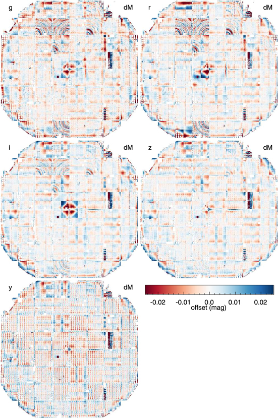
Figure 2. High-resolution flat-field correction images for the five filters grizy. These images are shown in standard camera orientation with OTA00 in the lower-left corner and OTA07 in the upper-right corner. Fine "tree-ring" structures are visible in several chips, especially in the bluer bands. The effect of the central "tent" on the photometry, presumably due to the rapidly varying PSF in this region, may also be seen.
Download figure:
Standard image High-resolution imageFirst, at the center of the camera is an important structure caused by the telescope optics, which we call the "tent." In this portion of the focal plane, the image quality degrades very quickly. The photometry is systematically biased because the PSF model cannot follow the real changes in the PSF shape on these small scales. As is evident in the image, the effect is such that the flux measured using a PSF model is systematically low, as expected if the PSF model is too small.
The square outline surrounding the "tent" is due to the 2 × 2 sampling per chip used for the ubercal flat-field corrections. The imprint of the ubercal flat field is visible throughout this high-resolution flat field: in regions where the underlying flat-field structure follows a smooth gradient across a chip, the ubercal flat field partly corrects the structure, leaving behind a sawtooth residual. The high-resolution flat field corrects the residual structures well.
Especially notable in the bluer filters is a pattern of quarter circles centered on the corners of the chips. These patterns are similar to the "tree rings" reported by the Dark Energy Survey team (Plazas et al. 2014) and identified as a result of the lateral migration of electrons in the detectors owing to electric fields due to dopant variations. Unlike the tree-ring features discussed by these other authors, the strong features observed in the GPC1 photometry are not caused by lateral electric fields but rather by variations in the vertical electron diffusion rate due to electric field variations perpendicular to the plane of the detector. This effect is discussed in detail by Magnier et al. (2018). The photometric features are due to low-level changes in the PSF size, which we attribute to the variable charge diffusion.
Other features include some poorly responding cells (e.g., in OTA14) and effects at the edges of chips, possibly where the PSF model fails to follow the changes in the PSF.
5.3.2. Stack and Warp Photometric Calibration
For stacks and warps, the image calibrations were determined after the relative photometry was performed on the individual chips. Each stack and each warp was tied via relative photometry to the average magnitudes from the chip photometry, as described below. In this case, no flat-field corrections were applied. For the stacks, such a correction would not be possible after the stack has been generated because multiple chip coordinates contribute to each stack pixel coordinate. For the warps, it is in principle possible to map back to the corresponding chip, but the information was not available in the DVO database, and thus it was not possible at this time to determine the flat-field correction appropriate for a given warp. This latter effect is one of several that degrade the warp photometry compared to the chip photometry at the bright end.
For the stack calibration, we calculate two separate zero-points: one for photometry tied to the PSF model and a second for the aperture-like measurements (total aperture magnitudes, Kron magnitude, circular fixed-radius aperture magnitudes). This split is needed because of the limited quality of the stack PSF photometry due to the highly variable PSF in the stacks. Aperture magnitudes, however, are not significantly affected by the PSF variations. We therefore tie the PSF magnitudes to the average of the chip photometry PSF magnitudes, but the aperture-like magnitudes are tied by equating the stack Kron magnitudes to the average chip Kron magnitudes.
5.4. Object Photometry
Once the image photometric calibrations (zero-points and flat-field corrections) have been determined and applied to the measurements from each image, we can calculate the best average photometry for each object. We calculate average magnitudes for the chip photometry; for the forced-warp photometry, we calculate the average of the fluxes and report both average fluxes and the equivalent average magnitudes. Because the chip photometry requires a signal-to-noise ratio of 5 for a detection, the bias introduced by averaging magnitudes is small. As the forced-warp photometry measurements have low signal-to-noise ratio, with potentially negative flux values, it is necessary to average the fluxes.
The first challenge is to select which measurements to use in the calculation of the average photometry. For the 3π Survey data, a single object may have anywhere from zero to roughly 20 measurements in a given filter. Not all measurements are of equal value, but we need a process that assigns an average photometry value in all cases (and a way for the user to recognize average values that should be treated with care). As discussed in more detail below, we have defined a triage process to select the "best" set of measurements available in each filter for each object. Once the set of measurements to be used in the analysis is determined, we use the iteratively reweighted least-squares (IRLS) technique (see, e.g., Green 1984) to determine the average photometry given the possible presence of non-Gaussian outliers even within the best subset of measurements.
5.4.1. Selection of Measurements
To choose the measurements that will be used in the analysis, we give each measurement a rank value based on a variety of tests of the quality of the measurement, with lower values being better quality. In the description below, the ranking values are defined as follows:
- 1.rank 0: perfect measurement (no quality concerns)
- 2.rank 1: PSF "perfect pixel" quality factor (PSF_QF_PERFECT) < 0.85. PSF_QF_PERFECT measures the PSF-weighted fraction of pixels that are not masked (see Paper IV).
- 3.rank 2: photometry analysis flag field (photFlags) has one of the "poor-quality" bits raised. These bits are listed below; OR-ed together, they have the hexadecimal value 0xe0440130.
- (a)PM_SOURCE_MODE_POOR = 0x00000010: fit succeeded, but with low signal-to-noise ratio or high chi-square
- (b)PM_SOURCE_MODE_PAIR = 0x00000020: source fitted with a double PSF
- (c)PM_SOURCE_MODE_BLEND = 0x00000100: source is a blend with other sources
- (d)PM_SOURCE_MODE_BELOW_MOMENTS_SN = 0x00040000: moments not measured due to low signal-to-noise ratio
- (e)PM_SOURCE_MODE_BLEND_FIT = 0x00400000: source was fitted as a blended object
- (f)PM_SOURCE_MODE_ON_SPIKE = 0x20000000: peak lands on diffraction spike
- (g)PM_SOURCE_MODE_ON_GHOST = 0x40000000: peak lands on ghost or glint
- (h)PM_SOURCE_MODE_OFF_CHIP = 0x80000000: peak lands off edge of chip
- 4.rank 3: poor measurement as defined by relphot. This may be due to a fixed allowed region on the detector or due to an outlier clipped analysis. In the 3π PV3 calibration, these tests were not applied.
- 5.rank 4 : PSF quality factor (PSF_QF) < 0.85. PSF_QF measures the PSF-weighted fraction of pixels which are not masked as "bad," but may be "suspect." Bad values are blank, highly nonlinear, or nonresponsive; suspect pixels include those pixels on ghosts, diffraction spikes, bright-star bleeds, and the mildly saturated cores of bright stars. Suspect values may have some use in measuring a flux, but with caution (see Papers II and III).
- 6.rank 5: photometric calibration of the GPC1 exposure is determined by relphot to be poor. This situation occurs if there are too few stars available for the calibration (<10 selected stars, or if the selected stars account for <5% of all stars in the exposure). An exposure may also be identified as poor if the zero-point is excessively deviant (>2 mag from the nominal value) or if the standard deviation of the calibration residuals is more than twice the median standard deviation for all exposures.
- 7.rank 6 : photometry analysis flag field (photFlags) has one of the "bad-quality" bits raised. These bits are listed below; OR-ed together they have the hexadecimal value 0x1003bc88.
- (a)PM_SOURCE_MODE_FAIL = 0x00000008: nonlinear fit failed (nonconverge, off-edge, run to zero)
- (b)PM_SOURCE_MODE_SATSTAR = 0x00000080: source model peak is above saturation
- (c)PM_SOURCE_MODE_BADPSF = 0x00000400: failed to get good estimate of object's PSF
- (d)PM_SOURCE_MODE_DEFECT = 0x00000800: source is thought to be a defect
- (e)PM_SOURCE_MODE_SATURATED = 0x00001000: source is thought to be saturated pixels (bleed trail)
- (f)PM_SOURCE_MODE_CR_LIMIT = 0x00002000: source has crNsigma above limit
- (g)PM_SOURCE_MODE_MOMENTS_FAILURE = 0x00008000: could not measure the moments
- (h)PM_SOURCE_MODE_SKY_FAILURE = 0x00010000: could not measure the local sky
- (i)PM_SOURCE_MODE_SKYVAR_FAILURE = 0x00020000: could not measure the local sky variance
- (j)PM_SOURCE_MODE_SIZE_SKIPPED = 0x10000000: size could not be determined
- 8.rank 7: measurement is from an invalid time period or photometry code. This rank level is not used in the 3π PV3 calibration. Measurements were not restricted on the basis of the time of the observation, and only GPC1 measurements were explicitly included.
- 9.rank 8: instrumental magnitude out of range. This rank level was not used in the 3π PV3 calibration.
Rank values are assigned exclusively starting from the highest values: if a measurements satisfies the rule for, e.g., rank 6, it will not be tested for ranks 5 and lower. After all measurements have been assigned a ranking value, the set of all measurements with the common lowest value are selected to be used for the average photometry analysis. If measurements from ranks 0 through 4 were used for the average photometry for a given filter, a per-filter mask bit value is raised identifying which rank was used. These bits are called ID_SECF_RANK_0 through ID_SECF_RANK_4 (see Table 2). This assessment of the valid measurements is performed independently for PSF, Kron, and seeing-matched total aperture magnitudes. All measurements that are retained to determine the average value are marked with bit flags: ID_MEAS_PHOTOM_PSF, ID_MEAS_PHOTOM_KRON, or ID_MEAS_PHOTOM_APER depending on which average magnitude is being calculated.
5.4.2. Iteratively Reweighted Least-squares Fitting
With an automatic process applied to hundreds of millions of objects, it is important for the analysis to provide a measurement of the photometry of each object that is robust against failures or other outliers. We would like to calculate an average magnitude for each filter under the assumption that the flux of the star is constant and all measurements are drawn from that population. However, even after rejecting bad measurements based on the quality information above, individual measurements may still be deviant. The Pan-STARRS1 detections have a relatively high rate of non-Gaussian outliers, partly because of the wide range of instrumental features affecting the data (see Paper III). We have used IRLS fitting to reduce the sensitivity of the fits to outlier measurements.
We have also used bootstrap resampling to determine confidence limits on our fits given the observed collection of photometry measurements. In this case, the analysis is fitting the trivial model that the photometry measurements are derived from a population with an underlying constant value. The discussion below applies to both the average of the chip photometry magnitudes and the forced-warp photometry fluxes. This technique is used to calculate the average magnitudes for all three types of photometry stored in the DVO database: PSF, Kron, and seeing-matched total aperture photometry.
Iteratively reweighted least-squares fitting describes a class of parameter estimation techniques in which weights are modified compared to those derived from the standard error in order to improve the speed of convergence or the robustness to deviant measurements. Broad reviews of these techniques can be found in Green (1984) and Street et al. (1988). In our implementation, the IRLS analysis starts with an ordinary least-squares fit, using the weights for each measurement as determined from Poisson statistics. Because our model is a constant flux, this step is equivalent to calculating a simple weighted average.
Next, the deviations from the average value for each photometry measurement are calculated. The deviation, normalized by the Poisson error, is used to modify the standard weight. We use a Cauchy function to define a new weight:

using

where Fo is the average magnitude (or flux for forced-warp photometry), Fi is the measured magnitude (or flux), σ is the standard Poisson-based error on the photometry measurement, and ω is the ordinary Poisson weight (σ−2). This modified weight has the behavior that if the observed photometry differs from the model by a substantial amount, the weight is greatly reduced, while the weight approaches the standard weight if the model and observed positions agree well. Thus, this procedure is equivalent to sigma clipping but allows the impact of the outliers to be reduced in a continuous way, rather than rigidly accepting or rejecting them.
The weighted-average photometry is recalculated with these modified weights. New values for ω are calculated, and the weighted average is calculated again. In each iteration, the weighted-average photometry values are compared to the values from the previous iteration. If they have not changed significantly (<10−6) or if the fractional change is less than some tolerance (10−4), then iterations are halted and the last weighted-average values are used. If convergence is not reached in 10 iterations, the process is halted in any case and a flag raised for the object to note that IRLS did not converge.
To calculate a fit χ2 value and to determine an appropriate set of errors for the model parameters, it is necessary to transform the modified weights into explicit cuts. We have used the rubric that if the modified weight is less than 30% of the median weight (ω' < 0.3〈ω〉) then the point is treated as clipped. The χ2 is determined from the remaining unclipped points using the standard Poisson errors. Data points that are so excluded are marked with bit flags: ID_MEAS_MASKED_PSF, ID_MEAS_MASKED_KRON, or ID_MEAS_MASKED_APER depending on which average magnitude is being calculated.
Bootstrap-resampling analysis is used to assess the errors on the fit parameters: a number of measurements equal to the number of remaining unclipped data points are randomly selected from the set of unclipped data points, with replacement after each selection. These data points are then used to calculate the weighted-average photometry. The average values are recorded and the process rerun 100 times. The error on the photometry value is determined as half of the 68% confidence range for the distribution of average values. However, if the number of measurements is small, the bootstrap-resampled measurement of the error may be artificially small. We record the maximum of the bootstrap-sampling error and the formal error from the weighted-average calculation. The minimum and maximum of the unclipped values are also recorded for the chip photometry.
One detail related to the above analysis concerns the measurements from images that were included in the ubercal analysis. These images were determined to have been taken in good-quality (photometric) weather and have had their zero-points determined with a robust analysis. We therefore overweight these data points to ensure the average photometry is dominated by the ubercal values. In the IRLS analysis above, the ubercal points are given 10 times the weight of the non-ubercal points. This overweighting is applied independently of the calculation of the reweighting based on the deviation from the model. Thus, the increased weight is not applied by reducing the error bars by a factor of 10 because that would increase the chance that the ubercal measurements would be given reduced weight. If the average photometry of an object in a filter includes ubercal measurements, the per-filter bit flag ID_SECF_USE_UBERCAL is set.
5.4.3. Stack Photometry
For the stack photometry, the assessment is different from the chip and forced-warp photometry: multiple measurements are not used to calculate an average value. For most of the sky, only a single set of stack pixels exists for each filter. Ideally, a unique astronomical object would only be detected once in a given filter, resulting in only a single measurement of that object from that filter's stack in the database. In practice, objects within a single stack image are occasionally split by the analysis code, resulting in multiple detections of the same object. This situation is discussed in more detail below.
In addition to the these relatively rare failure cases, the objects detected in the stacks may also have multiple measurements due to the overlap between neighboring stack images. The skycells (within which the stacks are generated) for a given projection cell are defined to have significant overlap between neighbors to ensure that a modestly extended object can be measured completely on the pixels in a single skycell image. For the RINGS.V3 skycell tessellation used for the 3π PV3 analysis, this overlap was set to be 60'', i.e., 240 extra pixels on each edge. Within RINGS.V3, projection cells themselves are defined to have an overlap with neighboring projection cells to avoid gaps due to the process of tiling the spherical sky with a series of flat projections. Due to the curved surface of the sky, the amount of overlap between projection cells increases away from the celestial equator. Figure 3 illustrates both skycell and projection cell overlaps.
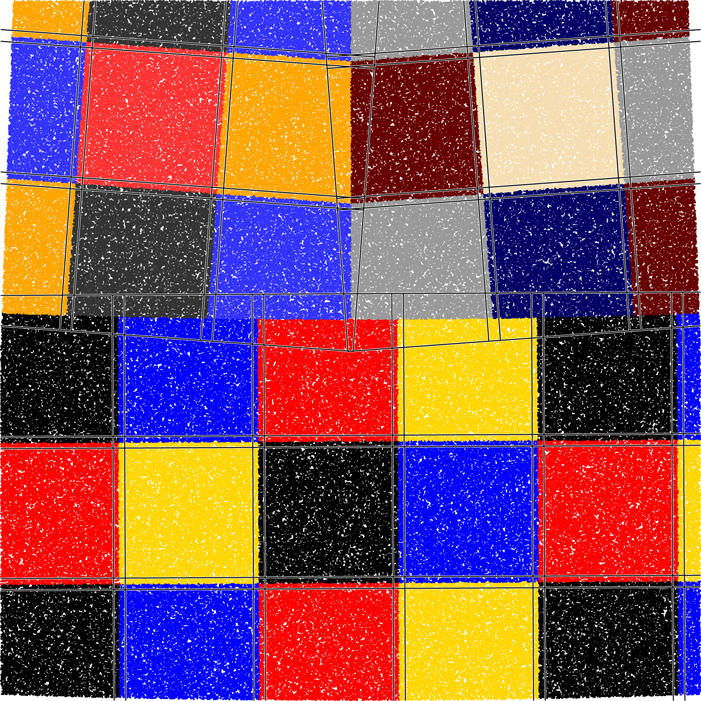
Figure 3. Illustration of overlapping skycells and the identification of the "primary" detections.
Download figure:
Standard image High-resolution imageOverlapping stack regions are not statistically independent. In the typical circumstance, the same raw chip images are used to generate the input warp images for the skycell on either side of the overlap. Except for rare edge cases (e.g., an input warp that was rejected from the stack for one side but not the other), exactly the same input raw chip pixels contribute to all sets of stack pixels which overlap. It would therefore be statistically inappropriate to average the multiple stack measurements from different overlapping skycells. Instead, we identify a unique set of stack measurements for the end user.
We identify two different ways in which an appropriate set of unique stack measurements can be selected. In the first case, if multiple overlapping skycells contribute measurements to an object, we choose the representative measurement based on their location in the skycell. This selection is purely a function of the geometry of the skycells and the coordinate of the object. We first identify the primary projection cells, those for which the overlapping regions are closest to the projection cell center. For regions in the primary projection cell, we then identify the primary skycells, those for which the overlapping regions are closest to the center of the skycell. For a given object, the identification of the primary projection cell and skycell is calculated based on that the coordinates of the object. We then find the measurements for the object that came from the primary projection cell and skycell and identify this set of measurements ( ,
,  ,
,  ,
,  ,
,  ) as the "primary" set. Note that we use the average position of the object to define the "primary" measurements, forcing measurements from all filters for the same skycell to be "primary" measurements, even if small deviations in the stack positions would result in one of the filter detections falling on the other side of the skycell "primary" boundary. Thus, for a given object in the database, we expect all five filters to provide a "primary" measurement from the same skycell for each object. Also note that a faint object, near the detection limit of the stack, may be detected on a secondary skycell but not (due to statistical fluctuations) be detected on the corresponding primary skycell. Thus, it is expected that some objects may be lacking any primary detections.
As the "primary" identification is purely based on the skycell geometry and the coordinate of the object, there is no guarantee that any primary measurement is in fact the best or even a good measurement of the object. While the different overlapping pixels should be essentially identical, it is possible (due to some of the edge cases mentioned above) that one of the two sets of pixels is more heavily masked than the other (e.g., more rejected inputs to the stack). Thus, it is possible that one of the measurements is valid while the other is not. To address this possibility, we also identify a set of "best" measurements for each object.
For the stack measurements of an object in a specific filter, if there are "primary" measurements with finite signal-to-noise ratio and PSF "perfect pixel" quality factor (PSF_QF_PERFECT) > 0.95, the measurement with the highest signal-to-noise ratio is marked as "best." If no primary measurement has PSF_QF_PERFECT > 0.95 but a secondary measurement does, then the secondary measurement with the highest signal-to-noise ratio is chosen as "best." If neither of the first two cases hold, but there exist primary measurements with lower PSF_QF_PERFECT values, the measurement with the highest PSF_QF_PERFECT value is chosen as "best." Finally, if no "best" value has yet been identified, the secondary measurement with the highest value of PSF_QF_PERFECT is chosen as "best." Note that the above rules allow for multiple measurements of the same object from the same skycell pixels. This may occur if the object was split due to, e.g., saturation or complex morphology. This type of split should not be common (and in fact reflects a failure of the algorithm), but we have defined the rules to allow us to choose an acceptable measurement even in these cases. Also note that the "best" measurement is not guaranteed to be a good measurement.
Stack measurements that are in the "primary" skycell have the bit flag ID_MEAS_STACK_PRIMARY. The measurement that was identified as the "best" measurement gets the bit flag ID_MEAS_STACK_PHOT_SRC. If a "primary" measurement exists for a given filter, then the per-filter bit flag ID_SECF_STACK_PRIMARY is set for that filter. If multiple primary stack measurements exist for a given filter, then the per-filter bit flag ID_SECF_STACK_PRIMARY_MULTIPLE is also set for that filter. If the "best" measurement for a filter is a significant detection (not forced from another band), then the per-filter bit flag ID_SECF_STACK_BESTDET is set. If any of the "primary" measurements for a filter is a significant detection (not forced from another band), then the per-filter bit flag ID_SECF_STACK_PRIMDET is set. If any stack measurements exist for a given filter, then the per-filter bit flag ID_SECF_HAS_PS1_STACK is set.
The "best" stack measurements are examined across the filters. If for all five filters the "best" stack measurement is a "primary" measurement, then the object bit flag ID_OBJ_BEST_STACK is set. If the "best" stack measurement in a filter has signal-to-noise ratio less than 5, has any of the "bad-quality" bits raised (see Section 5.4.1, rank 6), or has a PSF_QF value less than 0.85 (or NAN), it is considered to be "bad." If it has any of the "poor-quality" bits raised (see Section 5.4.1, rank 2), or has a PSF_QF_PERFECT value less than 0.85, it is considered to be "suspect." Otherwise, the measurement is considered to be "good." For an object detected in the stacks, if at least two of the filters have "good" stack measurements, then the object is considered to be "good," i.e., likely to be a valid astronomical object, and the object bit flag ID_OBJ_GOOD_STACK is set. If no more than one filter measurement is good, and there are at least two good or suspect measurements, then the object is considered to be "suspect" and the object bit flag ID_OBJ_SUSPECT_STACK is set. If at most a single measurement is either good or suspect, then the object is considered to be "bad" and the object bit flag ID_OBJ_BAD_STACK is set. Note, however, that a high-redshift quasar that is well detected in the  band but undetected in the other bands would be labeled "bad"; caution is required as always.
The public science database (PSPS) available through the MAST interface includes two fields in the StackObjectThin table, primaryDetection and bestDetection. These fields have an error in their definition and should not be used for either DR1 or DR2. An update to the database will define fields for each object which encapsulate the information about the "primary" and "best" detections. Users should consult the help pages at MAST for further information.
5.4.4. Warp Photometry
The calculation of the average forced-warp photometry is performed very similarly to the average of the chip photometry, with two important exceptions. First, as discussed above, the forced-warp fluxes are averaged, rather than the magnitudes. Second, only the warp measurements from the skycell that provided the "best" stack measurements are used to calculate the average. Just as the overlapping stack pixels are not statistically independent, overlapping warp pixels from the same exposure are also not statistically independent. It is critical to use only a single measurement from each input exposure. We choose to use those from the "best" stack skycell rather than the "primary" stack skycell to ensure the forced-warp photometry represents the highest quality set of measurements. Once the measurements from the chosen skycell have been selected, the same quality cuts are applied to the measurements as are applied to the chip measurements, as discussed above. Forced-warp measurements actually used to calculate the average for a filter are marked with the bit flag ID_MEAS_WARP_USED.
5.4.5. Object Photometry Flags
Certain object-level bit flags are set based on the chip-stage measurements. If any object has at least one PS1 measurement from rank 0–2 (Section 5.4.1), then the object is marked with the bit flag ID_OBJ_GOOD. Each measurement is also checked for consistency with a PSF or an extended source morphology: if the difference between the PSF magnitude and the seeing-matched full aperture magnitude is less than a specific cutoff (2.5σ added in quadrature to a floor of 0.1 mag), then the measurement is considered "PSF like." Otherwise, the measurement is counted as extended. If more of the PS1 measurements are extended than PSF like, the object bit flag ID_OBJ_EXT is raised. If more than half of the PS1 chip-stage measurements within a single filter are extended, then the per-filter bit flags ID_SEC_OBJ_EXT and ID_SEC_OBJ_EXT_PSPS are set. The latter bit is a duplicate bit defined because the high bit in a 32 bit integer is difficult to handle within the context of an SQL server. Any object that has any chip-stage measurements for one of the five filters has the per-filter bit flag ID_SECF_HAS_PS1 set. Because stack images are more sensitive than the individual exposures, faint sources that are detected in only the stacks will have the bit flag ID_SECF_HAS_PS1_STACK set but not ID_SECF_HAS_PS1 as the latter only refers to individual chip detections.
In addition, if the object has measurements from the 2MASS point source catalog, the quality of these measurements is checked. If the 2MASS quality flag ph_qual has a value of A,B, or C, then the object is considered to be a good 2MASS object and the bit flag ID_OBJ_GOOD_ALT is set. If the 2MASS extended source flag, gal_contam, has a value of 1 or 2, then the object bit flag ID_OBJ_EXT_ALT is set.
We also set certain object-level bit flags based on additional analysis of the Pan-STARRS data. Hernitschek et al. (2016) used measurements from the 3π Survey to identify potentially interesting variable sources. They examined the characteristics of the varying fluxes in the five bands to distinguish two classes of variable sources: RR Lyrae stars and QSOs. They present two classifier statistics, PQSO and PRRLyrae, which can be used to select candidates with varying levels of quality and completeness. Using this catalog, we have marked objects with a set of bits to specify the possible variability information as identified by Hernitschek et al. (2016):
- 1.ID_OBJ_HERN_QSO_P60: identified as a likely QSO, PQSO ≥ 0.60
- 2.ID_OBJ_HERN_QSO_P05: identified as a possible QSO, PQSO ≥ 0.05
- 3.ID_OBJ_HERN_RRL_P60: identified as a likely RR Lyra, PRRLyra ≥ 0.60
- 4.ID_OBJ_HERN_RRL_P05: identified as a possible RR Lyra, PRRLyra ≥ 0.05
- 5.ID_OBJ_HERN_VARIABLE: identified as a variable by Hernitschek et al. (2016)
In addition, the Pan-STARRS MOPS team has identified solar system objects within the 3π data set. We have used a list of 14.7M such detections recorded by MOPS from the 3π Survey. Any object that contains one of these detections has the object bit flag ID_OBJ_HAS_SOLSYS_DET set. If 50% or more of the detections for an object are solar system objects, then the bit flag ID_OBJ_MOST_SOLSYS_DET is set.
5.5. Photometry Calibration Quality
Figure 4 shows the standard deviations of the mean residual photometry for bright stars as a function of position across the sky. For each pixel in these images, we selected all objects with (14.5, 14.5, 14.5, 14.0, 13.0) < (g, r, i, z, y) < (17, 17, 17, 16.5, 15.5) magnitudes, with at least three measurements in the i band (to reject artifacts detected in a pair of exposures from the same night), with PSF_QF > 0.85 (to reject excessively masked objects), and with magPSF − magKron < 0.1 (to reject galaxies). We then generated histograms of the difference between the average magnitude and the apparent magnitude in an individual image for each filter for all stars in a given pixel in the images. From these residual histograms, we can then determine the median and the 68th percentile range to calculate a robust standard deviation. This represents the bright-end systematic error floor for a measurement from a single exposure. The standard deviations are then plotted in Figure 4.
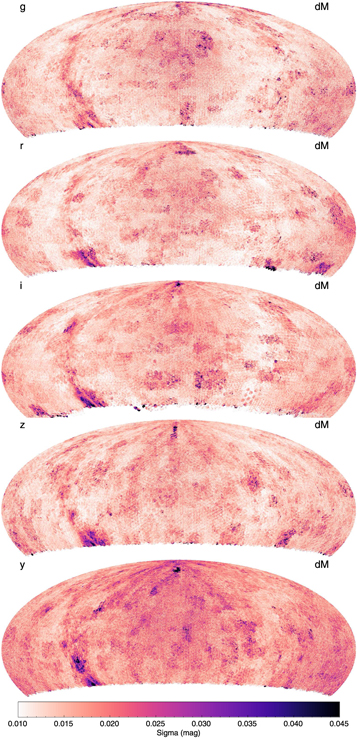
Figure 4. Consistency of photometry measurements across the sky. Each panel shows a map of the standard deviation of photometry residuals for stars in each pixel. The median value of the measure standard deviations across the sky is (σg , σr , σi , σz , σy ) = (14, 14, 15, 15, 18) mmag. These values reflect the typical single-measurement errors for bright stars.
Download figure:
Standard image High-resolution imageThe five panels in Figure 4 show several features. The Galactic bulge is clearly seen in all five filters, with the impact strongest in the reddest bands. We attribute this to the effects of crowding and contamination of the photometry by neighbors. Large-scale, roughly square features ≈10° on a side in these images can be attributed to the vagaries of weather: these patches correspond to the observing chunks. These images include both photometric and nonphotometric exposures. It seems plausible that the nonphotometric images from relatively poor-quality nights elevate the typical errors. On small scales, there are circular patterns ≈3° in diameter corresponding to individual exposures; these represent residual flat-field structures not corrected by our stellar flat-fielding. The median of the standard deviations in the five filters are (σg , σr , σi , σz , σy ) = (14, 14, 15, 15, 18) mmag.
As discussed above (Section 5.3.2), the DR2 stack calibration used separate zero-points for PSF-like and aperture-like photometry. For DR1, this split zero-point calibration was not used. Instead all stack photometry was tied to the average chip photometry via the PSF magnitudes. The result of using a single zero-point is that the stack PSF magnitudes are consistent across the sky with the chip PSF magnitudes, but the aperture-like magnitudes show significant spatial variations. A second issue identified in DR1 and corrected in DR2 is due to the application of the high-resolution photometric flat-field correction. For the initial processing of the PV3 calibration, this flat-field correction was applied with the wrong sign. For DR1, the error was corrected for the chip-stage photometry. However, the stack and warp photometry had been tied to the chip-stage photometry before this correction, and they were not recalibrated before the DR1 release. After this error was noticed, the stack and warp photometry were recalibrated for DR2. Figure 5 illustrates the impact of using a single PSF zero-point for the stack photometry and the impact of the flat-field error. This zero-point split is not needed for the forced-warp photometry because the individual warps have well-defined PSFs.
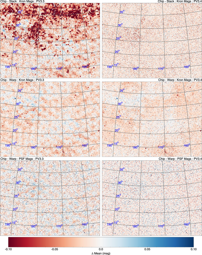
Figure 5. Sample comparison of PV3.3 and PV3.4 photometry illustrating the impact of the issues identified in the PV3.3 stack and warp photometry. All figures use  -band photometry, restricted to objects brighter than 17 mag with at least 10 chip measurements. The left panels use data from PV3.3 while the right use PV3.4. The top row shows the mean difference between the average photometry from individual exposures ("chip") and the stack photometry using Kron magnitudes. The middle row shows the mean difference between the average photometry from individual exposures ("chip") and the average forced-warp photometry, again using Kron magnitudes. The bottom row shows the mean difference between the average photometry from individual exposures ("chip") and the average forced-warp photometry, using PSF magnitudes. See Section 7 for a description of the calibration change in PV3.4.
Download figure:
Standard image High-resolution image6. Astrometry Calibration
Once the full PV3 data set is loaded into the master PV3 DVO database, along with supporting databases, and the photometric calibrations performed, relative astrometry could be performed on the database to improve the overall astrometric calibration.
In many respects, the relative astrometric analysis is similar to the relative photometric analysis: the repeated measurements of the same object in different images are used to determine a high-quality average position for the object. The new average positions are then used to determine improved astrometric calibrations for each of the images. These improved calibrations are used to set the observed coordinates of the measurements from those images, which are in turn used to improve the average positions of the objects. The whole process is repeated for several iterations. Like the photometric analysis, the astrometric analysis is performed in a parallel fashion with the same concept that specific machines are responsible for exposures and objects that land within their regions of responsibility, defined on the basis of lines of constant R.A. and decl. Between iteration steps, the astrometric calibrations are shared between the parallel machines as are the improved positions for objects controlled by one machine but detected in images controlled by another machine. Like the photometric analysis, the entire sky is processed in one pass. However, there are some important differences in the details.
6.1. Systematic Effects
First, the astrometric calibration has a larger number of systematic effects which must be corrected. These consist of (1) the Koppenhöfer effect, (2) differential chromatic refraction (DCR), and (3) static deviations in the camera. We discuss each of these in turn below.
6.1.1. Koppenhöfer Effect
The KE was first identified in 2011 February by Johannes Koppenhöfer (MPE) as part of the effort to search for planet transits in the Stellar Transit Survey data. He noticed that the astrometry of bright stars and faint stars disagreed on overlapping chips at the boundary between the STS fields. After some exploration, it was determined that the X coordinate of the brightest stars was offset from the expected location based on the faint stars for a subset of the GPC1 chips. The essence of the effect was that a large charge packet could be drawn prematurely over an intervening negative serial phase into the summing well, and this leakage was proportionately worse for brighter stars. The brighter the star, the more the charge packet was pushed ahead on the serial register. The amplitude of the effect was at most 025, corresponding to a shift of about one pixel. This effect was only observed in two-phase OTA devices, with 22/30 of these suffering from this effect. By adjusting the summing well high voltage down from a default +7V to +5.5V on the two-phase devices, the effect was prevented in exposures after 2011 May 3. However, this left 101,550 exposures (27%) already contaminated by the effect.
We measured the Koppenhöfer effect by accumulating the residual astrometry statistics for stars in the database. For each chip, we measured the mean X and Y displacements of the astrometric residuals as a function of the instrumental magnitude of the star divided by the FWHM2. We measured the trend for all chips in a number of different time ranges and found the effect to be quite stable, in the period where it was present. The effect only appeared in the serial direction. Figure 6 shows the Koppenhöfer effect trend for a typical affected chip both before and after the correction. Figure 7 shows the maximum impact of the Koppenhöfer effect as a function of chip position in the focal plane. For the PV3 data set, we remeasured the Koppenhöfer effect trends using stars in the Galactic pole regions after an initial relative astrometry calibration pass: the Galactic pole is necessary because the real-time astrometric calibration relies largely on the fainter stars which are not affected by the Koppenhöfer effect. The trend is then stored in a form that can be applied to the database measurements.
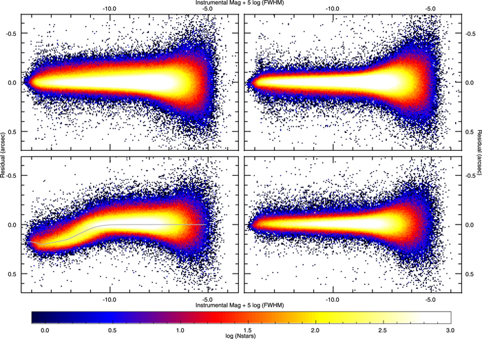
Figure 6. Illustration of the Koppenhöfer effect on OTA04. Bottom left: X direction before correction. The solid line shows the measured mean residual for stars detected on this chip as a function of the instrumental magnitude/FWHM2. Bottom right: Y direction before correction. Top left: X direction after correction. Top right: Y direction after correction.
Download figure:
Standard image High-resolution image
Figure 7. Map of the amplitude of the Koppenhöfer effect on chips across the focal plane. In the affected chips, bright stars are up to 02 deviant from their expected positions. Bottom left: X direction before correction. Bottom right: Y direction before correction. Top left: X direction after correction. Top right: Y direction after correction.
Download figure:
Standard image High-resolution image6.1.2. Differential Chromatic Refraction
DCR affects astrometry because the reference stars used to the calibrate the images are not the same color as the rest of the stars in the image. For a given star of a color different from the reference stars, as exposures are taken at higher airmass, the apparent position of the star will be shifted along the parallactic angle. While it is possible to build a model for the DCR impact based on the filter response functions and atmospheric refraction, we have instead elected to use an empirical correction for the DCR present in the PV3 database. We have measured the DCR trend using the astrometric residuals of millions of stars after performing an initial relative astrometry calibration. We define a blue DCR color (g − i) to be used when correcting the filters  ,
,  , and
, and  , and a red DCR color (z − y) to be used when correcting the filters
  and
and  . In the process of performing the relative astrometry calibration, we record the median red and blue colors of the reference stars used to measure the astrometry calibration for each image. As we determine the astrometry parameters for each object in the database, we record the median red and blue reference star colors for all images used to determine the astrometry for a given object. For each star in the database, we know both the color of the star and the typical color of the reference stars used to calibrate the astrometry for that star.
We measure the mean deviation of the residuals in the parallactic angle direction and the direction perpendicular to the parallactic angle. For each filter, we determine the DCR trend as a function of the difference between the star color and the reference star color, using the red or blue color appropriate to the particular filter, times the tangent of the zenith distance:


where (g − i)ref and (z − y)ref are the median colors of the stars used to calibrate a specific blue- or red-filter image, respectively, while ζ is the zenith distance. Figure 8 shows the DCR trend for the  filter as an example, as well as the measured displacement in the direction perpendicular to the parallactic angle. We represent the trend with a spline fitted to this data set.
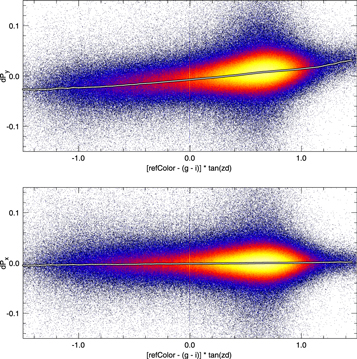
Figure 8. Example of the DCR trend in the g band, in which it is strongest. Top: DCR trend in the parallactic direction. Bottom: DCR trend perpendicular to the parallactic angle.
Download figure:
Standard image High-resolution imageThe amplitude of the DCR trend, α, in the five filters is (g, r, i, z, y) = (0010, 0001, −0003, −0017, −0021) airmass−1 magnitude−1. We saturate the DCR correction if the term ![$\left[{(g-i)}_{\mathrm{ref}}-(g-i)\right]\tan \zeta $](https://content.cld.iop.org/journals/0067-0049/251/1/6/revision3/apjsabb82aieqn59.gif) or
or ![$\left[{(z-y)}_{\mathrm{ref}}-(z-y)\right]\tan \zeta $](https://content.cld.iop.org/journals/0067-0049/251/1/6/revision3/apjsabb82aieqn60.gif) for a given measurement is outside of the range where the DCR correction is measured. The maximum DCR correction applied to the five filters is (g, r, i, z, y) = (0019, 0002, 0003, 0006, 0008).
for a given measurement is outside of the range where the DCR correction is measured. The maximum DCR correction applied to the five filters is (g, r, i, z, y) = (0019, 0002, 0003, 0006, 0008).
6.1.3. Astrometric Flat Field
After correction for both Koppenhöfer effect and DCR, we observe persistent residual astrometric deviations that depend on the position in the camera. We construct an astrometric "flat-field" response by determining the mean residual displacement in the X and Y (chip) directions as a function of position in the focal plane. We have measured the astrometric flat using a sampling resolution of 80 × 80 pixels. Figures 9 and 10 show the astrometric flat-field images for the five filters  ,
,  ,
,  ,
,  , and
, and  in each of the two coordinate directions. These plots show several types of features.
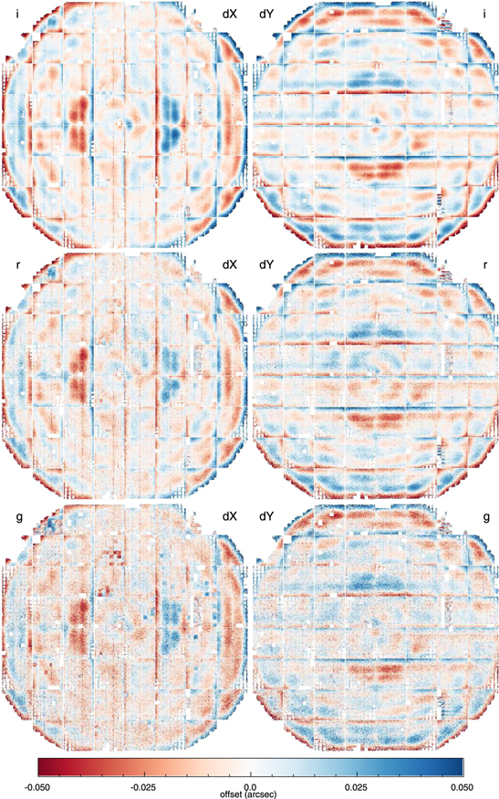
Figure 9. High-resolution astrometric flat-field correction images for gri.
Download figure:
Standard image High-resolution image
Figure 10. High-resolution astrometric flat-field correction images for zy.
Download figure:
Standard image High-resolution imageThe dominant pattern in the astrometric residual is roughly a series of concentric rings. The pattern is similar to the pattern of the focal surface residuals measured by Onaka et al. (2008), which also has a concentric series of rings with similar spacing. The "tent" in the center of the focal surface is reflected in these astrometry residual plots. Our interpretation of the structure is that the deviations of the focal plane from the ideal focal surface introduce small-scale PSF changes, presumably coupled to the optical aberrations, which result in small changes in the centroid of the object relative to the PSF model at that location. Because the PSF model shape parameters are only able to vary at the level of a 6 × 6 grid per chips, the finer structures are not included in the PSF model.
The PV2 analysis shows this circular pattern more clearly than the PV3 analysis, with a pattern much more closely following the focal surface deviations. In the PV2 analysis, the PSF model used at most a 3 × 3 grid per chip to follow the shape variations, so any changes caused by the optical aberrations would be less well modeled in the PV2 analysis than the PV3 analysis. For PV3, some of these patterns are suppressed by the higher-resolution PSF model.
A second pattern that is weakly seen in several chips consists of consistent displacements in the X (serial) direction for certain cells. This effect can be seen most clearly in chips OTA45 and OTA46. In the PV2 analysis, this pattern is also more clearly seen. In this case, the fact that the astrometric model used polynomials with a maximum of third order per chip means the deviation of individual cells cannot be followed by the astrometric model.
A third effect is seen at the edge of the chips, where there appears to be a tendency for the residual to follow the chip edge. The origin of this is unclear but likely caused by the astrometry model failing to follow the underlying variations because of the need to extrapolate to the edge pixels.
Finally, we also mention an interesting effect not visible at the resolution of these astrometric flat-field images. Fine structures are observed at the ≈10 pixel scale similar to the "tree rings" reported by the Dark Energy Survey team (Plazas et al. 2014) and identified as a result of the lateral diffusion of electrons in the detectors due to electric fields due to dopant variations. Unlike the photometric tree-ring features discussed above (Section 5.3.1), these astrometric tree rings appear to correspond to the features identified by the DES team. Lateral electric fields in the detector silicon, caused by variations in the dopant density, cause the photoelectrons to migrate laterally in the detector silicon before landing in the pixel wells. This migration affects the apparent position of the stars, thus affecting the observed astrometry. A simple lateral translation of the effective pixel locations would not be detected as it would be degenerate with the astrometric solution. However, because the lateral electric fields, and thus the electron migration, vary with position, the astrometric displacement changes on small scales relative to the average solution, resulting in residual astrometric structures. The gradient of the astrometric displacement results in an apparent expansion or compression of the pixel sizes, generating a signal that can be observed in the flat-field images. For GPC1, unlike the DES detectors, the amplitude of these flat-field variations is much smaller than the photometric variations caused by the changing PSF sizes, caused in turn by varying electron diffusion rates. These features, and the related vertical electron diffusion variations, are discussed in detail in Magnier et al. (2018).
After the initial analysis to measure the Koppenhöfer effect corrections, DCR corrections, and astrometric flat-field corrections, we applied these corrections to the entire database. Within the schema of the database, each measurement in the Measure table has the raw chip coordinates (Xccd, Yccd) as well as the offset for that object based on each of the three corrections discussed above (XoffKH, YoffKH; XoffDCR, YoffDCR; XoffCAM, YoffCAM). The offsets are calculated for each measurement based on the observed instrumental chip magnitudes and FWHM for the Koppenhöfer effect, on the average chip colors and the altitude and azimuth of each measurement for the DCR correction, and on the chip coordinates for the astrometric flat-field corrections. The corrections are combined and applied to the raw chip coordinates and saved back in the database in the fields Xfix, Yfix. At this point, we are ready to run the full astrometric calibration.
6.2. Absolute Calibration
The analysis of the PV2 astrometry used the 2MASS positions as an inertial constraint: the 2MASS coordinates were included in the calculation of the mean positions for the objects in the database, with weight corresponding to the reported astrometric errors. In this analysis, the object positions used to determine the calibrations of the image parameters ignored proper motion and parallax. After the image calibrations were determined, individual objects were then fitted for proper motion and possibly parallax, as discussed in detail below.
Using the PV2 analysis of the astrometry calibration, we discovered large-scale systematic trends in the reported proper motions of background quasars. This motion had an amplitude of 10–15 mas per year and clear trends with Galactic longitude. We also observed systematic errors of the mean positions with respect to the ICRF milliarcsecond radio quasar positions, with an amplitude of ≈60 mas, again with trends associated with Galactic longitude. Because the 2MASS data were believed to have minimal average deviations relative to the ICRF quasars, this latter seemed to be a real effect.
We realized that both the proper motion and the mean position biases could be caused by a single common effect: the proper motion of the stars used as reference stars between the 2MASS epoch (≈2000) and PS1 epoch (≈2012). Because we are fitting the image calibrations without fitting for the proper motions of the stars, we are in essence forcing those stars to have proper motions of 0.0. The background quasars would then be observed to have proper motions corresponding to the proper motions of the reference stars, but in the opposite direction. We demonstrated that the observed quasar proper motions agreed well with the distribution expected if the median distance to our reference stars was ≈500 pc.
For the PV3 analysis, we desired to address this bias by including our knowledge about the distances to the reference stars and the expected typical proper motions for stars at those distances. With some constraint on the distance to each star, we can determine the expected proper motion based on a model of the Galactic rotation and solar motions. We can then calculate the mean positions for the objects keeping the assumed proper motion fixed. When calibrating a specific image, the reference star mean position is then translated to the expected position at the epoch of that image. The image calibration is then performed relative to these predicted positions. This process naturally accounts for the proper motion of the reference stars. In order to make the calibrations consistent with the observed coordinates of an external inertial reference, we perform the iterative fits using the technique as described, but assign very high weights in the initial iterations to the inertial reference, and reduce the weights as the astrometric calibration iterations proceed.
In order to perform this analysis, we need estimated distances for every reference star used in the analysis. Green et al. (2014) performed spectral energy distribution (SED) fitting for 800M stars in the 3π region using PV2 data. The goal of this work was to determine the 3D structure of the dust in the galaxy. By fitting model SEDs to stars meeting a basic data quality cut, they determined the best spectral type, and thus Teff, absolute r-band magnitude, distance modulus, and extinction AV (the desired output and used to determine the dust extinction as a function of distance throughout the galaxy). We use the distance modulus determined in this analysis to predict the proper motions.
To convert the distances to proper motions, we use the Galactic rotation parameters (A, B) = (14.82, −12.37) km sec−1 pc−1 and solar motion parameters (Usol, Vsol, Wsol) = (9.32, 11.18, 7.61) km sec−1 as determined by Feast & Whitelock (1997) using Hipparcos data. Proper motions are determined from the following:


where d is the distance and l, b are the Galactic coordinates of the star. Note that the proper motion induced by the Galactic rotation is independent of distance while the reflex motion induced by the solar motion decreases with increasing distance. Also note that this model assumes a flat rotation curve for objects in the thin disk. Any reference stars that are part of the halo population will have proper motions that are not described by this model; the mostly random nature of the halo motions should act to increase the noise in the measurement. We do not attempt to compensate for asymmetric drift in the populations with higher radial velocity dispersion. This effect will introduce some bias in the azimuthal direction, which our simple model cannot address. For stars for which the distance modulus is not well determined, we assume the object is simply following the Galactic rotation curve and set a fixed proper motion. If we do not have a distance modulus from the Green et al. analysis, we assume a value of 500 pc. We find that applying our Galactic rotation model improves the systematic proper motion errors to some extent. The standard deviation of the quasar proper motions (averaged on 12' superpixels across the sky) is reduced from (σμ , α, σμ , δ) = (4.6, 2.4) mas yr−1 for the uncorrected analysis to (σμ , α, σμ , δ) = (2.9, 2.0) mas yr−1 after correction for the Galactic rotation model. The remaining quasar motions continue to show some systematics, which may suggest the need to include a correction for the asymmetric drift.
For the initial PV3 analysis, we again used the 2MASS coordinates as an external astrometric reference. After the Pan-STARRS DR1 object parameters were ingested into the PSPS database, the Gaia DR1 astrometry was released (Lindegren et al. 2016). This gave us the option to use the Gaia positions for the external astrometric reference. We redid the astrometric analysis and generated a Gaia-based astrometry table for Pan-STARRS DR1. For Pan-STARRS DR2, the average object coordinates are based on the analysis using the Gaia DR1 coordinates. The Gaia DR1 coordinates used a fixed 2015 epoch. Coordinates were propagated from that epoch to the epoch for each PS1 image as described above. In a future analysis, we will use the Gaia DR2 proper motions to tie the astrometric analysis to Gaia both in terms of the mean positions as well as the dynamical system.
6.3. Object Astrometry
After the image astrometric parameters have been determined and applied to the measurements from each image, we attempt to find the best astrometric parameters (position, parallax, and proper motions) for all objects in the database. Only good-quality measurements are kept for the astrometric analysis: PS1 chip detections with PSF_QF < 0.85 are rejected, as are any detections for which the magnitude or magnitude error was reported as NAN. Only PS1 chip-stage measurements were used for the astrometry measurement (no stack or forced-warp measurements). If available, the 2MASS and Gaia DR1 astrometry for an object was also used in the calculation of the astrometry. Measurements that were kept for the astrometric fit for an object were marked with the bit flags ID_MEAS_USED_OBJ. Some detections were identified as extreme outliers if their position deviated from the mean object coordinate by more than 2''. Such a large deviation can only occur when the in-database calibration is poor, for example, near the edges of a chip. These detections were ignored and marked with the bit flag ID_MEAS_POOR_ASTROM.
If 2MASS or Gaia DR1 astrometry measurements were available for an object, all measurements for that object are marked with the bit flag ID_MEAS_OBJECT_HAS_2MASS or ID_MEAS_OBJECT_HAS_GAIA as appropriate. The Tycho 2.0 measurements were not included in this analysis and objects with Tycho measurements are therefore not marked.
6.3.1. Iteratively Reweighted Least-squares Fitting
Just as with the photometric analysis, it is also important for the astrometric analysis to provide a measurement that is robust against failures. In addition to the detector effect artifacts that affect astrometry, the astrometric measurements may have non-Gaussian outliers due to the high degree of structure in the astrometric transformations introduced by the camera optics and the atmosphere. We have again used the IRLS technique to reduce the sensitivity of the fits to outlier measurements. We have also used bootstrap resampling to determine confidence limits on our fits given the observed collection of position measurements.
We begin the astrometric analysis for each object by projecting the sky coordinates (α, δ) to a locally linear coordinate system (η, ζ). We choose as a reference a single measurement from the full set of measurements. It is not critical which measurement we choose as long as the value is recorded during the analysis so the results can be deprojected back to the sky using the same reference coordinate. We also work in a time system that has been adjusted with reference to the average epoch from the collection of measurements. The resulting proper motions are thus determined with the minimum degeneracy with respect to the average position solution.
The IRLS analysis starts with an ordinary least-squares fit, using the weights for each measurement as determined from Poisson statistics. After the astrometric parameters have been fitted, the deviations from the fit for each position are calculated for both the local η and ζ coordinate directions. The deviation, normalized by the Poisson error, is used to modify the standard weight. We use a Cauchy function to define a new weight:

using


where ηo
is the model position in the η direction, ηi
is the measured position in the η direction, ση
is the standard error on the position in the η direction, and ωη
is the ordinary Poisson weight in the η direction ( ) and equivalently for the ζ direction. This modified weight has the behavior that if the observed position differs from the model by a substantial amount, the weight is greatly reduced, while the weight approaches the standard weight if the model and observed positions agree well. Thus, this procedure is equivalent to sigma clipping but allows the outliers to be reduced in impact in a continuous way, rather than rigidly accepting or rejecting them.
The object astrometric parameters are refitted with these modified weights. New values for ωη , ωζ are calculated, and the fit is tried again. On each iteration, the fitted parameters are compared to the values from the previous iteration. If the parameters have not changed significantly (<10−6) or if the fractional change is less than some tolerance (10−4), then iterations are halted and the last fitted parameters are used. If convergence is not reached in 10 iterations, the process is halted and the analysis is rejected.
To calculate a fit χ2 value and to determine an appropriate set of errors for the model parameters, it is necessary to transform the modified weights into explicit cuts. We have used the rubric that if the modified weight is less than 30% of the standard weight ( ) then the point is treated as clipped. If a data point would be clipped based on the modified weight in either dimension, it is clipped in both (thus a point is either used to calculate both R.A. and decl. terms, or neither). The χ2 is determined from the unclipped points in the standard way. These measurements are marked with the bit flag ID_MEAS_UNMASKED_ASTRO.
Bootstrap-resampling analysis is used to assess the errors on the fit parameters in a fashion similar to the photometry analysis: a number of measurements equal to the number of the remaining unclipped data points are randomly selected from the set of the remaining unclipped data points, with replacement after each selection. These data points are then used to fit for the astrometric parameters, using ordinary least-squares fitting. The parameters are recorded and the process rerun 300 times. For each astrometric parameter, the error is determined as half of the 68% confidence range for the distribution of fitted parameter values.
6.3.2. Object Astrometry Flags
We require a minimum of five detections and 1 yr of data for any object in order for it to be fitted for just proper motion. For a parallax and proper-motion fit, we require at least seven detections, 1 yr of data, and a parallax factor range of at least 0.25; no object is fitted to a parallax without a proper motion as well. If an object is fitted for parallax, it is also fitted with a model including only proper motion and only a mean position. The chi-square for all three fits is saved. Currently, the highest order fit allowed is saved in the database, regardless of the significance of the improvement in adding parameters. The resulting parallax and proper motion measurements are inserted back into the DVO database for use by science queries. If one of the three types of fits were attempted, the corresponding bit flags are set: ID_OBJ_FIT_PAR for the full parallax fit, ID_OBJ_FIT_PM for the proper-motion fit, ID_OBJ_FIT_AVE for the mean position. The fit that was used to provide the reported astrometric parameters is noted with one of the three object bit flags: ID_OBJ_USE_PAR, ID_OBJ_USE_PM, ID_OBJ_USE_AVE. If the IRLS analysis for all three types of fits fails to converge, the raw weighted-average position is reported and the bit flag ID_OBJ_RAW_AVE is set. If the proper-motion model was attempted and failed, the bit flag ID_OBJ_BAD_PM is set.
Objects for which there is no valid chip-stage measurement (e.g., faint sources below the single-exposure detection limit) will use the position from the stack for the mean position. In this case, the bit flag ID_OBJ_STACK_FOR_MEAN will be raised. Stack astrometry is reported to the PSPS database. The stack astrometry is calculated based on the median of stack measurements. The stack measurements are not statistically independent (see Section 5.4.3), so there, an average of the stack measurements does not improve the statistical significance of the position measurement. In addition, the stack astrometry is expected to be degraded relative to the chip-stage astrometry, in part because of the geometric rewarping required to generate the stack images and in part because of the spatially variable stack PSFs. If stack measurements exist but for some reason cannot be used for astrometry (e.g., poor quality), the values reported to the PSPS database will be derived from the average of the chip detections, and the bit flag ID_OBJ_MEAN_FOR_STACK will be set for the object.
6.4. Astrometry Calibration Quality
Figure 11 shows the standard deviations of the mean residual astrometry in (α, δ) for bright stars as a function of position across the sky based on the DR2 calibration. For each pixel in these images, we selected all objects with 15 < i < 17, with at least three measurements in the i band (to reject artifacts detected in a pair of exposures from the same night), with PSF_QF > 0.85 (to reject excessively masked objects), and with magPSF − magKron < 0.1 (to reject galaxies). We then generated histograms of the difference between the object position predicted for the epoch of each measurement (based on the proper motion and parallax fit) and the observed position of that measurement, in both the R.A. and decl. directions (in linear arcseconds), for all stars in a given pixel in the images. From these residual histograms, we can then determine the median and the 68th percentile range to calculate a robust version of the standard deviation. This represents the bright-end systematic error floor for a measurement from a single exposure. The standard deviations are then plotted in Figure 11. The median value of the standard deviations across the sky in both (σα , σδ ) is 16 mas.

Figure 11. Consistency of astrometry measurements across the sky. Each panel shows a map of the standard deviation of astrometry residuals for stars in each pixel. The median value of the standard deviations across the sky is (σα , σδ ) = (16, 16) mas. These values reflect the typical single-measurement errors for bright stars. See discussion regarding the astrometric flat, which is likely responsible for these elevated values.
Download figure:
Standard image High-resolution imageThe Galactic plane is clearly apparent in these images. Like photometry, we attribute this to the failure of the PSF fitting due to crowding. The celestial north pole regions have somewhat elevated errors in both R.A. and decl., with some specific structures. Some of these structures may be due to the larger typical seeing at these high airmass regions, but some are due to astrometric failures that stem from the reference catalog based on the PV2 analysis (see Section 8 for further details). Several features which appear to be an effect of the tie to the Gaia DR1 astrometry can be seen: the stripes near the center of the decl. image and the right side of the R.A. image. The mesh of circular outlines on the 2° scale is due to the outer edge of the focal plane where the astrometric calibration is poorly determined.
The DR1 astrometric calibration suffered from degraded astrometry due to a problem with the astrometric flat-field correction identified too late to be repaired for DR1. The astrometric flat-field images used for that release had too few stars to measure the correction with sufficient signal-to-noise ratio. As a result, those corrections had significant pixel-to-pixel noise, which can be seen in Figure 12. As a result, the astrometric flat-field correction reduces systematic structures on large spatial scales but at the expense of degrading the quality of individual measurements. Only the i-band flat had sufficient signal-to-noise ratio per pixel to avoid significantly increasing the per-measurement position errors.

Figure 12. Comparison of the high-resolution astrometric flat-field images used for PV3.2 (left) and for PV3.3 (right). These examples show the  -band astrometric flat-field corrections for the X direction as seen in the focal-plane coordinate system. Note the elevated noise in the PV3.2 image due to an insufficient numbers of stars used in the analysis.
Download figure:
Standard image High-resolution imageFor DR2, we recalculated the astrometric flat-field correction using many more stars. For the DR1 release, the number of stars per filter was ( ,
,  ,
,  ,
,  ,
,  ) = (2.6M, 3.5M, 16M, 7M, 4.5M), while for the DR2 release, the number of stars per filter was (
 ,
,  ,
,  ,
,  ,
,  ) = (18M, 31M, 83M, 62M, 43M). We also reduced the resolution of the astrometric flat field, using 80 × 80 superpixels rather than the 40 × 40 superpixels used for DR1. Because of the degraded astrometric flat-field correction, the median per-measurement error floor of DR1 is ≈22 mas, significantly worse than both DR2 and the earlier PV2 analysis. Figure 13 shows histograms of the astrometric residual scatter across the sky for DR1 and DR2, illustrating the improvement.

Figure 13. Illustration of the impact of the astrometric flat-field correction used for PV3.2 vs. PV3.3. The blue histograms show the distribution of astrometric residuals for bright stars from the PV3.2 analysis while the red histograms show the distribution for the PV3.3 analysis. The median standard deviation for PV3.2 is 22 mas in R.A. (23 mas in decl.). Using the higher signal-to-noise flat-field correction images reduces the median values to 16 mas for both R.A. and decl. directions in PV3.3.
Download figure:
Standard image High-resolution image7. Discussion
7.1. Calibration Versions
The calibration of the PV3 DVO database required several iterations. For completeness, we discuss these steps and their implications for the DR1 and DR2 releases.
PV3.0—The first calibrated PV3 database is identified as PV3.0. This calibration predates the Gaia DR1 release and uses the 2MASS catalog as a reference. After internal testing, an error in the photometry calibration was identified in this DVO version: the high-resolution photometric flat-field correction measured using the stellar photometry (see Section 5.3.1) was applied with the wrong sign to the measurements.
PV3.1—After the above error was identified, the photometric flat-field correction was applied in the correct sense to the measurements and the average photometry was recalculated. The resulting PV3.1 version of the database was used for the DR1 release (but see below regarding the mean positions).
PV3.2—The Gaia DR1 release motivated a recalibration of the astrometry using the Gaia DR1 position information, combined with photometric distance estimates and a model for the Galactic and solar motion to correct the absolute proper motion (see Section 6.2). We identify the resulting database as PV3.2. This database was used to generate the positions in the gaiaObject table, which are exposed in the DR1 release.
PV3.3—After the DR1 release, we identified a problem with the astrometric flat-field corrections (see Section 6.1.3): for all but the  filter, the analysis of the flat field used too few stars. The measurement of the systematic astrometric corrections therefore had a low signal-to-noise ratio. Instead of reducing the scatter in the astrometric measurements, the application of these flat fields increased the scatter. Recognizing this error, we remeasured the astrometric flat fields with a larger number of stars and applied the improved versions to the database. The resulting PV3.3 calibration has a noticeable improvement in the astrometric scatter for bright stars.
PV3.4—Two errors were identified in the PV3.3 calibration before the DR2 release was completed. First, we discovered that the repair applied to the photometric flat-field correction for PV3.1, which reversed the sign of the correction, was not propagated to the stack or warp photometry calibrations. Although the measurements from these stages are not corrected by those flat fields, they are affected by this calibration because they are tied to the average of the chip-stage measurements. Second, we determined that the aperture-like photometry (e.g., Kron magnitudes) and photometry that depends on the PSF model for the stack measurements need to be independently tied to the average exposure photometry (see discussion in Section 5.3.1). We addressed both of these issue in the PV3.4 calibration of the DVO database. This database was then used to generate the values in the DR2 PSPS database tables.
7.2. Comparison to Gaia
After the full relative astrometry analysis was performed for the PV3 database, the Gaia DR1 became available (Gaia Collaboration et al. 2016; Lindegren et al. 2016). This afforded us the opportunity to constrain the astrometry on the basis of the Gaia observations. Gaia DR1 objects that are bright enough to have proper motion and parallax solutions are in general saturated in the PS1 observations. Thus, we are limited to using the Gaia DR1 mean positions reported for the fainter stars. We extracted all Gaia DR1 sources not marked as a duplicate from the Gaia archive and generated a DVO database from this data set. We then merged the Gaia DR1 DVO into the PV3 master DVO database. We reran the complete relative astrometry analysis using Gaia DR1 as an additional measurement. We applied the analysis described above, applying the estimated distances to determine preliminary proper motions. The Gaia DR1 mean epoch is reported as 2015.0, so all Gaia measurements were assigned this epoch. We wanted to ensure the Gaia measurements dominated the astrometric solutions, so we made the weight very high for the Gaia points: 1000× the nominal weight in the initial fits (to lock down the reference frame), decreasing to 100× the nominal weight for the last fits. We also retained the 2MASS measurements in the analysis but gave them somewhat lower weights than Gaia: while the 2MASS data do not have the accuracy of Gaia, the coverage is known to be quite complete, while the Gaia DR1 has clear gaps and holes. Having 2MASS, even at a lower weight, helps to tile over those gaps.
Figure 14 shows a comparison between the Pan-STARRS photometry in g, r, i and the Gaia DR1 photometry in the G band. To compare the PS1 photometry to the very broadband Gaia G filter, we have determined a transformation based on a third-order polynomial fit to g − r and g − i colors. This transformation reproduces Gaia photometry reasonably well for stars which are not too red. For a comparison, we have selected all PS1 stars with Gaia measurements meeting the following criteria: 14 < i < 19, with at least 10 total measurements, within a modest color range 0.2 < g − r < 0.9. We also restricted to objects with iPSF − iKron < 0.1, using the average i magnitudes determined from the individual exposures.
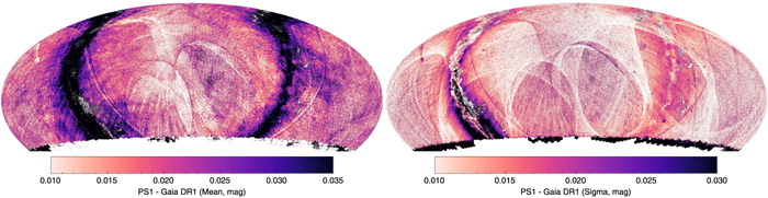
Figure 14. Comparison with Gaia DR1 photometry (see Section 7.2 for sample selection). Left: mean of PS1 − Gaia DR1. Right: standard deviation of PS1 − Gaia DR1. For pixels with  and δ > −30°, the standard deviation of the PS1 − Gaia DR1 mean values is 6.9 mmag, while the median of the standard deviations is 12.4 mmag. The former is a statement about the consistency of the Gaia DR1 and Pan-STARRS 1 photometry, while the latter reflects the combined bright-end errors for both systems.
Download figure:
Standard image High-resolution imageFor Figure 14, we calculate the difference between the estimated G-band magnitude based on PS1 g, r, i photometry and the G-band photometry reported by Gaia. For each pixel, we determine the histogram of these differences and calculate the median and the 68th percentile range. In Figure 14, these values are plotted as a color scale.
The Galactic plane is clearly poorly matched between the two photometry systems. This may in part be due to the difficulty of predicting G-band magnitudes for stars that are significantly extincted: the G band includes significant flux from the PS1 z band, which was not used in our transformation. Many other large-scale features in the median differences have structures similar to the Gaia scanning pattern (large arcs and long parallel lines). There are also structures related to the PS1 exposure footprint. These show up as a mottling on the ≈3° scale (e.g., lower right below the Galactic plane). The amplitude of the residual structures is fairly modest. The standard deviation of the median difference values is 7 mmag. This number gives an indication of the overall photometric consistency of both Gaia and PS1 and implies that the systematic error floor for each survey is less than 7 mmag.
Figure 15 shows a comparison between the Pan-STARRS mean astrometry positions in α, δ and the Gaia DR1 astrometry. For this comparison, we have selected all PS1 stars with Gaia measurements with 14 <  < 19 and with at least 10 total measurements. For Figure 15, we calculate the difference between the position predicted by PS1 at the Gaia DR1 epoch (using the proper motion and parallax fit) and the position reported by Gaia. For each pixel, we determine the histogram of these differences in the R.A. and decl. directions, and calculate the median and the 68th percentile range. In Figure 15, these values are plotted as a color scale.

Figure 15. Comparison with Gaia astrometry. Left: mean of PS1 − Gaia DR1, Right: standard deviation of PS1 − Gaia DR1. The median value of the standard deviations is (σα , σδ ) = (4.8, 3.1) mas.
Download figure:
Standard image High-resolution imageThere is good consistency between the PS1 and Gaia DR1 astrometry. There are patterns from the Galactic plane (though not very strongly at the bulge). There are also clear features due to the PS1 exposure footprint (ring structure on ≈3 degree scales). In the plots of the scatter, there are patterns that are related to the Gaia scanning rule. These are presumably regions with relatively low signal to noise in Gaia; they were also apparent in the plots of the statistics of the per-exposure measurement residuals (Figure 11). The standard deviations of the median differences are (σα , σδ ) = (4.8, 3.1) mas.
For a future data release, we will recalibrate the Pan-STARRS 3π astrometry using the Gaia DR2 release (Gaia Collaboration et al. 2018). The addition of Gaia-measured proper motions will obviate the need to correct for the Galactic rotation.
8. Polar Astrometry Issues
Internal consistency testing of the PV3 stack measurements indicated potential problems with the astrometric registration of the exposures in small areas near the North Pole. These issues were originally suggested by a few high-latitude sources with significant differences in morphology or position across bands, including strong (and anomalous) apparent color gradients. Direct investigation of a few of these anomalous sources demonstrated the presence of significant misalignments between exposures; one of the worst cases is shown in Figure 16. While such sources appeared to be rare, astrometric registration errors have the potential to affect several different source properties: morphology and photometry in addition to astrometry. Therefore, we carried out an astrometric registration test for all skycells north of δ = +70°.
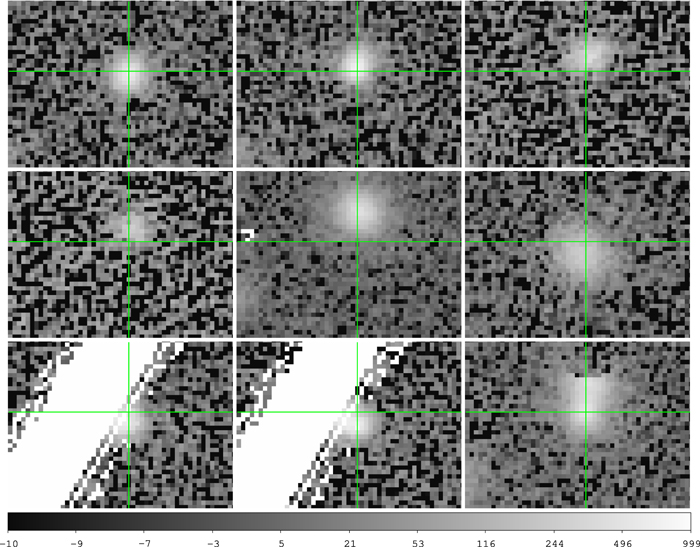
Figure 16. Example of a stack source badly affected by polar astrometry failures. Source from multiple detections from skycell 2643.093.
Download figure:
Standard image High-resolution imageThis test was based primarily on the "original detection positions," i.e., the positions of detections found in individual exposures as measured after each exposure's astrometric calibration, but before recalibration of the combined values to the Gaia reference frame (described in Section 7.2) because that step had the opportunity to repair any astrometric failures. We started by collecting the original detection positions (as defined above) for each skycell. To ensure good signal-to-noise ratios and minimize potential spurious detections, we used only the top quartile (in flux) of detections within each chip. We grouped these detections on a filter-by-filter basis within a radius of 25 (10 pixels), ensuring that each group contained only one source per exposure and retaining only groups with at least five detections; we then recorded the 2D position dispersion for each group. The mean positions for each group were cross-correlated against the Gaia DR2 sources (Gaia Collaboration et al. 2018), showing that these were real sources and providing information on their absolute astrometry.
Overall, the vast majority of the detection groups thus defined have good consistency between source positions, resulting in an astrometric dispersion of 1 pixel or less. A few "bad" groups, defined as having an internal dispersion >1 pixel, can result from spurious sources or other anomalies and are generally rare (fewer than a few percent of all groups). However, some skycells have a significant fraction (>10% of bad groups). Direct inspection demonstrates that the incidence of bad groups is related to astrometric registration failures.
Bad skycells, defined as those with more than 10% bad groups, are essentially limited to the north polar cap (δ > +80°). Of the 2500 skycells in this region, 164, or 6.6%, have more than 10% bad groups; 64 of these have more than 20% bad groups. By comparison, essentially no skycells between +70° and +80° have more than 10% bad groups. Figure 17 shows a histogram of the fraction of bad groups for each skycell.
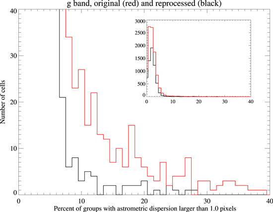
Figure 17. Histogram of the fraction of bad groups for each skycell (red line).
Download figure:
Standard image High-resolution image
In order to have an independent validation of the impact of this astrometric alignment issue, we also carried out a photometric test based on a comparison between stack and mean object photometry. In the presence of modest registration errors, mean object photometry would not be affected, as individual detection would have the correct signal, and averaging their flux in catalog space would yield the correct total magnitude. On the other hand, imperfect stacking would result in a dilution of the total signal on a pixel-by-pixel basis and result in potentially larger estimated sizes and smaller total flux for stack sources. Indeed, mean magnitudes are brighter than stack magnitudes for a significant fraction of the sources in the same skycells that are identified as bad by the relative astrometry test. Therefore, we confirm that the astrometric registration issues result in poor stack photometry for the affected skycells.
Further investigation revealed that the cause of these failures was an error in the internal reference catalog used for the PV3 analysis (see Section 3.2). This reference catalog used PS1 observations to generate a catalog of  ,
,  ,
,  ,
,  ,
,  photometry tied to the 2MASS astrometric system. The astrometry used for this catalog was generated using the analysis discussed in Section 6 to define a collection of reference stars with a coordinate system tied to 2MASS but with the higher accuracy of the Pan-STARRS measurements on small spatial scales. Unfortunately, in the vicinity of the celestial north pole, this reference catalog was contaminated by a number of poor measurements. In this portion of the sky, the astrometric registration of the exposures is more challenging due to the degeneracy between boresite position errors and field rotation. In addition, the PS1 telescope suffers from larger pointing errors near the celestial north pole, largely for the same reason. Because of these two factors, a number of exposures near the celestial pole were included in the reference database with invalid astrometry, injecting apparently good reference stars in the database with positions displaced from the true position by 1''–2''. Sometimes a chip processed in this region would find an astrometric solution using only good reference stars. Sometimes the solution would use only bad reference stars, resulting in a chip apparently displaced from the true position by 1''–2''.
To correct the astrometry failures that caused the original errors in the reference catalog, we extended the field rotation search range for the polar exposures. We also added tests to the analysis of the exposures to ensure they would not fail in a marginal way and introduce poor solutions into the calibration database. We then ran a test to confirm that we could generate good astrometry in this region with an acceptable reference catalog.
We first used the PV3 mean astrometry and photometry to define a new reference catalog in the assumption that the bulk of the failures would be eliminated by the astrometric recalibration. We reprocessed a section of the polar cap data using this PV3-based reference catalog and reran the astrometric registration test on the reprocessed exposures. The reprocessing greatly ameliorated the registration issue, as shown in Figure 17. Here, the red line shows the histogram of the fraction of bad groups for each skycell before reprocessing, while the black line refers to the results after reprocessing. The improvement is apparent. After reprocessing, only 23 cells, instead of the original 164, exceed 10% of bad groups, and even for these the fraction of bad groups is substantially reduced.
To further improve the astrometric calibration reliability in this region, we have generated a new reference catalog combining the PS1 PV3 photometry with astrometry from Gaia DR2 (Gaia Collaboration et al. 2018). We are reprocessing all images from the region north of +70° and will provide a complete Polar Region release using the same data as used for DR2. This updated release is expected to be available from MAST near the end of summer 2019.
We consider skycells with more than 10% bad groups to have been adversely affected by this problem. Users of DR2 should be aware that the affected stack skycells have poor astrometry and effective image quality. However, as these images may be useful to the community, they are available from the MAST cutout server. Users who attempt to download these problem skycells will see a warning message and should only use the skycell images for quantitative measurements with extreme caution. Because stack measurements from these skycells are significantly damaged, the DR2 release has set the measured stack properties of these objects to a null value. Again, users should exercise caution with sources from the affected skycells.
9. Conclusion
The Pan-STARRS DR2 provides astrometry and photometry of roughly 3 billion astronomical objects across the 3π Survey region. The photometry system has been shown to be reliable across the sky at the level of (8.0, 7.0, 9.0, 10.7, 12.4) mmag in ( ,
,  ,
,  ,
,  ,
,  ). The median value of the measure standard deviations for stars across the sky is (σg
, σr
, σi
, σz
, σy
) = (14, 14, 15, 15, 18) mmag, reflecting the systematic floor on the accuracy of individual measurements of bright stars. The astrometric calibration is tied to the Gaia DR1 frame with a systematic error floor of (σα
, σδ
) = (4.8, 3.1) mas. The median residual astrometric scatter for bright objects across the sky is 16 mas in both R.A. and decl. Caution should be used for 164 skycells in the celestial north pole regions where the reference catalog was contaminated with astrometric failures. The Pan-STARRS DR2 photometry and astrometry will be a valuable resource for many years for the astronomical community.
). The median value of the measure standard deviations for stars across the sky is (σg
, σr
, σi
, σz
, σy
) = (14, 14, 15, 15, 18) mmag, reflecting the systematic floor on the accuracy of individual measurements of bright stars. The astrometric calibration is tied to the Gaia DR1 frame with a systematic error floor of (σα
, σδ
) = (4.8, 3.1) mas. The median residual astrometric scatter for bright objects across the sky is 16 mas in both R.A. and decl. Caution should be used for 164 skycells in the celestial north pole regions where the reference catalog was contaminated with astrometric failures. The Pan-STARRS DR2 photometry and astrometry will be a valuable resource for many years for the astronomical community.
The past three decades have seen the digital release of a series of large-scale optical and near-IR astronomical surveys with generally steady improvements in quality. The trend begins in the mid-1990s with the digitized photographic plate surveys such as USNO-B (Monet et al. 2003) and SuperCOSMOS (Hambly et al. 2001), which have photometric errors of roughly 300 mmag and astrometric errors of roughly 200 mas. The Hipparcos and Tycho catalogs released in the mid 1990s have much smaller astrometric errors (roughly 0.6 mas) but substantially limited depth (V < 11.5) compared to the ground-based work (Hoeg et al. 1997).
The first generation of sky surveys using digital detectors, including SDSS (Lupton et al. 2001) and 2MASS (Skrutskie et al. 2006), brought a substantial leap in the quality of both photometry and astrometry along with improvements in the depth and wavelength coverage. Glossing over the details of how exactly to determine the accuracy of the SDSS and 2MASS photometry, it is clear that the photometric accuracy of those surveys are in the vicinity of 10–20 mmag for all filters, more than an order of magnitude improvement over the photographic plate surveys. The astrometric accuracy of these two surveys (roughly 50–80 mas) is also a large improvement.
The Pan-STARRS 3π Survey public release represents an important step in the ongoing progress toward covering the sky with well-characterized measurements. The nearly coincident data releases from Gaia (Lindegren et al. 2016; Gaia Collaboration et al. 2018) complement the PS1 releases greatly. In the south, the Dark Energy Survey has produced its first public data release covering roughly 5000 square degrees of the sky (Abbott et al. 2018) with reported photometric precision of better than 10 mmag.
The next decade will see further advances in survey breadth and depth along with further improvements in calibration quality. Over the next 2–3 yr, the Ultraviolet Near-Infrared Optical Northern Sky (UNIONS) Survey collaboration (a metacollaboration of the Pan-STARRS and Canada-France Imaging Survey, or CFIS, collaborations) is expected to release deep photometry in the ugriz bands for roughly 5000 deg2 of the northern hemisphere with aggressive photometric precision goals. This collaboration is in part motivated to support the Euclid satellite mission, which requires deep eight-band photometry to measure photometric redshifts but only provides the JHK bands. The Large Synoptic Survey Telescope is also expected to produce high-precision photometry and astrometry to great depths over a very large portion of the sky available from the southern hemisphere.
From our experience with the Pan-STARRS survey, and the results of the comparisons between surveys, a few lessons stand out.
First, systematic errors come in many forms and dominate the calibration precision. Internal or relative examination of the data can reveal important and unexpected effects such as the Koppenhöfer and vertical diffusion effects we identified in the Pan-STARRS devices.
Second, cross-comparisons between independent data sets are critical to reveal the limitations. This lesson has appeared several times in our investigations, in the comparison between Pan-STARRS and Gaia above, between Pan-STARRS and SDSS (Finkbeiner et al. 2016), and in the comparison between Pan-STARRS and 2MASS (Magnier et al. 2013). The cross-comparison can be used to explicitly constrain the calibration on one survey based on another, as was done by Finkbeiner et al. (2016) for the SDSS hypercalibration solution. Alternatively, the cross-comparison can be used to identify issues that may be solved by improved internal analysis.
The third lesson we have learned is that there is no substitute for photometric conditions. The cross-comparison of photometry between Pan-STARRS and Gaia suggests that the current Pan-STARRS calibration is limited in part by the excessive contribution of nonphotometric observations. This can be seen in the elevated scatter in patches that correspond to single observing blocks (see Figure 4 and discussion in Section 5.5). A future reanalysis of the Pan-STARRS data set will attempt to further limit the impact of the nonphotometric data on the photometric calibration. The other critical improvement will be to include more data from the continuing observations to ensure every patch of the sky is covered with photometric observations.
Finally, while the systematics are still probably the limiting factor for the average calibration, for individual measurements of objects, we believe our current limitations come from a few specific factors. First, the quality of the aperture corrections, especially in the ability of the software to avoid extremely deviant results on occasion appears to be one of the main drivers of bad photometry measurements for brighter stars. Second, the quality of the background sky model currently appears to be the limitation for the faint sources. Finally, improvements to the PSF model, especially including color-dependent and nonlinear effects such as the brighter-fatter effect (Antilogus et al. 2014; Gruen et al. 2015) will probably be necessary to push the limits of photometric and astrometric accuracy.
While there is clearly still room for improvement, the Pan-STARRS 3π Survey DR1 and DR2 photometry will be a critical resource for many years. We are confident that, in addition to the many science discoveries enabled by the large and accurate photometry, the high-quality photometry provided here will save observers countless hours of telescope time by obviating, or at least greatly reducing, the need to observe standard stars on a regular basis.
The Pan-STARRS1 Surveys (PS1) have been made possible through contributions of the Institute for Astronomy, the University of Hawaii, the Pan-STARRS Project Office, the Max-Planck Society and its participating institutes, the Max Planck Institute for Astronomy, Heidelberg, and the Max Planck Institute for Extraterrestrial Physics, Garching, The Johns Hopkins University, Durham University, the University of Edinburgh, Queen's University Belfast, the Harvard-Smithsonian Center for Astrophysics, the Las Cumbres Observatory Global Telescope Network Incorporated, the National Central University of Taiwan, the Space Telescope Science Institute, the National Aeronautics and Space Administration under grant No. NNX08AR22G issued through the Planetary Science Division of the NASA Science Mission Directorate, the National Science Foundation under grant No. AST-1238877, the University of Maryland, and Eötvös Loránd University (ELTE) and the Los Alamos National Laboratory. E.A.M. is also supported for portions of this work by National Science Foundation grant No. AST-1313455. Color maps for Figures 2, 4, 5, 9, 10, 11, and 12 are based on the matplotlib "magma" color map with additional guidance from Peter Kovesi's work (Good Colour Maps: How to Design Them; Kovesi 2015).