


Abstract
Over 3 billion astronomical sources have been detected in the more than 22 million orthogonal transfer CCD images obtained as part of the Pan-STARRS1 3π survey. Over 85 billion instances of those sources have been automatically detected and characterized by the Pan-STARRS Image Processing Pipeline photometry software, psphot. This fast, automatic, and reliable software was developed for the Pan-STARRS project but is easily adaptable to images from other telescopes. We describe the analysis of the astronomical sources by psphot in general as well as for the specific case of the third processing version used for the first two public releases of the Pan-STARRS 3π Survey data.
Export citation and abstract BibTeX RIS
1. Introduction
The 1.8 m Pan-STARRS1 telescope (PS1) is located on the summit of Haleakala on the Hawaiian island of Maui. The wide-field optical design of the telescope (Hodapp et al. 2004) produces a 33 field of view with low distortion and minimal vignetting even at the edges of the illuminated region. The optics and natural seeing combine to yield good image quality: 75% of the images have FWHM values less than (151, 139, 134, 127, 121) for ( ,
,  ,
,  ,
,  ,
,  ), with a floor of ∼07.
The Pan-STARRS1 camera (Tonry & Onaka 2009), known as GPC1, consists of a mosaic of 60 back-illuminated CCDs manufactured by Lincoln Laboratory. The CCDs each consist of an 8 × 8 grid of 590 × 598 pixel readout regions, yielding an effective 4846 × 4868 detector. Initial performance assessments are presented in Onaka et al. (2008). Routine observations are conducted remotely from the Advanced Technology Research Center in Kula, the main facility of the University of Hawaii's Institute for Astronomy (IfA) operations on Maui. The Pan-STARRS1 filters and photometric system have already been described in detail in Tonry et al. (2012).
For nearly 4 yr, from 2010 May through 2014 March, this telescope was used to perform a collection of astronomical surveys under the aegis of the Pan-STARRS Science Consortium. The majority of the time (56%) was spent on surveying the three-quarters of the sky north of −30° decl. with  ,
,  ,
,  ,
,  ,
,  filters in the so-called 3π Survey. Another
  of the time was concentrated on repeated deep observations of 10 specific fields in the Medium-Deep Survey. The rest of the time was used for several other surveys, including a search for potentially hazardous asteroids in our solar system. The details of the telescope, surveys, and resulting science publications are described by Chambers et al. (2016).
Since 2014 March, PS1 has been rededicated to a mission of searching for hazardous asteroids, funded by the NASA NEO Program. Additional partners collaborate with the Pan-STARRS team to harvest the transient sources such supernovae and gravitational wave counterparts. A second Pan-STARRS telescope (PS2; Chambers et al. 2016, K. C. Chambers et al. 2020, in preparation), generally matching the PS1 design (Morgan et al. 2012) has since been constructed and has been producing science results since early 2018.
Pan-STARRS produced its first large-scale public data release, Data Release 1 (DR1), on 2016 December 16. DR1 contains the results of the third full reduction of the Pan-STARRS 3π Survey archival data, identified as PV3. Previous reductions (PV0, PV1, and PV2; see Magnier et al. 2020a) were used internally for pipeline optimization and the development of the initial photometric and astrometric reference catalog (Magnier et al. 2020b). The products from these reductions were not publicly released but have been used to produce a wide range of scientific papers from the Pan-STARRS1 Science Consortium members (Chambers et al. 2016). DR1 contained only average information resulting from the many individual images obtained by the 3π Survey observations. A second data release, DR2, was made available 2019 January 28. DR2 provides measurements from all of the individual exposures and includes improved astrometric calibration as well as improvements to the photometric calibration of the stack and "forced-warp" measurements from the PV3 processing of that data set.
The Pan-STARRS public data releases are hosted by the Barbara A. Mikulski Archive for Space Telescopes (MAST) at the Space Telescope Science Institute. MAST provides access to the image data products and a hierarchical database of measurements using a system developed specifically for the Pan-STARRS data set. Development of this database system was the product of a collaboration between the Pan-STARRS Project and Alex Szalay's database development group at The Johns Hopkins University (JHU; Heasley 2008). The resulting system, called the Published Science Products Subsystem, or PSPS (Heasley et al. 2006), was initially used within the Pan-STARRS Science Consortium for large-scale data access. A duplicate PSPS installation was created at MAST for the DR1 and DR2 public releases.
This is the fourth in a series of seven papers describing the Pan-STARRS1 Surveys, the data reduction techniques, and the resulting data products. This paper (Paper IV) describes the details of the source detection and photometry, including point-spread-function (PSF) and extended source model fitting, and the techniques for "forced" photometry measurements. The same analysis software, called psphot, is used for individual images, image stacks, and difference images. The software described here was used with a single consistent set of parameters for the complete PV3 analysis, used for both DR1 and DR2. The software was also used for the analysis of the Medium-Deep Survey data, though with a different software version and some modifications of the analysis parameters to better suit the longer exposures. This program as well as the rest of the Pan-STARRS Image Processing Pipeline (IPP) software suite is available for download from http://ipp.ifa.hawaii.edu.
Chambers et al. (2016, Paper I) provide an overview of the Pan-STARRS System, the design and execution of the Surveys, the resulting image and catalog data products, a discussion of the overall data quality and basic characteristics, and a brief summary of important results.
Magnier et al. (2020a, Paper II) describe how the various data processing stages are organized and implemented in the Image Processing Pipeline (IPP), including details of the processing database, which is a critical element in the IPP infrastructure.
Waters et al. (2020, Paper III) describe the details of the pixel processing algorithms, including detrending, warping, and adding (to create stacked images) and subtracting (to create difference images), and the resulting image products and their properties.
Magnier et al. (2020b, Paper V) describe the final calibration process and the resulting photometric and astrometric quality.
Flewelling et al. (2020, Paper VI) describe the details of the resulting catalog data and its organization in the Pan-STARRS database system, PSPS.
M. Huber et al. (2020, in preparation) describe the Medium-Deep Survey in detail, including the unique issues and data products specific to that survey. The Medium-Deep Survey is not part of DRs 1 or 2 and will be made available in a future data release.
In this article, we use the following typefaces to distinguish different concepts:
- 1.Small caps for the analysis stages.
- 2.Italics for database tables and columns.
- 3.Fixed-width font for program names, variables, and miscellaneous constants.
The latter category includes a number of configuration parameters used to define the psphot analysis. In those cases, unless the values used for the PV3 analysis are explicitly discussed, we include the PV3 value immediately after the configuration variable name in parentheses.
2. Background
The photometric and astrometric precision goals for the Pan-STARRS1 surveys were quite stringent. The astrometric goals were relative astrometric accuracy of 10 mas and absolute astrometric accuracy of 100 mas with respect to the ICRS reference stars. For photometry, the goal was 10 mmag accuracy within the internal photometric system across the sky, though the tie to an absolute standard was not required to meet this standard.
An additional constraint on the Pan-STARRS analysis system comes from the high data rate. PS1 produces typically ∼500 exposures per night, corresponding to ∼750 billion pixels of imaging data. The images range from high galactic latitudes to the Galactic bulge, so large numbers of measurable stars can be expected in much of the data. The combination of the high precision goals of the astrometric and photometric measurements and the high data rate (and a finite computing budget) means that the process of detecting, classifying, and measuring the astronomical sources in the image data stream in a timely fashion are a significant challenge.
In order to achieve these ambitious goals, the source detection, classification, and measurement process must be both precise and efficient. Not only is it necessary to make a careful measurement of the flux of individual sources, it is also critical to characterize the image PSF and its variations across the field and from image to image. Because comparisons between images must be reliable, the measurements must be stable for both photometry and astrometry.
A variety of astronomical software packages perform the basic source detection, measurement, and classification tasks needed by the Pan-STARRS IPP. Each of these programs have their own advantages and disadvantages. Below we discuss some of the most widely used of these other packages, highlighting the features of the programs that are particularly desirable and noting aspects of the programs that are problematic for the IPP.
- 1.DoPhot: analytical fitted model with aperture corrections. Pros: well-tested, stable code. Cons: limited range of models, algorithm converges slowly to a PSF model, limited tests of PSF validity, inflexible code base, Fortran (Schechter et al. 1993).
- 2.DAOPhot: pixel-map PSF model with analytical component. Pros: well-tested, high-quality photometry. Cons: difficult to use in an automated fashion; does it handle 2D variations well? (Stetson 1987).
- 3.Sextractor: pure aperture measurement with rudimentary source subtraction. Pros: fast, widely used, easy to automate. Cons: poor source separation in crowded regions, PSF modeling was only in beta, not widely used at the time (Bertin & Arnouts 1996).
- 4.galfit: detailed galaxy modeling. Not a multisource PSF analysis tool. Cons: does not provide a PSF model, not easily automated, very detailed results in very slow processing, only a galaxy analysis program (Peng et al. 2002).
- 5.SDSS phot. Cons: tightly integrated into the SDSS software environment (Lupton et al. 2001).
When the IPP development was starting, the existing photometry packages either did not meet the accuracy requirements or required too much human intervention to be considered for the needs of PS1. In the case of the SDSS photo tool, the software was judged to be too tightly integrated to the architecture of SDSS to be easily reintegrated into the Pan-STARRS pipeline. A new photometry analysis package was developed using lessons learned from the existing photometry systems. In the process, the source analysis software was written using the data analysis C-code library written for the IPP, psLib (Magnier et al. 2020a). Components of the photometry code were integrated into the IPP's midlevel astronomy data analysis toolkit called psModules (Magnier et al. 2020a). The resulting software, "psphot," can be used either as a standalone C program or as a set of library functions that may be integrated into other programs
Several variants of psphot have been used in the PS1 PV3 analysis. The main variant of psphot operates on a single image or a group of related images representing the data read from the multiple chips of a mosaic camera from a single exposure. The images are expected to have already been detrended so that pixel values are linearly related to the flux. The gain may be specified by the configuration system or a variance image may be supplied. A mask may also be supplied to mark good, bad, and suspect pixels. This variant of psphot can be called a standalone program, also called psphot. In standard IPP operations, this variant is used as a library call within the analysis program ppImage during the chip analysis stage.
In the standard IPP analysis, the initial stage of processing is performed in parallel on each of the individual CCDs in the camera. This so-called chip-stage analysis includes the detrending of the CCD image (instrumental signature removal) as well as the detection and analysis of sources in the image using the basic version of psphot. The next stage of the analysis, the camera stage, consists of photometric and astrometric calibration.
After the calibrations are available, the detrended CCD images from an entire exposure are geometrically transformed to a common pixel grid in the warp stage of the pipeline. The resulting warped images are generated on a predefined tessellation of the sky that starts with projection centers spaced roughly 4° across the sky. Around each of these projection centers, a large regular pixel grid is defined and then subdivided along pixel boundaries into smaller units that are well matched to the memory footprint of our processing computers. These smaller images, called "skycells," are defined with 1' of overlap with their neighbors so that any modest-sized object can be analyzed entirely on a single pixel grid. Note that the term skycell is used to describe the particular subdivision of the sky. A typical exposure from the GPC1 camera generates warp images on roughly 70 skycells. We refer to the specific warped images from an exposure as "warps."
Multiple warps for the same skycell are combined together in the stack stage of the IPP by coadding the flux to generate a deep "stack" image. Alternatively, one warp may be subtracted from another warp of the same skycell, or a stack image may be subtracted from a warp image, or indeed from another stack. These subtraction operations are used to detect moving and transient objects within the IPP. Different variants of psphot are used for the source detection and analysis for each of these different analysis stages.
The variant called psphotStack accepts a set of images, each representing the same patch of sky (with pixels aligned) in a different filter. This version was used in the IPP for the analysis of the deep "stacks" produced by the IPP stack stage. Nominally, the full grizy filter set was used for the analysis of the PS1 PV3 stack images, though where insufficient data were available in a given filter, a subset of these filters was processed as a group. As discussed in detail below, the psphotStack analysis includes the capability of measuring forced PSF photometry in some filter images based on the position of sources detected in the other filters. It also includes an option to convolve the set of images to a single, common PSF size across the filters for the purpose of fixed-aperture photometry.
Another variant of psphot used in the PV3 analysis is called psphotFullForce. In this variant, a set of images all representing the same coaligned pixels are processed together, with the positions of sources to be analyzed loaded from a supplied file. In this variant of the analysis, sources are not discovered—only the supplied sources are considered. PSF models are determined for each exposure, and the forced PSF photometry is measured for all sources. A subset of sources may also be used to measure forced galaxy shape parameters. As described below, a grid of galaxy models is fitted based on the supplied guess model.
3. psphot Design Goals
The top-level design goals of psphot are to detect and determine the instrumental positions and fluxes of astronomical sources in the images. For extended sources, the goals also include the measurement of a variety of morphological information, including galaxy model parameters and nonparametric measurements of the sizes and profiles of the galaxies to aid in classification and for weak lensing analysis. For trailed asteroids, the goal also includes the measurement of the length and direction of the trail.
Beyond these basic elements, psphot has a number of design goals that we believe will help make it usable in a wide range of circumstances. The critical astronomy-driven measurement goals of the Pan-STARRS project, which drive the design of psphot, are the photometric accuracy goal (10 mmag) and the relative astrometric accuracy goal (10 mas) for bright stars for which the photon shot noise is small compared to the systematic errors.
For psphot, the photometry accuracy goal implies that the measured photometry of stellar sources must be substantially better than this 10 mmag goal as the photometry error per image is combined with an error in the flat-field calibration and an error in measuring the atmospheric effects. We have set a goal for psphot of 3 mmag photometric consistency for bright stars between pairs of images obtained in photometric conditions at the same pointing, i.e., to remove sensitivity to flat-field errors. This goal splits the difference between the three main contributors and still allows some leeway. This goal must be met for well-sampled images and images with only modest undersampling.
The relative astrometric calibration depends on the consistency of the individual measurements. The measurements from psphot must be sufficiently representative of the true source position to enable astrometric calibration at the 10 mas level. The error in the individual measurements will be folded together with the errors introduced by the optical system, the effects of seeing, and the available reference catalogs. We have set a goal for psphot of 5 mas consistency between the true source position and the measured position given reasonable PSF variations under simulations. This level must be reached for images with 250 mas pixels, implying psphot must introduce measurement errors less than 1/50 of a pixel. The choice of 32 bit floating point data values for the source centroids places a numerical limit of 1 × 10⁻⁷ on the accuracy of a pixel relative to the size of a chip (because a single data value is used for X or Y). For the 48002 GPC chips, this yields a limit of about 0.25 mas.
The design goals for psphot are chosen to make the program flexible, general, and able to meet the unknown usage cases future projects may require:
- 1.Flexible PSF model. Different image sources require different ways of representing the PSF. Ideally, both analytical and pixel-based versions should be possible.
- 2.PSF spatial variation. Most images result in some spatial PSF variations at a certain level. The PSF representation should naturally incorporate 2D variations.
- 3.Flexible non-PSF models. psphot must be able to represent PSF-like sources as well as non-PSF sources (e.g., galaxies). It must be easy to add new source models as interesting representations of sources are invented.
- 4.Clean code base. psphot should incorporate a high-degree of abstraction and encapsulation so that changes to the code structure can be performed without pulling the code apart and starting from scratch.
- 5.PSF validity tests. psphot should include the ability to choose different types of PSF models for different situations, or to provide the user with methods for assessing the different PSF models.
- 6.Careful systematic corrections. psphot must carefully measure and correct for the photometric and astrometric trends introduced by using analytical PSF models.
- 7.User configurable. psphot should allow users to change the options easily and to allow different approaches to the analysis.
The success of the psphot implementation in meeting the photometry and astrometry design requirements is demonstrated by the achieved accuracy for the Pan-STARRS 3π Survey data. For a survey like the Pan-STARRS1 3π Survey to achieve photometry and astrometry accuracy at the level of our goals, not only must the measurement of the astronomical detections be precise, but it is necessary for the detrending and calibration processes to correct for a wide variety of systematic effects, and it is also necessary for the observations to be performed in such a way that the data can be calibrated well. These other aspects of the process are discussed in detail elsewhere (Papers I, III, and V). In the end, the goals were largely achieved for the Pan-STARRS1 3π Survey. As reported in Paper V, the resulting photometric system is consistent across the sky to between 7 and 12.4 mmag, depending on the filter. The systematic error floor for individual photometry measurements is  mmag. The bright-star systematic error floor for individual astrometric measurements is 16 mas and the Pan-STARRS Data Release 2 (DR2) astrometric system is tied to the Gaia DR1 (Lindegren et al. 2016) coordinate frame with a systematic uncertainty of ∼5 mas.
4. Basic Analysis
4.1. Overview
The basic psphot analysis is divided into several major stages, as listed below.
- 1.Image preparation. Load data, characterize the image background, load or construct variance and mask images.
- 2.Initial source detection. Smooth, find peaks, measure basic properties with focus on the point sources to measure the PSF.
- 3.PSF determination. Select PSF candidates, perform model fits, build PSF model from fits, select best PSF model class.
- 4.Bright-source analysis. Fit sources with PSFs, determine PSF validity, subtract PSF-like sources, fit non-PSF model(s), select best model class, subtract model.
- 5.Faint source analysis. Detect low-level sources, measure properties (aperture or PSF).
- 6.Aperture corrections.Measure the curve of growth, spatial aperture variations, and background-error corrections.
- 7.Output. Write out sources in selected format, write out difference image, variance image, etc., as selected.
In addition to this basic sequence, additional analysis steps may be performed. An "extended source" analysis mode is available to measure photometry and morphology of galaxies and other resolved sources. Forced photometry may be performed for both point-like and extended sources. A special mode is available for the photometry of sources detected in difference images. These different modes are discussed in their own sections below.
Table 1 lists the types of analyses performed by psphot, specifying which of the psphot use cases performs the given analysis. The table also provides a reference to the section of this paper in which the analysis is described. Not all analyses are relevant to all sources in all images. The table identifies those cases where the analyses are applied to only a subset of all sources.
Table 1. Measurements Performed by psphot, and Whether Performed in Each of the 4 IPP Analysis Stages
| Measurement | CHIP | STACK | FORCED WARP | DIFF | Section | Details |
|---|---|---|---|---|---|---|
| Background Subtraction | Y | Y | Y | N a | 4.3 | N/A |
| Peaks | Y | Y | N | Y | 4.4.1 | All detections |
| Footprints | Y | Y | N | Y | 4.4.2 | All detections |
| Moments | Y | Y | Y | Y | 4.4.3 | All detections |
| PSF Model | Y | Y | Y | N b | 4.5 | Selected bright stars |
| Bright-star Profile | Y | Y | N | Y | 4.6.1 | Saturated stars |
| Radial Profiles v1 | Y | Y | N | Y | 4.6.3 | All detections |
| Kron Fluxes | Y | Y | Y | Y | 4.6.4 | All detections |
| Source-size Tests | Y | Y | N | Y | 4.6.5 | All detections |
| Nonlinear PSF Fits | Y | Y | N | N | 4.6.6 | S/N > 20 |
| Unconvolved Galaxy Model | Y | Y | N | N | 4.6.8 | S/N > 20, extended |
| Unconvolved Streak Model | N | N | N | Y | 4.6.8 | S/N > 20, extended |
| Linear PSF Fits | Y | Y | Y | Y | 4.7 | All detections |
| Radial Profiles v2 | Y | Y | N | Y | 5.1 | Gal. latitude cut |
| Petrosian Fluxes | N | Y | Y | N | 5.2 | Gal. latitude cut |
| Convolved Galaxy Models | N | Y | N | N | 5.3 | Gal. latitude cut, mag cut |
| Fixed-aperture Photometry | N | Y | Y | N | 5.4 | All detections |
| Convolved, Fixed Apertures | N | Y | N | N | 5.4 | All detections |
| Aperture Corrections | Y | Y | Y | N | 4.8 | All detections |
| Forced PSF Fluxes | N | N | Y | N | 6 | All detections |
| Forced Galaxy Models | N | N | Y | N | 6.2 | Requires stack galaxy models |
| Lensing Parameters | N | Y | Y | N | 6.3 | All detections |
Notes. The analysis is described in this article in the listed sections.
a Background subtraction is performed by ppSub before calling psphot. b PSF modeling is performed by ppSub on the input warps before calling psphotDownload table as: ASCIITypeset image
psphot is highly configurable. Users may choose via the configuration system which of the above analyses are performed. This is useful for testing but also allows for specialized use cases. For example, the PSF model may already be available from external information, in which case the PSF modeling stage can be skipped.
Ultimately, all measurements of individual astronomical sources from psphot are reported in one of the tables in the PSPS database. As discussed in detail in Paper VI, measurements from individual exposures are available from the Detection table. Measurements of objects in the stacked images are stored in one of several Stack... tables, while the "forced" measurements from individual warp images are stored in tables beginning with ForcedWarp.
4.2. Informational and Warning Bit Flags
During the psphot analysis, there are a wide variety of conditions that are identified by the analysis software. As part of the output data for each detected source, two fields that encode these conditions as bit values in the two 32 bit integers are provided. The following two tables list the individual bit values in these two fields. These informational and warning bits are described in more detail later in this article.
Table 2 lists the flags recorded in the output field FLAGS. When data from psphot is loaded into a DVO database (Magnier et al. 2020b), these values are stored in the field Measure.photFlags and exposed in the public database (PSPS; Flewelling et al. 2020) in the fields Detection.infoFlag, StackObjectThin.XinfoFlag (where X is one of grizy), and ForcedWarpMeasurement.FinfoFlag. Table 3 lists the flags recorded in the output field FLAGS2. When data from psphot are loaded into a DVO database (Magnier et al. 2020b), these values are stored in the field Measure.photFlags2, and they are exposed in PSPS in the fields Detection.infoFlag2, StackObjectThin.XinfoFlag2 (where X is one of grizy), and ForcedWarpMeasurement.FinfoFlag2.
Table 2. Detection Flag Values #1 Reported by psphot
| Flag Name | Flag Value | Description |
|---|---|---|
| PM_SOURCE_MODE_PSFMODEL | 0x00000001 | Source fitted with a PSF model (linear or nonlinear) |
| PM_SOURCE_MODE_EXTMODEL | 0x00000002 | Source fitted with an extended source model |
| PM_SOURCE_MODE_FITTED | 0x00000004 | Source fitted with nonlinear model (PSF or EXT; good or bad) |
| PM_SOURCE_MODE_FAIL | 0x00000008 | Fit (nonlinear) failed (nonconverge, off-edge, run to zero) |
| PM_SOURCE_MODE_POOR | 0x00000010 | Fit succeeds, but low-S/N or high chi-square |
| PM_SOURCE_MODE_PAIR | 0x00000020 | Source fitted with a double PSF |
| PM_SOURCE_MODE_PSFSTAR | 0x00000040 | Source used to define PSF model |
| PM_SOURCE_MODE_SATSTAR | 0x00000080 | Source model peak is above saturation |
| PM_SOURCE_MODE_BLEND | 0x00000100 | Source is a blend with other sources a |
| PM_SOURCE_MODE_EXTERNAL | 0x00000200 | Source based on supplied input position |
| PM_SOURCE_MODE_BADPSF | 0x00000400 | Failed to get good estimate of object's PSF |
| PM_SOURCE_MODE_DEFECT | 0x00000800 | Source is thought to be a defect |
| PM_SOURCE_MODE_SATURATED | 0x00001000 | Source is thought to be saturated pixels (bleed trail) |
| PM_SOURCE_MODE_CR_LIMIT | 0x00002000 | Source has crNsigma above limit |
| PM_SOURCE_MODE_EXT_LIMIT | 0x00004000 | Source has extNsigma above limit |
| PM_SOURCE_MODE_MOMENTS_FAILURE | 0x00008000 | Could not measure the moments |
| PM_SOURCE_MODE_SKY_FAILURE | 0x00010000 | Could not measure the local sky |
| PM_SOURCE_MODE_SKYVAR_FAILURE | 0x00020000 | Could not measure the local sky variance |
| PM_SOURCE_MODE_BELOW_MOMENTS_SN | 0x00040000 | Moments not measured due to low S/N. a |
| PM_SOURCE_MODE_BIG_RADIUS | 0x00100000 | Poor moments for small radius, try large radius |
| PM_SOURCE_MODE_AP_MAGS | 0x00200000 | Source has an aperture magnitude |
| PM_SOURCE_MODE_BLEND_FIT | 0x00400000 | Source was fitted as a blend |
| PM_SOURCE_MODE_EXTENDED_FIT | 0x00800000 | Full extended fit was used |
| PM_SOURCE_MODE_EXTENDED_STATS | 0x01000000 | Extended aperture stats calculated |
| PM_SOURCE_MODE_LINEAR_FIT | 0x02000000 | Source fitted with the linear fit |
| PM_SOURCE_MODE_NONLINEAR_FIT | 0x04000000 | Source fitted with the nonlinear fit |
| PM_SOURCE_MODE_RADIAL_FLUX | 0x08000000 | Radial flux measurements calculated |
| PM_SOURCE_MODE_SIZE_SKIPPED | 0x10000000 | Size could not be determined a |
| PM_SOURCE_MODE_ON_SPIKE | 0x20000000 | Peak lands on diffraction spike |
| PM_SOURCE_MODE_ON_GHOST | 0x40000000 | Peak lands on ghost or glint |
| PM_SOURCE_MODE_OFF_CHIP | 0x80000000 | Peak lands off edge of chip |
Notes. These are saved in output catalogs as the field FLAGS, in the DVO database as Measure.photFlags, and in the public database as Detection.infoFlag, StackObjectThin.XinfoFlag (where X is one of grizy), and ForcedWarpMeasurement.FinfoFlag.
a Not used for DR1 or DR2.Download table as: ASCIITypeset image
Table 3. Detection Flag Values #2 Reported by psphot
| Flag Name | Flag Value | Description |
|---|---|---|
| PM_SOURCE_MODE2_DIFF_WITH_SINGLE | 0x00000001 | Diff source matched to a single positive detection |
| PM_SOURCE_MODE2_DIFF_WITH_DOUBLE | 0x00000002 | Diff source matched to positive detections in both images |
| PM_SOURCE_MODE2_MATCHED | 0x00000004 | Source generated based on another image |
| PM_SOURCE_MODE2_ON_SPIKE | 0x00000008 |
 of (PSF-weighted) pixels land on diffraction spike of (PSF-weighted) pixels land on diffraction spike |
| PM_SOURCE_MODE2_ON_STARCORE | 0x00000010 |
 of (PSF-weighted) pixels land on star core of (PSF-weighted) pixels land on star core |
| PM_SOURCE_MODE2_ON_BURNTOOL | 0x00000020 |
 of (PSF-weighted) pixels land on burntool of (PSF-weighted) pixels land on burntool |
| PM_SOURCE_MODE2_ON_CONVPOOR | 0x00000040 |
 of (PSF-weighted) pixels land on convpoor of (PSF-weighted) pixels land on convpoor |
| PM_SOURCE_MODE2_PASS1_SRC | 0x00000080 | Source detected in first pass analysis |
| PM_SOURCE_MODE2_HAS_BRIGHTER_NEIGHBOR | 0x00000100 | Peak is not the brightest in its footprint |
| PM_SOURCE_MODE2_BRIGHT_NEIGHBOR_1 | 0x00000200 |
|
| PM_SOURCE_MODE2_BRIGHT_NEIGHBOR_10 | 0x00000400 |
|
| PM_SOURCE_MODE2_DIFF_SELF_MATCH | 0x00000800 | Positive detection match is probably this source |
| PM_SOURCE_MODE2_SATSTAR_PROFILE | 0x00001000 | Saturated source is modeled with a radial profile |
| PM_SOURCE_MODE2_ECONTOUR_FEW_PTS | 0x00002000 | Too few points to measure the elliptical contour |
| PM_SOURCE_MODE2_RADBIN_NAN_CENTER | 0x00004000 | Radial bins failed with too many NaN center bin |
| PM_SOURCE_MODE2_PETRO_NAN_CENTER | 0x00008000 | Petrosian radial bins failed with too many NaN center bin a |
| PM_SOURCE_MODE2_PETRO_NO_PROFILE | 0x00010000 | Petrosian not built because radial bins missing |
| PM_SOURCE_MODE2_PETRO_INSIG_RATIO | 0x00020000 | Insignificant measurement of Petrosian ratio |
| PM_SOURCE_MODE2_PETRO_RATIO_ZEROBIN | 0x00040000 | Petrosian ratio in the zeroth bin (likely bad) |
| PM_SOURCE_MODE2_EXT_FITS_RUN | 0x00080000 | We attempted to run extended fits on this source |
| PM_SOURCE_MODE2_EXT_FITS_FAIL | 0x00100000 | At least one of the model fits failed |
| PM_SOURCE_MODE2_EXT_FITS_RETRY | 0x00200000 | Trailed asteroid model fit was retried with new window |
| PM_SOURCE_MODE2_EXT_FITS_NONE | 0x00400000 | All of the model fits failed |
Notes. These are saved in output catalogs as the field FLAGS2, in the DVO database as Measure.photFlags2, and in the public database as Detection.infoFlag2, StackObjectThin.XinfoFlag2 (where X is one of grizy), and ForcedWarpMeasurement.FinfoFlag2.
a Not used for DR1 or DR2.Download table as: ASCIITypeset image
4.3. Image Preparation
The first step is to prepare the image for detection of the astronomical sources. We need three separate images: the measured flux (signal image), the corresponding variance image, and a mask defining which pixels are valid and which should be ignored. The signal and variance images are represented internally as 32 bit floating point values. The variance and mask images may either be provided by the user, or they may be automatically generated from the input image, based on configuration-defined values for the image gain, read noise, saturation, and so forth. Within the IPP analysis, we normally use images that are equivalent to the digital numbers (scaled by the detrend images), but as long as the variance image is constructed in a consistent fashion, psphot can use images in electron, calibrated flux units, or other conventions (though this would require some tuning of configuration parameters). For the function-call form of the program, the flux image is provided in the API, and references to the mask and variance are provided in the configuration information. As in the standalone C program, the variance and mask may be constructed automatically by psphot.
The mask is represented as a 16 bit integer image in which a value of 0 represents a valid pixel. Each of the 16 bits define different reasons a pixel should be ignored, listed in Table 4. This allows us to optionally respect or ignore the mask depending on the circumstance. For example, in some cases, we ignore saturated pixels completely while in other circumstances, it may be useful to know the flux value of the saturated pixel. In addition, the mask pixels are used to define the pixels available during a model fit; those which should be ignored for that specific fit are "marked" by setting a special bit (MARK=0x8000). The initial mask, if not supplied by the user or library calls, is constructed by default from the image by applying three rules: (1) Pixels that are above a specified saturation level are marked as saturated. The level is specified by the camera format keyword CELL.SATURATION, which may specify a value or define a header keyword which in turn specifies the value in the image header. In the case of PS1 PV3, the header keyword MAXLIN specifies the saturation level for each chip (see Waters et al. 2020). (2) Pixels that are below a user-defined value (CELL.BAD = 0 for PV3) are considered unresponsive and masked as dead. (3) Pixels that lie outside of a user-defined coordinate window are considered nondata pixels (e.g., overscan) and are marked as invalid. (psphot recipe keywords XMIN, XMAX, YMIN, YMAX, all set to 0 for PS1 PV3—invalid pixels were specified for PS1 PV3 with a supplied mask image (see Waters et al. 2020).
Table 4. Pixel Values for Input GPC1 Mask Images Used by psphot
| Mask Name | Mask Value | Dynamic? | Suspect? | Description |
|---|---|---|---|---|
| DETECTOR | 0x0001 | N | N | A detector defect is present. |
| FLAT | 0x0002 | N | N | The flat-field model does not calibrate the pixel reliably. |
| DARK | 0x0004 | N | N | The dark model does not calibrate the pixel reliably. |
| BLANK | 0x0008 | N | N | The pixel does not contain valid data. |
| CTE | 0x0010 | N | N | The pixel has poor charge transfer efficiency. |
| SAT | 0x0020 | Y | N | The pixel is saturated. |
| LOW | 0x0040 | Y | N | The pixel has a lower value than expected. |
| SUSPECT | 0x0080 | Y | Y | The pixel is suspected of being bad a . |
| BURNTOOL | 0x0080 | Y | Y | The pixel contains a burntool-repaired streak. |
| CR | 0x0100 | Y | N | A cosmic ray is present. |
| SPIKE | 0x0200 | Y | Y | A diffraction spike is present. |
| GHOST | 0x0400 | Y | Y | An optical ghost is present. |
| STREAK | 0x0800 | Y | Y | A streak is present. |
| STARCORE | 0x1000 | Y | Y | A bright star core is present. |
| CONV.BAD | 0x2000 | Y | N | The pixel is bad after convolution with a bad pixel. |
| CONV.POOR | 0x4000 | Y | Y | The pixel is poor after convolution with a bad pixel. |
| MARK | 0x8000 | X | X | An internal flag for temporarily marking a pixel. |
Notes. The table gives the bit value used to mark the listed effects. Bits marked as "dynamic" are set for each image based on the contents, such as the locations of bright stars. Bits marked as "suspect" represent effects that do not definitely affect the photometry, but users should be careful. The mask image headers also list these values.
a The SUSPECT bit is generic and only used if a specific reason cannot be identified. It is overloaded on the same bit as BURNTOOL.Download table as: ASCIITypeset image
The library functions used by psphot understand two types of masked pixels: "bad" and "suspect." Bad pixels are those that should not be used in any operations, while suspect pixels are those for which the reported signal may be contaminated or biased, but may be usable in some contexts. For example, a pixel with poor charge transfer efficiency is likely to be too untrustworthy to use in any circumstance, while a pixel in which persistence ghosts have been subtracted might be useful for detection or even analysis of brighter sources. Table 4 lists the 16 bit values used for PS1 mask images, along with their description (see Waters et al. 2020 for additional information).
An important point to note is that psphot does not attempt to interpolate or replace bad pixel values in the images before processing. The GPC1 images have quite extensive masking due to both defects and natural gaps between detectors and amplifier regions. On average, roughly 71% of the full usable field of view is covered with valid pixels (see Paper III for more discussion). Any attempt to interpolate bad pixels would be quickly overwhelmed by these extensive regions. Rather than attempt to fill in the bad pixels, we rely in the PS1 PV3 processing on the fact that regions on the sky were observed many times. Thus, it should be noted that model-fitting measurements (which can naturally ignore masked pixels) should generally be more reliable than aperture-like measurements for single exposures. Aperture-like measurements from the stacks do not suffer from this masking issue. See also the discussion of the PSF_QF and PSF_QF_PERFECT parameters for judging the impact of masking on a particular source (Section 4.5.3).
The variance image, if not supplied, is constructed by default from the flux image using the configuration supplied gain and read noise values to calculate the appropriate Poisson statistics for each pixel. The parameters are determined based on the camera format keywords CELL.GAIN and CELL.READNOISE, which in the case of PS1 PV3 refer to the header keywords GAIN and RDNOISE. In this case, the image is assumed to represent the readout from a single detector, with well-defined gain and read-noise characteristics. This assumption is not always valid. For example, if the input flux image is the result of an image stack with a variable number of input measurements per pixel (due to masking and dithering), the variance cannot be calculated from the signal image alone. It is necessary in such a case to supply a variance image that accurately represents the variance as a function of position in the image.
Some image processing steps introduce cross-correlation between pixel fluxes. An obvious case is smoothing, but geometric transformations that redistribute fractional flux between neighboring pixels also introduces cross-correlations. In the noise model, it is necessary to track the impact of the cross-correlations on the per-pixel variance. In the general case, this would require a complete covariance image, consisting of the set of cross-correlated pixels for each image pixel. Because a typical smoothing or warping operation may introduce correlation between 25 and 100 neighboring pixels, the size of such a covariance image is prohibitive.
Before sources are detected in the image, a model of the background is subtracted. The image is divided into a grid of background points with a spacing defined by the psphot recipe values BACKGROUND.XBIN, BACKGROUND.YBIN, set to 400 pixels (∼100'') for PV3. Superpixels of size BACKGROUND.XSAMPLE, BACKGROUND.YSAMPLE (2 × 2 for PV3) times larger than this spacing are used to measure the local background for each background grid point, thus oversampling the background spatial variations. In the interest of speed, a subset of IMSTATS_NPIX (10,000 for PV3) randomly selected unmasked pixels in these regions are used to determine the background. The background value for each superpixel is determined by fitting a Gaussian distribution to the histogram of pixel values.
If the image were empty of stars and only contained flux from a uniform background sky, we would expect the distribution to be Poisson distributed and in general in a high-enough signal range to be essentially Gaussian. We fit a symmetric Gaussian to all histogram bins within 15% of the peak bin value to determine the mean and standard deviation values for the background.
If, however, the sky is not empty of stars or other sources, and we have correctly masked the large majority of nonresponsive pixels, then we expect the flux distribution of the pixels to be asymmetric with a Gaussian core representing the sky and a tail to the high end representing the pixels with astronomical source flux contributions. We would like to determine the mean of the underlying Gaussian without suffering bias from the stellar flux. We thus perform a second Gaussian fit using an asymmetric subset of the histogram pixels, fitting those histogram bins that are left of the peak but for which the bin value is greater than 25% of the peak bin, or right of the peak but only using those bins for which the bin value is greater than 50% of the peak bin value.
If the fit to the asymmetric lower fraction of the curve is less than the symmetric fit but greater than the above lower bound of the full symmetric fit, then the lower fraction value is kept as the true mean sky value for this superpixel. Table 5 shows a comparison of this technique to several other methods to measure the sky background using simulated data with a range of stellar densities. The stellar density listed in the table is the number of stars per square degree at the 5σ detection limit in the lowest-density image. In our simulations, we find that as the stellar density rises to values typical in the Galactic plane regions, this technique results in a more accurate estimate of the background, though it still overestimates the background compared to the truth.
Table 5. Comparison of Background Measurement Methods
| Density | True | Image | Image | Gauss | psphot |
|---|---|---|---|---|---|
 ) ) | Sky | Mean | Median | Fit | Value |
| 4.2 | 202.8 | 203.3 | 202.8 | 202.8 | 202.9 |
| 4.7 | 202.8 | 204.9 | 203.1 | 203.0 | 203.0 |
| 5.2 | 202.8 | 210.6 | 204.0 | 203.5 | 203.5 |
| 5.7 | 202.8 | 233.9 | 207.4 | 205.4 | 205.3 |
| 6.2 | 202.8 | 300.9 | 219.7 | 211.2 | 210.6 |
| 6.7 | 202.8 | 534.6 | 286.2 | 242.8 | 233.9 |
Note. Backgrounds were measured for simulated images with the given stellar density (at the low-density detection threshold) and known background level. The psphot technique is less biased at high stellar densities.
Download table as: ASCIITypeset image
Bilinear interpolation is used to generate a full-resolution image from the grid of background points, and this image is then subtracted from the science image. The background image and the background standard deviation image are kept in memory from which the values of SKY and SKY_SIGMA are calculated for each source in the output catalog. For more details of the background subtraction, see the discussion in Section 3.11 of Waters et al. (2020).
Because the subtraction of the sky model suppresses larger-scale structures, features such as large galaxies that are comparable to the superpixel size are adversely affected by the subtraction. Photometry for galaxies larger than ∼30'' is unreliable as a result. The superpixel size used for the sky model in the PV3 analysis was chosen as a compromise between the need to follow bright features with small spatial scales and the desire to measure photometry of galaxies of sizes up to at least 30''. Features that we wished to suppress include both astronomical sources, such as bright nebulosity and the wings of bright stars, and non-astronomical sources, such as moonlight and other scattered-light sources. In some contexts, we have used a finer spacing for the background model, such as in the dedicated analysis of the photometry of the Andromeda galaxy, where we are only interested in stellar sources, and the analysis is otherwise badly affected by the background from this galaxy.
4.4. Initial Source Detection
4.4.1. Peak Detection
The initial source detection step is focused on finding and identifying the brighter point sources. The goals are twofold: (1) to select sources that can be used to model the PSF and (2) to subtract the brighter sources so that fainter sources may be found throughout the image .
The sources are initially detected by finding the location of local peaks in the image. The flux and variance images are smoothed with a small circularly symmetric kernel using a two-pass 1D Gaussian. The smoothed flux and variance images are combined to generate a significance image in signal-to-noise units, including correction for the covariance, if known. At this stage, the goal is only to detect the brighter sources, above a user-defined signal-to-noise ratio (S/N) limit (PEAKS_NSIGMA_LIMIT = 20.0 for PV3). A maximum of PEAKS_NMAX (5000 for PV3) are found at this stage.
For an image with a Gaussian PSF of the same size, this method would represent the optimal detection algorithm, equivalent to a matched filter. At this stage, our goal is simply to detect the brighter sources, so the exact size and shape of the PSF are not critical. The detection efficiency for the brighter sources is not strongly dependent on the form of this smoothing function. Instead, our goal with the smoothing kernel is to reduce our sensitivity to pixel-to-pixel fluctuations in the location of the peak of the sources in the image.
The local peaks in the smoothed image are found by first detecting local peaks in each row. For each peak, the neighboring pixels are then examined, and the peak is accepted or rejected depending on a set of simple rules. The rules are defined so that we choose a unique set of peaks that are not immediately adjacent to other peaks. First, any peak that is greater than all eight neighboring pixels is kept. Any peak that is lower than any of the eight neighboring pixels is rejected. Any peak that has the same value as any of the other eight pixels is kept if the pixel X and Y coordinates are greater than or equal to the other equal-value pixels. This last rule means that a flat-topped region will result in peaks at the maximum X and Y corners of the region.
We use the 9 pixels that include the source peak to fit for the position and position errors. We model the peak of the sources as a 2D quadratic polynomial, and use a very simple biquadratic fit to these pixels. We use the following function to describe the peak:

and write the chi-square equation:
By approximating the error per pixel as the Poisson error on just the peak, pulling that term out of the above equation, and recognizing that the values  in the 3 × 3 grid centered on the peak pixel have values of only 0 or 1, we can greatly simplify the chi-square equation to a square matrix equation with the following values:
Inverting the 3 × 3 matrix terms for C00, C20, and C02, the location of the peak is determined from the minimum of the biquadratic function above and is given by


The resulting peak position, ( ), is used as the default starting coordinate for the source. Later in the psphot analysis, improved measurements of the source positions are calculated as discussed below.
4.4.2. Footprints
The peaks detected in the image may correspond to real sources, but they may also correspond to noise fluctuations, especially in the wings of bright stars. psphot attempts to identify peaks that may be formally significant but are not locally significant. It first generates a set of "footprints," contiguous collections of pixels in the smoothed significance image above the detection threshold (PEAKS_NSIGMA_LIMIT). These regions are grown by a small amount to avoid errors on rough edges—an image of the footprints is convolved with a disk of radius FOOTPRINT_GROW_RADIUS (3 pixels for PV3). Peaks are assigned to the footprints in which they are contained (note by construction all peaks must be located in a footprint because the peaks must be above the detection threshold).
For any peak that is not the brightest peak in that footprint, it is possible to reach the brightest peak by following a sequence of the highest valued pixels between the two peaks. The lowest pixel along this (potentially meandering) path is the key col for this peak (as used in topographic descriptions of a mountain). If the key col for a given peak is less than FOOTPRINT_CULL_NSIGMA_DELTA (4.0 for PV3) sigmas below the peak of interest, the peak is considered to be locally insignificant and removed from the list of possible detections (see Figure 1). If more than one such path is possible, the path with the highest key col is used for this test. In the vicinity of a saturated star, the rule is somewhat more aggressive as the flat-topped or structured saturated top of a bright star may appear as multiple peaks with highly significant cols between them. However, this is an artifact of the proximity to saturation. Sources for which the peak is greater than 50% of the saturation value require the col to also be a fixed fraction (5%) of the saturation below the peak to avoid being marked as locally insignificant.
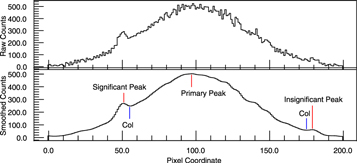
Figure 1. Illustration of peak finding and culling peaks within a footprint. Insignificant peaks within the footprint of a brighter peak are ignored in further processing. Note that this 1D illustration is representative of the full 2D path that may be followed from one peak to the next.
Download figure:
Standard image High-resolution imageSometimes, it is useful to know if a source has a near neighbor that may be affecting the photometry. Three flag bits are used to identify such possible situations. Peaks that are not the brightest peak within a single footprint have the flag bit PM_SOURCE_MODE2_HAS_BRIGHTER_NEIGHBOR set. This is a fairly common situation. We also define the following ratio to compare the flux of the bright source to the flux of a neighbor scaled by intervening area:  where
where  is the flux of the brightest neighbor in the footprint,
  is the flux of the source of interest, and r is the separation between the two sources. If
  , the flag bit PM_SOURCE_MODE2_HAS_BRIGHT_NEIGHBOR_1 is set. If
  , the flag bit PM_SOURCE_MODE2_HAS_BRIGHT_NEIGHBOR_10 is set.
4.4.3. Centroid and Higher-order Moments
Once a collection of peaks has been identified, a number of basic properties of the sources related to the first, second, and higher moments are measured. These moments can be used for a crude classification of the sources. As discussed below, the second moments are used to select candidate stellar sources to be used in modeling the PSF and to identify "cosmic rays" and extended sources. The radial moment is used in the measurement of the Kron magnitudes (Kron 1980). The higher-order moments are provided primarily for image quality diagnostics.
In order to measure the moments, it is necessary to define an appropriate aperture in which the moments are measured. We also apply a "window function," down-weighting the pixels by a Gaussian, centered on the object, with size  chosen to be large compared to the PSF size,
  . This window function reduces the noise of the measurement of the moments by suppressing the noisy pixels at high radial distance as well as by reducing the contaminating effects of neighboring stars. The choice of
  and the aperture is an iterative process: for a given value of
  , the PSF stars will have a measured value of the PSF size,
  which is different from the true value due to the effect of the window function. The measured value of the PSF size will be biased high or low depending on both the signal-to-noise of the source and the size of the window function compared to the true PSF size.
These effects are illustrated in Figure 2 using simulated data. An image was generated with a PSF model matching the radial profile of the PS1 PSF model with  corresponding to an FWHM of 14. For bright stars, as the window function
  is increased, the measured FWHM rises from an initially underestimated value to meet the truth value. For faint stars, the measured value of the FWHM is initially underestimated as well. However, as the value of
  increases, the measured FWHM for faint stars rises and then overshoots the truth value, while the scatter increases. Thus, for large values of
  , the result is both a poorly estimated FWHM for the image and a trend with the S/N of the star. We attempt to minimize the scatter and trends with instrumental magnitude at the cost of overall bias.
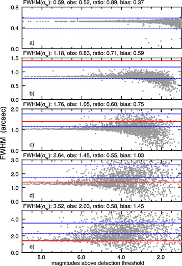
Figure 2. Example of the biases encountered when measuring the second moments. A simulated image was generated using the PS1 PSF profile. Panels (a)–(e) correspond to a different value of  , corresponding to the window FWHM values as marked. The solid red line is the true FWHM of the PSF used to generate the stars (14 in all cases). The blue solid line is the FWHM of the window function. The gray dots are the FWHM derived from the measured second moments for stars in the image. The median of this distribution (mag
  ) is listed as "obs." The ratio of the median FWHM to the FWHM of the window function is listed as "ratio," while the ratio of the median FWHM to the true stellar FWHM is listed as "bias." The dotted blue line is the target (65% of the window function). In this example, we would choose
  between 05 and 08 (FWHM between 264 and 352), so the dotted blue line would match the bright end of the gray dots. See discussion in the text for the choice of target window.
Download figure:
Standard image High-resolution imageIn a real image, we do not know the true value of the PSF size. If we simply choose a very large window function and rely on bright stars, our estimate of the PSF size will be quite noisy. Compounding this problem are the two additional facts that (1) we do not know which are the real stars (as opposed to bright galaxies or possible image artifacts) and (2) the brighter stars are themselves subject to additional biases due to saturation and other nonlinear effects (c.f., "the Brighter-Fatter" effect; Antilogus et al. 2014; Gruen et al. 2015). To make a robust choice for  , we choose a value such that the measured value of
  is 65% of
  . The resulting second-moment values are biased somewhat low (∼75% of the truth value for the PS1 PSF profile) but are relatively unbiased as a function of brightness.
To choose the value of  , we try a sequence of values spanning a range guaranteed to contain any reasonable seeing values. The values are specified in the psphot recipe as PSF.SIGMA.VALUES and have the following values for PS1 PV3: (1, 2, 3, 4.5, 6, 9, 12, 18) pixels ∼(026, 051, 077, 115, 154, 23, 31, 46). For each of these
  values, we then select candidate PSF stars based on the distribution of the measured
  in the two principal directions:
  and
and  (see Section 4.5.2, below). For each test value of
  , we determine the ratio
  , i.e., the ratio of the window size to the observed PSF size. We interpolate to find a value of
  for which
  is expected to be 0.65. We use an aperture with a radius of
  to select the pixels for the measurement of the moments.
Once  has been determined, moments are measured as defined below:

where fi
is the flux in a pixel; si
is the local sky value for that pixel; wi
is the value of the window function for the pixel;  is the window-weighted sum of the source flux, used to renormalize the moments; and ri
is the radius of a pixel,
is the window-weighted sum of the source flux, used to renormalize the moments; and ri
is the radius of a pixel,  . The sums are performed over all (unmasked) pixels in the aperture. For the centroid calculation (
 ), the peak coordinate (see Section 4.4.1) is used to define the aperture and the window function; for higher-order moments, the centroid is used to center the window function.
The motivation for measuring these higher-order moments was to select exposures with image quality problems. For example, trefoil caused by errors in the collimation and alignment can in principle be detected with the third-order moments. In our experience, these statistics can be used to select some images with such problems, but we have not been able to use these values to exclude poor images from the data processing. If we were to reject images based on these moments, we would reject too many images with image quality issues that are not so poor as to preclude a useful analysis. A future machine-learning-based analysis starting with these moments might potentially provide a better rejection statistic, but such work is beyond the scope of this article.
For sources with peak flux above the saturation limit, the moments are generally poorly measured if the aperture defined by  is used. For these sources, the quality of the measurement is compromised by the saturation. However, it is still useful to estimate the first and second moments of the source in order to allow a crude measurement of the brightness from the wings of the source. In this case, a larger aperture, three times the standard aperture, is used to make a crude estimate. For such sources, the flag bit PM_SOURCE_MODE_BIG_RADIUS is set, and the source is ignored in all analyses below except for the analysis applied to very bright stars (Section 4.6.1).
If the measured centroid coordinates ( ) differ from the peak coordinates by a large amount (1.5
 ), then the peak is identified as being of poor quality and is skipped in further analyses; the flag bit PM_SOURCE_MOMENTS_FAILURE is set for such sources. In such a case, it is likely that the "peak" was identified in a region of flat flux distribution or many saturated or edge pixels. During the analysis of the moments, the background ("sky") model is also examined for the location of each source. The value of the background and the variance of the background are recorded for each source. In some cases, the sky model or the variance is not well defined at the location of a specific sources (e.g., due to an extrapolation failure). In these cases, the flag bits PM_SOURCE_SKY_FAILURE or PM_SOURCE_SKYVAR_FAILURE are set as appropriate, and the measurement of the moments is skipped.
In addition to the moments above, the first and half-radial moments, Mr and Mh as defined below, are calculated:
Note that the window function is not applied in the calculation of these moments.
With the first radial moment, we can calculate a preliminary Kron radius and magnitude. Kron magnitudes are provided as an option for galaxy photometry. In addition, the comparison of Kron and PSF magnitudes is useful as a star–galaxy separator. The Kron radius (Kron 1980) is defined the be 2.5× the first radial moment. The Kron flux is the sum of (sky-subtracted) pixel fluxes within the Kron radius. We also calculate the flux in two related annular apertures: the Kron inner flux is the sum of pixel values for the annulus  , while the Kron outer flux is the sum of pixel values for
  . The first radial moment is limited at the low and high ends by
  , where
  is the first radial moment of the PSF stars, or
  if that cannot be determined.
  is set to the size of the moment's aperture,
  . These Kron measurements are performed for all sources with a valid set of moments. At this stage, the measurement of the Kron parameters are preliminary as the aperture has been chosen as a fixed size relative to the size of the PSF. At a later stage, higher-quality Kron parameters appropriate to galaxies are measured with more care paid to the exact aperture used (Section 4.6.4).
4.5. PSF Determination
4.5.1. PSF Model versus Source Model
The PSF of an image describes the shape of all unresolved sources in the image. In a typical wide-field image, the shape of unresolved sources varies as a function of position in the image. The full PSF thus needs to include a model with parameters that vary across the image.
The PSF used by psphot consists of an analytical function combined with a pixelized representation of the residual differences between the analytical model and the true PSF. Both the shape parameters of the analytical model and the pixelized residual differences are allowed to vary in two dimensions across the images.
Within psphot, several analytical models may be used to describe the smooth portion of the PSF, but all share a few common characteristics. As an example, a simple model consists of a 2D elliptical Gaussian:


Here, the model parameters consist of the centroid coordinates ( ), the elliptical shape parameters (
 ), the model normalization (Io
), and the local value of the background (S).
), the model normalization (Io
), and the local value of the background (S).
A specific source will have a particular set of values for the model parameters, some of which depend on the PSF model and the position of the source in the image, while the rest are unique to the individual source. For the case of the elliptical Gaussian model, the PSF parameters would be the shape terms ( ) while the independent parameters would be the centroid, normalization and local sky values (
 ), though as noted below (Section 4.6.6), in practice we do not allow the sky to be fitted independently as we subtract the background model. Thus, the shape parameters are each a function of the source centroid coordinates:


psphot represents the variation in the PSF parameters as a function of position in the image in two possible ways, specified by the configuration. The first option is to use a 2D polynomial that is fitted to the measured parameter values across the image. The second option is to use a grid of values that are measured for sources within a subregion of the image. In the latter case, the value at a specific coordinate in the image is determined via bilinear interpolation between the nearest grid points. The order of the polynomial or the sampling size of the grid is dynamically determined depending on the number of available of PSF stars. In the case of the PV3 analysis, the grid of values was used, with a maximum of 6 × 6 samples per GPC1 chip image (grid cells of size ∼34). For the earlier PV2 analysis, the maximum grid sampling was 3 × 3 per GPC1 chip image (grid cells of size ∼69). For the PV1 analysis, the polynomial representation was used, with up to third-order terms. The higher order representation was used for PV3 in order to follow some of the observed PSF variations in the images.
Figure 3 illustrates the 2D variations in the PSF shapes seen in PS1 data. This figure shows the FWHM and e1 and e2 polarizations of the stars as a function of position in four exposures. For images with good image quality, variations of the PSF shape due to the optical aberrations can be seen. The optical aberrations vary as the active collimation and alignment are adjusted and as the focus changes. These aberrations are coupled to the piston of the chips, which have been adjusted to crudely follow the focal surface (Chambers et al. 2016). During regular operations, images with large PSFs are usually caused by the atmosphere (seeing) or by telescope tracking errors, both of which result in common shapes across the field of the camera. In the figure, the top panel shows the circularization of the PSF due to the atmosphere washing out the lower-level variations caused by the optics.
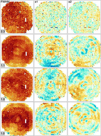
Figure 3. Examples of 2D PSF variations. Each row represents an exposure. The leftmost column shows the distribution of FWHM across the camera; the median value in arcseconds is given in the inset. The middle column gives the e1 polarization measured from second moments (see Section 6.3), while the right column gives the e2 polarization.
Download figure:
Standard image High-resolution imageSeveral analytical functions that are likely candidates to describe the smooth portion of the PSF are available in psphot:
- 1.Gaussian :

- 2.Pseudo-Gaussian :
[PGAUSS]
- 3.Variable Power Law :
[RGAUSS],
- 4.Steep Power Law :
[QGAUSS]
- 5.PS1 Power Law :
[PS1_V1]


The Pseudo-Gaussian is a Taylor expansion of the Gaussian and is used by Dophot (Schechter et al. 1993). The latter profiles are similar to the Moffat profile form (Moffat 1969; Buonanno et al. 1983), with small differences. For these PSF models, the functions are evaluated at the pixel center. Unlike some galaxy model representations (see Section 5.3 ), the first derivatives of these functions approach zero as the radius approaches zero, so subpixel integration is not necessary. A user may choose to try more than one analytical function for a given image. As discussed below (Section 4.5.3), psphot can automatically choose the best model based on the quality of the PSF fits.
For the PS1 GPC1 analysis, we used the PS1_V1 model, which we found by experimentation to match well to the observed profiles generated by PS1. Figure 4 shows example radial profiles for moderately bright stars in fairly good (09) and poor (22) seeing. Using a fixed power-law exponent results in somewhat faster profile fitting compared to the variable power-law exponent model.
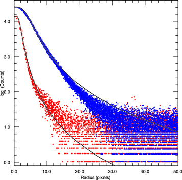
Figure 4. Radial profiles of stellar images from PS1. These two profiles illustrate the radial trend of the PS1 PSFs for a star with FWHM 09 (red) and 22 (blue). The red and blue points are individual pixel values. The black line shows the PSF model with radial trend of the form  . The models use a 1D average of the 2D analytical portion of the PSF models fitted to these specific stars in their standard analysis.
Download figure:
Standard image High-resolution imageThe analytical models in psphot are written with a high degree of code abstraction, making it relatively easy to add different analytical models to the software. The same portion of code used to describe the analytical portion of the PSF sources is also used for galaxy models.
Once the smooth component of the PSF has been fitted with an analytical model, a pixel representation of the residuals is generated. This representation is constructed as an image of the expected residuals for any position in the image. The value of each pixel in the image model is determined from 2D fits to the measured residuals of the PSF stars.
The residual model is calculated using the residuals for all PSF stars. The residuals (and their errors) for each star are renormalized by the flux of the star to put them on a consistent flux scale. For each PSF star, all pixels within a user-specified radius (PSF.RESIDUALS.RADIUS=9) are selected for the measurement. For a given pixel in the model, the value is calculated from the four closest pixels in the PSF stars via bilinear interpolation. Pixels may be used in this analysis if their S/N exceeds a user-defined limit. For the PV3 3π analysis, we allowed all pixels within the user-specified radius, not limiting on the basis of the S/N.
Pixels for a given star that are more than a number of sigmas (PSF.RESIDUALS.NSIGMA=3.0) deviant from the median value of the pixels from all stars are rejected.
If no spatial variation is allowed, the mean or median value is calculated for the model pixel based on the user-specified mean statistic (PSF.RESIDUALS.STATISTIC=ROBUST_MEDIAN).
If spatial variation is requested, then the pixel values are fitted to a linear model:
where ![$R[({x}_{\mathrm{mod}},{y}_{\mathrm{mod}})][({x}_{\mathrm{ccd}},{y}_{\mathrm{ccd}})]$](https://content.cld.iop.org/journals/0067-0049/251/1/5/revision3/apjsabb82cieqn77.gif) is the value of the residual for model pixel
is the value of the residual for model pixel  for a star with centroid at image pixel
  . The parameters
  are the elements of the 2D linear fit for each pixel
  in the model.
4.5.2. Candidate PSF Source Selection
The first stage of determining the PSF model for an image is to identify a collection of sources in the image which are likely to be unresolved (i.e., stars). psphot uses the source sizes as estimated from the second moments to make the initial guess at a collection of unresolved sources. At this point, the program has measured the second-order moments for all sources identified by their peaks, as well as an approximate S/N, above the bright threshold. All sources with an S/N greater than a user-defined parameter (PSF_SN_LIM = 20.0 for PS1 PV3) are selected by psphot, though sources that have more than a certain number of saturated pixels are excluded at this stage. The program then examines the 2D plane of  in search of a concentrated clump of sources (see Figure 5). To do this, it constructs an artificial image with pixels representing the value of
  , using
  as the size of a pixel in this artificial image. The binned
  plane is then examined to find a significant peak. Unless the image is extremely sparse, such a peak will be well defined and should represent the sources which are all very similar in shape. Other sources in the image will tend to land in very different locations, failing to produce a single peak. To avoid detecting a peak from the unresolved cosmic rays, sources that have second moments very close to 0 are ignored. For these sources, the flag bit PM_SOURCE_MODE_DEFECT is set.
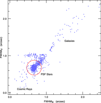
Figure 5. Illustration of PSF star selection using the second moments. Each point represents the second moments in the  and
and  directions for sources measured in one chip (XY32) from a particular PS 1 exposure (o6065g0428o). The dominant clump is located in this diagram to identify the stars. Galaxies tend to have a range of sizes and thus spread out above the stars. Cosmic rays also have a range of sizes, with one dimension smaller than the PSF. The red circle represents the PSF star candidates.
Download figure:
Standard image High-resolution imageOnce a peak has been detected in this plane, the centroid and second moments of this peak are measured. All sources that land within 2 pixels of this centroid are selected as candidate PSF sources in the image.
When the second moments are measured, psphot also counts the number of saturated pixels within the analysis aperture. If more than a single saturated pixel is found, and if the second moments of that object are more than one standard deviation larger than the clump identified above, this source is identified as a highly saturated star and marked with the flag bit PM_SOURCE_MODE_SATSTAR. Sources that have more than a single saturated pixel, but for which the second moments do not exceed the above limits, are marked as likely saturated regions (e.g., bleed trails). These sources are skipped in most additional analyses and are marked with the flag bit PM_SOURCE_MODE_SATURATED.
4.5.3. Candidate PSF Source Model Fits
All candidate PSF sources are then fitted with the selected source model, allowing all of the parameters (PSF and independent) to vary in the fit. The software uses the Levenberg–Marquardt minimization technique (e.g., Press et al. 1992; Madsen et al. 2004) for the nonlinear fitting. Nonlinear fitting can be very computationally intensive, particularly if the starting parameters are far from the minimization values. The first and second moments are used to make a good guess for the centroid and shape parameters for the PSF models. Any sources that fail to converge in the fit are flagged as invalid.
To generate the initial guess, the second moments are converted to the equivalent sigma values for a 2D elliptical Gaussian contour using the following transformations inspired by Bertin & Arnouts (1996) and Stobie (1980). First, we calculate the sigma values in the major ( ) and minor (
 ) axis directions, along with the position angle θ from the moments using


where the function arctan2 (y, x) returns the arctangent in the proper quadrant (e.g,. as implemented by the atan2(y,x) function in C) and the intermediate values g1, g2, g3 are given by


Because the moments may be noisy, the calculated value of  can be numerically invalid if
  , a situation that is especially likely for highly elongated sources. We avoid this situation by limiting the axial ratio to a maximum of 20 (setting
  to
to  if the expected axial ratio would be greater than this limit). The selected value of 20 is somewhat ad hoc, chosen based on failures in real images. A more careful examination of the trade-off space would be worthwhile in the future.With
  ,
,  , and θ in hand, we can now transform these values to the parameters of our fits,
  ,
,  , and
, and  (Equation 20 above). This transformation can be determined by rotating the 2D Gaussian equation, yielding


In fact, because the calculated second moments have been measured with a window function applied (see discussion in Section 4.4.3), we instead use the measured value of Mr
(Equation 18), the first radial moment as the major-axis size for the Gaussian ( ), retaining the position angle and axial ratio from the calculation above. We use these guess parameters for all versions of the PSF analytical models, despite the fact that for the versions which are not approximations of Gaussians these guess values will be systematically incorrect. It would be worthwhile in the future to tweak the guesses for the different model version to speed up the convergence.
For the resulting collection of source model parameters, the PSF-dependent parameters of the models are all fitted as a function of position using either the 2D polynomial or the gridded representation described above. The maximum order of these fits depends on the number of PSF sources (see Table 6). The fitting process for these polynomials is iterative and rejects the 3σ outliers in each of three passes. This fitting technique results in a robust measurement of the variation of the PSF model parameters as a function of position without being excessively biased by individual sources that are not well described by the PSF model (e.g., galaxies that snuck into the sample). Sources whose model parameters are rejected by this iterative fitting technique are also marked as invalid PSF sources and ignored in the later PSF model fitting stages. Sources that are actually used to define the PSF model for a given image have the flag bit PM_SOURCE_MODE_PSFSTAR set.
Table 6. Minimum Number of Stars Required for a Given Order of the PSF 2D Variations, or for the Given Number of Grid Cells
| Minimum | Order | Number of | Cell Size |
|---|---|---|---|
| # of Stars | Grid Cells | (arcmin) | |
| 16 | 1 | 4 | 10.3 |
| 54 | 2 | 9 | 6.9 |
| 128 | 3 | 16 | 5.1 |
| 300 | 4 | 25 | 4.1 |
| 576 | 5 | 36 | 3.4 |
Download table as: ASCIITypeset image
The order of the fit or number of grid samples is modified if the number of stars available for the fit is insufficient to justify the highest value. Regardless of the requested order, if the number of stars is below the following limits, the order is limited as shown in Table 6. Note that the number of grid cells in one dimension is one greater than the equivalent polynomial order.
All of the PSF candidate sources are then refitted using the PSF model to specify the PSF-dependent model parameter values for each source. For example, in the case of the elliptical Gaussian model, the shape parameters ( ) for each source are set by the coordinates of the source centroid and fixed (not allowed to vary) in the fitting procedure. The resulting fitted models are then used to determine a metric that tests the quality of the PSF model for this particular image.
psphot allows a collection of PSF model functions to be tried on all PSF candidate sources. The number of models to be tested is specified by the configuration keyword PSF_MODEL_N. The configuration variables PSF_MODEL_0, PSF_MODEL_1, through PSF_MODEL_N---1 specify the names of the models that should be tested. The metric used by psphot to assess the PSF model is the scatter in the differences between the aperture and fit magnitudes for the PSF sources. This difference is a critical parameter for any PSF modeling software as it is a measurement of how well the PSF model captures the flux of the star. Aperture photometry is measured for a circular aperture with a radius of PSF_APERTURE_SCALE (4.5 for PV3) times  (Section 4.4.3). The average aperture correction (
 ) is measured and, if multiple PSF model types are selected, the PSF model with the minimum clipped scatter in this statistic is chosen for the image. For the PV3 analysis, however, only the PS1_V1 model function was used.
An approximate aperture correction is measured at this stage, with a more detailed correction measured after all source analysis is performed (see Section 4.8). Sources for which the aperture magnitude is measured have the flag bit PM_SOURCE_MODE_AP_MAGS set. These aperture magnitudes are stored in the DVO field Measure.Map and exported to the PSPS as a flux in Janskies in the field Detection.apFlux. The radius (in arcseconds) of the aperture used for each exposure is reported in PSPS as Detection.apRadius, while the unmasked fraction of the aperture is reported in PSPS as Detection.apFillF.
As noted above (Section 4.3), we do not attempt to replace or interpolate masked pixel values. Aperture photometry measurements of objects that include masked pixels are thus inaccurate. For a stellar object, the amount of error is a function of how close the masked pixels are to the core of the PSF. To provide guidance, when the PSF and aperture photometry for a source are measured, two additional quantities that are useful to assess the impact of masking are measured. First, the mask image is examined and the number of unmasked pixels is summed, weighted by the normalized PSF model. The resulting quantity, PSF_QF, has a value between 0.0 (totally masked) and 1.0 (totally unmasked). Elsewhere in the IPP system, we use this value to filter out detections that are unreliable due to the masking. For a generous cut, leaning toward completeness at the cost of some lower-quality measurements, PSF_QF
 is used in some contexts; in other cases, we require PSF_QF
 to ensure a high-quality measurement (see, for example, the calculation of average photometry in Magnier et al. 2020b). The second quantity is related to the first: PSF_QF_PERFECT uses all mask values to assess the quality factor, while PSF_QF uses only the "bad" mask bit values (see Section 4.3).
Several flag bits are raised based on statistics that are similar to the PSF_QF measurement. First, psphot calculates the normalized, PSF-weighted fraction of pixels that are masked due to one of the following four causes: a diffraction spike (SPIKE), the core of a saturated star (CORE), burntool-subtracted region (BURNTOOL), or a pixel for which, due to interpolation or convolution, a significant fraction of the pixel flux comes from a masked pixel. These masking conditions are all treated as "suspect" by psphot, which means they are included in the analysis of the source pixels. However, because they may potentially affect the photometry (or astrometry), it is useful to note a source that has a nontrivial fraction of these poor mask pixels. If the normalized PSF-weighted fraction of pixels masked due to any of these four conditions exceeds 25%, then one of the following bits is raised for the corresponding condition: PM_SOURCE_MODE2_ON_SPIKE, PM_SOURCE_MODE2_ON_STARCORE, PM_SOURCE_MODE2_ON_BURNTOOL, PM_SOURCE_MODE2_ON_CONVPOOR. In addition, the following flag bits may also be raised if the central pixel of a source lands on a pixel masked for a diffraction spike (PM_SOURCE_MODE_ON_SPIKE), an optical ghost (PM_SOURCE_MODE_ON_GHOST), or off the active pixels of the CCD (PM_SOURCE_MODE_OFF_CHIP).
4.6. Bright-source Analysis
Once a PSF model has been determined, the brighter sources in the image may be analyzed in detail. The goals in this stage are (1) to determine the fluxes and positions of the bright stellar sources with high precision appropriate to their high S/N and (2) to characterize the bright source flux profiles sufficiently well that they may be subtracted from the image to allow for the clean detection of the fainter sources. Note that as the analysis proceeds, there are several stages in which the 2D flux models for all sources are subtracted from the image, and individual sources are replaced in the image for a particular analysis step and then removed again. The flux limit for this analysis stage is user defined as an S/N value. In the PV3 analysis of the 3π Survey data, this limit was set to an S/N of 20.0.
In order to allow for multiple threads to process a single image, the pixels in an image are divided into a grid of superpixels (note that these superpixels are not the same as those used for either the background model or the PSF parameter variations). The superpixels are assigned to one of four groups so that each superpixel in a group is well separated from the other superpixels of that group. The analysis of the image proceeds in four steps, one for each of these groups. Each of the superpixels in the first group is assigned to a single thread until all threads are assigned. A single thread is responsible for the analysis of sources that land within their current superpixel, as determined by the centroid coordinates. Because the superpixels in a given thread group are not contiguous by construction, sources near the edge of a superpixel can be analyzed by considering the nearby pixels from a neighboring superpixel (guaranteed not to be in the current thread group).
As the threads complete their analysis, they are assigned the next unfinished superpixel in the active group. When all superpixels in one group have been processed, then the superpixels in the next group can start. This strategy allows the threading to process sources that may be extended without the danger that two threads are actively touching the same pixels. For the PV3 analysis, four threads were used for most processing tasks.
4.6.1. Very Bright Stars
The standard psphot PSF modeling code fails to fit the wings of highly saturated stars, especially if the core of the star is too contaminated by saturated pixels. For stars with more than a single saturated pixel, we model the radial profile of the logarithmic instrumental flux in logarithmically spaced radial bins. For each radial bin, we determine the median of the log flux. This median profile is then interpolated to generate the full radial flux distribution. Note that in the case of very saturated stars, pixels in the central regions are largely masked, because they are saturated. Thus, in these cases, the PSF-weighted masked fraction (see Section 4.5.3) is generally quite low or 0.0. Sources for which this radial profile is subtracted have the flag bit PM_SOURCE_MODE2_SATSTAR_PROFILE set.
4.6.2. Fast Ensemble PSF Fitting
Before the detailed analysis of the sources is performed, it is convenient to subtract off all of the sources, at least as well as possible at this stage. We make the assumption that all sources are PSF like. If the centroid of the source has been determined, we use this value for its position; otherwise, we use the interpolated position of the peak. A single linear fit is used to simultaneously measure all source fluxes. Because the local sky has been subtracted, this measurement assumes the local sky is zero. We can write a single  equation for this image:
where  is image flux for each pixel,
 ![$P[{x}_{0},{y}_{0}]$](https://content.cld.iop.org/journals/0067-0049/251/1/5/revision3/apjsabb82cieqn107.gif) is the PSF model realized at the position of source i, and Ai
is the normalization for the source.
is the PSF model realized at the position of source i, and Ai
is the normalization for the source.
Minimizing this equation with respect to each of the Ai values results in a matrix equation:

where  is the vector of Ai
values, the elements of
is the vector of Ai
values, the elements of  consist of the dot products of the unit-flux PSF for source i and source j, and
  is the dot product of the unit-flux PSF for source j with the pixels corresponding to source j. The dot products are calculated only using pixels within the source apertures. Because most sources have no overlap with most other sources, this matrix equation results in a very sparse, mostly diagonal square matrix. The dimension is the number of sources, likely to be 1000 s or 10,000 s. Direct inversion of the matrix would be computationally very slow. However, an iterative solution quickly yields a result with sufficient accuracy. In the iterative solution, a guess at the solution
  is made assuming
  is purely diagonal; the guess is multiplied by
  , and the result is compared with the observed vector
  . The difference is used to modify the initial guess. This process is repeated several times to achieve convergence. Convergence is quick (a few iterations) because of the highly diagonal matrix with small off-diagonal terms: the dot product of source i and source j is 1, where i = j and much less than 1 where
  .
.
Once a solution set for Ai is found, all of the sources are subtracted from the image by applying these values to the unit-flux PSF. Sources for which a PSF model has been fitted (whether or not this is retained as the best model in the end) has the flag field PM_SOURCE_MODE_PSFMODEL set. All sources that are included in the ensemble linear fit have the flag bit PM_SOURCE_MODE_LINEAR_FIT set, including those for which the model is not the PSF.
4.6.3. Radial Profile Wings
We attempt to measure the radial profile of sources in order to find the radius at which the flux of the source matches the sky. In this analysis, a series of up to 25 radial bins with power-law spacing are defined and the flux of the source in each annulus is measured. The "sky radius" is defined to be the radius at which the (robust median) flux in the annulus is within 1σ of the local sky level. If this limit is not reached before the slope of the flux from one annulus to the next is less than a user-defined limit, then the annulus at which the slope reaches this limit is used to define the sky radius. These values are saved in the output FITS catalog files but not sent to the PSPS. The sky radius value is used below in the calculation of the Kron magnitude.
4.6.4. Kron Magnitudes
Preliminary Kron radius and flux values (Kron 1980) are calculated soon after sources are detected (Section 4.4.3). However, these preliminary values are not accurate due to the window functions applied. After sources have been characterized and the PSF model is well determined, the Kron parameters are recalculated more carefully. In this version of the calculation, following the algorithm described by Bertin & Arnouts (1996), the image is first smoothed by a Gaussian kernel with  pixels, corresponding to an FWHM of 10 in the PS1 stack images. Next, the Kron radius is determined in an iterative process: the first radial moment is measured using the pixels in an aperture 6× the first radial moment from the previous iteration. On the first iteration, the sky radius is used in place of the first radial moment. By default, two iterations are performed. The Kron radius is defined to be 2.5× the first radial moment. The Kron flux is the sum of pixel fluxes within the Kron radius. We also calculate the flux in two related annular apertures: the Kron inner flux is the sum of pixel values for the annulus
  , while the Kron outer flux is the sum of pixel values for
  .
.
Two details in the calculation above should be noted. First, for faint sources, noise in the measurement of the first radial moment may result in an excessively small aperture for the successive calculations. The window used for the calculations is constrained to be at least the size of the aperture based on the PSF stars (Section 4.4.3). At the other extreme, noise may make the radius grow excessively, resulting in an unrealistically low effective surface brightness. The aperture is constrained to be less than a maximum value defined such that the minimum surface brightness is 1/2× the effective surface brightness of a point source detected at the 5σ limit.
Second, the measurement of the first radial moment includes a filter to reduce contamination from outlier pixels. Pairs of pixels on opposites sides of the central pixel are considered together. The geometric mean of the two fluxes is used to replace the flux values. If the source has 180° symmetry, this operation has no impact. However, if one of the two pixels is unusually high, the value will be suppressed by the matched pixel on the other side. This trick has the effect of reducing the impact of pixels that include flux from near neighbors. We found it necessary to apply this filter because, although the source models have been subtracted, at this point in the analysis, only PSF models have been used. Thus, extended objects (galaxies) can leave behind significant amounts of flux to contaminate the neighbors.
4.6.5. Source-size Assessment
After the PSF model has been fitted to all sources and the Kron flux has been measured for all sources, psphot uses these two measurements, along with some additional pixel-level analysis, for classification based on source size. Sources identified as extended will be fitted with a galaxy model (or possibly another type of extended source model in special cases). If the source is small compared to a PSF, it is considered to be a cosmic ray and masked.
Extended sources are identified as those for which the Kron magnitude is significantly brighter than the PSF magnitude when compared to a PSF star. The value  , the difference between the PSF and Kron magnitudes, is calculated for each source. The median of
  is calculated for the PSF stars. This median is subtracted from
  for each star. The result is divided by the quadrature error of the PSF and Kron magnitudes and called extNsigma. If extNsigma is larger than the configuration value PSPHOT.EXT.NSIGMA.LIMIT (3.0 for PV3), the source is considered to be extended, and the flag bit PM_SOURCE_MODE_EXT_LIMIT is set for the source.
We decided to use the  metric for this assessment after we tested several possible star–galaxy separation statistics. We found that the Kron PSF comparison was more reliable than second-moment and first-radial-moment based measurements. In addition, because we needed a statistic that could be calculated relatively quickly on every detected source, we rejected using a galaxy model fit for the star–galaxy separator.
Cosmic rays are identified by a combination of the Kron magnitude and the second-moment width of the source in the minor axis direction. The second moment in the minor axis direction is calculated from  as follows:
If  pixels2 and the S/N of the flux measured in the moments analysis
  , then the source is identified as a cosmic ray and the associated pixels are masked. These values are tuned empirically for the PV3 analysis based on cosmic rays identified in the GPC1 images. Sources that are determined to be a cosmic ray in this manner have the flag bit PM_SOURCE_MODE_DEFECT set.
The pixels of any suspected cosmic ray identified above are examined in additional detail to make a final judgment. The Laplacian edge detection algorithm based on van Dokkum (2001) is used to check for sharp edges in the flux distribution. If the sharpness exceeds a defined limit, then the pixels are masked and the flag bit PM_SOURCE_MODE_CR_LIMIT is set for the source.
4.6.6. Full PSF Model Fitting
At this point, we have a PSF model for the image, we have an assessment of the size (PSF like, extended, or cosmic ray) for each object, and we have fitted the PSF model for the normalization to each source (Section 4.6.2). However, the positions for the sources have been fixed to the position determined from the peak-detection stage (Section 4.4.1) or the centroid from the analysis of the moments (Section 4.4.3). A better position, and thus a better normalization, can be determined by simultaneously fitting for all three parameters. We therefore go through the image and refit the PSF model to each source one at a time, with all other sources subtracted based on the earlier fit.
This refitting analysis is performed for all of the sources with S/N greater than a user-defined limit. In the PV3 analysis of the 3π Survey data, this limit was set to an S/N of 20.0 for the chip and stack analysis stages. In these fits, the dependent parameters are fixed by the PSF model and only the three independent source model parameters (position in X and Y and flux normalization) are allowed to vary in the fit. Note that we do not allow the local sky to be fitted as a free parameter. As we have subtracted a model for the background, allowing the sky to be fitted again at this stage is redundant. In fact, in our testing, we found that allowing the sky background value to float resulted in a higher scatter for the flux normalizations. For the nonlinear fitting, psphot again uses the Levenberg–Marquardt technique. The sources are fitted in their S/N order, starting with the brightest and working down to the user-specified limit, with the other sources subtracted as discussed above. All sources for which a nonlinear PSF model has been attempted have the flag bit PM_SOURCE_MODE_FITTED set, regardless of the quality of that fit.
Because the PSF model describes the variation of the PSF across the image, the parameters used to fit a specific object are drawn from the model at the position corresponding to the object centroid. Occasionally, a PSF model for an image may not be well determined in all regions of the image. For example, not enough bright stars were available across the full range of the image to model the PSF and the resulting fitted parameters yield nonsensical solutions in areas where detected (fainter) sources are found. In such cases, the PSF fitting is skipped and the flag bit PM_SOURCE_MODE_BADPSF is set.
For the PSF model fitting, only pixels within a circular aperture scaled based on the seeing are used. The radius of the circular aperture is set to be a fixed multiple (PSF_FIT_RADIUS_SCALE) of  , the width of the Gaussian window function determined based on the analysis of the second moments (see Section 4.4.3). For the PV3 3π analysis, the PSF fit window radius is
  .
.
After the PSF model is fitted to each object, psphot makes an assessment of the quality of the PSF fits. First, it checks that the nonlinear fitting process has converged with a valid fit. The fit for an object can fail if there are too few valid pixels, due to masking or proximity to an edge, or if the parameters are driven to extreme values which are not permitted. In addition, it is possible for the peak-finding algorithm to identify peaks in locations that are not actually a normal peak. Some of these cases are in the edges of saturated, bleeding columns from bright stars, in the nearly flat halos of very bright stars, and so on. In these cases, a local peak exists, with a lower nearby sky region. However, the fitted PSF model cannot converge on the peak because it is very poorly defined (perhaps only existing in the smoothed image). In these cases, psphot flags the object with the bad bit PM_SOURCE_MODE_FAIL. It is also possible in this type of case for the fit to result in a very low or negative value for the flux normalization parameter. Sources for which the peak is less than 0.02 are also marked as failing the nonlinear PSF fit (PM_SOURCE_MODE_FAIL).
Poor fits are also identified by the S/Ne and the  value of the resulting fit. If a source has a PSF S/N lower than a user-defined cutoff (set to 2.0 for the PV3 analysis of the 3π Survey), the nonlinear PSF fit will be rejected. If the
  per degree of freedom is greater than a user-defined limit (set to 50.0 for the PV3 analysis of the 3π Survey), the nonlinear PSF fit will be rejected. These sources are marked with the flag bit (PM_SOURCE_MODE_POOR).
Sources that pass the above tests are marked as having a valid nonlinear PSF model fit with the flag bit PM_SOURCE_MODE_NONLINEAR_FIT. Among these sources, those for which the peak flux is greater than the saturation limit (see Section 4.3) are marked as saturated stars (PM_SOURCE_MODE_SATSTAR). These model fits should be considered with caution, but the fluxes and positions may have some validity.
As the sources are fitted to the PSF model, those that survive the exclusion stage are subtracted from the image. The subtraction process modifies the image pixels (removing the fitted flux) but does not modify the mask or the variance images. The S/N in the image after subtraction represents the significance of the remaining flux. If the subtractions are sufficiently accurate models of the PSF flux distribution, the remaining flux should be normally distributed about zero with a standard deviation of 1σ. In practice, the cores of bright stars are poorly represented and may have larger residual significance.
4.6.7. Double and Blended Sources
In fields with high stellar density, the nonlinear source fitting can be adversely affected by close neighbors. We implemented two modifications of the nonlinear fitting code to address this issue for different scales to the nearby neighbors. One version addresses the case of nearby sources that are separately detected in the peak-detection stage; the other version of the analysis attempts to fit a pair of PSFs for sources which are apparently extended. Note that for DR1 & DR2, neither of these options were used because they tended to prevent galaxies from being fitted as extended objects; these rules for distinguishing blended stars and galaxies will be revisited in future reanalyses. We outline the strategy below, although it was not used for these data releases.
Sources that are blended with other sources may be fitted together as a set of PSFs. Blended objects are identified by first searching for objects for which the PSF fit windows overlap. For a group of such neighboring objects, a contour is determined in the flux image at 25% of the peak of the brightest source in the group. All objects lying within this contour are treated as blends of this brightest source. If other objects in this group exist, the brightest object not already assigned to a blend is used to define the contour for blends of this next object. All objects in the image are tested as possible blends. A single multisource fit is performed on each group of blended peaks. Sources that are identified as members of a blended group have the flag bit PM_SOURCE_MODE_BLEND set, while those for which a blended PSF fit succeeds have the flag bit PM_SOURCE_MODE_BLEND_FIT set. For sources in groups of blended stars, the resulting fits are evaluated independently. Any that are determined to be valid PSF fits are subtracted from the image and kept for future analysis.
Sources that are judged to be non-PSF-like are confronted with two possible alternative choices: double star or extended source model (see next section). For the double-star model, the assumption is made that there are two neighboring PSF-like sources, but the peaks are not resolved. The initial guess for the two peaks is made by splitting the flux of the single source in half and locating the two starting peaks at ±2 pixels from the original peak along the direction of the semimajor axis of the sources, as measured from the second moments. In order for the two-source model to be accepted, both sources must be judged as a valid PSF source. Otherwise, the double-PSF model is rejected, and the source is fitted with the available non-PSF model or models. Sources for which a double-PSF model is fitted have the flag bit PM_SOURCE_MODE_PAIR set.
4.6.8. Non-PSF Sources
Once every source (above the S/N cutoff) has been confronted with the PSF model, the sources that are thought to be extended (resolved) can now be fit with an appropriate model (e.g., galaxy profile or other likely extended shapes). Again, the fitting stage starts with the brightest sources (as judged by the rough S/N measured from the moments aperture) and working to a user defined S/N limit.
The choice of extended source model or models is set by the user for a given analysis. In the configuration system, the keyword EXT_MODEL is set to the model of interest. All suspected extended sources are fitted with the model, allowing all of the parameters to float. The initial parameter guesses are critical here to achieving convergence on the model fits in a reasonable time. The moments and the pixel flux distribution are used to make the initial parameter guess. Many of the source parameters can be accurately guessed from the first and second moments. The power-law slope can be guessed by measuring the isophotal level at two elliptical radii and comparing the ratio to that expected.
For each type of extended source model (in fact for all source models), a function that examines the fit results and determines if the fit can be considered as a success or a failure is defined. The exact criteria for this decision depend on the details of the model, and so this level of abstraction is needed. For example, in some case, the range of valid values for each of the parameters must be considered in the fit assessment. In other cases, we may choose to use only the parameter errors and the fit chi-square value.
All extended source model fits that are successful are then subtracted from the image as is done for the successful PSF model fits. The background flux is retained, with the result that only the source is subtracted from the image. At this stage, the variance image is not modified.
For the single-exposure (chip) and stack image analysis, these galaxy model fits are only used internally to generate a clean object-subtracted residual image. For the PV3 analysis of the 3π Survey, these model fits were saved in the output catalog files but not loaded to the public database. The QGAUSS extended source model was used for the PV3 analysis (see Section 4.5.1). The convolved galaxy model fits (see Section 5.3) and the forced galaxy model fits (see Section 6.2) provide more reliable and physically motivated galaxy models.
For the difference image analysis, a trailed object model is used for the extended sources; these model fit parameters are passed to the Moving Object Processing System (MOPS; Denneau et al. 2013).
Any source that is fitted with the extended source model has the flag field PM_SOURCE_MODE_EXTMODEL set.
4.7. Faint Source Analysis
After a first pass through the image, in which the brighter sources above a high threshold level have been detected, measured, and subtracted, psphot optionally begins a second pass at the image. Some of the steps described in the previous sections are repeated in this analysis, though with some modifications as discussed below.
The source detection steps described in Section 4.4 are repeated. To start, the sources detected in the previous steps are subtracted from the image, and the variance enhanced by adding the variance predicted by the model to the variance image, doubling the effective variance at the location of previously detected sources. As in Section 4.4.1, the image is smoothed, but in this pass, it is convolved with the PSF determined above, not a placeholder Gaussian. The new peaks are detected on the smoothed image. The peak-detection process again uses the variance image to test the significance of the individual peaks. All peaks with a significance greater than a user-defined minimum threshold are accepted as sources of potential interest. Footprints are again generated as in Section 4.4.2.
Next, moments are measured as in Section 4.4.3. In this pass, however, the size of the window function applied for the measurement of the moments is fixed at the value determined from the bright source analysis. All sources, including those measured in the bright-source analysis (which are readded to the image and their variance reset), are then simultaneously fit for their flux normalizations as in Section 4.6.2. In this step, the "best" model is used for each source, either a PSF model or the unconvolved extended source model determined in Section 4.6.8. For the newly detected sources, the PSF model is used, with the position set by the centroids.
After the flux normalization is calculated, the radial profile is measured (Section 4.6.3) and the moments are used to calculate the preliminary Kron radius and flux (see Section 4.6.4). These are in turn used to assess the source sizes as in Section 4.6.5. However, the nonlinear fitting steps for the PSF model fits (Section 4.6.6), and the extended source model fits (Section 4.6.8) are not performed for these faint sources. These steps are skipped for two reasons: first, the nonlinear fitting steps are costly in terms of computation time and the faint sources usually far outnumber the brighter sources. Second, because these are faint sources, they do not have the S/N to constrain models with many additional parameters. In addition, the positions (for PSF sources) are not much improved using the nonlinear fitting compared with the nonparametric centroid measurement for these faint sources.
The PV3 threshold for the bright source analysis is an S/N of 20. The flag bit PM_SOURCE_MODE2_PASS1_SRC is raised for sources detected in this initial analysis stage. The lower limit cutoff for the faint source analysis in PV3 is an S/N of 5.0.
In the psphotStack version of the code, the five filter images are processed together. In this case, any source that is detected in at least two of the five filters are then also measured on the other filter images in which it was not detected above the S/N limit. The position in the other stack images is fixed based on the pixel coordinates in the images in which the source was detected. Detection in two filters is required in order to avoid excessive forced photometry of spurious detections. There is an interesting class of astronomical objects that are extremely red (e.g., brown dwarfs and high-redshift quasars). Such sources are expected to be detected only in the reddest filter ( ). For the 3π PV3 processing, we therefore also force the photometry in all filters for sources that are only detected in
  . All sources that are forced on one image based on detections in other images have the flag bit PM_SOURCE_MODE2_MATCHED set.
4.8. Aperture Correction and Total Aperture Fluxes
A PSF model will always fail to describe the flux of the stellar sources at some level. For high-precision photometry, we need to be able to correct for the difference between the PSF model fluxes and the total flux of the sources. In the end, all astronomical photometry is in some sense a relative measurement between two images. Whether the goal is calibration of a science image taken at one location to a standard star image at another location, or the goal is simply the repetitive photometry of the same star at the same location in the image, it is always necessary to compare the photometry between two images. If this measurement is to be consistent, then the measurement must represent the flux of the stars in the same way regardless of the conditions under which the images were taken, at least within some range of normal image conditions. So, for example, two images with different image quality, or with different tracking and focus errors, will have different PSF models. To the extent the PSF model is inaccurate, the measured flux of the same source in the two images will be different (even assuming all other atmospheric and instrumental effects have been corrected). The amplitude of the error will by determined by how inconsistently the models represent the actual source flux.
Aperture photometry attempts to avoid these problems but introduces other difficulties. In aperture photometry, if a large-enough aperture is chosen, the amount of flux that is lost will be a small fraction of the total source flux. Even more importantly, as the image conditions change, the amount lost will change by an even smaller fraction, at least for a large aperture. Aperture photometry can then be used to correct the PSF photometry.
The difficulty for aperture photometry is the need to make an accurate measurement of the local background for each source. As the aperture grows, errors in the measurement of the sky flux start to become dominant. If the aperture is too small, then variations in the image quality are dominant. The brighter the source, the smaller the error introduced by the large size of the aperture. However, the number of very bright stars is limited in any image, and of course, the brighter stars are more likely to suffer from nonlinearity or saturation.
In order to thread the needle between these effects, psphot measures the aperture photometry on a modest-sized aperture and then uses the PSF model to extrapolate to a large aperture. When the PSF fluxes are calculated, the aperture flux for the modest-sized aperture is also determined. The aperture is a circular aperture with radius set to a fixed multiple (PSF_APERTURE_SCALE) of  , the width of the Gaussian window function determined based on the analysis of the second moments (see Section 4.4.3). For the PV3 3π analysis, the aperture window radius is
  , while the large reference aperture radius is set to 25 pixels (PSF_REF_RADIUS = 64). These corrected aperture magnitudes are saved in the output catalogs as AP_MAG, the uncorrected aperture magnitudes are saved as AP_MAG_RAW, and the radius used to measure the raw aperture flux is saved as AP_MAG_RADIUS. The corresponding flux and the flux error are saved as AP_FLUX and AP_FLUX_SIG.
With these aperture magnitudes in hand, it is now possible to make an average correction to the PSF magnitudes to bring the PSF and aperture magnitudes to the same system. This correction is measured using the same stars from which the PSF model is measured, as long as the PSF magnitude error for the star is less than 0.03 mag. The correction is calculated using the weighted average of the values  . Because the PSF may vary across the image, the correction is determined as a function of position in the image. Like the PSF model, the 2D variations of the aperture correction may be modeled as a polynomial or via interpolation in a grid. For the 3π PV3 analysis, a grid with a maximum of 6 × 6 samples per GPC1 chip image was used. The reported PSF magnitudes for all objects have this aperture correction applied. Note that an initial aperture correction was measured during the initial steps of the analysis before the PSF model was chosen. However, because the sources in the image were not yet measured and subtracted, that aperture could be contaminated by neighbors. The analysis here is performed one fairly bright star at a time with all other sources subtracted in order to minimize such contamination.
4.9. Completeness and Contamination
At the end of the psphot analysis of the sources in the image, an analysis is performed to test the detection efficiency. A number of fake PSF sources are injected into the image and the peak-detection analysis (Section 4.4.1) is used to determine if these sources would have been recovered. The PSF model fluxes are measured for the source that are detected. For a given image, the detection threshold is predicted based on the median image variance and the seeing. A series of brightness bins straddling the threshold are defined and a number of sources are injected with magnitudes corresponding to each of these bin values. The psphot recipe value EFF.NUM specifies the number of sources in each brightness bin (500 the PV3), and the value @EFF.MAG specifies the bins as magnitudes above and below the threshold. For PV3, the 13 mag offsets were (−2.0, −1.0, −0.5, −0.25, −0.1, −0.05, 0.0, 0.05, 0.1, 0.25, 0.5, 1.0, 2.0), providing fine sampling near the limit, but coarser coverage farther away. Poisson noise appropriate to the photon counts of the injected sources is included in the image. Injected sources are uniformly distributed across the image in X and Y pixel coordinates without any consideration of the masked regions. This last point means the recovered fraction in the bright bins can be used to test the masking fraction.
As the stellar density increases, the completeness suffers due to crowding and confusion. Because the injection and recovery analysis of the fake sources operates on the source-subtracted image and does not attempt to fully discover the sources, this analysis overestimates the completeness in crowded fields. To explore the completeness in crowded field images, we generate a series of simulated images using a Gaussian PSF with FWHM = 1'' for a range of stellar densities. We generate fake stars with fluxes as faint as one-fifth of the flux as the low-density detection limit, with densities ranging from ∼14,000 stars per square degree at low-density detection limit to ∼4.8 million stars per square degree at the low-density detection limit. The latter is comparable to observed densities in the Galactic plane. We run the psphot analysis on these simulated images and compare the detected stars to those injected to calculate the completeness for each image as a function of the true magnitude of the stars. Figure 6 shows the measured completeness for each of the six simulated images, labeled by the logarithm of their faint-end stellar density. The red dashed line shows the expected detection limit based on the background and seeing, while the red curve shows the completeness curve calculated automatically by psphot using the injection and recovery analysis.

Figure 6. Completeness as a function of magnitude (blue curves) for different stellar densities in simulated data. The curves are labeled with the logarithm of the stellar density at the detection threshold of the low-density image. The dotted red line shows the detection limit expected for the sky level and seeing. The solid red curve shows the completeness estimated for the low-density image based on injection and recovery.
Download figure:
Standard image High-resolution imageFor low-density fields, the completeness function determined by injection and recovery is similar to that measured by the simulation, with the 50% completeness threshold roughly 0.3 mag too faint. As the stellar density increases, the true 50% completeness magnitude rises relative to the value estimated by injection and recovery.
Ideally, all sources detected by psphot would correspond to real astrophysical objects. In reality, many sources that do not correspond to real sources in the sky are detected in the images. In the very simplified simulations discussed above, which do not include realistic detector artifacts, we find that the fraction of bogus detections is extremely low, even at the very faint end. In real data, bogus detections are due to a variety of typical instrumental features including cosmic rays, diffraction spikes, satellite tracks, glows, non-Gaussian noise, variance misestimation, etc. See Paper III for an extensive discussion of instrumental artifacts in the Pan-STARRS images.
Figure 7 illustrates the completeness and bogus detection fraction for a set of four real PS1 exposures from the 3π Survey. This figure uses  -band exposures with Galactic longitude roughly 200° and latitudes of 0°, 10°, 30°, and 90°. We identify the real astrophysical sources in these fields by comparing with the deeper stack exposures and counting as real any source detected in both
  and
and  . We correct for the masking fraction in the exposures (which is roughly 80%) in the case of GPC1 and plot the completeness fraction for all detections in 0.5 mag wide bins from the saturation limit to below the detection limit. We also show the bogus fraction, calculated as
  , where
  is the ratio of real detections to all detections for the given sample. We then apply three cuts to remove certain kinds of bogus sources. First, we exclude cosmic rays identified by psphot by rejecting sources with the flag bit PM_SOURCE_MODE_CR_LIMIT (see Section 4.6.5). Next, we also remove detections with PSF_QF less than 0.95. Because this cut removes detections with heavy masking, it exclude a number of bogus detections due to glows and edge defects. Finally, we also exclude detections with PSF_QF_PERFECT less than 0.95. This cut removes detections on residual persistent glows and diffraction spikes.

Figure 7. Completeness and bogus fraction as a function of magnitude for different stellar densities in real PS1 exposures. Each panel represents an exposure at different Galactic latitudes toward the anticenter, labeled by the density of stars at the detection limit of the low-density exposure. In each panel, the completeness (compared to deep stack data) and fraction of false detections (bogus fraction) is shown for a series of cuts. The gold curves show all detections in the exposures. The dotted black curve shows the impact of cutting detections identified by psphot as cosmic rays. The blue curve excludes cosmic rays and detections with PSF_QF <0.95, while the red curve excludes cosmic rays and detections with PSF_QF_PERFECT <0.95.
Download figure:
Standard image High-resolution imageFor the exposures at high Galactic latitude, with a relatively low density of sources, the cosmic rays represent a significant contamination, as seen in the excess of bogus sources with  -band magnitudes in the range 17–19. These are efficiently removed with the cosmic-ray cut listed above without noticeable impact on the completeness. The other two cuts remove significant numbers of bogus detections, especially at the faint end, but at a significant cost in completeness at even brighter magnitudes. The completeness impact of these cuts is more significant at low Galactic latitude, likely because the chance of having a source lie on the diffraction spikes or persistence glows is greatly increased at higher stellar densities. The impact of the crowding on the completeness is also clear in this data set.
4.10. Stellar Photometry Example
To illustrate the quality of the stellar photometry as measured with PSF and aperture magnitudes, we show the results of an analysis of a set of 18 images obtained by PS1 on 19 February 2010. These images were obtained for the stellar transit survey "Pan-Planets" (Obermeier et al. 2016) and thus target a relatively dense Galactic plane field. The observations were obtained with approximately consistent pointing, reducing our sensitivity to small-scale variations in the flat-field structures.
Figures 8 and 9 show comparisons of the PSF and aperture photometry measured for these 18 images. In these figures, the photometry has been measured using the configuration for psphot as used for the full PV3 chip analysis. The first image of the sequence is compared to the remaining 17 images. A relative zero-point correction is applied, measured as the median of the photometry difference for stars with S/N greater than 50. The combined error is reported and used to generate the histograms shown in the figures. From these two figures, one can observe the trade-off between PSF and aperture photometry. For the brightest instrumental magnitudes, corresponding to S/Ns greater than roughly 300, aperture magnitudes provide a more consistent measurement of the stellar fluxes, while the PSF magnitudes are more reliable for fainter sources. Catastrophic failures or extreme outliers are also reduced for the PSF photometry.

Figure 8. PSF photometry demonstration. Panel (d) shows the difference of the measured PSF photometry for stars in the first image of an image sequence with constant pointing compared to the next 17 images, after correction for a relative zero-point, as a function of the instrumental magnitudes above the detection threshold. Gray dots are from stars for which both measurements have PSF_QF
 , while light red dots have lower PSF_QF values. The top three panels (a)–(c) show histograms in three magnitude ranges for the magnitude difference divided by the reported measurement error:
  . The red curves are Gaussian fits to these histograms, with the measured standard deviations in the upper-right corners of the plots. The magnitude ranges are listed in the upper-left corners of the three plots, and the boundaries are marked as vertical red lines in the lower plot.
Download figure:
Standard image High-resolution image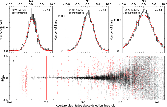
Figure 9. Aperture photometry demonstration. The plots show identical measurements to those in Figure 8, but for aperture photometry, as discussed in Section 4.8, rather than PSF photometry.
Download figure:
Standard image High-resolution imageWe largely attribute the behavior on the bright end to systematic errors in the photometry due to our inability to perfectly represent the shape of the PSF. The PSF of stars at the bright end will depend on the brightness because of the "Brighter-Fatter" effect (Antilogus et al. 2014; Gruen et al. 2015), in which the charge already present in the pixels will force the newly arriving photoelectrons to be systematically pushed away from the accumulating stellar image, but we do not include a brightness term in our PSF model. Detector or electronic nonlinearity may also affect the PSF shape and thus the PSF photometry, though nonlinearity will affect the reported photometry for both PSF and aperture magnitudes.
We believe the observed behavior at the faint end is primarily a result of the increased crowding. Aperture photometry is more adversely affected by close neighbors than PSF photometry. Compared to the formal errors, the faint PSF photometry is the most reliable, with the aperture photometry degrading rapidly as the flux of the star decreases.
The figures above show the relative photometric accuracy for observations at a consistent pointing compared to the photon-counting statistics. A related question is to ask how consistent is the photometry of the very brightest stars in terms of magnitudes. Figure 10 shows the accuracy of the brightest stars in these images for both PSF and aperture magnitudes. The relative zero-point between the first image in the sequence and each of the remaining images was calculated and the standard deviations were measured using stars 7 to 8 mag brighter than the detection threshold, for which the photon noise is less than 1 mmag. Significant zero-point differences between the images are observed, largely due to the atmospheric transparency variations. Even so, the relative zero-points calculated from the aperture magnitudes have standard deviations of 2.4–7.4 mmag with a median of 3.5 mmag, while for PSF magnitudes, the standard deviations are in the range 6.7–14.2 mmag, with a median of 9.2.

Figure 10. Demonstration of photometric accuracy using the image sequence from Figure 8. Using only bright stars (7–8 mag above the detection threshold), we calculate the difference between the magnitudes in the first image and the other 17 images. The plotted dots show for each pair the mean difference vs. the standard deviation of the difference. Red dots show the PSF magnitudes and blue dots show aperture magnitudes. Despite real transparency variations of 0.4 over the 50 minutes of this sequence, magnitudes are consistent at the few millimagnitude level. Aperture magnitudes have scatter in the 2–7 mmag range, while the PSF magnitudes have scatter of 7–14 mmag.
Download figure:
Standard image High-resolution imageOur ultimate ability to accurately measure the brightness of individual sources depends on a few factors: the accuracy of the flat-field response, the consistency of the flux measurement across the image (either due to the accuracy of the PSF model or the accuracy of the aperture correction), and the accuracy of our correction for any zero-point changes. Our ability to accurately measure the zero-point of each exposure depends in part on the characteristics of the observing site. In hazy conditions, the transparency of the atmosphere may vary substantially in time but be relatively stable across the field of view of the camera, as is shown in Figure 10. Conversely, thin patchy clouds can result in small average transparency changes but substantial localized variations. If the site experiences more patchy clouds than smooth haze, photometric calibration will be difficult. A large fraction of time with cloudless conditions will benefit the calibration.
To examine the Pan-STARRS site characteristics, we extracted  zero-points for the lifetime of the observatory (2009 June–2020 April), shown in Figure 11. These zero-points were measured as part of the PV3 analysis of the 3π Survey, and from the nightly data analysis after the end of the 3π Survey, in both cases using the Pan-STARRS-based reference catalog. The zero-points vary from night to night and over long periods. Over the 11 years of PS1 operation, the observed
  -band zero-point (for data in good weather, extrapolated to the zenith) has varied over 0.175 mag (see Figure 11). The long-term variations are believed to be due mostly to dust accumulation on the primary mirror and occasional cleaning, though the effect of the atmosphere cannot be ruled out.

Figure 11. Historical  -band zero-points. Blue dots are the individual exposure zero-points, corrected to airmass at the zenith. Red dots are the median of the zero-points from image groups in bins of 10 nights. The gray line is a spline fit to these median values.
Download figure:
Standard image High-resolution imageFigure 12 shows a log-scale histogram of the  -band zero-points after subtracting a smoothly varying spline fit to the median of groups of 10 nights. A Gaussian fit to this distribution has
  mmag. If we alternatively subtract a median zero-point for each night, the standard deviation is reduced to 17.6 mmag. These values can be compared to the results of Schlafly et al. (2012), in which only photometric nights were included, yielding a standard deviation of 9.0 mmag. On short timescales, weather (e.g., clouds & haze) causes the deviations to lower zero-point values. A small fraction of positive deviations also seen in Figure 12, which are not expected from the normal effects of weather. We believe these are largely due to aperture correction errors.
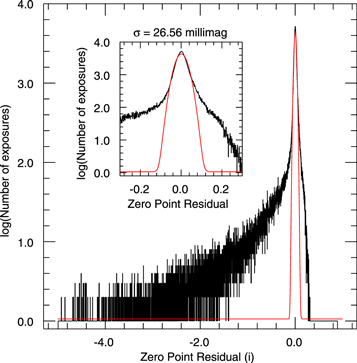
Figure 12. Historical  -band zero-point residual variations. Log-histogram (black line) of the per-exposure zero-points, corrected to the zenith, after subtracting a spline fit to the median of image groups in bins of 10 nights. The inset shows the core of the distribution. In both, the red line is a Gaussian fit to the distribution. The large negative tails are due to clouds and haze.
Download figure:
Standard image High-resolution image4.11. Basic Analysis Summary
This section is focused on the basic analysis of the image for point-source detection and measurement. This analysis is applied as described to the individual exposures in the chip-stage analysis and the measurements are exposed in the public release PSPS database in the Detection table. The same analysis is applied to the individual skycells in the stack-stage analysis and the resulting values are presented in the PSPS StackObjectThin and StackObjectAttribute tables, with the latter presenting values in instrumental units and the former giving calibrated values. The detection efficiency information determined from the injection and recovery analysis is stored in the ImageDetEffMeta and StackDetEffMeta tables for the chip- and stack-stage analysis.
5. Extended Source Analysis
After the initial, fast analysis of the image relying primarily on the PSF model, a complete analysis of the extended source properties may be performed. For PS1 processing, this step is skipped in the nightly (PV0) analysis of individual exposures and only performed for the stacks in the major reprocessing.
The extended source analysis consists of the following types of measurements: (1) an analysis of the radial profile of the surface brightness of the source, (2) measurement of the Petrosian radius and magnitude, (3) convolved galaxy model fits, and (4) photometry in several fixed-sized apertures, both raw and convolved to a defined PSF size. The motivation for these measurements is to provide options to the end users for galaxy photometry and reliable galaxy colors. The photometric redshift analysis of Saglia et al. (2012), for example, uses the convolved, fixed-size aperture photometry.
The extended source analysis is not applied to all objects which may be galaxies. Several restrictions are possible within the software. For example, it is possible to limit which objects are processed by their apparent magnitudes, by their signal-to-noise, by an indication if they are in fact extended, by the local stellar density, or by the galactic latitude. Some of these selections may be defined differently for the galaxy model fits and the Petrosian parameters.
For the 3π PV3 processing, both an apparent magnitude cut and a Galactic latitude cut were applied. The apparent magnitude limits for the galaxy model fits are applied to the measured Kron magnitude and depend on the filter as follows: ( ,
,  ,
,  ,
,  ,
,  ) = (21.5, 21.5, 21.5, 20.5, 19.5). These values were chosen to have roughly similar S/Ns in a typical stack image for objects with colors of typical galaxies. The magnitude limits for the Petrosian parameters were set to 25.0 for all filters, far below the detection limits and effectively not limiting the analysis based on apparent magnitude. For both galaxy model fits and Petrosian parameters, the Galactic latitude cut was defined by
  , where
  . For the PV3 analysis,
  20°,
20°,  15°,
15°,  50°. See Figure 13 for an illustration of the cut used for PV3. The Galactic plane cut is made on an object-by-object basis. This contour avoids the denser portions of the Galactic plane and bulge, limiting the total time spent on the galaxy modeling analysis at the expense of galaxy photometry in the plane (though Kron photometry is available for those sources).
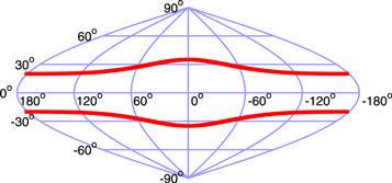
Figure 13. Illustration of the Galactic plane cut used for PV3, in Galactic coordinates. Objects within the red contours are skipped for galaxy model fits and Petrosian parameters.
Download figure:
Standard image High-resolution image5.1. Radial Profiles
Galaxies with regular profiles, such as elliptical galaxies and regular spiral galaxies, may be described as primarily a radial surface brightness profile, with additional structure acting as a perturbation on that profile. For many galaxies, the azimuthal shape at a given isophotal level may be described as an elliptical contour. To first order, a galaxy may be well described with a single elliptical contour and radial profile.
In order to facilitate the Petrosian photometry analysis below, psphot generates a radial profile for each suspected galaxy. This analysis starts by generating a radial profile in 24 azimuthal segments. Near the center of the galaxy, the profile is defined for radial coordinates in steps of 1 pixel, with the closest pixel values interpolated to that radial position. Further from the center, the profile is defined using the median of the pixels landing in an annular segment of size  , rounded up to the nearest integer pixel value. The median of all pixels within a rectangular approximation to the radial wedge is used.
The resulting 24 radial profiles are subject to contamination from neighboring sources or to NAN values from masked pixels. To clean the profiles, pairs of radial profiles from opposite sides of the source are compared. Any masked values are replaced by the corresponding value in the other profile. The minimum of both profiles is then kept for both profiles. The result of this analysis is a set of profiles of the form  . In this case, fi
is effectively the surface brightness for each radius in instrumental counts per pixel. If fewer than four radial surface brightness values are available for the analysis, the source is skipped and the flag bit PM_SOURCE_MODE2_ECONTOUR_FEW_PTS is set. Some apparently extended sources are in fact bright stars with a central saturation. These sources show up in this analysis as having many NAN-valued pixels in the central regions. During the radial profile analysis, such sources are flagged with the bit PM_SOURCE_MODE2_RADBIN_NAN_CENTER and are skipped from the rest of the analysis.
. In this case, fi
is effectively the surface brightness for each radius in instrumental counts per pixel. If fewer than four radial surface brightness values are available for the analysis, the source is skipped and the flag bit PM_SOURCE_MODE2_ECONTOUR_FEW_PTS is set. Some apparently extended sources are in fact bright stars with a central saturation. These sources show up in this analysis as having many NAN-valued pixels in the central regions. During the radial profile analysis, such sources are flagged with the bit PM_SOURCE_MODE2_RADBIN_NAN_CENTER and are skipped from the rest of the analysis.
The surface brightness profiles are then used to define the azimuthal contour at a specific isophotal level. This contour will be used to rescale the radial profiles into a single set of profiles normalized by the elliptical contour. This contour is defined by determining the median radius for profile bins with surface brightness in the range  to
to  . The result of this analysis is a value for the radius as a function of the angle for a well-defined surface brightness regime. We then determine the elliptical shape parameters for this elliptical contour:
  . This ellipse is then used to redefine a single radial profile normalized by the elliptical contour:
The surface brightness values are sampled at a number of radial annuli, with the radii defined in the configuration (RADIAL.ANNULAR.BINS.LOWER & RADIAL.ANNULAR.BINS.UPPER). For each source, the resulting surface brightness profile is saved in the output FITS table as a vector (PROF_SB). The flux at each radial position and the fill factor (fraction of pixels used to the total possible) are also saved as equal-length vectors in the FITS table (PROF_FLUX and PROF_FILL). The values of the radial bins are saved in the output file FITS header (RMIN_NN, RMAX_NN). These measurements are saved in the catalog FITS files generated by psphot, but they are not currently exported to the PSPS database for easy access.
5.2. Petrosian Radii and Magnitudes
Petrosian (1976) defined an adaptive aperture based on a ratio of surface brightnesses. The motivation is to define an aperture that can be determined for galaxies without significant biases as a function of distance from the observer. As the surface brightness profile in a resolved source is conserved as a function of distance, using a ratio of surface brightness to define a spatial scale results in a spatial scale that is constant regardless of galaxy distance.
To measure the Petrosian radius and flux, we start by defining a series of radial apertures with power-law spacing:  . We calculate the surface brightness for the annulus from
  by calculating the median of the values in the range
  to
to  and dividing the effective area of the annulus corresponding to
  .
.
For any annulus i spanning the radii  to
to  , the Petrosian ratio for that annulus is defined as the ratio of the surface brightness in the annulus to the average surface brightness within
  . The Petrosian radius is defined to be rmax for the annulus for which the Petrosian ratio = 0.2, i.e., the point on the galaxy radial profile at which the surface brightness is 20% of the average surface brightness at that point. If the profile falls below the Petrosian ratio for the first radial bin, the flag bit PM_SOURCE_MODE2_PETRO_RATIO_ZEROBIN is set to note that the Petrosian radius may be poorly determined.
We determine the Petrosian radius for the galaxy by quadratic interpolation between the last two of the fixed annuli with Petrosian ratio  and the first annulus with Petrosian ratio
  . In general, the Petrosian ratio for a galaxy with a regular morphology (spiral or elliptical) is falling monotonically, so this interpolation is unambiguous. However, irregular galaxy morphologies, noise, and/or significant masking can cause the Petrosian ratio to have rises as well as drops. We track the Petrosian ratio until the value is no longer significant (
 ). If the Petrosian ratio drops below 0.2 for more than one radius, we choose the largest such radius. If the Petrosian ratio does not fall below 0.2 for any of the measured radii, we choose the annulus for which the ratio falls to the lowest (yet still significant) value. In such a case, the flag bit PM_SOURCE_MODE2_PETRO_INSIG_RATIO is set.
Once the Petrosian radius has been determined, we can now measure the Petrosian flux: this is defined to be the total flux within an aperture corresponding to 2× the Petrosian radius. Using the Petrosian flux, we can calculate two other interesting radii: R50 and R90, the radii inside which 50% and 90% of the total Petrosian flux is contained. Sources for which the Petrosian parameters are successfully measured have the flag bit PM_SOURCE_MODE_EXTENDED_STATS set. Sources for which the Petrosian parameters were attempted but for which the radial profile analysis failed have the flag bit PM_SOURCE_MODE2_PETRO_NO_PROFILE set. These measurements are available from the PSPS StackPetrosian table.
Our implementation of the Petrosian apertures and fluxes is designed to match the SDSS implementation (Stoughton et al. 2002), and therefore, the measured parameters should be quite comparable between the two surveys. Figure 14 compare the Petrosian magnitudes and radii as measured by psphot on the 3π Survey observations and the values measured by SDSS for the same objects. Objects identified by SDSS as galaxies (probPSF_r
 ) near the Galactic north pole (α = 180° to 190°s, δ = 25° to 35°s) are selected from the PS1 3π Survey data set base on positional coincidence. The figure shows the difference in the r-band Petrosian magnitudes as a function of the Petrosian magnitude and as a function of the difference in the measured Petrosian radii. Differences in the measured magnitudes are driven by differences in the size estimates from the two data sets and analysis methods. The PS1 analysis tends to find larger radii than the SDSS analysis for the same objects, with a mean difference of 03. The larger aperture results in more flux captured in the aperture and thus brighter magnitudes for the same object: the mean difference is –0.23 magnitude in the sense of larger fluxes for the PS1 measurements.
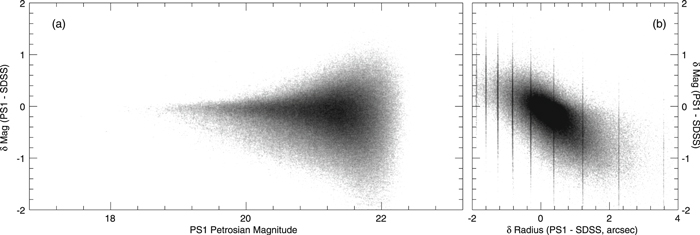
Figure 14. Comparison of PS1 (psphot) and SDSS Petrosian parameters for objects identified as galaxies by SDSS. Panel (a) shows the difference in the measured Petrosian magnitudes as a function of the Petrosian magnitude. Panel (b) shows the magnitude difference as a function of the measured difference in the Petrosian radius.
Download figure:
Standard image High-resolution image5.3. Convolved Galaxy Model Fits
In the galaxy model-fitting stage, sources that meet certain criteria are fitted with analytical models for galaxies. Three traditional analytical galaxy models are implemented in psphot and used in the PV3 analysis:


where ρ is a normalized radial term:  . The terms (Rxx
, Ryy
, Rxy
) describe the elliptical contour and the profile scale in all three models and the coordinates x and y are determined relative to the centroids (
. The terms (Rxx
, Ryy
, Rxy
) describe the elliptical contour and the profile scale in all three models and the coordinates x and y are determined relative to the centroids ( ). Including the normalization (I0) and a local sky value, the Exponential and de Vaucouleur profiles have seven free parameters and the Sérsic profile has the additional free parameter of the Sérsic index n. In this stage, the galaxy model is convolved with an approximation to our best guess for the PSF model at the location of the galaxy.
Sources that passed the extended source restrictions described above were fitted with all three galaxy models, unless (a) the morphological test identified the source as a likely cosmic ray (Section 4.6.5) or (b) the peak of the PSF profile was above the saturation limit for the chip (see the discussion in Waters et al. 2020, regarding the masking of saturated pixels). For all sources for which the extended source model fits were attempted, the flag bit PM_SOURCE_MODE2_EXT_FITS_RUN is set. If any of the attempted model fits failed, then the flag bit PM_SOURCE_MODE2_EXT_FITS_FAIL is set. If all model fits failed, then the flag bit PM_SOURCE_MODE2_EXT_FITS_NONE is set.
Before the nonlinear fitting may be performed, it is necessary to determine initial values for the parameters to be fitted. For each of the three model types, the position determined from the PSF fitting analysis is used as the initial centroid  . A guess for the terms (Rxx
, Ryy
, Rxy
) is generated based on the second moments. The guess does not attempt to use the PSF model to adjust the (Rxx
, Ryy
, Rxy
) values; it was found that such a guess tended to be too small and resulted in more iterations rather than fewer. The first radial moment (see Section 4.4.3) is used to estimate the effective radius of the model based on the results of (Graham & Driver 2005, Table 1). They quantify the relationships between the first radial moment used to calculated a Kron magnitude and the effective radius for different Sérsic index values, n. Because the Exponential and de Vaucouleur models are equivalent to Sérsic models with n = 1 and 4, respectively, this work can be used to generate the initial effective radius values for all three model types. Once the effective radius is chosen, the second moments are used to define the aspect ratio and position angle of the elliptical contour, as described for PSF sources in Section 4.5.3. The Kron flux is used to generate a guess for the normalization, applying an appropriate scale factor based on the (Rxx
, Ryy
, Rxy
) values, generated by integrating normalized Sérsic models and determining the relationship between the central intensity and the integrated flux as a function of the Sérsic index.
. A guess for the terms (Rxx
, Ryy
, Rxy
) is generated based on the second moments. The guess does not attempt to use the PSF model to adjust the (Rxx
, Ryy
, Rxy
) values; it was found that such a guess tended to be too small and resulted in more iterations rather than fewer. The first radial moment (see Section 4.4.3) is used to estimate the effective radius of the model based on the results of (Graham & Driver 2005, Table 1). They quantify the relationships between the first radial moment used to calculated a Kron magnitude and the effective radius for different Sérsic index values, n. Because the Exponential and de Vaucouleur models are equivalent to Sérsic models with n = 1 and 4, respectively, this work can be used to generate the initial effective radius values for all three model types. Once the effective radius is chosen, the second moments are used to define the aspect ratio and position angle of the elliptical contour, as described for PSF sources in Section 4.5.3. The Kron flux is used to generate a guess for the normalization, applying an appropriate scale factor based on the (Rxx
, Ryy
, Rxy
) values, generated by integrating normalized Sérsic models and determining the relationship between the central intensity and the integrated flux as a function of the Sérsic index.
The PSF-convolved galaxy model fitting analysis uses the Levenberg–Marquardt minimization method to determine the best fit. In this process, the  value to be minimized is
where Ip
represents the pixel values in the image (within some aperture) and  represents the unconvolved galaxy model, a function of a number of parameters
  , which is then convolved with the PSF model.
To determine the minimization, we need the gradient and Laplacian of  with respect to the model parameters, am
:
with respect to the model parameters, am
:


where we define
and we have approximated the Laplacian with the Hessian matrix,  , by dropping the second derivatives (which are assumed to be a small perturbation).
Because
and because the order of the derivative and convolution may be exchanged, we can write these in terms of the convolved image of the model and the convolved images of the derivatives of the model Mp with respect to the model parameters, am :

The gradient vector and Hessian matrix are used in the Levenberg–Marquardt minimization analysis using the standard technique of determining a step from the current set of model parameters to a new set by solving the matrix equation:
where  is zero for
  and for m = n set to be large when the last iteration produced a large change in the parameters compared to the local linear expectation and small when the last change was small. The iteration ends when the change in the parameters is small or the change in the
  value is small.
In the analysis, convolved galaxy fits, the galaxy model image, and the model derivative images must be convolved with the PSF at each iteration step. To save computation time, this convolution is performed using a circularly symmetric approximation of the PSF model, with the PSF model scale size set to the average of the major and minor axis direction scale size of the full PSF model, with the same radial profile term as the PSF model. The convolution is performed directly using the circular symmetry to reduce the number of multiplications performed: all points in the 2D circularly symmetric PSF model that have the same radial pixel coordinate can be evaluated in the convolution by summing up the corresponding pixels in the (galaxy model) image to be convolved before multiplying by the PSF model profile at that radial coordinate. This approximation reduces the number of multiplications by a factor of ∼8 for larger radii. For the small size of the PSF model used to convolve the galaxy model images, it was found that this direct convolution was faster than using an FFT-based convolution.
For the Exponential and de Vaucouleur fits, all parameters are fitted in the nonlinear minimization stage. For the Sérsic model, we do not fit the index within the Levenberg–Marquardt analysis. Instead, we start with a coarse grid search over a range of possible index values ( ) and a range of possible values for
  based on the value of R1, the first radial moment. For a given value of the Sérsic index, the
  is related to the first radial moment by the scale factor specified by Graham and Driver. We use the observed value of the 1st radial moment and try
  values of a factor of (0.8, 0.9, 1.0, 1.12, 1.25) times the value predicted by the Graham and Driver equation. For each of these steps, the aspect ratio and position angle are held constant and the normalization is determined to minimize the
  .
.
We next perform three Levenberg–Marquardt minimization fits allowing the shape parameters (Rxx
, Ryy
, Rxy
) and the normalization to be fitted, holding the centroid ( ), Sérsic index n and sky constant. In these fits, the index n is set to the minimum value previously calculated as well as values halfway to the next, and previous, values in the grid above. For example, if the minimum fitted index value is 3.0, then the LMM fits are performed using n = 2.5, 3.0, 3.5. The resulting
  values are then used to perform quadratic interpolation to find the index n which produces the locally minimum
  value. Finally, this best-fit index value is held constant while Levenberg–Marquardt minimization is used to find the best fit values of all other parameters. Sources for which a convolved galaxy model fit was successful have the flag bit PM_SOURCE_MODE_EXTENDED_FIT set.
The central pixel of the Sérsic, de Vaucouleur, and Exponential models requires special handling. When comparing an analytical model to the pixelized image recorded by a CCD, one normally treats the value in a pixel as equivalent to the value of the model at the center of the pixel. However, in reality, the number of counts observed in a pixel represents the integral of the surface brightness across the area of the pixel. This average will be equal to the central surface brightness times the area of a pixel as long as the second and higher derivatives of the analytical model are zero. However, if the first and second derivatives are nonzero, the curvature of the function within the pixel will make the integral differ from the central surface brightness times a fixed pixel area. If the curvature of the model function is sufficiently large, this difference will have a significant impact on the evaluation of the model. This situation is particularly true for the central portion of the Sérsic-like model functions.
In order to accurately compare the observed galaxy flux distribution to a model, it is necessary to integrate the pixel flux for a given set of model parameter values. In the psphot implementation, we currently use a brute-force numerical evaluation of the integral, dividing the central pixel into a grid of subpixels, with the sampling set by the Sérsic index of the model being evaluated as  , where
  is the subpixel scale n is the Sérsic index and
  is the size of the minor axis in pixel units. The value of
  is constrained to be in the range 11 to 121, so the number of subpixel evaluations ranges from 121 to
  . Faster approximations to this analysis were explored, but they resulted in unsatisfactory results. This is definitely an area where psphot could benefit from some of the lessons in the literature (e.g., Hogg & Lang 2013).
The convolved galaxy model fit results are available in one of three PSPS database tables: StackModelFitExp, StackModelFitDeV, StackModelFitSer for the Exponential, de Vaucouleur, and Sérsic models, respectively.
5.4. Fixed-aperture Photometry
For some science goals, a well-measured color of a galaxy is more important than an accurate total magnitude. In the case of PS1, the image quality variations for stacks of different filters presents a serious challenge for the determination of precise colors. psphot determines a set of PSF-matched radial aperture flux measurements in order to minimize the impact of the stack image quality variations.
In psphotStack, the stack analysis version of psphot, the five filter images are processed together. After the PSF models have been fitted and a best set of galaxy models have been determined, three sets of fixed circular apertures are measured. In the first set, the fluxes in the apertures are measured using the raw stack images. The centers of the apertures for each source across the five filters are fixed so that the pixels represent the equivalent portions of the same galaxy for all five filters. In this analysis, the best model for each source is subtracted from the image pixels for all sources excluding the source in consideration. The "best model" is determined based on the minimum  value for the model fits.
In addition to the raw fixed circular apertures, the stack images are each convolved with a circular Gaussian with σ chosen to yield an image with a typical FWHM of 6 pixels (15). The full set of circular apertures is again measured on these convolved images. Again, the best source models are subtracted from the image for sources not being measured. This subtraction includes the convolution to smooth the model to the effective FWHM of the convolved image. The entire procedure is then repeated with a target FWHM of 8 pixels (2''). Note that we do not attempt to restrict the stack image quality to match these convolution targets. If the stack has an effective FWHM larger than either the 6 or 8 pixel targets, the convolution does not take place and the resulting analysis is performed on the raw stack. In such cases, the smallest apertures are sensitive to seeing variations and should be avoided. Of the individual images, the fraction with FWHM larger than 8 pixels is ( ,
,  ,
,  ,
,  ,
,  ) = (9.8%, 5.1%, 4.9%, 3.4%, 3.7%), and the fraction of stacks with an effective FWHM larger than this limit will be much smaller.
For the PV3 analysis of the 3π Survey data, the fluxes are measured for a set of up to nine circular apertures with sizes chosen to match the similar circular apertures measured by the SDSS analysis. These apertures have radii of (4.16, 7.04, 12.0, 18.56, 29.76, 45.68, 72.80, 112.80, 176.88) pixels = (104, 176, 300, 464, 744, 1142, 1820, 2820, 4422). If the object is too faint, the larger apertures will be largely noise, and the computation is wasteful. We only calculate the circular apertures out to the second aperture larger than the "sky radius" (defined in Section 4.6.3), but we calculate photometry for at least the smallest four apertures. Sources for which photometry in these fixed aperture is calculated have the flag bit PM_SOURCE_MODE_RADIAL_FLUX set. Although these apertures are chosen to match the SDSS apertures, the SDSS images are measured on unconvolved images. Because the median seeing for the SDSS images is ∼14 in the r band (Adelman-McCarthy et al. 2007), our 15 aperture photometry should generally compare well to the SDSS aperture magnitudes.
The measurements described in this subsection are presented in the PSPS database (Paper VI) in the StackApFlxExGalUnc, StackApFlxExGalCon6, StackApFlxExGalCon8, and StackApFlx tables. The first three tables present measurements for all apertures from the unconvolved, and 6 and 8 pixel FWHM convolved images (respectively) while the last table presents a subset of the radii from all three sets of measurements joined together for ease of access.
5.5. Galaxy Model Simulations
To test the galaxy model analysis, we have generated a series of simulated images containing both stars and galaxies on which we have run the psphot PSF-convolved galaxy model fitting analysis. The images generated for this analysis have dimensions of 4000 × 4000 pixels with a spatial scale of 025 per pixel. The images are generated using an effective exposure time of 30 s, with zero-points matching the PS1  filter and a realistic sky brightness of 20.86 mag per arcsec2. The stars are injected into these images with fluxes drawn from a realistic stellar luminosity function and random spatial locations. For each image, the same underlying simulated stellar population was used. Galaxies are injected into the image with positions on a regularly spaced grid with a separation of 120 pixels. A total of 1089 galaxies are injected in each image, with all galaxies in an image having the same total magnitude. Galaxies were injected for 51 magnitude bins, ranging from 17.0 to 22.0. Given the parameters of the image, these values span the range from high S/N (
 ) to undetectable (S/N < 1). Note that we are not attempting to represent a realistic astronomical distribution of galaxies but rather attempting to understand our ability to recover galaxies of a certain type, size, and shape in a given image.
The galaxies are injected using Exponential and de Vaucouleur profiles in separate simulation runs. The major-axis values are randomly distributed between 1 and 10 pixels (025–25) while the aspect ratios are randomly chosen in a range from 0.25 to 1.0. The position angles are set by the sequence in the image and allowed to vary from 0° to 180°. The images are then convolved with a circular PSF model using the PS1_V1 profile (FWHM = 10,  ), and noise is added using Poisson statistics for the detected photons.
For the figures below, we present results as a function of the (input) instrumental magnitude of the galaxy minus the instrumental magnitude corresponding to the stellar 5σ detection limit. We make the simplifying assumption that the stellar detection threshold encapsulates enough information about the sensitivity of the images that this magnitude difference may be used to compare the results shown here to images with other depths. Thus, this and subsequent figures may be compared with the reported detection limits from the PS1 3π Survey. Note for reference that the typical stellar detection limits in the PS1 3π stack images (Paper I) are ( ,
,  ,
,  ,
,  ,
,  ) = (23.3, 23.2, 23.1, 22.3, 21.4). The minimum Kron magnitudes for which galaxy model fits were performed for the PV3 analysis (Section 5) thus correspond to −1.6 to −1.8 in these plots.
Figure 15 shows completeness for the detection of the Exponential and de Vaucouleur model galaxies. This analysis does not indicate if the galaxy was detected as a galaxy (i.e., was the extended nature of the source sufficiently clear), only if the source was detected by the peak-finding algorithm. As expected, the more compact galaxies are more likely to be detected; Exponential profile galaxies, with a broader light distribution for the same effective radius, are less likely to be detected for the same magnitude than de Vaucouleur profile galaxies. This completeness should be compared to our earlier work (Metcalfe et al. 2013) in which we injected a realistic population of simulated galaxies into real PS1 images. That work found that the 50% completeness for the typical galaxy was roughly 0.5 mag brighter than the 50% stellar completeness limit, somewhat fainter than the completeness shown in Figure 15. However, that previous work did not explore the dependency of the completeness on the galaxy size or profile. The difference suggests that the galaxies in the earlier work were generally compact.

Figure 15. (a) Completeness curves for simulated galaxies with Exponential profiles. (b) Completeness curves for simulated galaxies with de Vaucouleur profiles. The curves are shown as a function of the difference between the injected instrumental magnitude of the galaxy and the magnitude corresponding to the 5σ detection threshold for a PSF-like source. The black curves show the completeness for all galaxies. The three colored curves show the completeness for three major-axis ranges. Compact galaxies are more likely to be detected since peaks are detected after convolution with the PSF. The simulated images have seeing of 1'', equal to pixels.
Download figure:
Standard image High-resolution imageFigures 16 and 17 demonstrate the recovery of galaxy parameters in these simulations for galaxy using the Exponential and de Vaucouleur models, respectively. Both figures show the reliability of the measured magnitudes, major and minor axis sizes, and ellipticities, which we represent as  . Galaxies are grouped in 0.1 mag bins based on their injected magnitudes. For all recovered parameters, the standard deviation of the difference between the measured parameter and the truth value is shown for all galaxies in each magnitude bin, as well as for subsets in major-axis ranges. The mean of the difference, illustrating any biases, is also given for all galaxies. The comparison for the major and minor axis sizes are shown as absolute measurements (in pixels) and as a fraction of the axis in question.

Figure 16. Parameter recovery for simulated galaxies with Exponential profiles. In each panel, we show several statistics for the difference between the truth parameter and the measured value for galaxies in a series of brightness bins, ranging from 5 mag to 0.5 mag brighter than the PSF 5σ detection threshold. Statistics, as shown in the legend, include the average difference, the standard deviation for all galaxies in the bin, and the standard deviations for three major-axis ranges. Panels (a)–(d) show in order the recovered magnitudes, ellipticity, major-axis size, and minor axis size. Panels (e) and (f) show statistics for the major and minor axis difference as a fraction of the truth value. The average magnitude difference is plotted so that positive numbers mean the fitted flux is brighter than the injected flux.
Download figure:
Standard image High-resolution image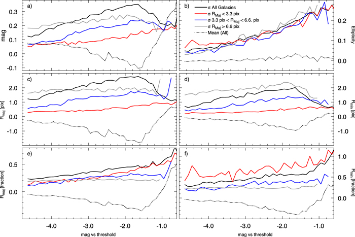
Figure 17. Parameter recovery for simulated galaxies with de Vaucouleur profiles. See Figure 16 for a complete explanation.
Download figure:
Standard image High-resolution imageSome overall patterns can be observed. First, the parameters measured for the exponential profile galaxies are consistently more reliable than those measured for the de Vaucouleur profiles. Second, the errors in the estimated magnitudes are primarily driven by errors in the size measurements: if the sizes are overestimated, the fluxes are also overestimated. Finally, the magnitudes and major axes are more accurate for the smaller galaxies, but the ellipticities are more accurate for the larger galaxies.
6. Forced-warp Analysis
Traditionally, projects that use multiple exposures to increase the depth and sensitivity of the observations have generated something equivalent to the stack images produced by the IPP analysis, as done for example by the Canada–France–Hawaii Telescope (CFHT) Legacy Survey (Hoekstra et al. 2006) or the Cosmic Evolution Survey (COSMOS; Capak et al. 2007). In theory, the photometry of the stack images produces the "best" photometry catalog, with best sensitivity and the best data quality at all magnitudes (see, e.g., the discussion in Zackay & Ofek 2017). In practice, these images have some significant limitations due to the difficulty of modeling the PSF variations. This difficulty is particularly severe for the Pan-STARRS 3π Survey stacks due to the combination of the substantial mask fraction of the individual input exposures, the large intrinsic image quality variations within a single exposure, and the wide range of image quality conditions under which data were obtained and used to generate the 3π PV3 stacks.
For any specific stack, the PSF at a particular location is the result of the combination of the PSFs for those individual exposures that went into the stack at that point. Because of the high mask fraction, the exposures that contributed to pixels at one location may be somewhat different just a few tens of pixels away. In the end, the stack images have an effective PSF that is not just variable, but changing significantly on small scales in a highly textured fashion.
Any measurement that relies on a good knowledge of the PSF at the location of an object needs to determine the PSF variations present in the stack image or the measurement will be somewhat degraded. The highly textured PSF variations make this a very challenging problem: not only would such a PSF model require an unusually fine-grained PSF model, there would likely not be enough PSF stars in a given stack image to determine the model at the resolution required. The IPP photometry analysis code uses a PSF model with 2D variations using a grid of at most 6 × 6 samples per skycell, a number reasonably well matched to the density of stars at most moderate Galactic latitudes. This scale is far too large to track the fine-grained changes apparent in the stack images.
As a result, PSF photometry as well as convolved galaxy models in the stack are degraded by the PSF variations. Aperture-like measurements are in general not as affected by the PSF variations, as long as the aperture in question is large compared to the FWHM of the PSF.
The IPP analysis solves this problem by starting with the sources detected in the stack images and performing a highly constrained analysis on the individual warp images used to generate the stack and then combining the resulting measurements to determine a high-quality average value. We consider all of these measurements to be "forced" because of the strong prior constraints from the stack. This analysis is performed using the psphotFullForce variant of psphot.
6.1. Forced PSF Photometry
PSF photometry is measured for all objects detected in the stack using the positions determined by the stack photometry analysis. Candidate PSF stars are pre-identified as those stars used to generate the PSF model in the stack photometry analysis. A PSF model is generated for each input warp image based on those stars; PSF stars that are excessively masked on a particular image are not used to model the PSF. The normalization of the PSF model is fitted to all of the known source positions in the warp images to determine the PSF fluxes. This measurement is performed simultaneously for all sources in the image at once using the method described above (Section 4.6.2).
Aperture fluxes, Kron fluxes, and moments are also measured at this stage for each warp. For the Kron fluxes, the radii are fixed to the value determined in the analysis of the stack. Fluxes are also measured in three of the fixed apertures discussed in Section 5.4: those with 300, 464, and 744 radii. Note that the flux measurement for a faint, but significant, source from the stack image may be at a low significance (less than the 5σ criterion used when the photometry is not run in this forced mode) in any individual warp image; the measured flux may even be negative due to statistical fluctuations. When combined together, these low-significance measurements result in a significant measurement as the S/N increases with the combination of more data.
Individual warp images are processed independently with separate executions of the psphotFullForce program. Sources that are loaded by psphotFullForce for analysis are marked with the flag bit PM_SOURCE_MODE_EXTERNAL. This bit is also used to mark user-supplied sources loaded for analysis by the regular version of psphot. Once all of the forced photometry measurements (for point sources as well as galaxies, discussed below) are completed for all of the warps that contributed to a stack image, the measurements are combined together by other portions of the IPP system. The PSF photometry measurements are combined in the context of the DVO database system (Magnier et al. 2020a), including recalibration of the zero-points for the individual warps. These measurements for each warp are available from the PSPS database ForcedWarpMeasurement and ForcedWarpExtended tables, the latter containing the three fixed-aperture fluxes. The average values calculated over the warps are found in the ForcedMeanObject tables.
With the inclusion of the forced-warp photometry, we have three distinct methods for measuring the PSF photometry of stars in the Pan-STARRS survey data: the average of the chip-stage photometry from the individual exposures, the measurement from the stacks, and the average of the forced-warp photometry described here. It is worth considering which of these should be used in which circumstance. Figure 18 shows a comparison of these three different methods to deeper data from the Medium-Deep Survey observations (MD06 field). Our conclusion from this and other analysis is that the average chip-stage photometry is the best (most accurate) measurement for brighter objects, where the signal-to-noise is roughly 10 or more. This is the photometry source that was used for the global photometry solution discussed by Schlafly et al. 2012 and used in the overall calibration (see Paper V).

Figure 18. Comparison of psphot average chip photometry (a), average forced-warp photometry (b), and stack photometry (c) from 3π Survey data to average forced-warp photometry from the Pan-STARRS 1 Medium-Deep Survey field MD06. At bright magnitudes, average chip photometry is most accurate while the stack photometry is degraded by the highly textured PSF. At faint magnitudes, average chip magnitudes are biased to artificially bright values.
Download figure:
Standard image High-resolution image
As can be clearly seen in the figure, the average from the forced-warp photometry is slightly worse than the chip photometry, while the stack PSF photometry is significantly degraded. We attribute the latter effect to the highly textured PSF observed in the stack images due to the combination of variable PSFs in each exposure and significant masking fraction in the PS1 camera. At the faint end, the chip photometry is significantly worse than both average warp and stack photometry. First, in order to have a measurement, a source must be detected above the detection threshold in at least one of the exposures, limiting the depth possible of the average chip photometry. Second, at the faint end, only bright fluctuations will be detected, resulting in a bright bias, a form of Eddington bias (Eddington 1913). This latter effect is clearly seen in Figure 18 as the average chip magnitudes diverge from the deeper Medium-Deep photometry measurements. As has been noted elsewhere (Best et al. 2018), the warp and stack photometry is also degraded for objects that have significant proper motion over the course of the 3π Survey because the position is held constant for all epochs, while the average chip photometry is calculated on detections that are cross-matched in the database. Thus, warp and stack photometry should be avoided for sources with proper motion greater than roughly 100 mas per year.
6.2. Forced Galaxy Models
The convolved galaxy models are also remeasured on the warp images by the psphotFullForce analysis. In this analysis, the galaxy models determined from the stack image analysis are used to seed the analysis in the individual warp images. The motivation of this analysis is the same as the forced PSF photometry: the PSF of the stack image is poorly determined due to the masking and PSF variations in the inputs. Without a good PSF model, the PSF-convolved galaxy models are of limited accuracy.
In the forced galaxy model analysis, we assume that the galaxy position and position angle, along with the Sérsic index if appropriate, have been sufficiently well determined in the analysis of the stack image. In this case, the goal is to determine the best values for the major and minor axes of the elliptical contour and at the same time the best normalization corresponding to the best elliptical shape, and thus the best galaxy magnitude value. This technique is similar to the joint fitting of multiple exposures performed by the CFHT Lensing Survey team (Miller et al. 2013).
For each warp image, the stack values for the major and minor axes are used as the center of a grid search of the major and minor axis parameter values. The grid spacing is defined as a function of the S/N of the galaxy in the stack image so that bright galaxies are measured with a much finer grid spacing than faint galaxies. For the PV3 3π analysis, a 5 × 5 grid was used; values in both the major and minor axis directions of  ,
,  , 1.0,
  ,
,  times the dimension are tested. For each grid point, the major and minor axis values at that point are used to generate the model. The model is then convolved with the PSF model for the warp image at that point. The resulting convolved model is then compared to the warp pixel data values and the best-fit normalization value is determined. The integrated flux, flux error, and the
  value for each grid point are recorded. This analysis is performed on the warp images one object at a time with the other objects in the image subtracted according to the best model currently known.
For a given galaxy, the result is a collection of  values, fluxes, and flux errors for each of the grid points spanning all warp images. A single
  grid can then be made by combining each grid point across the inputs. The combined
  for a single grid point is simply the sum of all
  values at that point. If, for a single warp image, the galaxy model is excessively masked, then that image will be dropped for all grid points for that galaxy. The reduced
  values can be determined by tracking the total number of pixels used across all inputs to generate the combined
  values. From the combined grid of
  values, the point in the grid with the minimum
  is found. Quadratic interpolation is used to determine the major, minor axis values for the interpolated minimum
  value. The errors on these two parameters are then found by determining the contour at which the
  increases by 1.
In this way, the forced galaxy model analysis uses the PSF information from each warp image to determine a best set of convolved galaxy models for each galaxy model measured for the stack image. The results of these galaxy model fits are available from the PSPS database ForcedGalaxyShape table.
6.3. Galaxy Lensing Parameters
Weak-lensing studies frequently use nonparametric measurements of the ellipticities of galaxies to quantify the strength of gravitational lensing, and thus directly measure mass distributions in the universe. The classic approach was originally described by Kaiser et al. (1995, hereafter KSB), and applied to a set of deep HST observations. The details of the technique were further refined by Hoekstra et al. (1998, hereafter HFK); in the discussion below, we primarily use their notation, though we explicitly cast their integrals as sums over discrete pixels.
The KSB-style analysis of object ellipticities has also been used by several authors to search for marginally resolved binary stars in wide-field imaging data. The use of the lensing statistics for this application was described by Hoekstra et al. (2005) in the context of vetting planet transit events in data from the Optical Gravitational Lensing Experiment (OGLE). Terziev et al. (2013) applied the technique to PTF data to search for binary stars and Deacon et al. (2017) used the same technique to search for binary companions to known ultracool dwarfs using Pan-STARRS 3π data. The work by Deacon et al. (2017) used images and their own analysis of the pixels with the program Sextractor (Bertin & Arnouts 1996).
For the Pan-STARRS 3π PV3 analysis, we have measured the full set of KSB lensing parameters for all objects with measured second moments (i.e., excluding saturated stars, suspected cosmic rays, and other likely defects) of the data to enable both lensing studies and binary/multiple star searches. Here, we describe the measurements as performed within psphot, reviewing the mathematical framework as described by KSB and HFK. Just like the forced PSF photometry and the constrained galaxy models above, this analysis is performed by measuring the KSB lensing parameters on the individual warp images and averaging these measurements for each object.
The goal of the KSB technique is to measure the intrinsic ellipticity of objects (i.e., galaxies, in the case of weak lensing studies) as would be observed on the sky on the without instrumental effects and to determine the impact weak gravitational lensing would have on the observed shapes, after correcting for the instrumental effects. The analysis starts with the observed ellipticity of objects as represented by the two polarization components derived from the second moments (see Section 4.4.3):
These two quantities have values that range from −1 to +1, with a circularly symmetric object having  . The two polarization components vary sinusoidally with twice the position angle of the object: an elongated object aligned with the x-pixel axis will have positive values of e1 and e2 values near zero, while the same object aligned with the y-pixel axis will negative e1 values. An object with a position angle on the 45° lines between the pixel axes will have large positive or negative values of e2 and low absolute values of e1.
Note that in our analysis of the second moments, we are applying a Gaussian window function to down-weight the noise contributions from pixels at high radii and low flux (see Section 4.4.3). This type of window function is also assumed in the KSB formalism and is represented in the equations below as W.
The measured ellipticity of an object observed in a real instrument will be affected by the PSF of the instrument. To first order, the effect on the polarization components can be described as a combination of the circularly symmetric seeing disk, which smears the observed shapes (driving  to low absolute values) and the shearing effect of the anisotropic component of the PSF, in which the observed shape is stretched in one direction relative to the others (driving
  to larger absolute values).
KSB and HFK quantify the change in the observed polarization due to the smearing effect of the PSF with

pβ
is a measurement of the anisotropy of the PSF (see below), and  is the "smear polarizability" of the object, defined as

where


and


In these equations,  and W is the window function applied when measuring the second moments. The terms
  and
and  are the derivatives of the window function with respect to
  . Because the window function is a circularly symmetric Gaussian with width
  , the derivatives are simply
  and
and  .
.
The elements of the equations above can be written in terms of the second- and higher-order moments calculated in Section 4.4.3:
and
where  .
.
KSB and HFK use the observed ellipticities of stars and the smear polarizability of the stars to estimate the anisotropy due to the PSF:
where the terms with the ∗ represent parameters measured on stars.
Similarly, the impact of shear can be quantified by the "shear polarizability" in a similar fashion:

where now the shear polarizability  is defined as

where


and


Rewriting in terms of the second- and higher-order moments calculated in Section 4.4.3, we find
and
In the Pan-STARRS PV3 analysis, we have measured the elements of the smear polarizability ( ,
,  ) and the shear polarizability (
 ,
,  ) for all objects on each of the warp images. We have also selected only the PSF stars from the images and interpolated a smoothed version of these parameters from the PSF stars to the locations of all objects, using the grid described above to interpolate the parameters. We then determine the ellipticities of the stars (
 ) from the equivalent smooth grid. Thus, for every object in the 3π Survey, we are able to report the PSF and object elements of the KSB analysis. These lensing parameters are measured for each of the warps, and then averaged over all warps for each of the filters. The average values are calculated by including only measurements from the same warp detection used in the average photometry (nominally, the primary skycell; see Paper V, Section 5.4.4) and excluding any measurements for which the PSF_QF or PSF_QF_PERFECT is less than 0.85.
The lensing parameters measured for individual warps are available from the PSPS database ForcedWarpLensing table while the average values calculated over the warps is found in the ForcedMeanLensing tables. Although the software used here was not involved in any of the GRavitational lEnsing Accuracy Testing (GREAT) challenges, it is similar to the code of the EPFL_KSB team (Mandelbaum et al. 2015) and likely to perform similarly.
7. Difference Image Photometry
Among the primary science drivers for Pan-STARRS are the detection of moving objects (e.g., asteroids) and explosive transient sources (e.g., supernovae). For both of these situations, difference images are commonly used to remove the clutter of the static stars and galaxies. In the Pan-STARRS system, difference images are generated using the PSF-matching technique described by, e.g., Alard & Lupton (1998). The description of the Pan-STARRS implementation is given by Price & Magnier (2019) and uses an implementation of cross-convolution based on the description of Yuan & Akerlof (2008). The analysis of the sources detected in these difference images uses a portion of the psphot code embedded in the program, ppSub, which generates those images. Difference images are generated from three different possible image combinations: (1) pairs of individual exposures are differenced using the warp images, *2) warps for individual exposures are differenced against deep stacks, and (3) stacks made from multiple exposures of the same field within a night are differenced against deep stacks. Note that this article is limited to the analysis of the difference image detections and that significant additional work is needed to distinguish real detections from false positives and further to classify the detections as objects of scientific interest. Within the Pan-STARRS science community, the MOPS (Denneau et al. 2013) is dedicated to the effort of identifying asteroids and other solar system objects. Multiple teams have focused on the identification of supernovae (Rest et al. 2014; Wright et al. 2015), including the use of machine-learning techniques to filter the good detections from the bad detections.
The analysis of the difference image follows the same basic steps as other psphot versions with some minor modifications (see Table 1), as follows. The background subtraction is performed before the PSF matching and image subtraction is performed. The PSF model construction stage is not possible in the difference image due to the lack of valid sources. Instead, the PSF model is generated from the positive image, after PSF matching but before the subtraction is performed. Because we do not expect to have a large number of sources, only a single source detection pass is performed, and at the lowest S/N threshold. Only linear PSF model fitting is performed using the centroid determined from the analysis of the source moments.
For the difference images, the galaxy model analysis is not relevant. In a properly constructed difference image, galaxies are unlikely to remain behind as significant sources. Most real sources in the difference image will be PSF like and will consist of photometrically variable sources (flare stars, supernovae, etc) or astrometrically variable sources (high-proper motion stars or solar system bodies). There are three likely classes of sources that will not be well represented by the PSF model, as discussed below.
Fast-moving solar system objects will appear as short streaks. For example, a fast solar system object may have an apparent rate of 05 per hour, translating to 15'' in a 30 s exposure. Even a main belt asteroid at roughly 1 au has a reflex motion of approximately 1° per day, equivalent to 125 in a 30 s exposure, and may be noticeably smeared and non-PSF-like. In psphot, we use a trailed-star model to characterize these types of sources. This model is fitted in the same portion of the code that performs the unconvolved galaxy model analysis.
In some cases, the stars in the two images may be somewhat offset. For specific stars, this offset may be due to differential chromatic aberration from the atmosphere or the optics, or from modest proper motion. If the astrometric solution for one of the two images is insufficiently accurate, all stars in large portions of the images may be noticeably displaced. In both of these situations, the stars will appear as PSF dipoles in the difference images. The positive and negative images will have stellar profiles, but they will be offset and will not subtract well. The two components may not have the same amplitude. In theory, a PSF-dipole model could be used to fit these types of sources, with free parameters of the two centroids and the two fluxes. In practice in psphot, we use a number of nonparametric pixel-level statistics in an attempt to detect these cases.
For the difference images, we measure the following quantities for each of the detections, using only pixels within the photometry aperture. First, we count the number of masked pixels (nMask), the number of pixels with positive flux (nGood), and the number of pixels with negative flux (nBad). We also add the total flux in positive pixels (fGood) and total absolute value of the flux in negative pixels (fBad). Using these values, we report the following quantities:
- 1.nGood
- 2.fRatio = fGood/(fGood + fBad)
- 3.nRatioBad = nGood/(nGood + nBad)
- 4.nRatioMask = nGood/(nGood + nMask)
- 5.nRatioAll = nGood/(nGood + nMask + nBad)
We also attempt to place the difference image detections in the context of the input images, both the positive (subtrahend) and negative (minuend) images. We identify the closest source in both the positive and negative images to the detection in the difference image, out to a maximum of INPUT.MATCH.RADIUS (50 pixels for PV3), but only if the source in those images has an S/N greater than INPUT.MATCH.MIN.SN (10 for PV3). If there is a close neighbor in the positive image, and the difference in the magnitudes of the source in that image and the source in the difference image is less than 5σ, then the bit PM_SOURCE_MODE2_DIFF_SELF_MATCH=0x00000800 is raised in mask2 as these two detections are likely the same flux (i.e., detection of an isolated source).
If the difference image detection is matched to a nearby source in the positive image, then the S/N of the neighbor is saved as DIFF_SN_P and the distance in pixels between the difference detection and positive detection is saved as DIFF_R_P. Similarly, for a neighbor in the negative image, these values are saved as DIFF_SN_M and DIFF_R_M. Additional mask2 bits are also raised: if the difference detection is only associated with one of the two input images, then the bit PM_SOURCE_MODE2_DIFF_WITH_SINGLE=0x00000001 is raised, while a difference detection that has a match in both input images has PM_SOURCE_MODE2_DIFF_WITH_DOUBLE=0x00000002 raised.
Comets appear in the difference images as a non-PSF sources. Their 2D structure includes both the flux from the coma (with a typical power-law profile) and flux from the tail (with a more complex flux distribution). We use the Kron magnitudes to identify possibly extended objects which may be cometary in nature.
For a difference image, both positive and negative sources will be present. The basic peak-detection algorithm will only trigger for the positive sources. In the ppSub program, both the A − B and the B − A images are sent to the psphot routine for source detection and characterization.
Note that the variance image for a difference image must be generated from the two positive images used to construct the difference. It is possible to run psphot as an external program on a difference image generated previously. In this case, the variance image and the PSF model must be supplied as well as the difference image.
8. Conclusions
The Pan-STARRS IPP has used the psphot software to detect and characterize astronomical sources in images from both the PS 1 and PS 2 telescopes since 2008. This software system has produced highly reliable stellar photometry and astrometry measurements as demonstrated by the high-quality data products released as part of the Pan-STARRS DRs 1 and 2. This configurable software system has been used for stellar photometry in direct detection model, difference image mode, and forced photometry mode, as well as galaxy photometry and morphology analysis. To date (2019 May), over 900 billion detections of sources in more than 2 million PS 1 exposures have been characterized (some representing repeated measurements of the same exposures).
There is always room for improvement, however. A number of possible improvements to psphot have been identified, which could result in more reliable measurements for either stars or galaxies. Here we discuss improvements beyond simply tuning parameters for a specific data set.
In general, the improvements we identify share the characteristic of making use of external information in the analysis. As described above, essentially all operations of psphot, except in the context of forced photometry, approach each image with no prior knowledge. This was necessary in the early stages of the Pan-STARRS project when we had not yet observed the sky with our instrument and comparable observations were only available in the SDSS Galactic cap regions. However, the sky is now much better known, not only from PS1, but also, for example, due to Gaia.
Several improvements to the psphot analysis could be made by including as much information from external catalogs about the positions and characteristics of sources in the images as possible. For example, known stars (e.g., based on proper motions from Gaia or colors and morphology from PS1) could be used for PSF sources. In areas of high density, especially in known globular or even open clusters, existing high-resolution imagery could be used to provide a constraint on location of stars. External information could also be used to control the scale on which the background is modeled: a finer sampling is helpful in regions of known nebulosity and large galaxies such as M31. Finally, the galactic latitude or the externally defined stellar density could be used to control the choice of fitting double stars or galaxy models. This would be a step beyond the current capability of choosing to fit galaxy models as a function of galactic latitude.
The Pan-STARRS1 Surveys (PS1) have been made possible through contributions of the Institute for Astronomy, the University of Hawaii, the Pan-STARRS Project Office, the Max-Planck Society and its participating institutes, the Max Planck Institute for Astronomy, Heidelberg and the Max Planck Institute for Extraterrestrial Physics, Garching, The Johns Hopkins University, Durham University, the University of Edinburgh, Queen's University Belfast, the Harvard-Smithsonian Center for Astrophysics, the Las Cumbres Observatory Global Telescope Network Incorporated, the National Central University of Taiwan, the Space Telescope Science Institute, the National Aeronautics and Space Administration under grant No. NNX08AR22G issued through the Planetary Science Division of the NASA Science Mission Directorate, the National Science Foundation under grant No. AST-1238877, the University of Maryland, and Eötvös Loránd University (ELTE) and the Los Alamos National Laboratory.