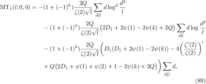
Abstract
We investigate the exact formula for the second moment of central  -values associated to primitive cusp forms of level one and weight
  ,
,  , which was proved by Kuznetsov in 1994. Nondiagonal terms in this formula are expressed in terms of several convolution sums of divisor functions. We investigate the main terms of the convolution sums and show that they cancel out.
Bibliography: 8 titles.
Export citation and abstract BibTeX RIS
| This research was carried out at Pacific National University and supported by the Russian Science Foundation under grant no. 18-41-05001. |
§ 1. Introduction
Let  be the normalized Hecke basis of the space of holomorphic cusp forms of level one and weight
  . For every function
  we can use the Fourier expansion

in order to define the associated -function
It is possible to construct an analytic continuation of  to the whole complex plane. The so-called completed -function

satisfies the functional equation

One of the central problems in the theory of -functions is to determine the proportion of nonvanishing central -values. Note that the functional equation (4) implies that  for all odd
  . Therefore, it is interesting to consider only even .
Nonvanishing results for central values of -functions are not only of theoretical interest but also have important applications (see [1] for references). One of the most interesting examples of such applications (discovered by Iwaniec and Sarnak [5]) is the nonexistence of Landau-Siegel zeros for Dirichlet -functions of real primitive characters.
The most common approach to nonvanishing problems is the method of moments. In particular, the given technique was used in [1] to prove that  of the -functions associated to holomorphic cusp forms of weight and level one have nonzero central values. The proof is based on the following exact formula for the twisted second moment, which was first obtained by Kuznetsov (preprint 1994, see also [1], Theorem 4.2 for the proof) and independently proved by Iwaniec and Sarnak (see [5], Theorem 17).


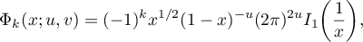
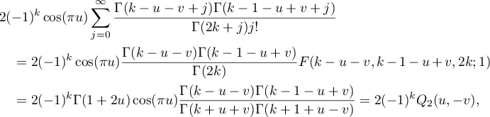
Each summand  can be expressed in terms of hypergeometric functions:
and
where

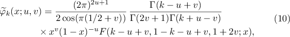
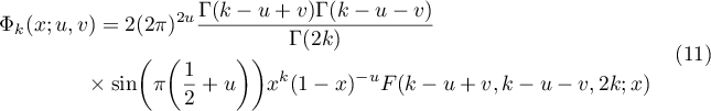
and
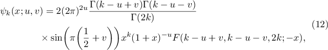
 is the Gamma function,
  is the Gauss hypergeometric function ( definitions and properties of these functions can be found in [7], Chs. 5 and 15) and
where 
For simplicity, let  and
and  . Using the asymptotic expansions for
  and
and  obtained in [1], §5, and then estimating the absolute values of everything in the error terms
  , the following formula was proved in [1], Theorem 6.4:

This is nontrivial for  . We observe that taking an additional smooth average over weight
  , it is possible to obtain a nontrivial asymptotic formula for
  (see [1], Theorem 7.4, for details). Iwaniec and Sarnak [5] showed that a possible approach to demonstrate the nonexistence of Landau-Siegel zeros is to prove an asymptotic formula for the averaged twisted moment for
  . In this sense,
  is a natural barrier caused by the behaviour of the corresponding special functions. Indeed, if
  , then according to [1], Lemma 6.2, we have

and thus the term  is negligibly small. For
  this term is no longer negligible. This is because for large
  the function
  decays exponentially, but for very close to 1 it does not (see [1], §5.3)! As a result, for the left-hand side of (15) will not be negligible. Since does not have oscillatory behaviour, even averaging over will not make smaller. We show below that
So it is reasonable to conjecture that there is a second main term in (14) for . The problem is that this second main term is larger than the main term in (14). It might seem that this strange phenomenon makes it impossible to improve the  nonvanishing result due to Iwaniec and Sarnak, since, as it is shown in [3], the first moment does not change its behaviour for
  (note that when proving results on nonvanishing the twist in the second moment should grow as the square of the twist in the first moment). However, it is widely believed that the percentage of nonvanishing should be
  , and therefore it is reasonable to investigate the second main terms further.
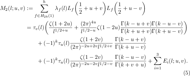
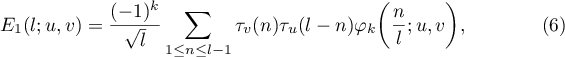
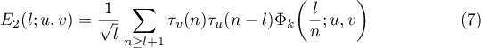
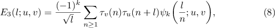
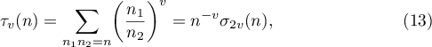
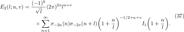
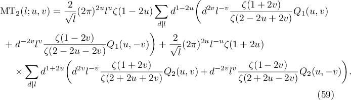
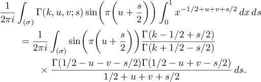
According to (5), there are three convolution sums (6)–(8). Each of them has the following form of a binary additive divisor problem:
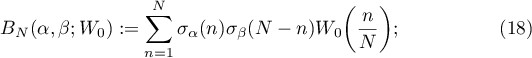
see [6], pp. 531 and 533. This problem has a long history and is very well studied (for references see [2]). An exact formula with a precise form of both the main term and the error term was discovered by Kuznetsov. In this paper we are interested only in the shape of the main terms. In the notation of [6], (4.9) and (4.29), we have

where  and
and  are error terms and

and

where
and
We conjecture that one can apply this result to each . For  let
let

where  is the main term.
Conjecture 1.2. The main term  of the summand
  can be evaluated using (21). For
  the main term of can be evaluated using (20).
Assuming that this conjecture holds, it is possible to evaluate the predicted main term of each . Using the results of [6], it is also possible to evaluate the error terms, but we have not been successful in obtaining any reasonably good estimates for them. This is because the application of the results of [6] unfortunately leads to a dead loop by which we recover back the initial value of the second moment.
The main result of this paper is the following.
Theorem 1.3. Assuming Conjecture 1.2 we have

This theorem asserts that for large  there is no second main term in (14).
§ 2. Special functions
For the convenience of the reader we first recall the definitions and some properties of the Gamma function and the Gauss hypergeometric function. These facts, among others, can be found in [7], Chs. 5 and 15, for example.
For  the Gamma function is defined by means of the Euler integral
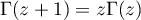
([7], 5.2.1). The Gamma function is a meromorphic function with simple poles at negative integers  . This function satisfies the following functional equations:
([7], 5.5.1) and

([7], 5.5.3). For  one can define the psi-function
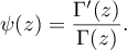
This is a meromorphic function with simple poles at the nonpositive integers . The psi-function satisfies the following functional equation:

(see [7], 5.5.2). For  the Gauss hypergeometric function is defined by the absolutely convergent series
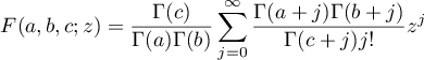
(see [7], 15.2.1). This function can be continued analytically to the whole complex plane. In the case of  and
and  the Gauss hypergeometric function can be evaluated in terms of Gamma functions:

(see [7], 15.4.20).


For  the following identity holds:

Equation (29) follows from [7], 5.12.3. To prove (30) we apply [7], 5.12.1.


and

where  and
and

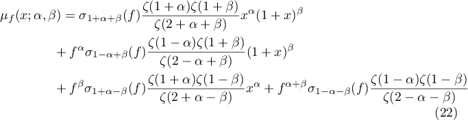
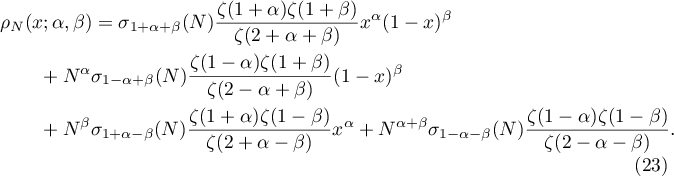
Proof. It follows from [1], (4.15), that

where
In the same way, we obtain

Using [4], Lemma 5.7, to transform the right-hand sides of (35) and (36), we show that

and
where  is defined in [4], §5, and coincides with (33). The lemma is proved.
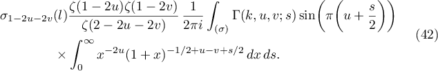
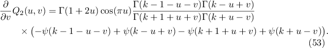
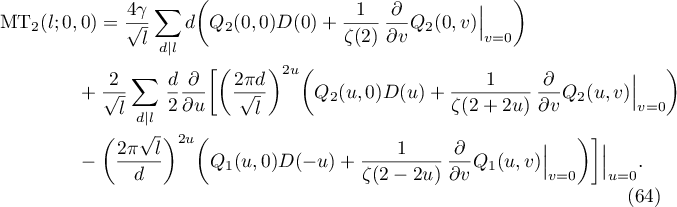
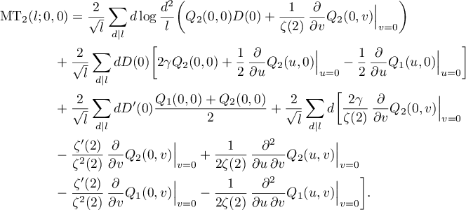
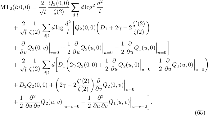
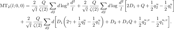
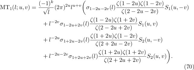
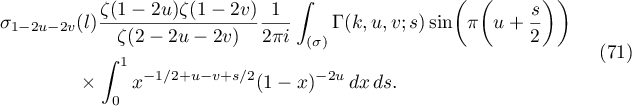
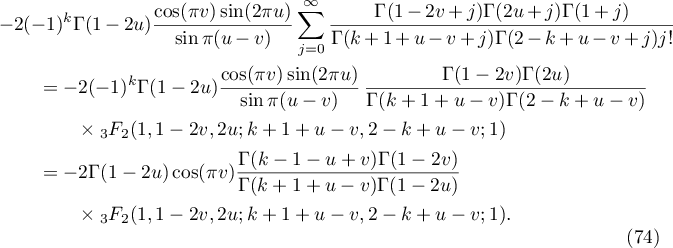
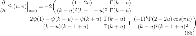
§ 3. Evaluating the main term of 
Replacing the function  in (7) by (32) and using (13) we obtain
Assuming Conjecture 1.2, the main term  of (37) is given by
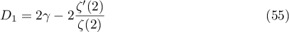
(see (17), (19) and (20)). Let

and

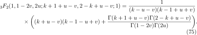
Lemma 3.1. The following identity holds:
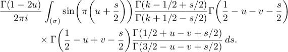
Proof. To prove the lemma we substitute (33) and (22) into (38). In doing so we obtain four similar terms: each of them can be evaluated in the same way. We consider the first and second terms. The first term is given by
To evaluate the integral with respect to we apply (29), getting
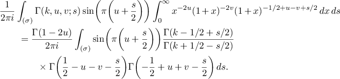
Moving the line of integration to the left and evaluating the residues at 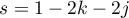 for
for  , we infer
where (28) was used to evaluate the hypergeometric function. Substituting (43) into (42), we obtain the first term in (41).
Let us briefly describe how the second term in (41) can be obtained. In this case, we need to compute

To evaluate the integral with respect to we apply (29). Consequently,

Moving the line of integration to the left and evaluating the residues at for , we show that
where (28) was used to compute the hypergeometric function. The lemma is proved.
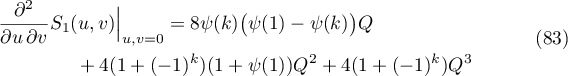
Our next goal is to evaluate  using (41). To this end, we need to study the properties of
  and
and  .
.


and

Proof. It follows from (39) that

and

Thus (46) and a part of (45) are proved. Computing the derivative of (50) with respect to  , we prove (48).
Formula

follows immediately from (40). Since  (see (27)), we prove (47).
Also as a consequence of (40) we have
Letting  on the right-hand side of (53), we show that

Since 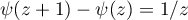 (see (27)), we complete the proof of (45). Letting
  in (53) and then computing the derivative of (53) with respect to , we obtain
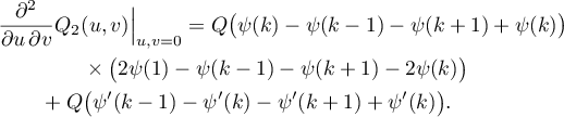
Since  , we finally prove (49). The lemma is proved.
Let

and
Then

Now we are ready to evaluate using (41).
Theorem 3.3. The following formula holds:
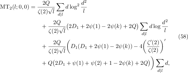
where 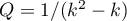 and
and  is defined in (55).
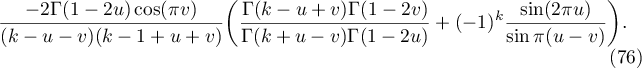
Proof. First, we continue (41) analytically to a region containing . To do this, we rewrite (41) in the following form
The next step is to evaluate the limits of two brackets in (59) as  To this end, we use the Laurent expansion of the Riemann zeta-function

(see [7], 25.2.4). We compute the limit of the first bracket in (59). Using (60), we obtain that it is equal to
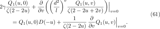
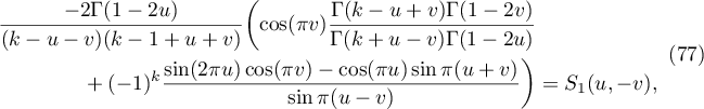
Using (59) and (61), we show that
We need to verify that the right-hand side of (62) is holomorphic at  . For this goal, it is enough to check that
which follows from (44) and (45). Applying L'Hôpital's rule and (60), we compute the limit of the right-hand side of (62) at :
Evaluating the derivative, using (63) and making some transformations, we obtain
Substituting (57) and using (44) and (45), we conclude that
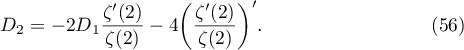
Substituting (55), (56) and (46)–(49), we finally prove (58). Theorem 3.3 is proved.
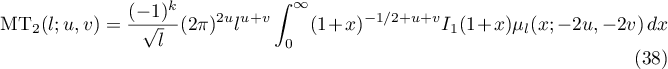
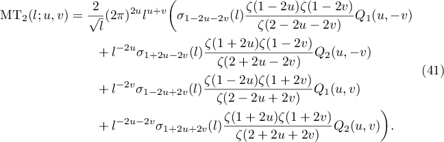
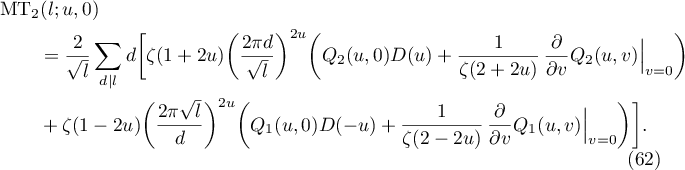
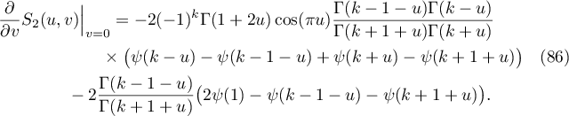
§ 4. Evaluating the main term of

Substituting (31) into (6) and using (13), we have
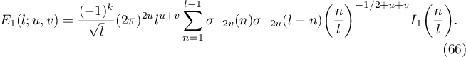
Assuming Conjecture 1.2, the main term of (66) is given by

(see (18), (19) and (21)). Let
and
Lemma 4.1. The following identity holds
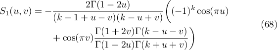
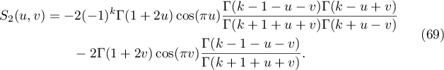
Proof. The proof is similar to that of Lemma 3.1. We substitute (33) and (23) into (67). In this way we obtain four terms that can be evaluated in the same way. We consider the first and fourth terms. The first term is given by
To evaluate the integral with respect to we apply (30). In doing so, we obtain
Moving the line of integration to the left and evaluating the residues at ,  for , we show that
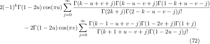
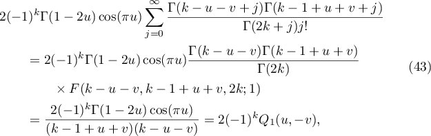
Consider the first sum in (72). Applying (26) twice, we prove that it is equal to
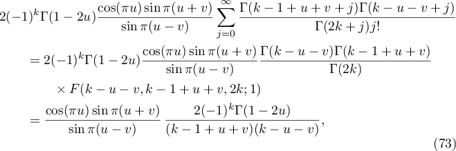
where we have used (28) to evaluate the hypergeometric function.
Consider the second sum in (72). Applying (26) twice, we show that it is equal to
Applying [8], §7.4.4, formula 27 (for  ), we obtain
Substituting (75) into (74) and using (26) twice, we prove that the second sum in (72) is equal to
Summing (73) and (76), we conclude that the integral in (71) is equal to
and therefore we recover the first summand in (70).
Let us briefly describe how we can obtain the fourth term in (70). In this case, we must compute
Moving the line of integration to the left and evaluating the residues at for and  , we have
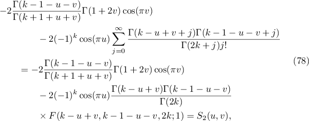
where we have applied (28) to evaluate the hypergeometric function. Lemma 4.1 is proved.
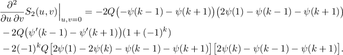
Next, we compute  using (70). For this goal, we study the properties of
  and
and  .
.
Lemma 4.2. The following identities hold:


and
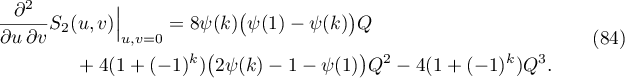
Proof. Equality (79) is a direct consequence of (68) and (69). Furthermore, it follows from (68) and (69) that
and
Substituting in (85) and (86) we obtain (80) by applying the relation

which follows from (27), in the case of (86).
Applying (87), the proof of (81) and (82) follows directly from (68) and (69), respectively. Moreover, we prove (83) by computing the derivative of (85). To show that (84) holds, we compute the derivative of (86) and obtain
Using (87) and the relation

we finally prove (84). The lemma is proved.
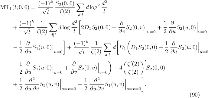
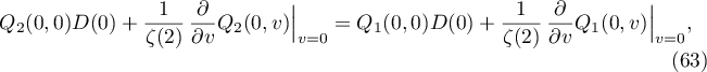
where and is defined in (55).
Proof. Identity (89) is a consequence of (70). More precisely, we proceed similarly to the proof of Theorem 3.3 by starting from (41) and repeating all the steps required to derive (58). Note that in order to prove analytic continuation to the point in Theorem 3.3 we require that (63) holds. Now we need the analogue of this equation:

which is a consequence of (79) and (80). Finally, applying (56), we derive the analogue of (65):