Optimal Interpolation Model for Synthetic Aperture Radar Wind Retrieval

Introduction

Sea surface wind is a crucial parameter for studying the physical quantity of the sea surface and plays an important role in many fields such as weather forecasts (Von Ahn et al., 2006; Friedman et al., 2010), wind energy resource management (Hasager et al., 2011; Chang et al., 2015), wave numerical simulation (Cavaleri et al., 2007; Sullivan and McWilliams, 2010), and oil spill monitoring (Espedal, 1999; Cheng et al., 2014). Because of the limited spatial and temporal coverage, high-precision sea surface wind data acquired from buoys, ships and offshore platforms cannot meet the growing demand (Zhou et al., 2017).

In recent decades, with the development of satellite remote sensing, the technology of acquiring sea surface wind data using satellite sensor detection data has gradually matured and improved. Among various satellite sensors, microwave radiometers and scatterometers play an important role in providing global sea surface wind data. However, microwave radiometers and scatterometers can acquire only low-spatial resolution (12.5–50 km) sea surface wind data. This relatively low spatial resolution is best suited for open-ocean studies and limits our ability to study the marine atmospheric boundary layer and ocean processes in coastal regions (Duan et al., 2017; Fang et al., 2018). However, spaceborne synthetic aperture radar (SAR) can alleviate this problem because it has all-weather day and night observation capabilities, and it can retrieve sea surface wind with a spatial resolution for nearly two orders of magnitude higher (subkilometer) than that of microwave radiometers and scatterometers (Monaldo et al., 2001). It has a unique advantage for studies in coastal region.

For angles of incidence between 15° and 70°, the copolarization radar backscatter from the sea surface received by the satellite sensor is mainly caused by small-scale sea surface roughness, which is strongly influenced by sea surface wind. This backscatter makes it possible to extract sea surface wind from SAR images. In 1979, Weissman et al. (1979) noted that there is a correlation between the intensity of SAR images and the sea surface wind field. The wind streak direction in the images is nearly aligned with the wind direction, and the SAR normalized radar cross section (NRCS) is related to the wind vector. Based on this theory, a classic method for sea surface wind retrieval based on wind streaks was developed that retrieves the wind direction and wind speed separately. Inversion methods for the wind direction (which has an ambiguity of 180°) mainly include the Fourier transform (Gerling, 1986; Lehner et al., 1998), the wavelet transform (Fichaux and Ranchin, 2002; Leite et al., 2010), and local gradient analysis (Sobel operator, numerical differentiation) (Jiang et al., 2011a; Jiang et al., 2011b; Rana et al., 2016; Zhou et al., 2017); the 180° ambiguity can be removed by referencing numerical weather prediction model wind, Doppler shifts or land shadows (Horstmann and Koch, 2003; Christiansen and Jochen, 2006; Mouche et al., 2012), and the wind speed is acquired by the geophysical model function (GMF) based on the wind direction. Due to the specific meteorological conditions required for wind streaks, relevant studies have shown that only 35%–48% of SAR images have wind streak features (Levy, 2001; Zhao et al., 2016; Rana et al., 2019). Moreover, other ocean phenomena also have features similar to wind streak, such as ocean internal waves and surface currents, which makes it more difficult to automatically acquire sea surface wind information from streak features. When the wind direction cannot be acquired or if the error is large, the wind speed acquisition and accuracy will be directly affected. A wind direction error of 30° introduces wind speed uncertainty up to 40% (Lehner et al., 1998; Horstmann et al., 2000), which makes the inversion method based on wind streaks somewhat limited in application. Therefore, some researchers have explored the methods of retrieving wind speed directly without wind direction input, such as Komarov model (Komarov et al., 2014; La et al., 2017) and electromagnetic model (La et al., 2018).

In 2002, Portabella et al. (2002) proposed a sea surface wind inversion method based on the Bayesian theory, which consists of estimating the wind from an SAR NRCS measurement, a GMF model, a prior wind from the numerical prediction model, and their associated uncertainties. This approach constructs a variational formulation, in which the optimum wind vector is determined by minimizing a cost function. The effectiveness of the proposed method is proven with European Remote Sensing Satellite-2 (ERS-2), Envisat, RADARSAT-1, and Gaofen-3 (GF-3) SAR sea surface wind retrieval applications (Portabella et al., 2002; Adamo et al., 2014; Wang et al., 2017). The variational model inversion (VAR) method does not need to consider wind streak information and can simultaneously acquire the wind direction and wind speed. It can be an excellent complement to the wind retrieval method based on wind streaks. However, since the variational formulation is a nonlinear equation, the analytical solution of the formulation cannot be acquired. Only the optimum solution can be acquired by the iterative or enumeration method, so the solution is unstable and the time latency is long (Choisnard and Laroche, 2008; Jiang et al., 2017).

In this article, we propose a new wind retrieval method by applying the optimal interpolation (OI) theory to construct a formula, which combined the SAR information with background information from the numerical prediction model, assuming that all sources of information contain errors and are well-characterized. The retrieval wind vector can be quickly acquired through the derivation of the OI formula.

The remaining sections are organized as follows. In Geophysical Model Function, different GMFs are introduced. In Variational Model Inversion Formulation for Wind Retrieval, the VAR sea surface wind retrieval method and its solutions are introduced. In Optimal Interpolation Model for Wind Retrieval, we present the OI model and its solution in detail. Simulation experiments on the wind retrieval accuracy and time latency are discussed in Simulation Experiments and Discussion. Applications of the Sentinel-1 SAR wind retrieval are shown in Application to Sentinel-1 Synthetic Aperture Radar Data and Discussion. Finally, conclusions are given in Conclusions.

Geophysical Model Function

The GMF is an empirical function established by many statistical experiments to describe the relationship between the NRCS and sea surface wind. The C-band model (CMOD) GMF was first developed for scatterometer on the ERS satellite operating at the C-band and vertical transmitting/vertical receiving (VV) (E.P.W. and Attema, 1986). In 1993, CMOD4 was obtained by fitting the scatterometer NRCS and the European Center for Medium-Range Weather Forecasts (ECMWF) analysis wind field (Stoffelen and Anderson, 1997), but CMOD4 resulted in certain errors at high wind speeds, so CMOD_IFR2, CMOD5, and CMOD5. N were proposed (Quilfen et al., 1998; Hersbach et al., 2007; Hersbach, 2010). CMOD is formulated as follows:

In Eq. 1, ${\sigma }^o$ is the SAR NRCS, $V$ is the wind speed at a height of 10 m above the sea surface, $\theta$ is the SAR incidence angle, and $\varphi$ is the relative wind direction measured with respect to the horizontal radar look direction. $B_0$, $B_1$, and $B_2$describe the main relationship between the wind speed and the incidence angle. $\alpha$ is a power value that depends on the GMF used.

Figure 1 presents the behavior of the four CMOD GMFs as a function of wind direction and wind speed at a given satellite incidence angle of 30° and look direction of 0°. The main difference between the four GMFs is the NRCSs observed for the high wind (greater than 20 m/s) and low wind (less than 2 m/s) (Figure 1A). The NRCS-observed tendencies of wind direction are very similar, but the amplitudes are slightly different (Figure 1B).

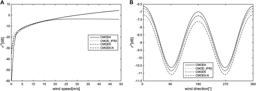
FIGURE 1. Comparison of the CMOD4, CMOD_IFR2, CMOD5, and CMOD5. N NRCS simulations as a function of (A) wind speed (wind direction of 0°) and (B) wind direction (wind speed of 12 m/s).

Variational Model Inversion Formulation for Wind Retrieval

Introduction of the Variational Model Inversion Model for Wind Retrieval

The VAR method proposed by Portabella et al. (2002) based on the Bayesian theory is the most widely used and mature algorithm in addition to SAR image analysis algorithms for wind retrieval. Many scholars have carried out in-depth analyses and application tests (Cameron et al., 2007; Jiang et al., 2011a; Jiang et al., 2011b; Jiang et al., 2014). It is assumed that the SAR observation and the background information error follow a Gaussian distribution and are uncorrelated. In the variational framework, the analysis wind is obtained through the minimization of a cost function, which can be expressed as follows:

where $J_o$ is the observation term and $J_b$ is the background term. For a single SAR NRCS observation, $J_o$ is derived from and expressed as the following form:

The physical meanings of the symbols in Eq. 3 are shown in Table 1.

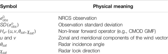
TABLE 1. The physical meanings of the symbols in Eq. 3.

$J_b$ is expressed as the following form:

where $u_b$ and $v_b$ are the zonal and meridional components of the background wind vector, respectively, and they are independent and have equal standard deviations of their error [i.e. $SD\left(u_b\right)=SD\left(v_b\right)$].

There are three tested methods to acquire the optimum wind vector by minimizing Eq. 2: enumeration VAR (EnVAR), Monte Carlo VAR (MCVAR), and damped Newton VAR (DNVAR).

Enumeration Variational Model Inversion

Portabella et al. (2002) proposed the EnVAR solution of the variational model. First, a wide range of winds (e.g., $u\in [-20\text{m/s},20\text{m/s}]$ and $v\in [-20\text{m/s},20\text{m/s}]$ with a step size of 0.25 m/s) around the background wind vector are used as “trial” winds. Then, equation (2) is used to calculate the $J$ values corresponding to the “trial” winds. The “trial” wind vector value that corresponds to a minimum $J$ is the optimum wind vector.

Monte Carlo Variational Model Inversion

Choisnard and Laroche (2008) proposed the MCVAR solution of the variational model. First, the “trial” winds are simulated by adding a random Gaussian error to the observation and background values. Then, Eq. 2 is used to calculate the $J$ values corresponding to the “trial” winds. The “trial” wind vector value that corresponds to a minimum $J$ is the optimum wind vector.

Damped Newton Variational Model Inversion

Jiang et al. (2017) proposed the DNVAR solution of the variational model. They introduced a damped Newton method to form the iteration function of the optimum wind vector. By calculating the second-order derivative of $J$, the iteration direction and step can be determined, and then, the optimum wind vector can be obtained through iteration.

EnVAR, MCVAR, and DNVAR require many iterations to calculate the optimum solution. The wind retrieval accuracy and time latency of the three methods were tested by Jiang et al. (2017) on simulated data and Envisat/advanced synthetic aperture radar (ASAR) data. The experimental results show that the retrieval accuracies of the three methods are slightly different, and all of the errors are smaller than the background wind errors. The computational complexity of DNVAR is lower than that of EnVAR and MCVAR.

Optimal Interpolation Model for Wind Retrieval

The OI equation was first derived by Eliassen in 1954. Gandi independently introduced the multivariate OI equation in 1963 and applied it to the objective analysis of meteorological data in the Soviet Union. Gandi’s work had a profound impact on meteorological research and operational applications. The OI scheme has become a multistatistical data assimilation operational analysis program (Bengtsson et al., 1981; Kalnay, 2003). Based on the OI theory, this study constructs an OI formulation that can be applied to the SAR sea surface wind inversion.

Assume that SAR observations $y$ can be expressed as:

where $H$ is the nonlinear forward operator, $x={(u,v)}^{\text{T}}$ is the real wind vector, and ${\epsilon }_o$ is the observation error. Given the background wind vector $x_b={(u_b,v_b)}^{\text{T}}$, the analysis wind vector $x_a$ can be obtained according to the OI theory, which can be expressed as follows:

where $K$ is the weight matrix.

The analysis wind vector errors ${\epsilon }_a$ and background wind vector errors ${\epsilon }_b$ can be defined as follows:

Substituting Eq. 6 into Eq. 7 yields

Then, we perform a linearization of the nonlinear observation operator around the background state, implicitly assuming that the truth is not too far from the background. Taylor expansion of $H\left(x\right)$ at the value of background wind vector $x_b$ is

where $H^{\text{'}}\left(x_b\right)=(\frac{\partial H}{\partial u}{|}_b,\frac{\partial H}{\partial v}{|}_b)$, assuming ${\rm H}=H^{\text{'}}\left(x_b\right)$. Substituting Eq. 10 into Eq. 9, we have

Now, we transform the problem of the optimal analysis wind vector into the problem of minimizing the mean square error of the analysis wind vector. The minimum mean square error of the analysis wind vector can be expressed as the following form:

It is difficult to obtain the solution of Eq. 12, so the problem is converted into the problem of minimizing the trace of the analysis wind vector error covariance matrix, which can be expressed as follows:

To form the analysis wind vector error covariance, we multiply Eq. 11 by its transpose:

Assuming that the background wind vector and the observed wind vector are both unbiased, then $E\left({\epsilon }_b\right)=0,E\left({\epsilon }_o\right)=0$, and the observation errors are a scalar for a single NRCS observation, Thus, $E\left({\epsilon }_o{\epsilon }_o^{\text{T}}\right)={\epsilon }_o^{\text{2}}$ and $E\left({\epsilon }_b{\epsilon }_o^{\text{T}}\right)=E\left({\epsilon }_o{\epsilon }_b^{\text{T}}\right)=0$. Assuming a background wind vector error covariance matrix $B=E\left({\epsilon }_b{\epsilon }_b^{\text{T}}\right)$, we have

We now minimize the mean square error of the analysis wind vector with respect to the weight matrix $K$. Thus,

Substituting Eq. 15 into Eq. 16 yields

Solving for $K$ yields

Then, we have the expression of the analysis wind vector:

Therefore, given the background wind vector error covariance $B$ and the observation error ${\epsilon }_o$, only the differential result of the forward operator $H$ at the background wind vector $x_b$ needs to be calculated, and the analytical solution of the analysis wind vector can be obtained by using Eq. (19).

Simulation Experiments and Discussion

In the following simulation experiments, we consider a satellite configuration with incidence angle ${\theta }_{sat}{=30}^{\mathrm{°}}$ and radar look direction ${\chi }_{sat}=\text{0}$; the observation error of the NRCS measurement is 10%, and the standard deviation error for the background wind components is 1.7 m/s (Portabella et al., 2002). Because CMOD5 and CMOD5.N take into account NRCS saturation at high winds and CMOD5 is more widely used in SAR wind retrieval, we choose the CMOD5 GMF as nonlinear forward operator.

OI wind retrieval is evaluated using Eq. 19. The result is compared to the direct wind retrieval (hereafter called DIRECT), in which a fixed a priori wind direction (from the background wind vector) is directly inserted into the CMOD5 GMF, and VAR wind retrieval is evaluated using DNVAR.

Optimal Interpolation Wind Retrieval Accuracy Analysis

Case with Varying Background Wind Errors

In this section, we consider the case in which the background wind vector contains regular errors in both the wind direction and the wind speed. Assuming true wind speeds $V_T$ of 5, 12, and 25 m/s which are adopted as low-, moderate-, and high wind speed cases respectively, and true wind directions ${\varphi }_T$ of 0° and 45°, given the background wind direction error ${\varphi }_{BE}\in [-{20}^{\mathrm{°}},{20}^{\mathrm{°}}]$ with a step size of 1° and the background wind speed error $V_{BE}\in [-2\text{m/s},2\text{m/s}]$ with a step size of 0.1 m/s, the OI wind retrieval results are shown in Figures 2–4.

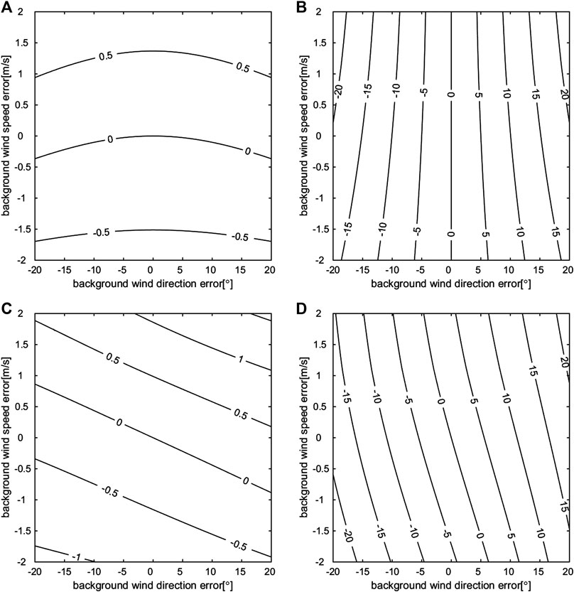
FIGURE 2. Optimal interpolation (OI)-retrieved wind speed errors (A, C) and wind direction errors (B, D) (the isolines) when the true speed is 5 m/s, and the true wind direction is either 0° (A, B) or 45° (C, D); the background wind speed errors (Y axis) and the background wind direction errors (X axis) are given.

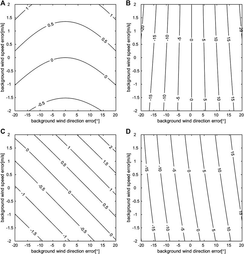
FIGURE 3. OI-retrieved wind speed errors (A, C) and wind direction errors (B, D) (the isolines) when the true speed is 12 m/s, and the true wind direction is either 0° (A, B) or 45° (C, D); the background wind speed errors (Y axis) and the background wind direction errors (X axis) are given.

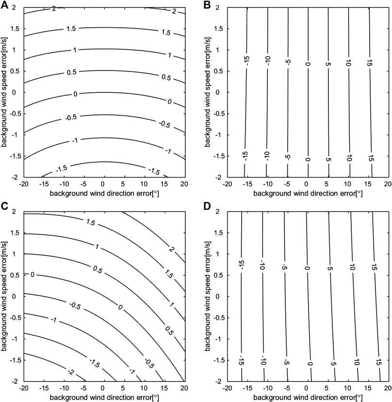
FIGURE 4. OI-retrieved wind speed errors (A, C) and wind direction errors (B, D) (the isolines) when the true speed is 25 m/s, and the true wind direction is either 0° (A, B) or 45° (C, D); the background wind speed errors (Y axis) and the background wind direction errors (X axis) are given.

The retrieval results, which assume that $V_T=5\text{m/s}$, are shown in Figure 2. When ${\varphi }_T{=\text{0}}^{\mathrm{°}}$, the OI wind speed error $V_{OE}$ increases with $V_{BE}$ but is smaller than $V_{BE}$ by approximately 50% (Figure 2A). The OI wind direction error ${\varphi }_{OE}$ increases with ${\varphi }_{BE}$ and is slightly smaller than ${\varphi }_{BE}$ overall. In some cases, ${\varphi }_{OE}$ is greater than 20° (Figure 2B). When ${\varphi }_T{=45}^{\mathrm{°}}$ (Figures 2C,D), $V_{OE}$ increases slightly, and ${\varphi }_{OE}$ is slightly changed compared with ${\varphi }_T{=\text{0}}^{\mathrm{°}}$, but the symmetrical distribution structure with $V_{BE}=0$ and ${\varphi }_{BE}=0$ when ${\varphi }_T{=\text{0}}^{\mathrm{°}}$ is changed.

The retrieval results, which assuming $V_T=12\text{m/s}$, are shown in Figure 3. The retrieved wind vector errors are generally similar to $V_T=5\text{m/s}$. Compared with $V_T=5\text{m/s}$, $V_{OE}$ increases slightly; most $V_{OE}$ values are smaller than 2 m/s, and the maximum $V_{OE}$ is greater than 2 m/s when ${\varphi }_T{=45}^{\mathrm{°}}$ (Figure 3C); ${\varphi }_{OE}$ decreases slightly, and the maximum ${\varphi }_{OE}$ is smaller than 20° when ${\varphi }_T{=45}^{\mathrm{°}}$ (Figure 3D).

The retrieval results, which assuming $V_T=25\text{m/s}$, are shown in Figure 4. Compared with low and moderate true wind speeds, $V_{OE}$ is further increased, and the maximum $V_{OE}$ values are both greater than 2 m/s for different ${\varphi }_T$, but most $V_{OE}$ values are still less than 2 m/s (Figures 4A,C). In contrast, ${\varphi }_{OE}$ is obviously decreasing, and similarly, for different ${\varphi }_T$, the maximum ${\varphi }_{OE}$ is less than 20° (Figures 4B,D).

Overall, $V_{OE}$ increases with $V_{BE}$ but is smaller than $V_{BE}$. In addition, with the increase in the background wind speed, $V_{OE}$ will also increase. When the background wind speed is small, $V_{OE}$ will be far smaller than $V_{BE}$. When the background wind speed increases, $V_{OE}$ gradually increases and approaches $V_{BE}$. ${\varphi }_{OE}$ increases with ${\varphi }_{BE}$ and is slightly smaller than ${\varphi }_{BE}$. In addition, ${\varphi }_{OE}$ decreases as the background wind speed increases. The change in the background wind direction will change the symmetrical distribution structure of $V_{OE}$ and ${\varphi }_{OE}$ when ${\varphi }_T{=\text{0}}^{\mathrm{°}}$, but it will not change the trends of $V_{OE}$ and ${\varphi }_{OE}$.

Case Involving Adding Regular Errors to Different Background Wind

Given $V_T\in [5\text{m/s},28\text{m/s}]$ with a step size of 1 m/s, and ${\varphi }_T\in [{\text{0}}^{\mathrm{°}},{360}^{\mathrm{°}})$ with a step size of 5°, 1,728 simulated observations are obtained from the true wind vector by the CMOD5 GMF. We simulate four different background wind settings by adding $V_{BE}=[-2\text{m/s},2\text{m/s}]$ and ${\varphi }_{BE}=[-{20}^{\mathrm{°}},{20}^{\mathrm{°}}]$ to the true wind speed and direction, respectively.

Figure 5 presents the OI-retrieved wind direction and speed errors as a function of the background wind under four different background wind error conditions. Adding the same error to different background wind situations will result in different retrieved wind vector errors, which show harmonic patterns under all error conditions of the background wind speed and direction. $V_{OE}$ and ${\varphi }_{OE}$ deviation directions are generally consistent with $V_{BE}$ and ${\varphi }_{BE}$ deviation directions (e.g., when $V_{BE}<0$, $V_{OE}<0$ can be obtained, and vice versa). $V_{OE}$ shows an increasing trend as the background wind speed increases (Figures 5A,C,E,G), while ${\varphi }_{OE}$ shows a decreasing trend as the background wind speed increases (Figures 5B,D,F,H).

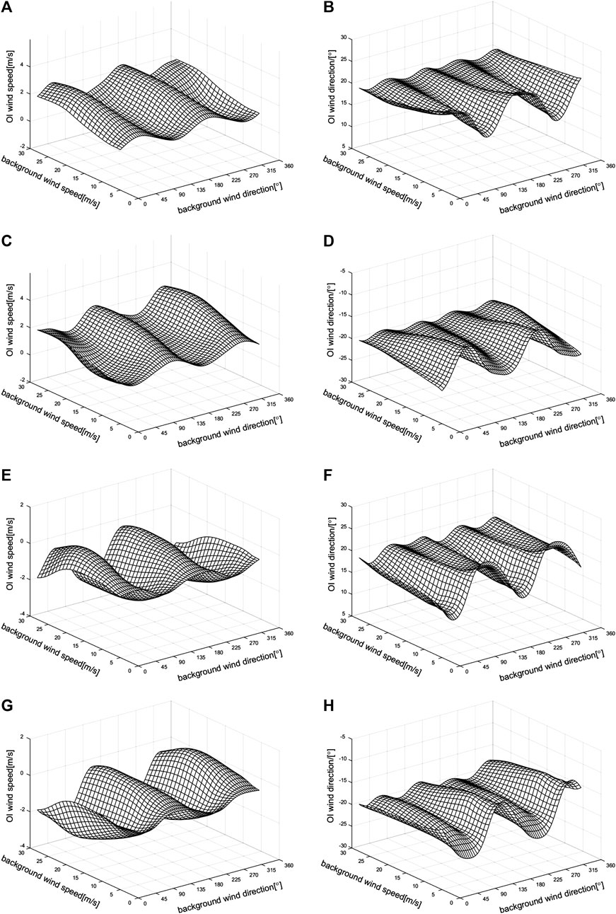
FIGURE 5. OI-retrieved wind errors under different background wind error conditions: for (A) and (B) the background wind speed and direction errors are 2 m/s and 20°, respectively; for (C) and (D), the background wind speed and direction errors are 2 m/s and −20°, respectively; for (E) and (F), the background wind speed and direction errors are −2 m/s and 20°, respectively; for (G) and (H), the background wind speed and direction errors are −2 m/s and −20°, respectively.

Table 2 shows the OI-retrieved wind root mean square error (RMSE), maximum error, and minimum error distributions under different background wind error conditions. The different $V_{BE}$ values will lead to differences in the maximum and minimum errors in the retrieved wind speed and direction. Adding a positive error to the background wind speed (i.e., $V_{BE}=2\text{m/s}$) results in a relatively large maximum of $V_{OE}$ compared to the addition of a negative error, while the maximum of ${\varphi }_{OE}$ is relatively small. The different $V_{BE}$ values do not change the maximum and minimum errors of the retrieved wind, but the error deviation direction will be reversed. The maximum error of the retrieved wind is larger than the background wind error, and the minimum error is smaller than the background wind error. The RMSE of the retrieved wind speed is different under different $V_{BE}$ values. When $V_{BE}=2\text{m/s}$, $V_{OE}$ is relatively large, reaching 1.7 m/s, but is still less than $V_{BE}$. The RMSE of the retrieved wind direction is maintained at 19° under different background wind error conditions, and is smaller than ${\varphi }_{OE}$.

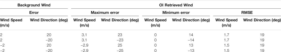
TABLE 2. Comparison of optimal interpolation (OI) retrieved wind speed and direction errors under different error conditions for the background wind speed and direction.

Table 3 lists the ratio of the OI-retrieved wind when the errors are larger than the background wind error under different background wind error conditions. The ratio distribution under different $V_{BE}$ values has the opposite trend. Assuming $V_{BE}=2\text{m/s}$, the retrieved wind ratio is 28.4% when $V_{OE}>2\text{m/s}$, and 20.3% when ${\varphi }_{BE}>{20}^{\mathrm{°}}$. Assuming $V_{BE}=-2\text{m/s}$, the retrieved wind ratio decreases to 24.9% when $V_{OE}>2\text{m/s}$ and increases to 24.8% when ${\varphi }_{BE}>{20}^{\mathrm{°}}$. Overall, under the condition of adding a relatively large error to the background wind speed and direction simultaneously, the ratio of the OI-retrieved wind when its error is larger than the background wind error is less than 30%.

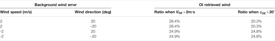
TABLE 3. The ratios of OI-retrieved wind when the error is larger than background wind error.

Case with Varying Incidence Angles

To comprehensively test the performance of the OI method, we adopt incidence angles from 20° to 47°(ESA Communications, 2012) and assume that $V_B\in [5\text{m/s},28\text{m/s}]$ with a step size of 1 m/s, ${\varphi }_B\in [{\text{0}}^{\mathrm{°}},{360}^{\mathrm{°}})$ with a step size of 5°, $V_{BE}=2\text{m/s}$ and ${\varphi }_{BE}={20}^{\mathrm{°}}$. $V_{OE}$ and ${\varphi }_{OE}$ are shown in Figure 6. When the incidence angle is low, the OI-retrieved wind error shows an obvious change trend as the background wind speed increases. $V_{OE}$ increases as the background wind speed increases, and the maximum $V_{OE}$ exceeds 3.5 m/s (Figure 6A); ${\varphi }_{OE}$ decreases as the background wind speed increases, and ${\varphi }_{OE}$ is slightly greater than 20° at low wind speeds (Figure 6B). With the increase in the incident angle, OI-retrieved wind error decreases gradually. When the incident angle is higher than 30°, $V_{OE}$ and ${\varphi }_{OE}$ are less than the background wind error.

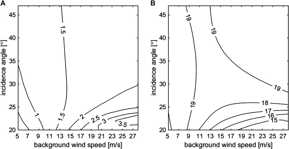
FIGURE 6. OI-retrieved wind speed error (A) and direction error (B) when the incidence angle varies from 20° to 47°. Retrieval accuracy comparison of the OI, variational model inversion (VAR), and DIRECT methods.

Case With Varying Background Wind Errors

In this section, two cases are considered. In one case, the retrieved wind vector errors are analyzed when $V_{BE}=0$ and ${\varphi }_{BE}$contains regular errors. In the other case, the opposite condition is analyzed. Given $V_{BE}\in [-5\text{m/s},5\text{m/s}]$ with a step size of 0.5 m/s, and ${\varphi }_{BE}\in [-{90}^{\mathrm{°}},90^{\mathrm{°}}]$ with a step size of 5°, and assuming true wind speed $V_T$ of 5, 12, and 25 m/s and a true wind direction ${\varphi }_T$ of 45°, the retrieved results of the OI, VAR, and DIRECT are shown in Figures 7, 8.

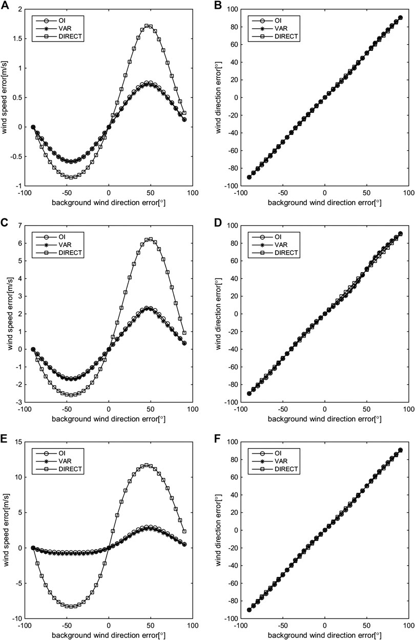
FIGURE 7. Retrieved wind errors of the OI, VAR, and DIRECT methods when the background wind speeds are 5 m/s (A, B), 12 m/s (C, D), and 25 m/s (E, F); the background wind speed contains no errors, and the background wind direction contains regular errors.

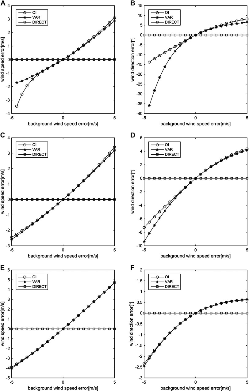
FIGURE 8. Retrieved wind errors of the OI, VAR, and DIRECT methods when the background wind speeds are 5 m/s (A, B), 12 m/s (C, D), and 25 m/s (E, F); the background wind direction contains no errors, and the background wind speed contains regular errors.

When $V_{BE}=0$ and ${\varphi }_{BE}$ contains regular errors (Figure 7), the retrieved wind speed errors of the three wind retrieval methods vary periodically as ${\varphi }_{BE}$ increases. As $V_T$ increases, the retrieved wind speed error of the three wind retrieval methods gradually increases. The $V_{OE}$ and the VAR-retrieved wind speed error $V_{VE}$ are basically the same, and both are smaller than the DIRECT retrieval wind speed error $V_{DE}$. The maximum $V_{OE}$ and $V_{VE}$ are less than 2 m/s, while the maximum $V_{DE}$ is substantially greater than 2 m/s (Figures 7A,C,E). ${\varphi }_{OE}$ and the VAR retrieved wind direction errors ${\varphi }_{VE}$ are basically consistent with ${\varphi }_{BE}$, and both have no obvious improvement with respect to ${\varphi }_{BE}$ (Figures 7B,D,F).

The retrieved results of the OI, VAR, and DIRECT methods when ${\varphi }_{BE}=0$ and $V_{BE}$ contains regular errors are shown in Figure 8. Because the DIRECT-retrieved speed is obtained directly by using the background wind direction, $V_{DE}=0$ when ${\varphi }_{BE}=0$.

Assuming $V_T=5\text{m/s}$ (Figures 8A,B), the OI-retrieved wind agrees with the VAR-retrieved wind when $V_{BE}\in [-2\text{m/s},2\text{m/s}]$ but has a great difference when $V_{BE}<-2\text{m/s}$, where ${\varphi }_{OE}$ is smaller than ${\varphi }_{VE}$ and $V_{OE}$ greater than $V_{VE}$.

Assuming $V_T=12\text{m/s}$ (Figures 8C,D), the difference between the OI- and VAR-retrieved wind is small overall. The OI-retrieved wind accuracy is slightly better than that of VAR when $V_{BE}<\text{0}$ but slightly worse than that of VAR when $V_{BE}\text{>0}$.

Assuming $V_T=25\text{m/s}$ (Figures 8E,F), the OI-retrieved wind agrees with the VAR-retrieved wind. Both wind speed errors are less than $V_{BE}$, and the wind direction errors are less than 2.5°. Compared with $V_T=5\text{m/s}$ and $V_T=12\text{m/s}$, the retrieved wind speed errors increase, and the retrieved wind direction errors decrease.

Overall, both cases show that $V_{OE}$ and ${\varphi }_{OE}$ are smaller than $V_{BE}$ and ${\varphi }_{BE}$. When $V_{BE}=0$ and ${\varphi }_{BE}$ contains regular errors, $V_{OE}$ and $V_{VE}$ are smaller than $V_{DE}$. However, when ${\varphi }_{BE}=0$ and $V_{BE}$ contains regular errors, $V_{DE}$ is the smallest of the three. The retrieved results of the OI and VAR method deviate only slightly.

Case Involving Adding Regular Errors to Different Background Wind

In this section, we use the same simulation data and settings as in Case Involving Adding Regular Errors to Different Background Wind. The RMSEs of the VAR- and DIRECT-retrieved wind are shown in Table 4. Because the DIRECT method uses only the background wind direction information, the retrieved wind speed is greatly affected by ${\varphi }_{BE}$, resulting in a larger RMSE of up to 4 m/s. The VAR-retrieved wind RMSE is less than the background wind error, which is similar to the OI retrieval wind RMSE.

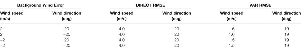
TABLE 4. Comparison of wind errors by different wind retrieval methods.

Time Latency Comparison of the Optimal Interpolation, Variational Model Inversion, and Direct Wind Retrieval Methods

In this section, we use the same simulation data and settings as in Case Involving Adding Regular Errors to Different Background Wind. All the experiments are conducted on the same computer configuration (Intel Core i7-3770 CPU 3.40 GHz, 4 GB RAM). Table 5 shows the time latency comparison of the OI, VAR, and DIRECT wind retrieval methods. In the DIRECT wind retrieval method, the wind speed was obtained based on the enumeration method, that is, the NRCS was first calculated under the given wind direction, wind speed within 0–40 m/s, and intervals of 0.1 m/s, and then the wind speed was obtained by comparison with the input NRCS. Therefore, different settings of the maximum wind speed and the interval will lead to different time latencies, but due to the small amount of calculation, the difference between them is small. Table 5 clearly shows that the time latency of the VAR method is much longer than that of OI and DIRECT methods, and the time latencies of the DIRECT and OI methods are similar.

TABLE 5. Time latency comparison of different wind retrieval methods.

Application to Sentinel-1 Synthetic Aperture Radar Data and Discussion

To evaluate the performance of the OI wind retrieval method on real SAR data, we employ the OI wind retrieval method to retrieve Sentinel-1 SAR sea surface wind. The Sentinel-1 satellites are part of the Global Monitoring for Environment and Security (GMES) programmer implemented by ESA and the European commission. At present, it contains two satellites, namely, Sentinel-1A and Sentinel-1B. The combination of the two satellites shortens the revisiting repetition period from 12 to 6 days. Each Sentinel-1 satellite is equipped with a C-band SAR, which has four independent imaging modes, namely, strip map mode, interferometric wide-swath mode, extra wide-swath mode, and wave mode, and there are four different polarization modes with copolarization (HH and VV) and cross-polarization (HV and VH) (ESA Communications, 2012). This article mainly uses copolarized (VV) data in interferometric wide-swath and extra wide-swath imaging modes, and the corresponding pixel spacing of high-resolution level-1 GRD products is 10 m and 25 m, respectively.

The SAR data used in this study come from the “NOAA high resolution sea surface winds data from synthetic aperture radar (SAR) on the Sentinel-1 satellites” (hereafter called the SARWIND dataset) provided by the National Oceanic and Atmospheric Administration (NOAA) (Monaldo et al., 2016), which processes the Sentinel-1 SAR data by calibration and denoising, and the resolution is reduced to 500 m. This dataset consists of high resolution sea surface wind data produced from the SAR onboard the Sentinel-1A and Sentinel-1B satellites. The high-resolution wind speed (hereafter called the SAR-wind-speed) obtained by the CMOD4 DIRECT method. This dataset utilizes the CoastWatch product format, and the basic archive file is a NetCDF-4 file containing the SAR-wind-speed, SAR NRCS (500 m spatial resolution), numerically predicted wind from the Global Forecast System (GFS, used for the background wind), land mask, and SAR information. The National Data Buoy Center (NDBC) buoy-measured wind data provided by NOAA, which are considered to be the best observation close to the true wind, are used for validation.

In this study, the SARWIND and NDBC buoy data from 2018 were collected, and 2,723 sets of matched data were obtained through spatiotemporal matching and data quality control such as outlier elimination. Because the wind data detected by buoys are usually approximately 5 m away from the sea surface, the wind speed at a height of 10 m was obtained using Eq. 20 (Li and Lehner, 2014).

where $V\left(z_m\right)$ is the wind speed at a height of $z_m$ meters, $V\left(z\right)$ is the wind speed at a height of $z$ meters, and $z_0$ is a constant ($1.52\times {10}^{-4}$).

The results show that the accuracy of the wind direction measured by the buoys is uncertain under low wind speeds (less than 3 m/s) (Freilich, 1997; Liu, 2002; Bentamy et al., 2019). By comparing the matched dataset, the results show that when the buoy-measured wind speed is less than 3 m/s, the RMSE of the background wind direction is 72°, and when the buoy-measured wind speed is greater than 3 m/s, the RMSE of the background wind direction is 35°, with a large difference between the two results. Therefore, to ensure the accuracy of the test, this study excludes all wind speeds less than the 3 m/s.

A comparison of the winds retrieved by the different methods against those measured by the buoys is shown in Figure 9. The RMSE of the OI-retrieved wind speed is 1.4 m/s (Figure 9A), which is lower than that of the background wind speed (1.9 m/s, Figure 9E). The RMSE of the OI-retrieved wind direction is 35° (Figure 9B), which is similar to that of the background wind direction (35°, Figure 9F). These results show that the OI-retrieved wind can effectively improve the background wind, especially in terms of the wind speed. Compared with other wind retrieval methods, the OI-retrieved wind speed accuracy is slightly lower than the VAR-retrieved wind speed accuracy, for which the RMSE of the retrieved wind speed is 1.3 m/s (Figure 9C) but higher than the SAR-wind-speed of 1.7 m/s (Figure 9G) and the DIRECT-retrieved wind speed of 1.5 m/s (Figure 9H). Both the retrieved wind directions from the OI and VAR methods have no obvious improvement over the background wind direction.

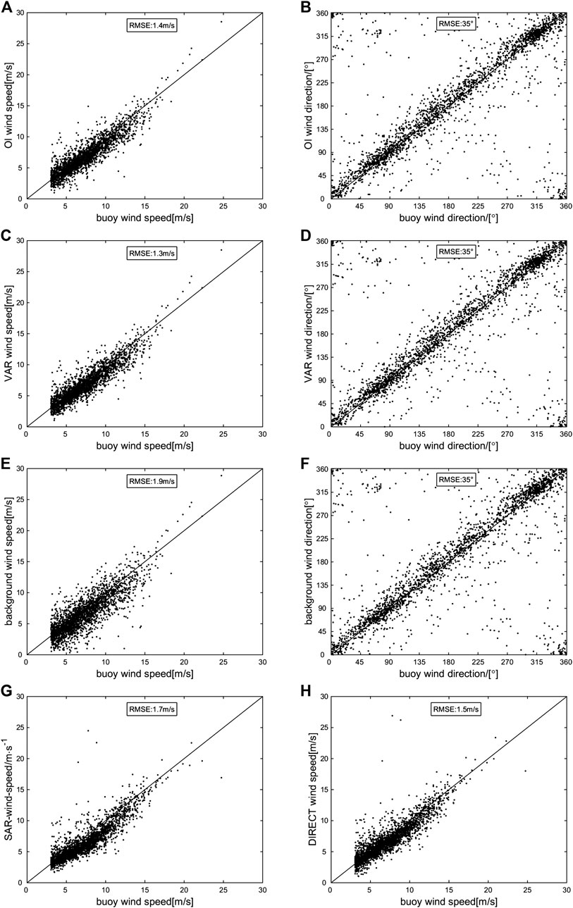
FIGURE 9. Scatter plots of different retrieved winds against the NDBC buoy observations for wind: (A, B) OI-retrieved wind vs. the NDBC buoy observations for wind speed and wind direction, respectively; (C, D) VAR-retrieved wind vs. the NDBC buoy observations for wind speed and wind direction, respectively; (E, F) background wind vs. the NDBC buoy observations for wind speed and wind direction, respectively; (G) synthetic aperture radar-wind-speed vs. NDBC buoy observations for wind speed; (H) CMOD5 retrieved wind speed vs. NDBC buoy observations for wind speed.

The time latency comparison of the OI, VAR, and DIRECT wind retrieval methods on the test dataset is shown in Table 6. The computer configuration is the same as that in Section 5.3. The result is similar to the simulation experiment in which the time latencies of the OI and DIRECT methods are similar, and far lower than that of the VAR method.

TABLE 6. Time latency comparison of different wind retrieval methods.

Conclusions

In this study, we propose a new SAR sea surface wind retrieval method called the OI wind retrieval method. Based on the OI theory and taking errors from all relevant sources into account, the method can acquire wind directions and wind speeds simultaneously. The OI method differs from the VAR wind retrieval method as follows:

1. The OI method is based on the OI theory, which is different from the VAR method, which is based on the Bayesian theory. It does not need to assume that observation errors and background errors follow Gaussian distributions.

2. The OI method can quickly acquire unique optimum wind, while the VAR method needs to find the optimal solution through an optimization algorithm, which is time consuming, and the optimal solutions acquired by different optimization algorithms are different. This is of great significance for the practical application of SAR wind retrieval.

For simulation experiments and practical applications, the accuracy and time latency of the OI method were systematically analyzed and compared with those of the DIRECT and VAR methods. The experimental results are as follows:

1. The OI-retrieved wind error is less than the background wind error; in particular, the accuracy of the OI-retrieved wind speed is significantly improved, so the OI method can be used to retrieve sea surface wind from SAR.

2. The accuracy of the OI-retrieved wind is similar to that of the VAR-retrieved wind but significantly higher than that of the DIRECT-retrieved wind. The time latency of the OI method is the shortest.

The OI method has practical application advantages in SAR wind retrieval and is an alternative to the VAR method. At the same time, it should be noted that both VAR and OI methods need a background wind with good accuracy. When the background wind error is large, the accuracy of retrieved wind will decrease significantly.

Data Availability Statement

The original contributions presented in the study are included in the article/supplementary materials, further inquiries can be directed to the corresponding author/s.

Author Contributions

WZ, wrote the manuscript; HS and JX, contributed the main idea; and ZJ, designed the experiments. All the authors have read and approved the submitted manuscript.

Funding

The research was supported by the National Natural Science Foundation of China (41275113) and the Foundation of State Key Laboratory of Geo-information Engineering (SKLGIE2018-ZZ-8).

Conflict of Interest

The authors declare that the research was conducted in the absence of any commercial or financial relationships that could be construed as a potential conflict of interest.

Acknowledgments

The SAR and GFS data are from the “NOAA high resolution sea surface winds data from synthetic aperture radar (SAR) on the Sentinel-1 satellites ” provided by the National Oceanic and Atmospheric Administration (NOAA) (available online at ftp://ftp.nodc.noaa.gov/pub/data.nodc/sar-winds/sentinel1/2018/). The NDBC buoy data are available at ftp://ftp.nodc.noaa.gov/pub/data.nodc/ndbc/cmanwx/2018/.

References

Adamo, M., Rana, F. M., De Carolis, G., and Guido, P. (2014). Assessing the bayesian inversion technique of C-band synthetic aperture radar data for the retrieval of wind fields in marine coastal areas. J. Appl. Remote Sens. 8 (1), 083531. doi:10.1117/1.jrs.8.083531
Attema, E. P. W. (1986). "An experimental campaign for the determination of the radar signature of the ocean at C-band," in Proceedings of ,Third International Colloquium on Spectral Signatures of Objects in Remote Sensing SP-247, LesArcs, France, 791–799.
Bengtsson, L., Ghil, M., and Källén, E. (1981). Dynamic meteorology: data assimilation methods. New York, NY: Springer,.
Bentamy, A., Mouche, A., Grouazel, A., Moujane, A., and Mohamed, A. A. (2019). Using sentinel-1a sar wind retrievals for enhancing scatterometer and radiometer regional wind analyses. Int. J. Rem. Sens. 40 (3), 1120–1147. doi:10.1080/01431161.2018.1524174
Cameron, I. D., Iain, H., and Walker, N. (2007). "A novel method for estimating offshore wind fields using synthetic aperture radar and meteorological model data," in Paper presented at the 2007 IEEE international geoscience and remote sensing symposium, Barcelona, Spain, July 23-28, 2007 (IEEE).
Cavaleri, L., Alves, J. H. G. M., Ardhuin, F., Babanin, A., Banner, M., Belibassakis, K., et al. (2007). Wave modelling – the state of the art. Prog. Oceanogr. 75 (4), 603–674. doi:10.1016/j.pocean.2007.05.005
Chang, R., Zhu, R., Badger, M., Bay HasagerHasager, C., Xing, X., and Jiang, Y. (2015). Offshore wind resources assessment from multiple satellite data and wrf modeling over south China sea. Rem. Sens. 7 (1), 467–487. doi:10.3390/rs70100467
Cheng, Y., Liu, B., Li, X., Nunziata, F., Xu, Q., Ding, X., et al. (2014). Monitoring of oil spill trajectories with cosmo-skymed X-band sar images and model simulation. IEEE J. Sel. Top. Appl. Earth Observations Remote Sensing. 7 (7), 2895–2901. doi:10.1109/jstars.2014.2341574
Choisnard, J., and Laroche, S. (2008). Properties of variational data assimilation for synthetic aperture radar wind retrieval. J. Geophys. Res. 113, C5. doi:10.1029/2006jc004042
Christiansen, M., Koch, W., Horstmann, J., Hasager, C., and Nielsen, M. (2006). Wind resource assessment from C-band sar. Remote Sens. Environ. 105 (1), 68–81. doi:10.1016/j.rse.2006.06.005.
Duan, B., Zhang, W., Yang, X., Dai, H., and Yi, Y. (2017). Assimilation of typhoon wind field retrieved from scatterometer and sar based on the huber norm quality control. Rem. Sens. 9, 10. doi:10.3390/rs9100987
ESA Communications (2012). Sentinel-1: esa’s radar observatory mission for gmes operational services. Oakville, ON, Canada: ESA Communications.
Espedal, H. A. (1999). Satellite sar oil spill detection using wind history information. Int. J. Rem. Sens. 20 (1), 49–65. doi:10.1080/014311699213596
Fang, H., Xie, T., Perrie, W., Zhang, G., Yang, J., and He, Y. (2018). Comparison of C-band quad-polarization synthetic aperture radar wind retrieval models. Rem. Sens. 10, 9. doi:10.3390/rs10091448
Fichaux, N., and Ranchin, T. (2002). Combined extraction of high spatial resolution wind speed and wind direction from sar images: a new approach using wavelet transform. Can. J. Rem. Sens. 28 (3), 510–516. doi:10.5589/m02-038
Freilich, M. H. (1997). Validation of vector magnitude datasets: effects of random component errors. J. Atmos. Ocean. Technol. 14 (3), 695–703. doi:10.1175/1520-0426(1997)014<0695:vovmde>2.0.co;2
Friedman, K. S., Todd, D., Pichel, W. G., Clementecolón, P., and Hufford, G. (2010). Using spaceborne synthetic aperture radar to improve marine surface analyses. Weather Forecast. 16 (2), 270–276. doi:10.1175/1520-0434(2001)016<0270:USSART>2.0.CO;2.
Gerling, T. W. (1986). Structure of the surface wind field from the seasat sar. J. Geophys. Res. 91 (C2), 2308–2320. doi:10.1029/jc091ic02p02308
Hasager, C. B., Badger, M., Peña, A., Larsén, X. G., and Bingöl, F. (2011). Sar-based wind resource statistics in the baltic sea. Rem. Sens. 3 (1), 117–144. doi:10.3390/rs3010117
Hersbach, H. (2010). Comparison of C-band scatterometer Cmod5.N equivalent neutral winds with ecmwf. J. Atmos. Ocean. Technol. 27, 721–736. doi:10.1175/2009jtecho698.1
Hersbach, H., Stoffelen, A., and de Haan, S. (2007). An improved C‐band scatterometer ocean geophysical model function: cmod5. J. Geophys. Res. 112, C3. doi:10.1029/2006jc003743
Horstmann, J., and Koch, W. (2003). "Ocean wind field retrieval using ENVISAT ASAR data," in IGARSS 2003. 2003 IEEE international geoscience and remote sensing symposium. Proceedings (IEEE Cat. No.03CH37477), Toulouse, France, July, 2003 (IEEE), 3102–3104.
Horstmann, J., Koch, W., Lehner, S., and Tonboe, R. (2000). Wind retrieval over the ocean using synthetic aperture radar with C-band Hh polarization. IEEE Trans. Geosci. Rem. Sens. 38 (5), 2122–2131. doi:10.1109/36.868871
Jiang, Z., Li, Y., Yu, F., Chen, G., and Yu, W. (2017). A damped Newton variational inversion method for sar wind retrieval. J. Geophys. Res. Atmos. 122 (2), 823–845. doi:10.1002/2016jd025178
Jiang, Z.-H., Huang, S.-X., He, R., and Zhou, C.-T. (2011a). Regularization method to retrieve synthetic aperture radar sea surface wind. Acta Phys. Sin. 60 (6), 068401. doi:10.7498/aps.60.068401.
Jiang, Z. H., Huang, S. X., Shi, H. Q., Zhang, W., and Wang, B. (2011b). A new research on sea surface wind direction retrieval of synthetic aperture radar image. Acta Phys. Sin. 60, 10. doi:10.7498/aps.60.108402.
Jiang, Z.-H., Zhou, X.-Z., You, X.-B., Yi, X., and Huang, W.-Q. (2014). Analysis on the variational model of synthetic aperture radar sea surface wind retrieval. Acta Phys. Sin. 63 (14), 148401. doi:10.7498/aps.63.148401.
Kalnay, E. (2003). Atmospheric modeling, data assimilation and predictability. Cambridge, United Kingdom: Cambridge University Press.
Komarov, A. S., Zabeline, V., and Barber, D. G. (2014). Ocean surface wind speed retrieval from C-band sar images without wind direction input. IEEE Trans. Geosci. Rem. Sens. 52 (2), 980–990. doi:10.1109/tgrs.2013.2246171
La, T. V., Khenchaf, A., Comblet, F., and Nahum, C. (2017). Exploitation of C-band sentinel-1 images for high-resolution wind field retrieval in coastal zones (iroise coast, France). IEEE J. Sel. Top. Appl. Earth Obs. Remote Sens. 10 (12), 5458–5471. doi:10.1109/JSTARS.2017.2746349.
La, T. V., Khenchaf, A., Comblet, F., and Nahum, C. (2018). Assessment of wind speed estimation from C-band sentinel-1 images using empirical and electromagnetic models. IEEE Trans. Geosci. Rem. Sens. 56 (7), 4075–4087. doi:10.1109/TGRS.2018.2822876.
Lehner, S., Horstmann, J., Koch, W., and Rosenthal, W. (1998). Mesoscale wind measurements using recalibrated ers sar images. J. Geophys. Res. 103 (C4), 7847–7856. doi:10.1029/97jc02726
Leite, G. C., Ushizima, D. M., Medeiros, F. N. S., and de Lima, G. G. (2010). Wavelet analysis for wind fields estimation. Sensors (Basel) 10 (6), 5994–6016. doi:10.3390/s100605994
Levy, G. (2001). Boundary layer roll statistics from sar. Geophys. Res. Lett. 28 (10), 1993–1995. doi:10.1029/2000gl012667
Li, X.-M., and Lehner, S. (2014). Algorithm for sea surface wind retrieval from terrasar-X and tandem-X data. IEEE Trans. Geosci. Rem. Sens. 52 (5), 2928–2939. doi:10.1109/tgrs.2013.2267780
Liu, W. T. (2002). Progress in scatterometer application. J. Oceanogr. 58 (1), 121–136. doi:10.1023/a:1015832919110
Monaldo, F. M., Jackson, C. R., Li, X., Pichel, W. G., and John Sapper, H. (2016). Noaa high resolution sea surface winds data from synthetic aperture radar (sar) on the sentinel-1 satellites. Washington, D.C: NOAA National Centers for Environmental Information.
Monaldo, F. M., Thompson, D. R., Beal, R. C., Pichel, W. G., and Clemente-Colon, P. (2001). Comparison of sar-derived wind speed with model predictions and ocean buoy measurements." IEEE Trans. Geosci. Rem. Sens. 39 (12), 2587–2600. doi:10.1109/36.974994
Mouche, A. A., Collard, F., Bertrand, C., Dagestad, K.-F., Guitton, G., Johannessen, J. A., et al. (2012). On the use of Doppler shift for sea surface wind retrieval from sar. IEEE Trans. Geosci. Rem. Sens. 50 (7), 2901–2909. doi:10.1109/tgrs.2011.2174998
Portabella, M., Stoffelen, A., and Johannessen, J. A. (2002). Toward an optimal inversion method for synthetic aperture radar wind retrieval. J. Geophys. Res. 107 (C8), 3088. doi:10.1029/2001jc000925
Quilfen, Y., Chapron, B., Elfouhaily, T., Katsaros, K., and Tournadre, J. (1998). Observation of tropical cyclones by high‐resolution scatterometry. J. Geophys. Res. 103 (C4), 7767–7786. doi:10.1029/97jc01911
Rana, F. M., Adamo, M., Guido, P., De Carolis, G., and Morelli, S. (2016). Lg-mod: a modified local gradient (lg) method to retrieve sar sea surface wind directions in marine coastal areas. J. Sensors. 2016, 7. doi:10.1155/2016/9565208.
Rana, F. M., Adamo, M., Lucas, R., and Palma, B. (2019). Sea surface wind retrieval in coastal areas by means of sentinel-1 and numerical weather prediction model data. Remote Sens. Environ. 225, 379–391. doi:10.1016/j.rse.2019.03.019
Stoffelen, A., and Anderson, D. (1997). Scatterometer data interpretation: estimation and validation of the transfer function Cmod4. J. Geophys. Res. 102 (C3), 5767–5780. doi:10.1029/96jc02860
Sullivan, P. P., and McWilliams, J. C. (2010). Dynamics of winds and currents coupled to surface waves. Annu. Rev. Fluid Mech. 42 (1), 19–42. doi:10.1146/annurev-fluid-121108-145541
Von Ahn, J. M., Sienkiewicz, J. M., and Chang, P. S. (2006). Operational impact of quikscat winds at the noaa ocean prediction center. Weather Forecast. 21 (4), 523–539. doi:10.1175/waf934.1
Wang, H., Yang, J., Mouche, A., Shao, W., Zhu, J., Ren, L., and Xie, C. (2017). Gf-3 sar ocean wind retrieval: the first view and preliminary assessment. Rem. Sens. 9 (7), 694. doi:10.3390/rs9070694
Weissman, D. E., King, D. B., and Thompson, T. W. (1979). Relationship between hurricane surface winds and L-band radar backscatter from the sea surface. J. Appl. Meteorol. 18 (8), 1023–1034. doi:10.1175/1520-0450(1979)018<1023:rbhswa>2.0.co;2
Zhao, Y., Li, X.-M., and Sha, J. (2016). sea surface wind streaks in spaceborne synthetic aperture radar imagery. J. Geophys. Res. Oceans. 121 (9), 6731–6741. doi:10.1002/2016jc012040
Keywords: synthetic aperture radar, sea surface wind, optimal interpolation, variational model inversion, C-band model direct wind retrieval
Citation: Zhang W, Jiang Z, Xiang J and Shi H (2020) Optimal Interpolation Model for Synthetic Aperture Radar Wind Retrieval. Front. Earth Sci. 8:552833. doi:10.3389/feart.2020.552833
Received: 20 April 2020; Accepted: 10 September 2020;
Published: 29 October 2020.
Edited by:
Peng Liu, Institute of Remote Sensing and Digital Earth (CAS), ChinaReviewed by:
W. Linwood Jones, University of Central Florida, United StatesAli Khenchaf, UMR6285 Laboratoire des Sciences et Techniques de l’Information, de la Communication et de la Connaissance (LAB-STICC), France
Copyright © 2020 Zhang, Jiang, Xiang and Shi. This is an open-access article distributed under the terms of the Creative Commons Attribution License (CC BY). The use, distribution or reproduction in other forums is permitted, provided the original author(s) and the copyright owner(s) are credited and that the original publication in this journal is cited, in accordance with accepted academic practice. No use, distribution or reproduction is permitted which does not comply with these terms.
*Correspondence: Hanqing Shi, mask10000@126.com